Broadband Dark Matter Axion Detection using a Cylindrical Capacitor

Abstract

Cosmological axions/axion-like particles can compose a significant part of dark matter; however, the uncertainty of their mass is large. Here, we propose to search the axions using a cylindrical capacitor, in which the static electric field converts dark matter axions into an oscillating magnetic field. Using a static electric field could reduce the fluctuations of the signal background compared to using a superconductor solenoid. In addition, due to the odd CPs of the axions, the coupling to the electric field is different. Axion couples to the electric field via a derivative that carries spatial information of incoming dark matter flux while the coupling to the magnetic field depends on the dark matter density. This difference could be helpful in searching the axion field and studies of the integrity of the new theory, especially if the axions are very light, in which case the magnetic field-induced signal is DC-like. In addition, a cylindrical setup shields the electric field to the laboratory and encompasses the axion-induced magnetic field within the capacitor. The induced oscillating magnetic field can then be picked up by a very sensitive magnetometer. Adding a superconductor ring-coil system into the scheme can further boost the sensitivity and maintain the axion dark matter inherent bandwidth. This proposed setup could be capable of wide mass range searches.

I Introduction

Cosmological observations indicate that 23% of the energy density of the Universe is cold dark matter Planck:2015fie . There are many well-motivated cold dark matter candidates, such as the QCD axion and the string theory-originated axion-like particle (ALP). The QCD axion was originally proposed to solve the strong CP problem Peccei:1977hh ; Peccei:1977ur ; Weinberg:1977ma ; Wilczek:1977pj ; vysotsky ; Kim:1979if ; Shifman:1979if ; Zhitnitsky:1980tq ; Dine:1981rt ; Davidson:1981zd but later was also proved to be a very promising dark matter candidate Preskill:1982cy ; Abbott:1982af ; Dine:1982ah ; Sikivie:1982qv ; Ipser:1983mw ; berezhiani1985 . ALPs generally exist in the string theory where the extradimensions are compactified, which creates many different axion species. Both the QCD axions and the ALPs have been extensively studied for their rich astrophysical and cosmological phenomena. Recently, very light ALPs have received increased attention due to their roles in serving as wave-like dark matter, which can explain many puzzles of galactic halo structure formation Hu:2000ke .

The axion field $a$ generally couples to the electromagnetic fields as:

$${\cal L}_{a\gamma\gamma}=-{g_{a\gamma}\over{4}}a{F}{\tilde{F}}=-g_{a\gamma}~{}a\vec{E}\cdot\vec{B},$$ (1)

where the coupling $g_{a\gamma}$ is related to the axion Peccei-Quinn (PQ) symmetry breaking scale $f_{a}$ by $g_{a\gamma}=c_{\gamma}\alpha/(\pi f_{a})$, $\alpha=1/137$ is the fine structure constant, and $c_{\gamma}$ is a model-dependent coefficient of order one. (e.g., $c_{\gamma}=-0.97$ in the KSVZ axion model and 0.36 in the DFSZ axion model.) The axion also couples to electrons, protons, etc., as follows: ${\cal L}_{af}={(g_{f}/f_{a})}\partial_{\mu}a\bar{\psi}_{f}\gamma^{\mu}\gamma^{5}\psi_{f}~{},$ where $g_{f}$ is a model-dependent factor of order one, and $\psi_{f}$ is the respective fermion field. The axion acquires a small mass from the nonperturbative instanton effects. For the QCD axions, the mass $m_{a}$ can be generally written as:

$$m_{a}\approx 0.6\times 10^{-5}{\rm eV}\left({10^{12}~{}\text{GeV}\over f_{a}}\right)~{}.$$ (2)

However, due to the uncertainties of string instantons, the ALPs mass spans several orders of magnitude.

The axion mass $m_{a}$ and the PQ symmetry breaking scale $f_{a}$ are the two most important parameters of the axion searches. They are constrained by cosmological, astrophysical and laboratory considerations. For example, the QCD axion field received energy from the Standard Model sector during the QCD phase transition. If PQ symmetry breaking occurs after inflation, then $f_{a}\sim 10^{12}$GeV and $m_{a}\sim 10^{-5}$eV, which is often called the classical window. If PQ symmetry breaking occurs before inflation, the initial axion field misalignment angle can be anthropic. In this scenario, the isocurvature perturbation of the cosmic microwave background gives additional constraints Hertzberg:2008wr ; Gao:2019tqt and typically leads to $f_{a}\gtrsim 10^{14}$GeV and $m_{a}\lesssim 10^{-7}$eV. Axion dark matter can also be created by the stochastic case Graham:2018jyp ; Guth:2018hsa , where $m_{a}$ ranges from $10^{-12}$eV to $10^{-4}$eV. For string theory-originated dark matter ALPs, the mass range is much larger Svrcek:2006yi ; Visinelli:2018utg . Currently, there are many experiments around the world looking for axions or ALPs Sikivie:1983ip ; Sikivie:1985yu ; DePanfilis:1987dk ; Hagmann:1990tj ; Ehret:2010mh ; Tam:2011kw ; Wouters:2013iya ; Graham:2013gfa ; Budker:2013hfa ; Sikivie:2013laa ; Stadnik:2013raa ; Ayala:2014pea ; Rybka:2014cya ; Sikivie:2014lha ; TheMADMAXWorkingGroup:2016hpc ; Barbieri:2016vwg ; Kahn:2016aff ; Yang:2016zaz ; Brubaker:2016ktl ; Anastassopoulos:2017ftl ; Abel:2017rtm ; Graham:2017ivz ; McAllister:2017lkb ; Akerib:2017uem ; Du:2018uak ; Marsh:2018dlj ; Zhong:2018rsr ; Lawson:2019brd ; Ouellet:2018beu ; Arza:2019nta ; Yang:2019xdz . Noticeable, the mass range $10^{-6}$eV$\sim 10^{-10}$eV is less explored.

Many axion searching experiments are based on the electromagnetic coupling between axions and photons. For axions with a heavier mass, axion haloscopes such as the ADMX are the most capable ones that can reach the QCD axion parameter spaces within current technology. For lighter mass axions, it could be better to consider a quasistatic picture, in which when a strong static magnetic field is present, the axion-sourced current induces a detectable oscillating magnetic field Sikivie:2013laa .

For very light axions, such as in the fuzzy dark matter regime, the induced magnetic field would be DC-like, which could make it harder to distinguish. Interestingly, the odd CP of the axions makes their couplings to the E field behave differently. The electric field couples to the axion field’s derivative; thus, the source terms carry the directional information of the incoming dark matter flux, in addition to the dark matter local density information. Reorientation of the experimental apparatus could be used to distinguish the signals and the backgrounds. This difference is additionally helpful in studying the axion’s fundamental properties, and it serves a test of the integrity of the Beyond the Standard Model theory.

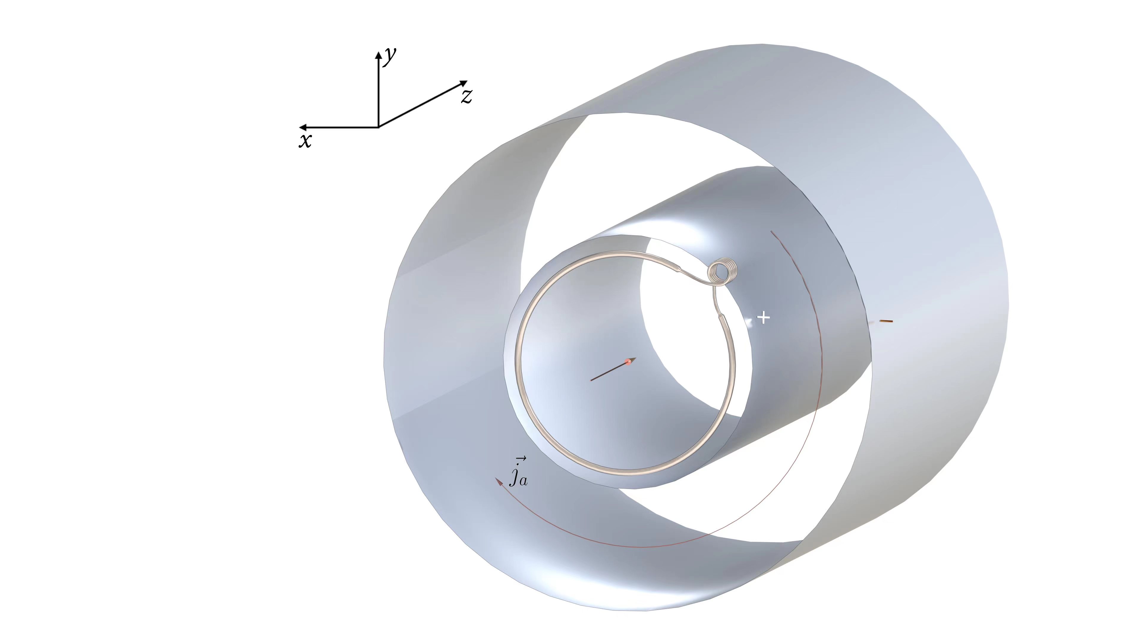
Figure 1: An illustration setup for the proposed experiment. The electric field $\vec{E}$ permeates the region inside the capacitor. The dark matter axions flowing along the $\vec{z}$ axis give rise to an effective electric current density $\vec{j}_{a}$. The effective current density subsequently induces an oscillating magnetic field that can be picked up by a SQUID or other types of magnetometers.

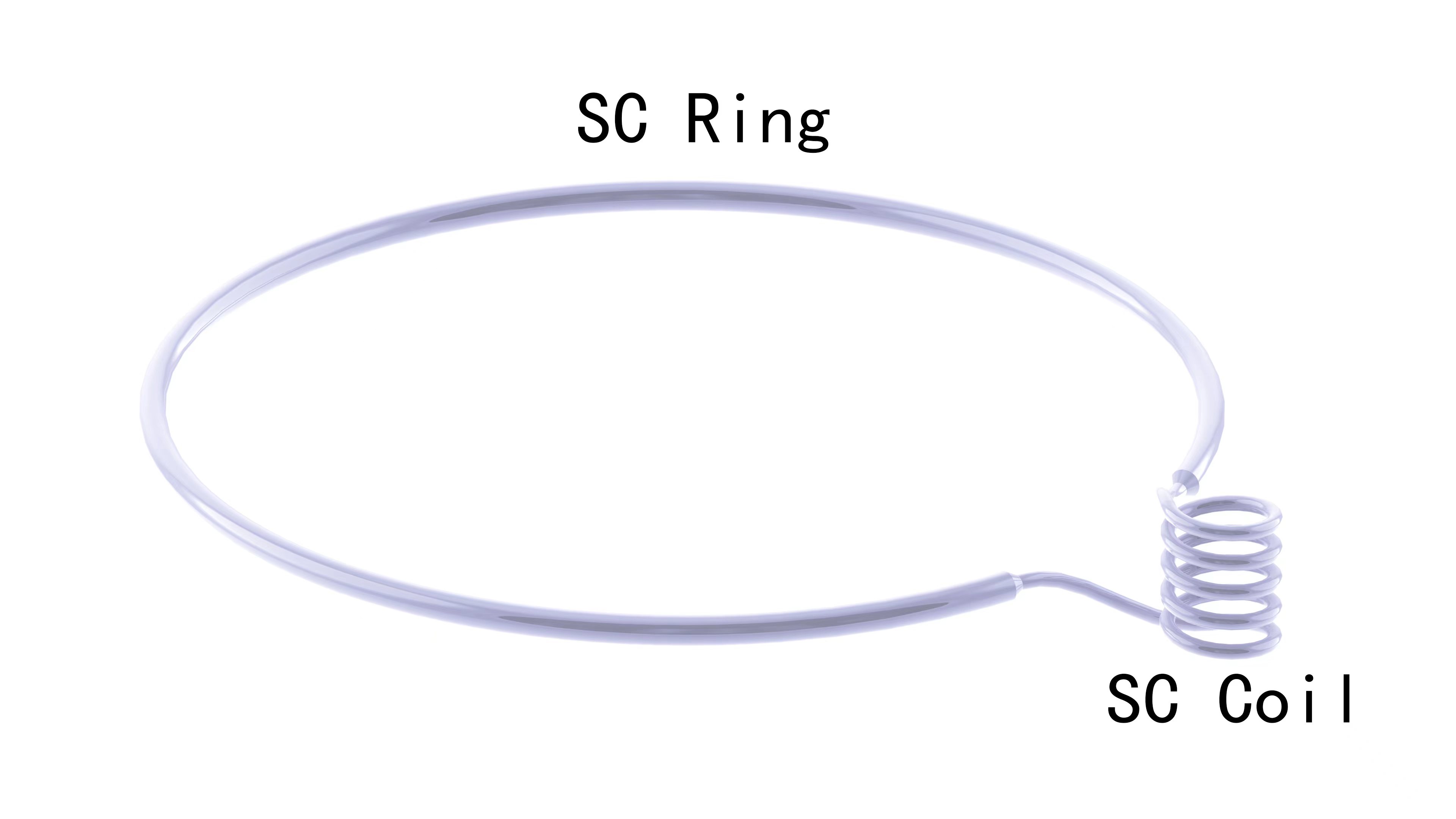
Figure 2: Enhancement of the oscillating $B$-field signal can be achieved by using a superconductor ring-coil pickup. A superconductor ring couples to an $N$ turn coil, and then the magnetic field is boosted by $N*r_{2}/r_{1}$, where $N$ is the turning of the coil. Compared to an LC circuit, a ring-coil maintains a large bandwidth and does not need to be tuned to the dark matter axion frequency.

II Theoretical considerations and a preliminary setup

The dark matter axions can be considered free streaming particles on the laboratory scale. In addition, the cold dark matter particles are nonrelativistic; therefore, the local axion field can be written as:

$$a(x)\approx a_{0}{\rm cos}\left(-m_{a}t-{m_{a}\over 2}v^{2}t+m_{a}\vec{v}\cdot\vec{x}+\phi_{0}\right)~{},$$ (3)

where $a_{0}\approx\sqrt{2\rho_{CDM}}/m_{a}$ is the averaged axion field strength, $\rho_{CDM}$ is the local dark matter energy density, $v$ is the local dark matter velocity relative to the laboratory, which we will take $v\approx 3\times 10^{-3}$c, as the weakly interacting particles should have a speed similar to the sun in the galaxy gravitational well. $\phi_{0}$ is a phase factor and can be safely neglected in the following discussion. The one-half of the axion de-Broglie wavelength is ($\hbar=1$)

$${\lambda\over 2}={\pi\over m_{a}v}\approx 20.9{\rm~{}meter}\cdot\left({10^{-5}{\rm eV}\over m_{a}}\right)~{}~{}.$$ (4)

Thus, when the axions have a mass smaller than $10^{-5}$eV, the field is effectively homogeneous in the laboratory.

The axion couples to the photon via Eq.(1), which gives rise to additional terms in the equations of motion:

$$\vec{\nabla}\cdot\vec{E} = \rho_{e}+g_{a\gamma}\vec{B}\cdot\nabla a$$

$$\vec{\nabla}\times\vec{B}-{\partial\vec{E}\over\partial t} = g_{a\gamma}\vec{E}\times\vec{\nabla}a-g_{a\gamma}\vec{B}{\partial a\over\partial t}+\vec{j}_{e}$$

$$\vec{\nabla}\cdot\vec{B} = 0$$

$$\vec{\nabla}\times\vec{E} = -{\partial\vec{B}\over\partial t}~{},$$ (5)

where $\rho_{e}$ and $\vec{j}_{e}$ are the ordinary electric charge density and current density, respectively. When a static electric field strength $\vec{E}_{0}$ is present, the oscillating axion field induces a small magnetic field and, up to the first order of $g_{a\gamma}$, satisfies

$$\vec{\nabla}\times\vec{B}=g_{a\gamma}(\vec{E}_{0}\times\vec{v})\sqrt{2\rho_{CDM}}{\rm cos}\left[m_{a}(1+{1\over 2}v^{2})t\right]=\vec{j}_{a}~{},$$ (6)

where we have assumed that the electric field permeated region is smaller than the de Broglie wavelength of the dark matter axions. Eq.(6) resembles Ampere’s law with an axion-induced effective current density $\vec{j}_{a}$.

The dark matter axions have a small velocity distribution $\delta v$, which depends on the effective dark matter temperature $T$. The axions are generally very cold, resulting in a typical $\delta v\lesssim 10^{-7}$c Sikivie:2001fg ; Armendariz-Picon:2013jej . The velocity distribution gives rise to an inherent frequency bandwidth:

$$\delta f_{a} = {\delta E\over 2\pi}={m_{a}v\over 2\pi}\delta v\sim 0.5*10^{-10}m_{a}$$ (7)

$$\sim 0.75{\rm Hz}\left({m_{a}\over 10^{-5}{\rm eV}}\right).$$

We can define $Q_{a}={f_{a}/\delta f_{a}}\approx 3*10^{9}$. $Q_{a}$ is the inherent quality factor of the axion dark matter.

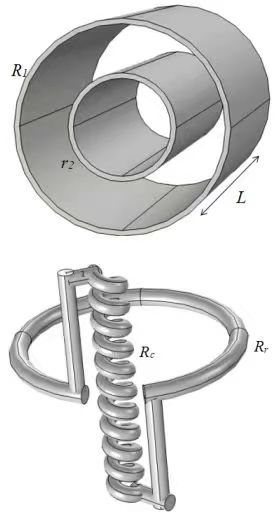
Figure 3: A COMSOL modeling of the cylinder capacitor and the pickup coil.

$R_{1}$	1m	The outer radius of the shell of the cylinder
$r_{2}$	0.5m	The outer radius of the inner shell of the cylinder
$\Delta R,~{}\Delta r$	0.05m	The thickness of the shells
$L$	5m	The height of the cylinder
$R_{r}$	0.365m	The radius of the ring
$R_{c}$	0.04m	The radius of the coil
$N$	10.6	The number of coil turns
The Cylindrical Shell	Material	Solid Silicon
Ring	Material	Gold
Coil	Material	Gold
Other Areas	Material	Air
Boundary	Without *	Air
Boundary	With *	Copper shell

Table 1: The simulation parameters.

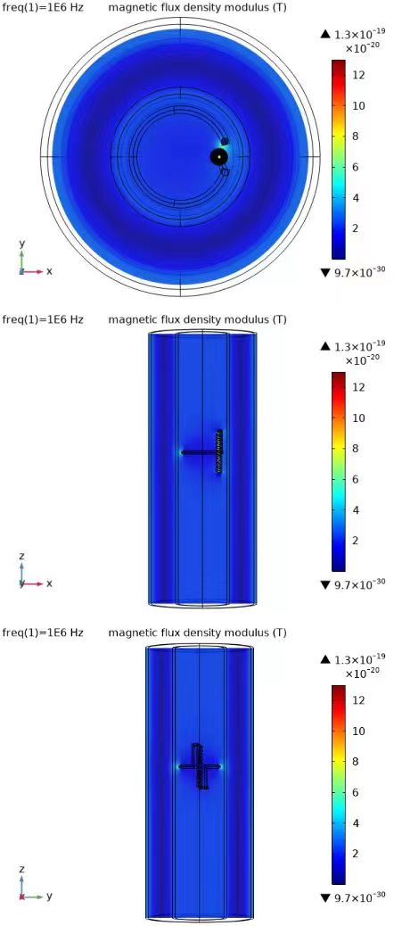
Figure 4: EM simulation of the proposed scheme with the axion frequency at 1 MHz.

Please see Fig. (1), Fig. (2) and Fig. (3) for a preliminary experimental setup. A cylindrical capacitor can be an ideal device to create a confined region with a strong electric field $\vec{E}_{0}$. Assuming the axile length $L$ is much larger than the radius of the cylinder, when the axion velocity $v$ is parallel to the axile, the induced effective current density $\vec{j}_{a}$ runs a closed cycle that lies in the cross-section of the cylinder. Consequently, the induced magnetic field strength $\vec{B}_{a}$, similar to a solenoid case, points along with the cylinder axis. Some portion of $j_{a}$ can be parallel to the cylinder axis when the axion velocity is partially perpendicular to the cylinder axis. The axion induced magnetic field strength is

$$B_{a} =\mu_{0}Rj_{a}=g_{a\gamma}\bar{E}_{0}v\sqrt{2\rho_{CDM}}R{\rm cos}(\omega_{a}t)$$ (8)

$$= 2.0\times 10^{-7}{\rm T}\left({g_{a\gamma}\over{\rm GeV^{-1}}}\right)\left({\bar{E}_{0}\over{\rm Gvolt/m}}\right)\left({R\over{\rm 1m}}\right)$$

$$\times {\rm cos}(\omega_{a}t)$$

where $R$ is the distance between the two plates of the capacitor. Practically, the electric field $E_{0}$ is constrained by the field emission phenomena, and $R$ is constrained by the axion de Broglie wavelength. Note that this result should be taken as an estimation of the order of magnitude of the signals. In an actual experimental setup, one must consider the boundary condition imposed by a particular apparatus and the perturbation corrections due to the induced dynamic electric field component. Fortunately, in very light mass axion searches, the extremely small induced signal and its slow variation make materials respond weakly. We used the COMSOL package to perform 3D electromagnetic simulation for the experimental scheme with specific materials and axion frequencies, with our geometric layout shown in Fig. 3 and configurations listed in Table 1. We find that the simulated signal $B_{a}$ field strength in the inner region agrees with Eq. 8 toward low frequency; see Table 2. At higher frequencies, the screening due to the inner surface causes a larger suppression. One simulation sample is shown in Fig. 4. For additional simulation results at different axion frequencies and with exterior shielding, see Appendix A.

Freq.	Eq. 8 (T)	$B_{a}$ (T)	$B_{1}$ (T)	$F_{r}$
50 Hz	$6.36\times 10^{-20}$	$2.13\times 10^{-20}$	$1.09\times 10^{-19}$	0.053
50 Hz*	$6.36\times 10^{-20}$	$3.18\times 10^{-20}$	$1.75\times 10^{-19}$	0.057
1 MHz	$6.36\times 10^{-20}$	$1.86\times 10^{-20}$	$1.3\times 10^{-19}$	0.072
1 MHz*	$6.36\times 10^{-20}$	$2.57\times 10^{-20}$	$2.01\times 10^{-19}$	0.081
10 MHz	$6.36\times 10^{-20}$	$5.51\times 10^{-21}$	$4.13\times 10^{-20}$	0.077
10 MHz*	$6.36\times 10^{-20}$	$5.52\times 10^{-21}$	$4.18\times 10^{-20}$	0.078

Table 2: Comparisons between Eq. 8 and simulation results. $B_{1}$ is the amplified signal field strength inside the pickup coil. Due to computational power limits, we simulated for $M_{B}\sim 10$. The superscript $*$ denotes simulations with a copper shell as a boundary for the experimental low-temperature environment.

The axion-induced magnetic field $B_{a}$ can be measured by a SQUID-based magnetometer. The sensitivity of such a device is approximately $\Delta B\approx B_{0}*\sqrt{\Delta f/{\rm Hz}}$ Tesla, where $\Delta f$ is the bandwidth of the signal of interest. Due to Eq.(7) and the fact that the low mass axions allow a larger $R$, the proposed scheme is more suitable for lighter axions.

$B_{a}$ permeates the inner part of the capacitor; thus, there are several ways to boost the signal. One can put a superconductor ring with a small coil inside the inner region to achieve an order of $F_{r}*N(R_{r}/R_{c})B_{a}$ enhancement, where $R_{r}$ is the diameter of the superconductor ring. $R_{c}$ is the diameter of the coil, $N$ is the winding number of the coil and $F_{r}$ is a form factor of the ring-coil system depending on the particular design. Please see Fig.(2,3) for an illustration. The coil induces a magnetic field:

$$B_{1}\approx F_{r}N\left({r_{2}\over r_{1}}\right)B_{a}=M_{B}B_{a}~{},$$ (9)

and the boosted signal’s bandwidth remains the same as that of the dark matter axion. Here, we use $M_{B}$ to denote the boost factor, which can be on the order of $10^{4}$ for a modest setup.

III sensitivity forecast

The noise of the experiment mainly comes from the thermal noise in the pickup and the magnetometer. With a superconducting pickup coil, the major source of white noise is the SQUID itself. Here, we will adopt the sensitivity in the frequency range dominated by the SQUID’s white noise, where low-frequency noise is subdominant and the magnetic field is relatively frequency insensitive. The thermal current fluctuations in a given frequency band $\Delta f$ are $\Delta I=\sqrt{{(4k_{B}T\Delta f)/r}}$, where $k_{B}$ is the Boltzmann constant, $r$ is the total resistance and $T$ is the operating temperature. One can ignore the thermal current on the capacitor plates, as for the plates, the requirement $\Delta I<j_{a}LD$ can be achieved by using low conductivity materials, for example, silicon-like plates. Typically, the temperature of the ring-coil system to be a superconductor is approximately several kelvin, which should be sufficient for the proposed scheme. Certainly, read-out systems such as SQUID sensors could require a lower local working temperature.

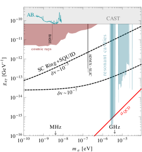
Figure 5: The sensitivity of the axion-photon coupling $g_{a\gamma}$ of the proposed experiment with a preliminary setup $\bar{E}_{0}\sim 10^{3}$MVm^-1, $R\sim 1$m, $\delta v\sim 10^{-3}$, assuming 10 aT magnetic field sensitivity (solid). The limit for a more coherent DM distribution $\delta v\sim 10^{-7}$ is also shown. For comparison, we show the limits from CAST (gray), the collective resonant-cavity haloscope results (green) from ADMX, CAPP, HAYSTAC, etc., plus the recent lower-frequency experimental results from BASE Devlin:2021fpq , ADMX-SLIC Crisosto:2019fcj and ABRACADABRA (AB.) Salemi:2021gck . The red solid line $a_{\rm QCD}$ denotes the prediction from the KSVZ QCD-axion model.

In addition to thermal noise, other potential perturbations to the magnetic field signal include, for instance, electric leakage between the capacitor plates and magnetic environment fluctuations. With proper electric shielding, high-frequency ambient magnetic field fluctuations can be effectively removed. The capacitor’s electric leakage causes a nonperiodic current. Mechanic vibrations need to be screened as low as possible, and they can be calibrated in situgirard2023 . The low-frequency fraction of environmental field fluctuations, such as the Earth’s magnetic field, can be removed by frequency filtering in the dark matter axion’s signal waveband. One major concern could be the breakdown electric-field strength of the capacitor. The electrical breakdown of silver or silver-nickel alloy in a 1.4^-4 Pa vacuum is approximately 2-4$\times 10^{9}$ V/m with negligible leakage current zouache . For semiconductors, Ref. Lin2005 found that the breakdown field strength of ultrathin atomic-layers could be 30 MV/cm. The leakage current density between GaAs and Au is relatively high, approximately $10^{-10}$A/cm², but should not be a concern in vacuum.

Modern SQUID-based magnetometry is developing toward atto-Tesla detection and has reached a magnetic field sensitivity Degen:2017

$$\Delta B\sim 10^{-16}{\rm~{}Tesla}\cdot\sqrt{\Delta f/{\rm Hz}}+\Delta B_{\rm min}~{}~{},$$ (10)

where $\Delta f$ is the bandwidth of the measurement, and we added $\Delta B_{\rm min}$ to denote an effective sensitivity lower bound that saturates the experimental capability. The local dark matter density $\rho_{\rm DM}\approx 0.4$ GeV cm^-3, the dark matter velocity $v\approx 3\times 10^{-3}$, and for $\Delta B$ larger than $\Delta B_{\rm min}$, we have the sensitivity on $g_{a\gamma}$ as

$$g_{a\gamma} = 1.7\times 10^{-13}{\rm GeV}^{-1}\left({1{\rm m}\over{R}}\right)\left({1{\rm GV/m}\over{\bar{E}_{0}}}\right)\left({10^{4}\over M_{B}}\right)$$ (11)

$$\cdot \sqrt{{m_{a}\over 10^{-5}{\rm eV}}{\delta v\over 10^{-7}}}~{}~{},$$

assuming preliminary setup $\bar{E}_{0}\sim 10^{3}$ MVm^-1, $R\sim 1$m. The observation bandwidth assumes the axion energy uncertainty $\Delta f=2m_{a}v\delta v$. The search limits are plotted in Fig. 5 for the current $\Delta B\sim$10 atto-Tesla magnetic field sensitivity (dashed lines) for a conventional DM velocity dispersion $\delta v\sim 10^{-3}$ and a more coherent $\delta v\sim 10^{-7}$ situation for comparison. Searching for low-mass axion is at an advantage due to its narrower frequency bandwidth, yet the limit flattens toward low frequency as $\Delta B$ approaches the experimental sensitivity limit $B_{\rm min}$.

IV Discussions

In this paper, we propose to use a cylindrical capacitor-created static electric field to assist the axion dark matter, inducing an oscillating magnetic field that can be further amplified by adding a superconductor ring-coil system. The deployment of a static electric field with a cylindrical manifold can result in a low noise oscillating magnetic field with increased field strength. The experiment is sensitive to the very light axions because the sensitivity can be additionally improved by increasing the size of the capacitor, as the de-Broglie wavelength of the light axions is large.

Because the effective current depends on the electric field vector across the axion flow vector, the magnitude of the signal can be modulated by adjusting the angle between the axion velocity and the axis direction of the capacitor. A 24-hour modulation is expected with a fixed capacitor orientation due to the Earth’s rotation. When the axion flow is nonparallel to the capacitor axis, a rotational nonsymmetric (around the axis) effective current pattern is generated, which induces a magnetic field signal perpendicular to the axis. The superconducting ring-coil system is a pure induction pickup and thus could offer signal magnification over a wide frequency range.

In addition to SQUID-based magneto-meters, recent developments in spin-based precision measurements, such as Wolf2015 show high potentials in very sensitive magnetic field detections. Such cryogenic detectors with a suitable size can be utilized for signal measurement and may stimulate relative searches.

Acknowledgement We thank Dongning Zheng, Zhihui Peng, Yirong Jin, Man Jiao, Qingjin Xu and Yi Zhou for useful discussions. This work is supported by the National Natural Science Foundation of China (11875148, 12150010) and by the Institute of High Energy Physics, Chinese Academy of Sciences (Y95461A0U2).

Appendix A EM simulations

Here, we illustrate the simulation results for the axion frequency at 10 MHz and a lower 50 Hz with and without a copper boundary: Fig. (6), Fig. (7).

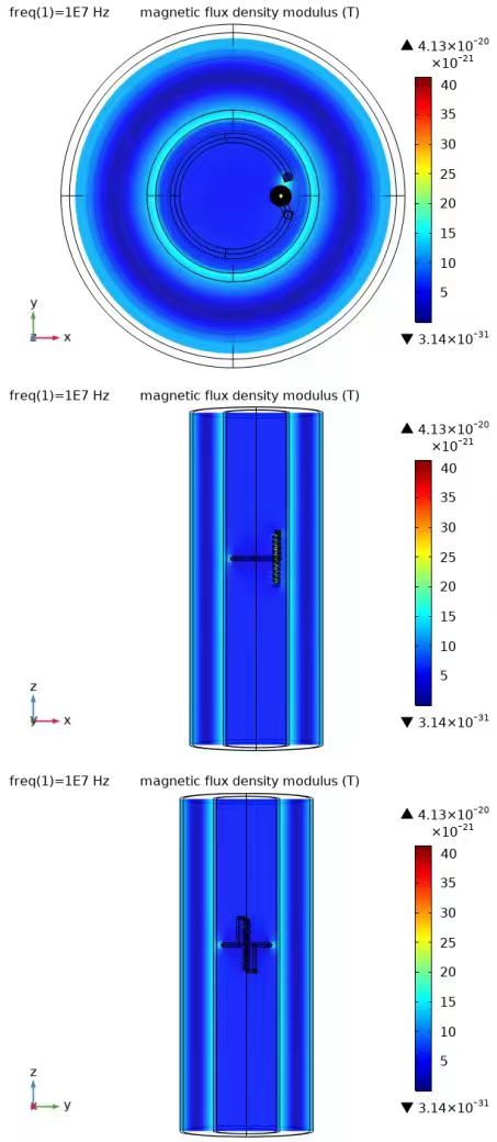
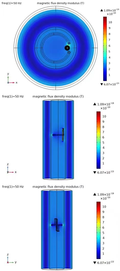
Figure 6: EM simulation of the proposed scheme with axion frequencies of 10 MHz (left) and 50 Hz (right).

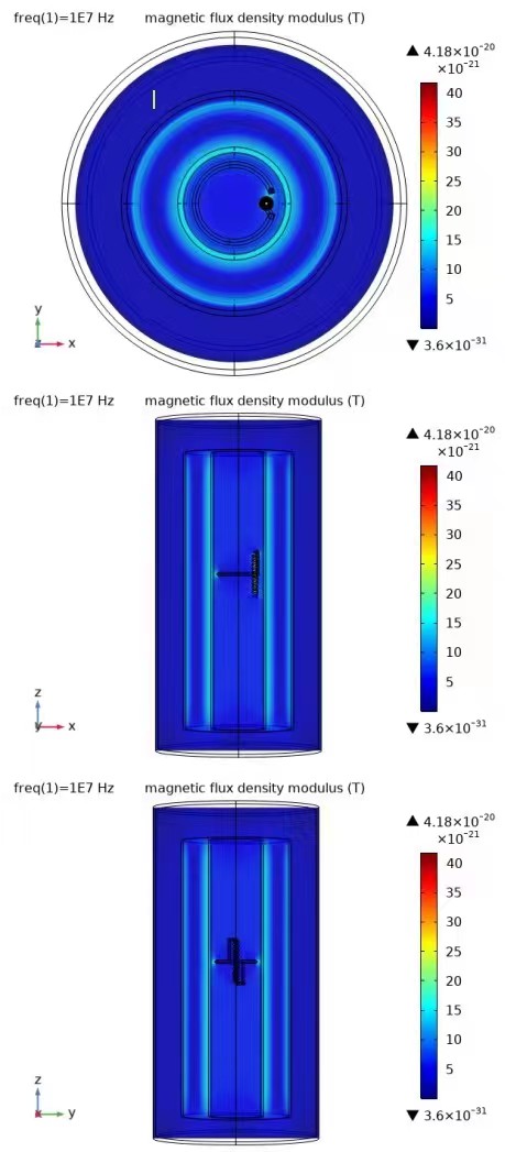
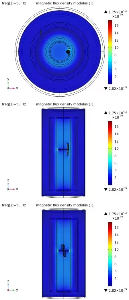
Figure 7: Similar to Fig. 6 but with an exterior copper shield as the boundary of the low-temperature environment.

References

- (1) R. D. Peccei, H. R. Quinn, Phys. Rev. Lett. 38, 1440-1443 (1977).
- (2) R. D. Peccei and H. R. Quinn, Phys. Rev. D 16, 1791 (1977). doi:10.1103/PhysRevD.16.1791
- (3) S. Weinberg, Phys. Rev. Lett. 40, 223 (1978).
- (4) F. Wilczek, Phys. Rev. Lett. 40, 279 (1978).
- (5) M.I.Vysotsky, Ya.B.Zeldovich, M.Yu.Khlopov, and V.M.Chechetkin, ZhETF (1978), V.27, PP. 533-536. [English translation: JETP Lett. (1978) V.27, no.9, PP. 502-505]
- (6) J. E. Kim, Phys. Rev. Lett. 43, 103 (1979).
- (7) M. A. Shifman, A. I. Vainshtein, V. I. Zakharov, Nucl. Phys. B166, 493 (1980).
- (8) A. R. Zhitnitsky, Sov. J. Nucl. Phys. 31, 260 (1980)
- (9) M. Dine, W. Fischler, M. Srednicki, Phys. Lett. B104, 199 (1981).
- (10) A. Davidson and K. C. Wali, Phys. Rev. Lett. 48, 11 (1982). doi:10.1103/PhysRevLett.48.11
- (11) P. Sikivie, Phys. Rev. Lett. 48, 1156 (1982). doi:10.1103/PhysRevLett.48.1156
- (12) L. F. Abbott and P. Sikivie, Phys. Lett. 120B, 133 (1983). doi:10.1016/0370-2693(83)90638-X
- (13) M. Dine and W. Fischler, Phys. Lett. 120B, 137 (1983).
- (14) J. Preskill, M. B. Wise and F. Wilczek, Phys. Lett. 120B, 127 (1983). doi:10.1016/0370-2693(83)90637-8
- (15) J. Ipser and P. Sikivie, Phys. Rev. Lett. 50, 925 (1983). doi:10.1103/PhysRevLett.50.925
- (16) P. Sikivie, Phys. Rev. Lett. 51, 1415 (1983) Erratum: [Phys. Rev. Lett. 52, 695 (1984)]. doi:10.1103/PhysRevLett.51.1415, 10.1103/PhysRevLett.52.695.2
- (17) P. Sikivie, Phys. Rev. D 32, 2988 (1985) Erratum: [Phys. Rev. D 36, 974 (1987)]. doi:10.1103/PhysRevD.36.974, 10.1103/PhysRevD.32.2988
- (18) S. De Panfilis et al., Phys. Rev. Lett. 59, 839 (1987). doi:10.1103/PhysRevLett.59.839
- (19) C. Hagmann, P. Sikivie, N. S. Sullivan and D. B. Tanner, Phys. Rev. D 42, 1297 (1990). doi:10.1103/PhysRevD.42.1297
- (20) Z.G.Berezhiani and M.Yu.Khlopov Yadernaya Fizika (1990) V. 52, PP. 96-103. [English translation: Sov.J.Nucl.Phys. (1990) V. 52, PP.60-64].
- (21) N. Zouache, A. Lefort IEEE Transactions on Dielectrics and Electrical Insulation Vol.4, No.4, 358 (1997).
- (22) W. Hu, R. Barkana and A. Gruzinov, Phys. Rev. Lett. 85, 1158-1161 (2000) doi:10.1103/PhysRevLett.85.1158 [arXiv:astro-ph/0003365 [astro-ph]].
- (23) P. Sikivie, Phys. Lett. B 567, 1-8 (2003) doi:10.1016/S0370-2693(03)00863-3 [arXiv:astro-ph/0109296 [astro-ph]].
- (24) H.C. Lin, P.D. Ye, G.D. Wilk Applied Physics Letters 87, 182904 (2005) doi:10.1063/1.2120904
- (25) P. Svrcek, E. Witten, JHEP 0606, 051 (2006). [hep-th/0605206].
- (26) M. P. Hertzberg, M. Tegmark and F. Wilczek, Phys. Rev. D 78, 083507 (2008) doi:10.1103/PhysRevD.78.083507 [arXiv:0807.1726 [astro-ph]].
- (27) K. Ehret et al., Phys. Lett. B 689, 149 (2010) doi:10.1016/j.physletb.2010.04.066 [arXiv:1004.1313 [hep-ex]].
- (28) H. Tam and Q. Yang, Phys. Lett. B 716, 435 (2012) doi:10.1016/j.physletb.2012.08.050 [arXiv:1107.1712 [hep-ph]].
- (29) D. Wouters et al. [H.E.S.S. Collaboration], arXiv:1304.0700 [astro-ph.HE].
- (30) P. W. Graham and S. Rajendran, Phys. Rev. D 88, 035023 (2013) doi:10.1103/PhysRevD.88.035023 [arXiv:1306.6088 [hep-ph]].
- (31) D. Budker, P. W. Graham, M. Ledbetter, S. Rajendran and A. Sushkov, Phys. Rev. X 4, no. 2, 021030 (2014) doi:10.1103/PhysRevX.4.021030 [arXiv:1306.6089 [hep-ph]].
- (32) P. Sikivie, N. Sullivan and D. B. Tanner, Phys. Rev. Lett. 112, no. 13, 131301 (2014) doi:10.1103/PhysRevLett.112.131301 [arXiv:1310.8545 [hep-ph]].
- (33) C. Armendariz-Picon and J. T. Neelakanta, JCAP 1403, 049 (2014) doi:10.1088/1475-7516/2014/03/049 [arXiv:1309.6971 [astro-ph.CO]].
- (34) Y. V. Stadnik and V. V. Flambaum, Phys. Rev. D 89, no. 4, 043522 (2014) doi:10.1103/PhysRevD.89.043522 [arXiv:1312.6667 [hep-ph]].
- (35) G. Rybka, A. Wagner, A. Brill, K. Ramos, R. Percival and K. Patel, Phys. Rev. D 91, no. 1, 011701 (2015) doi:10.1103/PhysRevD.91.011701 [arXiv:1403.3121 [physics.ins-det]].
- (36) A. Ayala, I. Dominguez, M. Giannotti, A. Mirizzi and O. Straniero, Phys. Rev. Lett. 113, no. 19, 191302 (2014) doi:10.1103/PhysRevLett.113.191302 [arXiv:1406.6053 [astro-ph.SR]].
- (37) P. Sikivie, Phys. Rev. Lett. 113, no. 20, 201301 (2014) doi:10.1103/PhysRevLett.113.201301 [arXiv:1409.2806 [hep-ph]].
- (38) T. Wolf, et al. Phys. Rev. X 5, 041001 (2015)
- (39) Y. Kahn, B. R. Safdi and J. Thaler, Phys. Rev. Lett. 117, no. 14, 141801 (2016) doi:10.1103/PhysRevLett.117.141801 [arXiv:1602.01086 [hep-ph]].
- (40) P. A. R. Ade et al. [Planck], Astron. Astrophys. 594, A13 (2016) doi:10.1051/0004-6361/201525830 [arXiv:1502.01589 [astro-ph.CO]].
- (41) A. Caldwell et al. [MADMAX Working Group], Phys. Rev. Lett. 118 (2017) no.9, 091801 doi:10.1103/PhysRevLett.118.091801 [arXiv:1611.05865 [physics.ins-det]].
- (42) R. Barbieri et al., Phys. Dark Univ. 15, 135 (2017) doi:10.1016/j.dark.2017.01.003 [arXiv:1606.02201 [hep-ph]].
- (43) Q. Yang and H. Di, Phys. Lett. B 780, 622 (2018) doi:10.1016/j.physletb.2018.03.045 [arXiv:1606.01492 [hep-ph]].
- (44) B. M. Brubaker et al., Phys. Rev. Lett. 118, no. 6, 061302 (2017) doi:10.1103/PhysRevLett.118.061302 [arXiv:1610.02580 [astro-ph.CO]].
- (45) C. Abel et al., Phys. Rev. X 7, no. 4, 041034 (2017) doi:10.1103/PhysRevX.7.041034 [arXiv:1708.06367 [hep-ph]].
- (46) V. Anastassopoulos et al. [CAST Collaboration], Nature Phys. 13, 584 (2017) doi:10.1038/nphys4109 [arXiv:1705.02290 [hep-ex]].
- (47) B. T. McAllister, G. Flower, E. N. Ivanov, M. Goryachev, J. Bourhill and M. E. Tobar, Phys. Dark Univ. 18, 67 (2017) doi:10.1016/j.dark.2017.09.010 [arXiv:1706.00209 [physics.ins-det]].
- (48) P. W. Graham, D. E. Kaplan, J. Mardon, S. Rajendran, W. A. Terrano, L. Trahms and T. Wilkason, Phys. Rev. D 97, no. 5, 055006 (2018) doi:10.1103/PhysRevD.97.055006 [arXiv:1709.07852 [hep-ph]].
- (49) D. S. Akerib et al. [LUX Collaboration], Phys. Rev. Lett. 118, no. 26, 261301 (2017) doi:10.1103/PhysRevLett.118.261301 [arXiv:1704.02297 [astro-ph.CO]].
- (50) C.L. Degen, F. Reinhard and P. Cappellaro, Rev. Mod. Phys. 89, 035002 (2017)
- (51) P. W. Graham and A. Scherlis, Phys. Rev. D 98, no.3, 035017 (2018) doi:10.1103/PhysRevD.98.035017 [arXiv:1805.07362 [hep-ph]].
- (52) F. Takahashi, W. Yin and A. H. Guth, Phys. Rev. D 98, no. 1, 015042 (2018) doi:10.1103/PhysRevD.98.015042 [arXiv:1805.08763 [hep-ph]].
- (53) N. Du et al. [ADMX Collaboration], Phys. Rev. Lett. 120, no. 15, 151301 (2018) doi:10.1103/PhysRevLett.120.151301 [arXiv:1804.05750 [hep-ex]].
- (54) L. Zhong et al. [HAYSTAC Collaboration], Phys. Rev. D 97, no. 9, 092001 (2018) doi:10.1103/PhysRevD.97.092001 [arXiv:1803.03690 [hep-ex]].
- (55) L. Visinelli and S. Vagnozzi, Phys. Rev. D 99, no. 6, 063517 (2019) doi:10.1103/PhysRevD.99.063517 [arXiv:1809.06382 [hep-ph]].
- (56) D. J. E. Marsh, K. C. Fong, E. W. Lentz, L. Smejkal and M. N. Ali, Phys. Rev. Lett. 123, no. 12, 121601 (2019) doi:10.1103/PhysRevLett.123.121601 [arXiv:1807.08810 [hep-ph]].
- (57) J. L. Ouellet et al., Phys. Rev. Lett. 122, no. 12, 121802 (2019) doi:10.1103/PhysRevLett.122.121802 [arXiv:1810.12257 [hep-ex]].
- (58) M. Lawson, A. J. Millar, M. Pancaldi, E. Vitagliano and F. Wilczek, Phys. Rev. Lett. 123 (2019) no.14, 141802 doi:10.1103/PhysRevLett.123.141802 [arXiv:1904.11872 [hep-ph]].
- (59) A. Arza and P. Sikivie, Phys. Rev. Lett. 123, no. 13, 131804 (2019) doi:10.1103/PhysRevLett.123.131804 [arXiv:1902.00114 [hep-ph]].
- (60) Q. Yang, [arXiv:1912.11472 [hep-ph]].
- (61) N. Crisosto, P. Sikivie, N. S. Sullivan, D. B. Tanner, J. Yang and G. Rybka, Phys. Rev. Lett. 124, no.24, 241101 (2020) doi:10.1103/PhysRevLett.124.241101 [arXiv:1911.05772 [astro-ph.CO]].
- (62) Y. Gao, T. Li and Q. Yang, [arXiv:1912.12963 [hep-ph]].
- (63) C. Bartram et al. [ADMX], Phys. Rev. Lett. 127, no.26, 261803 (2021) doi:10.1103/PhysRevLett.127.261803 [arXiv:2110.06096 [hep-ex]].
- (64) J. A. Devlin, M. J. Borchert, S. Erlewein, M. Fleck, J. A. Harrington, B. Latacz, J. Warncke, E. Wursten, M. A. Bohman and A. H. Mooser, et al. Phys. Rev. Lett. 126, no.4, 041301 (2021) doi:10.1103/PhysRevLett.126.041301 [arXiv:2101.11290 [astro-ph.CO]].
- (65) C. P. Salemi, J. W. Foster, J. L. Ouellet, A. Gavin, K. M. W. Pappas, S. Cheng, K. A. Richardson, R. Henning, Y. Kahn and R. Nguyen, et al. Phys. Rev. Lett. 127, no.8, 081801 (2021) doi:10.1103/PhysRevLett.127.081801 [arXiv:2102.06722 [hep-ex]].
- (66) J.-P. Girard, R. E. Lake, W. Liu, R. Kokkoniemi, E. Visakorpi, J. Govenius, M. Mottonen, Rev. Sci. Instrum 94, 054710 (2023). doi:10.1063/5.0143761