A $w-M$ phantom transition at $z_{t}<0.1$ as a resolution of the Hubble tension

Abstract

A rapid phantom transition of the dark energy equation of state parameter $w$ at a transition redshift $z_{t}<0.1$ of the form $w(z)=-1+\Delta w\;\Theta(z_{t}-z)$ with $\Delta w<0$ can lead to a higher value of the Hubble constant while closely mimicking a Planck18/$\Lambda$CDM form of the comoving distance $r(z)=\int_{0}^{z}\frac{dz^{\prime}}{H(z^{\prime})}$ for $z>z_{t}$. Such a transition however would imply a significantly lower value of the SnIa absolute magnitude $M$ than the value $M_{C}$ imposed by local Cepheid calibrators at $z<0.01$. Thus, in order to resolve the $H_{0}$ tension it would need to be accompanied by a similar transition in the value of the SnIa absolute magnitude $M$ as $M(z)=M_{C}+\Delta M\;\Theta(z-z_{t})$ with $\Delta M<0$. This is a Late $w-M$ phantom transition ($LwMPT$). It may be achieved by a sudden reduction of the value of the normalized effective Newton constant $\mu=G_{\rm{eff}}/G_{\rm{N}}$ by about $6\%$ assuming that the absolute luminosity of SnIa is proportional to the Chandrasekhar mass which varies as $\mu^{-3/2}$. We demonstrate that such an ultra low $z$ abrupt feature of $w-M$ provides a better fit to cosmological data compared to smooth late time deformations of $H(z)$ that also address the Hubble tension. For $z_{t}=0.02$ we find $\Delta w\simeq-4$, $\Delta M\simeq-0.1$. This model also addresses the growth tension due to the predicted lower value of $\mu$ at $z>z_{t}$. A prior of $\Delta w=0$ (no $w$ transition) can still resolve the $H_{0}$ tension with a larger amplitude $M$ transition with $\Delta M\simeq-0.2$ at $z_{t}\simeq 0.01$. This implies a larger reduction of $\mu$ for $z>0.01$ (about $12\%$). The $LwMPT$ can be generically induced by a scalar field non-minimally coupled to gravity with no need of a screening mechanism since in this model $\mu=1$ at $z<0.01$.

I Introduction

The cosmological comoving distance to redshift $z$ defined in a flat universe as $r(z)=\int_{0}^{z}\frac{dz^{\prime}}{H(z^{\prime})}$ where $H(z)$ is the Hubble expansion rate has been constrained to a level of about $2\%$ using standard candles (SnIa calibrated with Cepheid stars Riess et al. (2019, 2018, 2016) and Red Giant stars Freedman et al. (2020, 2019) or megamasers in accretion disks Pesce et al. (2020)), a standard ruler (the sound horizon at last scattering calibrated using the CMB anisotropy spectrum Aghanim et al. (2020); Addison et al. (2018) and/or Big Bang Nucleosynthesis (BBN) Schöneberg et al. (2019)), strong gravitational lensing Birrer et al. (2019); Shajib et al. (2020) and gravitational waves Abbott et al. (2019); Soares-Santos et al. (2019). The comoving distance determined using calibrated standard candles at $z<0.1$ is offset with the comoving distance determined using the sound horizon standard ruler at $z>0.1$, by about $9\%$ which corresponds to a tension of about $5\sigma$. In the context of a Planck18/$\Lambda$CDM form of $H(z)$ this mismatch of $r(z)$ becomes realized as a mismatch of the values of the Hubble constant determined by the two methods Knox and Millea (2020); Mörtsell and Dhawan (2018).

Despite of intense efforts Efstathiou (2020); Kazantzidis and Perivolaropoulos (2020); Kazantzidis et al. (2020); Sapone et al. (2020) it has not been possible to reliably identify systematic errors of the calibrators used in the context of the two methods. For example parallax data from Gaia have recently confirmed Soltis et al. (2020); Riess et al. (2020) the calibration of Cepheid stars while attempts to recalibrate the sound horizon assuming e.g. neutrino self interactions Blinov et al. (2019), early dark energy Poulin et al. (2019); Sakstein and Trodden (2020); Agrawal et al. (2019); Lin et al. (2019); Braglia et al. (2020); Niedermann and Sloth (2020); Smith et al. (2020a) or modified gravity Benisty (2019); Ballardini et al. (2020) have either failed to significantly reduce the tension level Ballardini et al. (2020); D’Amico et al. (2020) or produced new tensions with other cosmological data Haridasu et al. (2020); Krishnan et al. (2020a) (including growth rate from weak lensing Hildebrandt et al. (2017); Joudaki et al. (2018); Köhlinger et al. (2017); Abbott et al. (2018) and peculiar velocities Macaulay et al. (2013); Kazantzidis and Perivolaropoulos (2018); Nesseris et al. (2017); Skara and Perivolaropoulos (2020); Kazantzidis and Perivolaropoulos (2019); Kazantzidis et al. (2019)). It therefore becomes increasingly probable that the mismatch in the high-z -low-z form of $r(z)$ is indeed a physical effect Di Valentino et al. (2021) that will require deformation of $H(z)$ from its Planck18/$\Lambda$CDM form and/or some other modification of late time physics.

Attempts to consider smooth deformations of $H(z)$ Alestas et al. (2020); Di Valentino et al. (2016); Smith et al. (2020b); Vagnozzi (2020); Li and Shafieloo (2019); Di Valentino et al. (2020); Krishnan et al. (2020b) at $z\simeq O(1)$ have been successful in matching $r(z_{rec})$ with $r(z=0)$ but have been unable to match the value of $r(z\simeq O(1))$ which is strongly constrained by BAO and SnIa data to be close to the form indicated by Planck18/$\Lambda$CDM.

A remaining possibility is that of an abrupt deformation of $H(z)$ at $z\lesssim 0.1$ ($H(z)$ transition). Such a deformation has been considered in previous studies Mortonson et al. (2009); Benevento et al. (2020); Dhawan et al. (2020) as a discontinuity of $H(z)$ occurring at $z_{t}<0.1$. It was shown however, that if such a feature occurs at $z_{t}<0.01$ i.e. below the redshift where Hubble flow starts, it would be undetectable by standard candles Benevento et al. (2020) and thus it would not be able to justify the measured decreased value of $r(z)$ at low $z$. On the other hand, if it occurred at $0.01<z_{t}<0.1$ with the proper amplitude to reduce $r(z)$ to the required level, it would have to produce a step-like feature in the SnIa Hubble diagram with amplitude $\Delta m=0.2$. A discontinuity with such an amplitude is inconsistent with the Pantheon data. It is therefore clear that even though the existence of a feature in the form of $H(z)$ at $z_{t}<0.1$ is likely, this feature is severely constrained by both the constraints on the comoving distance $r(z)$ at $z>0.1$ as well as by the measured SnIa magnitudes which are not consistent with a large step-like discontinuity. This problem can be avoided by assuming a transition of the SnIa absolute magnitude $M$ at $z_{t}\in[0.01,0.1]$ which can nullify the required step-like feature of the apparent magnitudes while being consistent with value of the absolute magnitude implied by local Cepheid calibrators. In the present analysis we propose such a feature in the form of a a transition of the SnIa absolute magnitude accompanied by transition of the equation dark energy of state parameter $w(z)\equiv\frac{p_{de}(z)}{\rho_{de}(z)}$ Keeley et al. (2019); Bassett et al. (2002).

In particular, we consider a transition of $w(z)$ as

$$w(z)=-1+\Delta w\;\Theta(z_{t}-z)$$ (1)

while also allowing for a corresponding transition for the SnIa absolute magnitude $M$ (due to fundamental physics changes that accompany the $w$ transition) of the form

$$M(z)=M_{C}+\Delta M\;\Theta(z-z_{t})$$ (2)

where $\Theta$ is the Heaviside step function, $M_{C}=-19.24$ is the SnIa absolute magnitude calibrated by Cepheids Camarena and Marra (2021, 2020) at $z<0.01$ and $\Delta M$, $\Delta w$ are parameters to be fit by the data.

The equation of state parameter determines the gravitational properties and the evolution of dark energy density $\rho_{de}$. From energy momentum conservation $d(\rho_{de}a^{3})=-p_{de}d(a^{3})$ it is easy to show that the evolution of dark energy density is obtained as

$$\rho_{de}(z)=\rho_{de}(z_{p})\int_{z_{p}}^{z}\frac{dz^{\prime}}{1+z^{\prime}}(1+w(z^{\prime}))=\rho_{de}(z_{p})\left(\frac{1+z}{1+z_{p}}\right)^{3(1+w)}$$ (3)

where in the last equality a constant $w$ was assumed and $z_{p}$ is a pivot redshift which may be assumed equal to the present time or equal to the transition time $z_{t}$. Eqs. (1) and (3) imply a continuous Hubble expansion rate $h(z)\equiv H(z)/100km/(sec\cdot Mpc)$ of the form

$$h_{w}(z)^{2} \equiv\omega_{m}(1+z)^{3}+\omega_{r}(1+z)^{4}+(h^{2}-\omega_{m}-\omega_{r})\left(\frac{1+z}{1+z_{t}}\right)^{3\;\Delta w} z<z_{t}$$ (4)

$$h_{w}(z)^{2} \equiv\omega_{m}(1+z)^{3}+\omega_{r}(1+z)^{4}+(h^{2}-\omega_{m}-\omega_{r}) z>z_{t}$$

where $\omega_{m}\equiv\Omega_{0m}h^{2}$, $\omega_{r}\equiv\Omega_{0r}h^{2}$ are the matter and radiation density parameters assumed fixed to their Planck18/$\Lambda$CDM values in the next section and $h$ is a parameter distinct from the rescaled measurable Hubble parameter $h_{w}(z=0)$. In what follows we assume $0.01<z_{t}<0.1$ and define $h_{local}\equiv 0.74$ and $h_{CMB}\equiv 0.674$ which correspond to the Hubble constant values obtained with local standard candle measurements of $r(z)$ ($H_{0}=H_{0}^{R19}$) and sound horizon standard ruler measurements ($H_{0}=H_{0}^{P18}$ calibrated by Planck18/$\Lambda$CDM) respectively.

In the context of the above Late $w-M$ Phantom Transition ($LwMPT$) model the following interesting questions emerge:

• What is the functional form of $\Delta w(z_{t})$ so that $h_{w}(z=0)=h_{local}$ as implied by local measurements while maintaining the required Planck18/$\Lambda$CDM form of $r(z)$ for $z\gg z_{t}$?

• How closely does the $LwMPT$ model reproduce the form of the Planck18/$\Lambda$CDM comoving distance $r(z)$ for $z>z_{t}$? How does this form of $r(z)$ compare with the corresponding form of the $H(z)$ transition?

• How does the quality of fit of the $LwMPT$ model to cosmological data (CMB, SnIa, BAO and SH0ES) compare with the corresponding quality of fit of typical models that utilize smooth deformations of $H(z)$ to address the $H_{0}$ tension?

• What are the favored values of $\Delta w$, $\Delta M$ and what are the implications for general relativity and for the future evolution of the universe?

In the present analysis we address the above questions. The structure of this paper is the following: In the next section we investigate analytically the ability of the $LwMPT$ model (4) to reproduce the Planck18/$\Lambda$CDM form of the comoving distance for $z>z_{t}$ while keeping $h_{w}(z=0)=0.74$. We also identify the values $\Delta w(z_{t})$ that achieve this goal using an analytical approach. In section III we use cosmological data (CMB, SnIa, BAO and SH0ES) to identify the best fit parameter values for various transition redshifts $z_{t}$ and identify the improvement of the quality of fit as $z_{t}$ decreases down to the minimum acceptable value $z_{t}\simeq 0.02$. We also compare this quality of fit to the data with the Planck18/$\Lambda$CDM model (without the SH0ES datapoint) and with a typical smooth $H(z)$ deformation model ($wCDM$) that is designed to address the Hubble tension. Finally in section IV we summarize the main results of our analysis and discuss the implications of these results for the future evolution of the universe if this model is indeed realized in Nature. We also discuss possible future extensions of this analysis.

II The cosmological comoving distance in the $LwMPT$ model

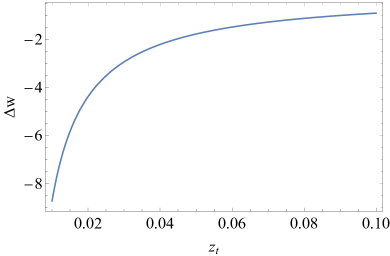
Figure 1: The equation of state shift $\Delta w$ required for $h_{w}(z=0)=h_{local}$ as a function of the transition redshift $z_{t}$. Notice the strongly phantom behavior of the dark energy equation of state $w=-1-\Delta w$ for $z<z_{t}$.

In order to fix the parameters $\omega_{m}$, $\omega_{r}$, $h$ and $\Delta w$ in the $LwMPT$ ansatz (4) we impose the following conditions:

• It should reproduce the comoving distance corresponding to Planck18/$\Lambda$CDM $r_{\Lambda}$ for $z\gg z_{t}$ where

  $$r_{\Lambda}(z)\equiv\int_{0}^{z}\frac{dz^{\prime}}{\omega_{m}(1+z^{\prime})^{3}+\omega_{r}(1+z^{\prime})^{4}+(h^{2}-\omega_{m}-\omega_{r})}$$ (5)

  where $\omega_{m}\equiv\Omega_{0m}h^{2}=0.143$, $\omega_{r}\equiv\Omega_{0r}h^{2}=4.64\times 10^{-5}$ and $h=h_{CMB}=0.674$.

• It should reproduce the local measurements of the Hubble parameter

  $$h_{w}(z=0)=h_{local}=0.74.$$ (6)

The first condition fixes the parameters $\omega_{m}$, $\omega_{r}$ and $h$ to their Planck18/$\Lambda$CDM best fit values. Since we consider $z_{t}<0.1\ll 1$ it is straightforward to obtain an upper bound for the relative difference

$$\frac{\Delta r}{r}(z)\equiv\frac{r_{w}(z)-r_{\Lambda}(z)}{r_{\Lambda}(z)}<\frac{h_{local}-h_{CMB}}{h_{CMB}}\simeq 0.1$$ (7)

where $r_{w}(z)\equiv\int_{0}^{z}\frac{dz^{\prime}}{h_{w}(z^{\prime})}$ is the comoving distance corresponding to the $LwMPT$ model (4). $\frac{\Delta r}{r}(z)$ is maximum at $z=0$ and decreases rapidly as $z$ increases as demonstrated below.

The second condition imposes the constraint (6) on eq. (4) and leads to a relation between $\Delta w$ and $z_{t}$ of the form (here we neglect $\omega_{r}$ as it has practically no effect on $\Delta w$)

$$\Delta w=\frac{Log\left(h^{2}-\omega_{m}\right)-Log\left(h_{local}^{2}-\omega_{m}\right)}{3Log(1+z_{t})}$$ (8)

where $h=h_{CMB}=0.674$ and $\omega_{m}=\Omega_{0m}h^{2}=0.143$ as implied by the first condition and for consistency with the CMB anisotropy spectrum. In Fig. 1 we show a plot of $\Delta w(z_{t})$ demonstrating the strongly present day phantom behavior of dark energy implied by this class of models.

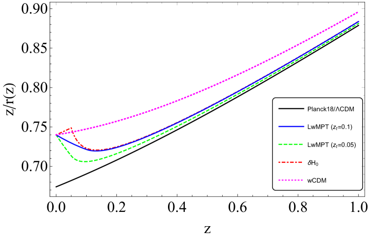
Figure 2: The function $f(z)=z/r(z)$ where $r(z)$ is the comoving distance to redshift $z$ for the cosmological models Planck18/$\Lambda$CDM (black continuous line), $wCDM$ with $w=-1.2$ (magenta dotted line), $H(z)$ transition (9) with $z_{t}=0.05$ and $\frac{\delta h}{h}=(h_{local}-h_{CMB})/h_{CMB}$ (red dot-dashed line), $LwMPT$ with $z_{t}=0.05$ and $w(z<z_{t})=-1-\Delta w=-2.78$ as indicated by eq. (8) (green dashed line) and $LwMPT$ with $z_{t}=0.1$ and $w(z<z_{t})=-1-\Delta w=-1.91$ as indicated by eq. (8) (blue continuous line). Notice that even though all three models approach $r_{\Lambda}(z)$ asymptotically, the two $LwMPT$ models remain closest to the Planck18/$\Lambda$CDM comoving distance $r_{\Lambda}(z)$ while at the same time they are consistent with the local measurement of the Hubble constant since $h_{w}(z=0)=0.74$.

It is of interest to compare the form of the comoving distance $r(z)$ predicted in the context of the $LwMPT$ model $r_{w}(z)$ with other proposed $H(z)$ deformations for the resolution of the Hubble tension. In Fig. 2 we show a plot of the function $f(z)\equiv z/r(z)$ (whose $z\rightarrow 0$ limit is the Hubble constant) for three proposed $H(z)$ deformation resolutions of the Hubble tension: the $LwMPT$ model, the $H(z)$ transition model and the $wCDM$ with fixed $w=-1.22$ model Alestas et al. (2020); Di Valentino et al. (2016); Vagnozzi (2020). The $H(z)$ transition model is defined as

$$h_{\delta}(z)^{2}\equiv(1+\frac{\delta h}{h}\;\Theta(z_{t}-z))^{2}\left[\omega_{m}(1+z)^{3}+\omega_{r}(1+z)^{4}+(h^{2}-\omega_{m}-\omega_{r})\right]$$ (9)

where $\frac{\delta h}{h}=\frac{h_{local}-h_{CMB}}{h_{CMB}}$, $h=h_{CMB}$ and $\omega_{m}$, $\omega_{r}$ are assumed fixed to their Planck18/$\Lambda$CDM best fit values. The fixed $w$ ($wCDM$) smooth $H(z)$ deformation model is defined as

$$h_{wf}(z)^{2}\equiv\omega_{m}(1+z)^{3}+\omega_{r}(1+z)^{4}+(h^{2}-\omega_{m}-\omega_{r})(1+z)^{3(1+w)}$$ (10)

where $w=-1.22$, $h=h_{local}$ and $\omega_{m}$, $\omega_{r}$ are assumed fixed to their Planck18/$\Lambda$CDM best fit values Alestas et al. (2020).

All three models that address the $H_{0}$ tension shown in Fig. 2 satisfy by construction two necessary conditions

$$h(z=0)=h_{local}$$ (11)

$$r(z)\rightarrow r_{\Lambda}(z)\;\;for\;\;z\gtrsim O(1).$$ (12)

These conditions along with the fact that we fix the parameters $\omega_{m}$ and $\omega_{r}$ to their best fit $\Lambda$CDM values secure the fact that all three models produce the same CMB anisotropy spectrum as Planck18/$\Lambda$CDM while at the same time they predict a Hubble parameter equal to its locally measured value $h(z=0)=h_{local}$. However, the three models do not approach the Planck18/$\Lambda$CDM comoving distance $r_{\Lambda}(z)$ with the same efficiency as $z$ increases. As is clearly seen in Fig. 2, the $LwMPT$ model with both $z_{t}=0.1$ and $z_{t}=0.05$ approaches $r_{\Lambda}(z)$ faster than the other two models. Since Planck18/$\Lambda$CDM provides an excellent fit to most geometric cosmological probes at $z>0.1$ it is anticipated that $LwMPT$ will produce a better fit to cosmological data than the smooth deformations of $H(z)$ like $wCDM$ or the discontinuous $H(z)$ transition model which produces an unnatural step in $r(z)$ and moves away from $r_{\Lambda}(z)$ for $z<z_{t}$ as $z$ increases. This improved quality of fit is also demonstrated in the next section.

Any $H(z)$ deformation models that address the Hubble tension should not only be consistent with the locally measured value of the Hubble parameter $H_{0}$ and with the Planck18/$\Lambda$CDM form of $H(z)$. It should also be consistent with the value $M_{C}$ of the absolute magnitude of SnIa as determined by Cepheid calibrators Camarena and Marra (2021, 2020). This may be seen by considering the equation that connects the SnIa measured apparent magnitudes at redshift $z_{i}$ with the Hubble free luminosity distance and the Hubble parameter which may be written as

$$m(z_{i})=M-5\log_{10}\left[H_{0}\cdot{\text{Mpc}/c}\right]+5\log_{10}(D_{L}(z_{i}))+25$$ (13)

where $D_{L}(z)=H_{0}\,d_{L}(z)/c$ is the Hubble free luminosity distance. Given the measured $m(z_{i})$ datapoints the best fit Hubble parameter in the context of local measurements can decrease to become consistent with the sound horizon calibrator by either decreasing $D_{L}(z)$ (deforming $H(z)$) or by decreasing the absolute magnitude $M$. Such a decrease of $M$ can be achieved either by discovering a systematic effect of the Cepheid calibrators or by assuming an $M$ transition at $z\geq 0.01$ due to an abrupt change of fundamental physics. The deformation of $D_{L}(z)$ is severely constrained by the standard ruler constraints based on the sound horizon (CMB and BAO) and even though it is most efficient in the context of very late transitions as the one discussed in the present analysis it may still not be enough to compensate with the decrease of $H_{0}$ while keeping $M$ fixed to its Cepheid calibrated value $M=M_{C}$. A common error made in late time approached of the Hubble tension is to either marginalize over $M$ with a flat prior or allow it to vary along with the cosmological parameters in the context of the maximum likelihood method. This may lead to a best fit value of $M$ that is inconsistent with the Cepheid measured value $M_{C}$ thus invalidating the results of such analysis. This problem may be overcome by allowing for a transition of $M$ from its measured value $M_{C}$ at $z<z_{t}\simeq 0.01$ to a value lower than $M_{C}$ by $\Delta M\geq-5\log_{10}\left[\frac{H^{\rm R19}_{0}}{H^{\rm P18}_{0}}\right]\simeq-0.2$ at $z>z_{t}\simeq 0.01$. Thus in the next section we allow $M$ to vary along with the cosmological parameters in order to achieve a good fit to the data and at the end we determine the required magnitude of the $M$ transition assumed to take place at the same time as the $w$ transition $z=z_{t}$ in the context of a common physical origin. Note however that for $\Delta M=-5\log_{10}\left[\frac{H^{\rm R19}_{0}}{H^{\rm P18}_{0}}\right]\simeq-0.2$ the $M$ transition may be sufficient for the resolution of the $H_{0}$ tension with no need for a $w$ transition.

III Fitting $LwMPT$ to cosmological data and comparison with $wCDM$

In this section we use a wide range of cosmological data to estimate the quality of fit and the best fit parameter values of three representative cosmological models:

• The $LwMPT$ class of models defined by a Hubble expansion rate similar to that of eq. (4). Here we remove the constraint $w_{>}=-1$ for $z>z_{t}$ as well as the constraint $\omega_{m}=0.143$. Thus the model is now allowed to have three free parameters for each fixed value of $z_{t}$: $w_{>}$, $w_{<}\equiv w_{>}+\Delta w$ and $\omega_{m}$. However, as discussed below, the additional free parameters end up constrained by the data very close to the values considered fixed in the previous section. The constraint $h(z=0)=h_{local}$ is imposed as a prior in the analysis.

• The $wCDM$ model defined in (10) with two free parameters: $w$ and $\omega_{m}$. The constraint $h(z=0)=h_{local}$ is imposed as a prior in the analysis.

• The $\Lambda$CDM model defined by (10) with $w=-1$. No constraint for $h(z=0)$ is imposed on this model in order to maximize the quality of fit to the data and use the model as a benchmark for comparison with the other models that address the $H_{0}$ tension. Thus we use the term u$\Lambda$CDM (“u” for “unconstrained”) to denote it. It is considered as a baseline to compute residuals of $\chi^{2}$ to compare the other two representative models. Its best fit parameter values ($\Omega_{0m}=0.312\pm 0.006,H_{0}=67.579\pm 0.397$) in the context of the dataset we use are almost identical with Planck18/$\Lambda$CDM.

We use the following data to identify the quality of fit of these models

• The Pantheon SnIa dataset Scolnic et al. (2018) consisting of 1048 distance modulus datapoints in the redshift range $z\in[0.01,2.3]$.

• A compilation of 9 BAO datapoints in the redshift range $z\in[0.1,2.34]$. The compilation is shown in the Appendix.

• The latest Planck18/$\Lambda$CDM CMB distance prior data (shift parameter $R$ Elgaroy and Multamaki (2007) and the acoustic scale $l_{a}$ Zhai and Wang (2019)). These are highly constraining datapoints based on the observation of the sound horizon standard ruler at the last scattering surface $z\simeq 1100$. The covariance matrix of these datapoints and their values are shown in the Appendix.

• A compilation of 41 Cosmic Chronometer (CC) datapoints in the redshift range $z\in[0.1,2.36]$. These datapoints are shown in the Appendix and have much less constraining power than the other data we use.

Using these data (total of 1100 datapoints) we used the maximum likelihood method Arjona et al. (2019) to minimize the total $\chi^{2}$ defined as

$$\chi^{2}=\chi^{2}_{CMB}+\chi^{2}_{BAO}+\chi^{2}_{CC}+\chi^{2}_{Panth}$$ (14)

and calculate the residual $\Delta\chi^{2}$ with respect to the u$\Lambda$CDM model for the $LwMPT$ class (as a function of $z_{t}$) and for $wCDM$. Since the CMB data are the most constraining, we have found the anticipated best fits $\omega_{m}\simeq 0.143$ and $w=-1.22$ for $wCDM$ (see Ref. Alestas et al. (2020) for a detailed analysis of these results).

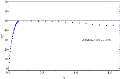
Figure 3: The residuals $\Delta\chi^{2}$ plotted against the values of the transition redshift $z_{t}$ for the $LwMPT$ (blue dots) and $wCDM$ (black dotted line) with $w=-1.22$. The $LwMPT$ model seems to achieve a significantly better fit for small $z_{t}$ values.

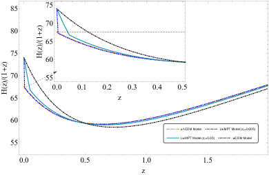
Figure 4: The forms of the comoving Hubble parameter $H(z)/(1+z)$ for two $LwMPT$ models with $z_{t}<0.1$, the best fit $wCDM$ and u$\Lambda$CDM.

In Fig. 3 we show the residuals $\Delta\chi^{2}$ for the best fit $LwMPT$ models as a function of $z_{t}$ (blue points) and the corresponding residual $\Delta\chi^{2}$ for the best fit $wCDM$ model (horizontal black line). As mentioned in the previous section no prior is imposed on $M$ but at the end we will identify the magnitude $\Delta M$ of the required $M$ transition. The rapid improvement of the fit compared to $wCDM$ for the $LwMPT$ models as $z_{t}$ decreases below $z_{t}\simeq 0.15$ is clear. The best fit parameter values for $w_{<}$ ($z<z_{t}$) and $w_{>}$ ($z>z_{t}$) are shown in Table 1. In parenthesis next to each $w_{<}$ best fit we show the predicted value in the context of the analysis of the previous section (eq. (8)) which assumes $w_{>}=-1$.

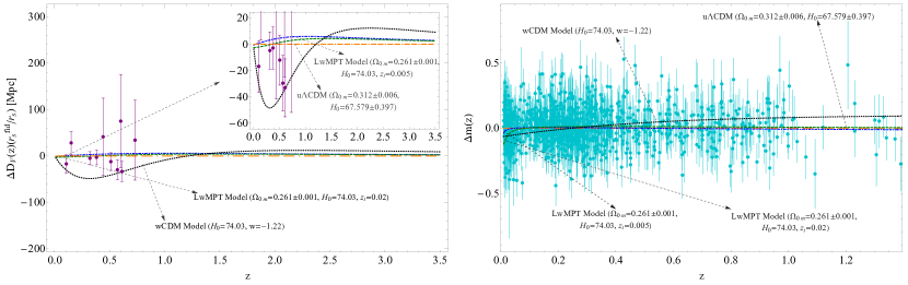
Figure 5: Left panel: BAO data residuals $\Delta D_{V}\times\frac{r_{s}^{fid}}{r_{s}}$ from the best fit u$\Lambda$CDM (orange dashed line) superimposed with the best fit residual curves corresponding to $wCDM$ (dotted black line), $LwMPT$ with $z_{t}=0.005$ (blue dot dashed line) and $LwMPT$ with $z_{t}=0.02$ (green dashed line). Notice the difficulty of smooth $H(z)$ deformation of $wCDM$ to fit the data due to the constraint imposed by the local measurements of Hubble constant. Right panel: The Pantheon SnIa distance modulus residuals $\Delta m$ from the best fit u$\Lambda$CDM. The predicted distance modulus residual curves for $wCDM$ (black dashed line), the $LwMPT$ ($z_{t}=0.005$) (blue dot dashed line) and the $LwMPT$ ($z_{t}=0.02$) (green dashed line) are also shown.

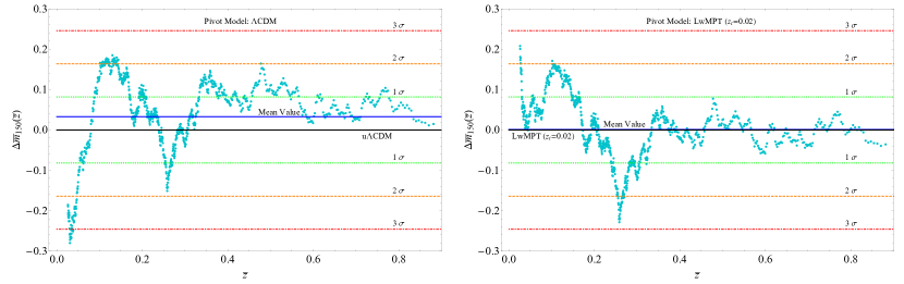
Figure 6: Left panel: The 150 point moving average of the Pantheon SnIa standardized residual absolute magnitudes with respect to the best fit $\Lambda$CDM ($\Delta{\bar{m}}_{150}(\bar{z})$ of eqs (16-17)). Notice the sharp and peculiar drop at $z\lesssim 0.1$ (unlikely at more than $3\sigma$ level). Right panel: The 150 point moving average of the Pantheon SnIa standardized residuals with respect to the best fit $LwMPT$ ($z_{t}=0.02$). The sharp drop shown in the left panel has disappeared while the mean and the standard deviation of the moving average points have dropped significantly indicating that the $LwMPT$ is a more natural pivot model than Planck18/$\Lambda$CDM.

Table 1: The values of the $LwMPT$ model best fit parameters $\Omega_{0m}$, $w_{<}$ ($z<z_{t}$) and $w_{>}$ ($z>z_{t}$) corresponding to different indicative values of the transition redshift $z_{t}$, along with each case’s $\Delta\chi^{2}$ with respect to u$\Lambda$CDM. In parenthesis we show the analytically predicted values of $w_{<}$ which were obtained from eq. (8) (i.e. assuming $w_{>}=-1$ and imposing the constraint $h(z=0)=h_{local}$ on the $LwMPT$ ansatz (4)). Notice that the best fit values of $\Omega_{0m}$ are consistent with the CMB spectrum requirement of $\omega_{m}=0.143$ in view of the constraint $h(z=0)=h_{local}$ imposed in all cases.

$z_{t}$	$\Delta\chi^{2}$	$\Omega_{0m}$	$w_{<}$ ($z<z_{t}$)	$w_{>}$ ($z>z_{t}$)
0.005	-1.9	0.2609	$-18.44\,(-18.4)$	-1.005
0.01	0.8	0.2608	$-9.93\,(-9.7)$	-1.001
0.02	9.7	0.2607	$-5.28\,(-5.3)$	-1.011
0.04	23.1	0.2606	$-2.93\,(-3.2)$	-1.037
0.05	27.6	0.2607	$-2.48\,(-2.8)$	-1.049
0.06	31.3	0.2607	$-2.19\,(-2.5)$	-1.059
0.08	37.9	0.2608	$-1.81\,(-2.1)$	-1.085
0.1	43.3	0.2611	$-1.58\,(-1.9)$	-1.115
0.2	50.1	0.2622	$-1.22\,(-1.4)$	-1.230

The forms of the comoving Hubble parameter $H(z)/(1+z)$ for two $LwMPT$ models with $z_{t}<0.1$, the best fit $wCDM$ and u$\Lambda$CDM are shown in Fig. 4. This figure demonstrates the efficiency of $LwMPT$ in mimicking the best fit u$\Lambda$CDM model (which is almost identical with Planck18/$\Lambda$CDM) while at the same time addressing the Hubble tension by reaching $h(z=0)=h_{local}$ in a continuous manner. On the other hand the smoother approach of $wCDM$ is much less efficient in mimicking Planck18/$\Lambda$CDM and the price it pays for this inability is a much worse quality of fit compared to $LwMPT$ as shown in Fig. 3.

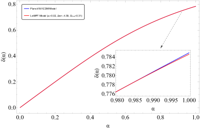
Figure 7: The growth factors $\delta(\alpha)$ of the linear perturbations, for both the $LwMPT$, with $z_{t}=0.02$ and $\Delta w=-4.39$ (red line), and Planck18/$\Lambda$CDM (blue line) models. Clearly, the effect of the $w$ transition on the growth factor is negligible at it occurs at $a_{t}\simeq 0.98$.

The difficulty of the smooth $H(z)$ deformation models that address the Hubble tension in fitting the BAO and SnIa data is also demonstrated in Fig. 5 where we show the BAO and SnIa data (residuals from the best fit u$\Lambda$CDM) along with the best fit residuals for the $wCDM$ and $LwMPT$ models.

The right panel of Fig. 5 indicates that the $LwMPT$ model with $z_{t}=0.02$ which can resolve the Hubble tension, closely mimics the apparent magnitudes of u$\Lambda$CDM for $z>z_{t}$ but for $z<z_{t}$ it predicts a small reduction of the residual apparent magnitudes. The question therefore to address is the following: Is there a hint for such a statistically significant reduction of the measured absolute magnitudes in redshifts close to the transition redshift $z_{t}\simeq 0.02$? Interestingly, this is indeed the case!

The left panel of Fig. 6 shows the $N=150$ point moving average of the standardized residual absolute magnitudes with respect to the best fit $\Lambda$CDM model. The $\Lambda$CDM standardized residual apparent magnitudes are defined as

$$\Delta\bar{m}(z_{i})\equiv\frac{m_{obs}(z_{i})-m_{th\Lambda CDM}(z_{i},M_{bf},\Omega_{0mbf})}{\sigma_{i-tot}}$$ (15)

where $\sigma_{i-tot}$ is the total error (statistical+systematic), $M_{bf}=-19.23$ and $\Omega_{0mbf}=0.30$ are the best fit parameter values of $\Lambda$CDM in the context of the Pantheon data and $m_{th\Lambda CDM}$ are the corresponding theoretically predicted apparent magnitudes. The $N$ point moving average corresponding to the residual standardized datapoint point $j$ ($j\in[1,1048-N]$) is defined as

$$\Delta{\bar{m}}_{N}^{j}({\bar{z}})\equiv\frac{1}{N}\sum_{i=j}^{j+N}\Delta{\bar{m}}(z_{i})$$ (16)

and the corresponding redshift is

$${\bar{z}}_{N}^{j}\equiv\frac{1}{N}\sum_{i=j}^{j+N}z_{i}$$ (17)

For $N=150$ the left panel of Fig. 6 shows the form of $\Delta{\bar{m}}_{N}({\bar{z}})$. Since the points are standardized and ignoring their correlations, we expect that the $1\sigma$ region will approximately correspond to $\sigma\simeq 1/\sqrt{N}\simeq 0.08$ which is also indicated in Fig. 6 up to the $3\sigma$ level. Interesting features of the binned Pantheon data have been identified in previous studies Kazantzidis et al. (2020); Kazantzidis and Perivolaropoulos (2020). Related to such features is a clear abrupt drop of the moving average of the standardized residuals from the $+2\sigma$ region to the $-3\sigma$ region and beyond clearly seen in the left panel of Fig. 6. The deepest part of this drop is at a redshift of about $0.02$. This is precisely the type of signature anticipated in the context of the $LwMPT$ model. Once we consider the residuals with respect not to the best fit $\Lambda$CDM but to the best fit $LwMPT$ model with $z_{t}=0.02$, this peculiar feature disappears (Fig. 6 right panel). In addition, the standard deviation of the points of the moving average of residuals decreases by about $20\%$ (from $0.1$ to $0.8$) while their mean value shown in Fig. 6 drops sharply from $0.03$ to $0.001$. This is also a hint that the best fit $LwMPT$ with $z_{t}=0.02$ is a more natural pivot model than the best fit $\Lambda$CDM. This observation supports the consideration of a combined $w-M$ transition for the resolution of the Hubble tension instead of using simply an $M$ transition.

In contrast to smooth $H(z)$ deformations that in general tend to worsen the growth tension by increasing the growth rate of cosmological perturbations at early times Alestas and Perivolaropoulos (2021) the proposed ultra-late $w$ transitions have negligible effect on the growth rate of cosmological perturbations. At $z_{t}=0.02$ most structures have already gone nonlinear during the $w=-1$ era and have decoupled from the effects of the background expansion. Even those fluctuations that are still linear do not have the time to respond to the change of $w$ since it occurs at very low $z$ ($z\simeq 0.02$). In addition, the emerging strongly phantom background could only lead to a suppression of the growth due the super accelerating expansion which prevents the growth of perturbations. We demonstrate this minor suppressing effect on the growth in Fig. 7, where we have solved numerically the equation for the growth of linear perturbations for the $LwMPT$ model for $z_{t}=0.02$ and for the required $\Delta w=-4.39$ showing that the effect on the growth factor is negligible compared to the Planck18/$\Lambda$CDM growth factor. If the effect of a possible gravitational transition inducing the change of $M$ were to be taken into account, the decrease of the growth factor may be shown to be large enough to resolve also the growth tension Marra and Perivolaropoulos (2021).

In order to identify the magnitude of the required $M$ transition we evaluate the best fit value of the absolute magnitude $M_{bf}(z_{t})$ for $z_{t}\it[0.01,0.15]$ (Fig. 8). Notice that $\Delta M\equiv M_{C}-M_{bf}$ is maximum at $z_{t}=0.01$ and approaches the $1\sigma$ distance from $M_{C}$ at $z_{t}>0.15$. For such high values of $z_{t}$ however the BAO data are poorly fit and the value of $\chi^{2}$ increases to the level of $wCDM$. The type of the required $M$ transition for $z_{t}=0.02$ is shown in the left panel of Fig. 9 where we also show the absolute magnitudes of the binned Pantheon datapoints obtained from eq. (13) by solving with respect to $M$ for each datapoint and using the best fit form of $D_{L}(z)$ for $z_{t}=0.02$. Clearly, the derived absolute magnitudes are not consistent with the Cepheid calibrated value of $M_{C}$ but in the context of an $M$ transition with $\Delta M\simeq-0.1$ the inconsistency disappears. The right panel of Fig. 9 shows the required evolution of an effective Newton’s constant that is required to produce the $M$ transition obtained under the assumption that the SnIa absolute luminosity is proportional to the Chandrasekhar mass which varies as $L\sim G_{\rm eff}^{b}$ with $b=-3/2$. This assumption leads to the variation of the SnIa absolute magnitude $M$ with $\mu\equiv\frac{G_{\rm eff}}{G_{\rm N}}$ ($G_{\rm N}$ is the locally measured Newton’s constant) as Amendola et al. (1999); Gaztanaga et al. (2002); Kazantzidis and Perivolaropoulos (2019)

$$\Delta M=\frac{15}{4}\,log_{10}\,\left(\mu\right)$$ (18)

which implies that for $\Delta M\simeq-0.1$ we have a $6\%$ reduction of $\mu$.

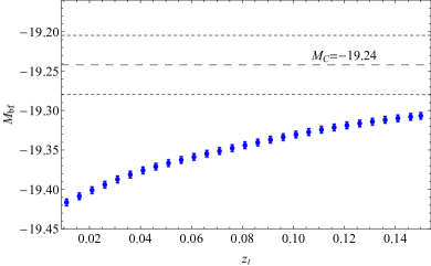
Figure 8: The best fit absolute magnitude $M_{bf}$ (blue points) for various transitions $z_{t}$ for the $LwMPT$ model. The dashed line corresponds to the $M_{C}$ value indicated by Refs. Camarena and Marra (2020, 2021), while the dot dashed lines correspond its $1\sigma$ error. Notice that if $M_{C}$ is considered to be constant, the majority of the best fit values of $M_{bf}$ are more than $2\sigma$ away from the $M_{C}$ value. This difference reduces as $z_{t}$ increases.

Notice that if the SnIa data analysis assumes a fixed value of $M=M_{C}$ then the existing $m(z_{i})$ data lead to a value of $H_{0}=74km/(sec\cdot Mpc)$ while if the transitions (1) and (2) are assumed with $z_{t}=0.02$, $\Delta w=-4.3$ and $\Delta M=-0.1$ then the data analysis would lead to a value $H_{0}=67.5km/(sec\cdot Mpc)$ (consistent with CMB-BAO calibration) while the true value of $H_{0}$ would be $H_{0}=74km/(sec\cdot Mpc)$ due to the $H_{0}$ prior imposed on the $w$ transition $\Delta w$.

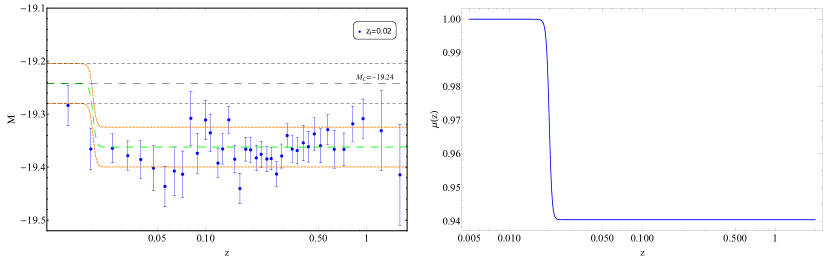
Figure 9: Left panel: The absolute magnitude $M$ as a function of redshift $z$. The straight dashed line corresponds to the fixed $M_{C}$ value Camarena and Marra (2020, 2021) from local Cepheid calibrators of SnIa while the dot dashed lines correspond to its $1\sigma$ error. Clearly Pantheon binned absolute magnitudes $M_{i}$ (blue points) corresponding to the best fit $LwMPT$ model $(z_{t}=0.02)$ are approximately $2\sigma$ away from $M_{C}$. However, in the context of an abrupt transition of $M$ with $\Delta M\simeq-0.1$ at $z_{t}=0.02$, the inconsistency disappears. Right panel: The form of $\mu=G_{\rm eff}/G_{\rm N}$ required to induce he $M$ transition shown on the left panel. Clearly, for $z>0.02$ $G_{\rm eff}<1$ hinting towards weaker gravity Gannouji et al. (2018, 2020); Amendola et al. (2018) as indicated by other studies discussing the growth tension Hildebrandt et al. (2017); Joudaki et al. (2018); Abbott et al. (2018); Kazantzidis and Perivolaropoulos (2019); Skara and Perivolaropoulos (2020); Kazantzidis et al. (2020).

IV Conclusion-Discussion-Outlook

We have demonstrated using both an analytical approach and a fit to cosmological data that a Late dark energy equation of state $w$ Phantom Transition ($LwMPT$) from $w_{>}=-1$ ($z>z_{t}$) to $w_{<}<-1$ ($z<z_{t}$) at transition redshift $z_{t}\in[0.01,0.1]$ can lead to a resolution of the Hubble tension in a more efficient manner than smooth deformations of the Hubble tension and other types of late time transitions (the Hubble expansion rate transition). The required type of transition is a phantom transition with $w_{<}(z_{t})\in[-2,-10]$ for $z<z_{t}$. The moving average statistic of the standardized residual Pantheon absolute magnitude SnIa data indicates the presence of a peculiar feature at $z<0.1$ which is consistent with the anticipated signatures of the $LwMPT$ model. Such a transition leads in general to a best fit value of the SnIa absolute magnitude that is not consistent with the value implied by local Cepheid calibrators of SnIa Camarena and Marra (2021). Therefore late time transitions can only constitute successful resolutions of the Hubble tension if they are accompanied by a transition of the SnIa absolute magnitude due to evolving fundamental constants. We have shown that a transition of the effective gravitational constant to a value lower by about $6\%$ is sufficient to induce the required $\Delta M$ transition. This weakening of gravity may also justify the observed reduced growth of perturbations which is supported by Weak Lensing Hildebrandt et al. (2017); Joudaki et al. (2018); Abbott et al. (2018) and Redshift Space Distortion data Kazantzidis and Perivolaropoulos (2019); Skara and Perivolaropoulos (2020); Kazantzidis et al. (2020) (growth tension). Therefore, this model simultaneously addresses both the Hubble and the growth tensions.

Another basic advantage of such a late time model that can fully resolve the Hubble tension is that it can fit the local distance data (BAO and SnIa) in a very effective manner. This is due to the fact that by construction it has the same quality of fit to the BAO, SnIa and CMB data as Planck18/$\Lambda$CDM, in contrast to the usual late time smooth deformations of $H(z)$.

Moreover, there is a physical theoretical basis of the model since it can be realized in the context of modified gravity theory with a rapid gravitational transition. The rapid nature of the transition is a generic feature and can be made consistent with solar system tests with no need for screening as in other modified theories. Such models include the following:

• The most natural model that can induce a $LwMPT$ involves a non-minimally coupled phantom scalar field initially frozen at $\phi=\phi_{0}$ due to cosmic friction close to the zero point of its potential which could be assumed to be of the form $V(\phi)=s\;\phi^{n}$. Such a field would initially have a dark energy equation of state $w=-1$ mimicking a cosmological constant. Once Hubble friction becomes smaller than the field dynamical (mass) scale, the field becomes free to roll up its potential (phantom fields move up their potential in contrast to quintessence fields Perivolaropoulos (2005a); Nesseris and Perivolaropoulos (2007)) and develops a rapidly changing equation of state parameter $w<-1$ and shifted $G_{\rm eff}$. Thus the universe enters a ghost instability phase which will end in a Big Rip singularity in less than a Hubble time. Such a scenario for the simple (but also generic) case of linear potential ($n=1$) has been investigated in Ref. Perivolaropoulos (2005a). For a general phantom potential we anticipate a redshift dependence of the equation of state $w_{<}=w_{<}(z)$ after the transition ($z<z_{t}$). In fact the phantom field potential could be reconstructed by demanding a form of $w_{<}(z)$ that further optimizes the quality of fit to the low $z$ data or by simply demanding that $w_{<}$ is constant.

• A scalar-tensor modified gravity theory field initially frozen due to Hubble friction, mimicking general relativity and a cosmological constant. Once Hubble friction becomes smaller than the field mass scale, the field becomes free to roll down its potential inducing deviations from general relativity on cosmological scales and a phantom departure from the cosmological constant. Note that scalar tensor theories can induce phantom behavior without instabilities in contrast to a simple minimally coupled scalar field Perivolaropoulos (2005b).

The detailed investigation of the above described dynamical scalar field evolution that can reproduce the $LwMPT$ is an interesting extension of the present analysis.

If the phantom $LwMPT$ is realized in Nature it would imply the existence of a rapidly approaching Big Rip singularity Caldwell et al. (2003); Nesseris and Perivolaropoulos (2004) which may be avoided due to quantum effects Elizalde et al. (2004). Given the value of $w_{<}$ which emerges at approximately the present time $t_{0}$, it is straightforward to calculate the time $t_{*}$ of the Big Rip singularity assuming that $w=w_{<}<-1$ at the present time $t_{0}$. The result is Nesseris and Perivolaropoulos (2004)

$$\frac{t_{*}}{t_{0}}=\frac{w_{<}}{1+w_{<}}$$ (19)

For example for $z_{t}=0.02$ we have $w_{<}\simeq-5$ which implies that the universe will end in a Big Rip singularity in less than $3.5$ billion years (for $t_{0}=13.8\times 10^{9}yrs$). This implies that there may be observational effects of such coming singularity on the largest bound systems like the Virgo cluster, the Coma Cluster or the Virgo supercluster. A detailed investigation of the observational effects on bound systems of the $LwMPT$ is an interesting extension of the present analysis.

The detailed comparison of the quality of fit of the $LwMPT$ (or similar) models with a variety of smooth $H(z)$ deformation models addressing the Hubble tension would also be a useful extension. The use of full CMB spectrum data and possibly other cosmological data sensitive to the dynamics of galaxies in clusters and superclusters could also be included.

The late time sudden deformation of the luminosity distance $D_{L}(z)$ induced through the $w$ transition helps to decrease the required magnitude of the $M$ transition from $\Delta M\simeq-0.2$ to $\Delta M\simeq-0.1$. In the absence of the $w$ transition the Hubble tension could still be resolved via an $M$ transition with $\Delta M\simeq-0.2$ and no deformation of $D_{L}(z)$. Even though this approach would be simpler it would require a larger amplitude of the $\Delta M$ transition at $z_{t}\simeq 0.01$ while it would not address the abrupt feature in the Pantheon data shown in Fig. 6. Nevertheless, the simplicity of such an approach in an attractive feature and thus this model deserves a detailed investigation by comparing its predictions with current and future data.

Numerical Analysis Files: The numerical files for the reproduction of the figures can be found here.

Appendix A Data Used in the Analysis

The covariance matrix which corresponds to the latest Planck18/$\Lambda$CDM CMB distance prior data (shift parameter $R$ and the acoustic scale $l_{a}$), for a flat universe has the following form Zhai and Wang (2019)

$$C_{ij}=10^{-8}\times\begin{pmatrix}1598.9554~{}~{}17112.007\\ 17112.007~{}~{}811208.45\\ \end{pmatrix}$$

where the corresponding Planck18/$\Lambda$CDM values for $R$ and $l_{a}$ are presented in Table LABEL:tab:CMBdat. Furthermore, we present the full dataset of the BAO and CC likelihoods used in the Mathematica analysis in Tables LABEL:tab:data-bao and LABEL:tab:data-cc respectively.

Table 2: The CMB Distance Prior data for a flat Universe used in our analysis.

Index	CMB Observable	CMB Value	Reference
1	$R$	$1.74963$	Zhai and Wang (2019)
2	$l_{a}$	$301.80845$	Zhai and Wang (2019)

Table 3: The BAO data that have been used in the analysis along with the corresponding references.

Index	$z$	$D_{A}/r_{s}$ (Mpc)	$D_{H}/r_{s}(km/sec\cdot Mpc)$	$D_{V}/r_{s}$ (Mpc)	Ref.
1	$0.106$	-	-	$2.98\pm 0.13$	Beutler et al. (2011)
2	$0.44$	-	-	$13.69\pm 5.82$	Blake et al. (2012)
3	$0.6$	-	-	$13.77\pm 3.11$	Blake et al. (2012)
4	$0.73$	-	-	$16.89\pm 5.28$	Blake et al. (2012)
5	$2.34$	$11.28\pm 0.65$	-	-	de Sainte Agathe et al. (2019)
6	$2.34$	-	$9.18\pm 0.28$	-	de Sainte Agathe et al. (2019)
7	$0.15$	-	-	$4.465\pm 0.168$	Ross et al. (2015)
8	$0.32$	-	-	$8.62\pm 0.15$	Anderson et al. (2014)
9	$0.57$	-	-	$13.7\pm 0.12$	Anderson et al. (2014)

Table 4: The Cosmic Chronometer data that have been used in the analysis.

Index	$z$	$H(z)(km/sec\cdot Mpc)$	Ref.
1	$0.09$	$69\pm 12$	Jimenez et al. (2003)
2	$0.17$	$83\pm 8$	Simon et al. (2005)
3	$0.179$	$75\pm 4$	Moresco et al. (2012)
4	$0.199$	$75\pm 5$	Moresco et al. (2012)
5	$0.27$	$77\pm 14$	Simon et al. (2005)
6	$0.352$	$83\pm 14$	Moresco et al. (2012)
7	$0.3802$	$83\pm 13.5$	Moresco et al. (2016)
8	$0.4$	$95\pm 17$	Simon et al. (2005)
9	$0.4004$	$77\pm 10.2$	Moresco et al. (2016)
10	$0.4247$	$87.1\pm 11.2$	Moresco et al. (2016)
11	$0.4497$	$92.8\pm 12.9$	Moresco et al. (2016)
12	$0.4783$	$80.9\pm 9$	Moresco et al. (2016)
13	$0.48$	$97\pm 62$	Stern et al. (2010)
14	$0.593$	$104\pm 13$	Moresco et al. (2012)
15	$0.68$	$92\pm 8$	Moresco et al. (2012)
16	$0.781$	$105\pm 12$	Moresco et al. (2012)
17	$0.875$	$125\pm 17$	Zhang et al. (2012)
18	$0.88$	$90\pm 40$	Stern et al. (2010)
19	$0.9$	$117\pm 23$	Simon et al. (2005)
20	$1.037$	$154\pm 20$	Moresco et al. (2012)
21	$1.3$	$168\pm 17$	Simon et al. (2005)
22	$1.363$	$160\pm 33.6$	Moresco (2015)
23	$1.43$	$177\pm 18$	Simon et al. (2005)
24	$1.53$	$140\pm 14$	Simon et al. (2005)
25	$1.75$	$202\pm 40$	Simon et al. (2005)
26	$1.965$	$186.5\pm 50.4$	Moresco (2015)
27	$0.35$	$82.7\pm 8.4$	Chuang and Wang (2013)
28	$0.44$	$82.6\pm 7.8$	Blake et al. (2012)
29	$0.57$	$96.8\pm 3.4$	Anderson et al. (2014)
30	$0.6$	$87.9\pm 6.1$	Blake et al. (2012)
31	$0.73$	$97.3\pm 7$	Blake et al. (2012)
32	$2.34$	$222\pm 7$	Delubac et al. (2015)
33	$0.07$	$69\pm 19.6$	Zhang et al. (2012)
34	$0.12$	$68.6\pm 26.2$	Zhang et al. (2012)
35	$0.2$	$72.9\pm 29.6$	Zhang et al. (2012)
36	$0.24$	$79.69\pm 2.65$	Gaztañaga et al. (2009)
37	$0.28$	$88.8\pm 36.6$	Zhang et al. (2012)
38	$0.43$	$86.45\pm 3.68$	Gaztañaga et al. (2009)
39	$0.57$	$92.4\pm 4.5$	Samushia et al. (2013)
40	$2.3$	$224\pm 8$	Busca et al. (2013)
41	$2.36$	$226\pm 8$	et al. (2014)

References

- Riess et al. (2019) Adam G. Riess, Stefano Casertano, Wenlong Yuan, Lucas M. Macri, and Dan Scolnic, “Large Magellanic Cloud Cepheid Standards Provide a 1% Foundation for the Determination of the Hubble Constant and Stronger Evidence for Physics beyond CDM,” Astrophys. J. 876, 85 (2019), arXiv:1903.07603 [astro-ph.CO] .
- Riess et al. (2018) Adam G. Riess et al., “Milky Way Cepheid Standards for Measuring Cosmic Distances and Application to Gaia DR2: Implications for the Hubble Constant,” Astrophys. J. 861, 126 (2018), arXiv:1804.10655 [astro-ph.CO] .
- Riess et al. (2016) Adam G. Riess et al., “A 2.4% Determination of the Local Value of the Hubble Constant,” Astrophys. J. 826, 56 (2016), arXiv:1604.01424 [astro-ph.CO] .
- Freedman et al. (2020) Wendy L. Freedman, Barry F. Madore, Taylor Hoyt, In Sung Jang, Rachael Beaton, Myung Gyoon Lee, Andrew Monson, Jill Neeley, and Jeffrey Rich, “Calibration of the Tip of the Red Giant Branch (TRGB),” (2020), 10.3847/1538-4357/ab7339, arXiv:2002.01550 [astro-ph.GA] .
- Freedman et al. (2019) Wendy L. Freedman et al., “The Carnegie-Chicago Hubble Program. VIII. An Independent Determination of the Hubble Constant Based on the Tip of the Red Giant Branch,” (2019), 10.3847/1538-4357/ab2f73, arXiv:1907.05922 [astro-ph.CO] .
- Pesce et al. (2020) D.W. Pesce et al., “The Megamaser Cosmology Project. XIII. Combined Hubble constant constraints,” Astrophys. J. Lett. 891, L1 (2020), arXiv:2001.09213 [astro-ph.CO] .
- Aghanim et al. (2020) N. Aghanim et al. (Planck), “Planck 2018 results. VI. Cosmological parameters,” Astron. Astrophys. 641, A6 (2020), arXiv:1807.06209 [astro-ph.CO] .
- Addison et al. (2018) G.E. Addison, D.J. Watts, C.L. Bennett, M. Halpern, G. Hinshaw, and J.L. Weiland, “Elucidating CDM: Impact of Baryon Acoustic Oscillation Measurements on the Hubble Constant Discrepancy,” Astrophys. J. 853, 119 (2018), arXiv:1707.06547 [astro-ph.CO] .
- Schöneberg et al. (2019) Nils Schöneberg, Julien Lesgourgues, and Deanna C. Hooper, “The BAO+BBN take on the Hubble tension,” JCAP 10, 029 (2019), arXiv:1907.11594 [astro-ph.CO] .
- Birrer et al. (2019) S. Birrer et al., “H0LiCOW - IX. Cosmographic analysis of the doubly imaged quasar SDSS 1206+4332 and a new measurement of the Hubble constant,” Mon. Not. Roy. Astron. Soc. 484, 4726 (2019), arXiv:1809.01274 [astro-ph.CO] .
- Shajib et al. (2020) A.J. Shajib et al. (DES), “STRIDES: a 3.9 per cent measurement of the Hubble constant from the strong lens system DES J04085354,” Mon. Not. Roy. Astron. Soc. 494, 6072–6102 (2020), arXiv:1910.06306 [astro-ph.CO] .
- Abbott et al. (2019) B.P. Abbott et al. (LIGO Scientific, Virgo), “A gravitational-wave measurement of the Hubble constant following the second observing run of Advanced LIGO and Virgo,” (2019), arXiv:1908.06060 [astro-ph.CO] .
- Soares-Santos et al. (2019) M. Soares-Santos et al. (DES, LIGO Scientific, Virgo), “First Measurement of the Hubble Constant from a Dark Standard Siren using the Dark Energy Survey Galaxies and the LIGO/Virgo Binary–Black-hole Merger GW170814,” Astrophys. J. Lett. 876, L7 (2019), arXiv:1901.01540 [astro-ph.CO] .
- Knox and Millea (2020) Lloyd Knox and Marius Millea, “Hubble constant hunter’s guide,” Phys. Rev. D 101, 043533 (2020), arXiv:1908.03663 [astro-ph.CO] .
- Mörtsell and Dhawan (2018) Edvard Mörtsell and Suhail Dhawan, “Does the Hubble constant tension call for new physics?” JCAP 09, 025 (2018), arXiv:1801.07260 [astro-ph.CO] .
- Efstathiou (2020) G. Efstathiou, “A Lockdown Perspective on the Hubble Tension (with comments from the SH0ES team),” (2020), arXiv:2007.10716 [astro-ph.CO] .
- Kazantzidis and Perivolaropoulos (2020) L. Kazantzidis and L. Perivolaropoulos, “Hints of a Local Matter Underdensity or Modified Gravity in the Low Pantheon data,” Phys. Rev. D 102, 023520 (2020), arXiv:2004.02155 [astro-ph.CO] .
- Kazantzidis et al. (2020) L. Kazantzidis, H. Koo, S. Nesseris, L. Perivolaropoulos, and A. Shafieloo, “Hints for possible low redshift oscillation around the best fit CDM model in the expansion history of the universe,” (2020), 10.1093/mnras/staa3866, arXiv:2010.03491 [astro-ph.CO] .
- Sapone et al. (2020) Domenico Sapone, Savvas Nesseris, and Carlos A.P. Bengaly, “Is there any measurable redshift dependence on the SN Ia absolute magnitude?” (2020), arXiv:2006.05461 [astro-ph.CO] .
- Soltis et al. (2020) John Soltis, Stefano Casertano, and Adam G. Riess, “The Parallax of Omega Centauri Measured from Gaia EDR3 and a Direct, Geometric Calibration of the Tip of the Red Giant Branch and the Hubble Constant,” (2020), arXiv:2012.09196 [astro-ph.GA] .
- Riess et al. (2020) Adam G. Riess, Stefano Casertano, Wenlong Yuan, J. Bradley Bowers, Lucas Macri, Joel C. Zinn, and Dan Scolnic, “Cosmic Distances Calibrated to 1% Precision with Gaia EDR3 Parallaxes and Hubble Space Telescope Photometry of 75 Milky Way Cepheids Confirm Tension with LambdaCDM,” (2020), arXiv:2012.08534 [astro-ph.CO] .
- Blinov et al. (2019) Nikita Blinov, Kevin James Kelly, Gordan Z Krnjaic, and Samuel D McDermott, “Constraining the Self-Interacting Neutrino Interpretation of the Hubble Tension,” Phys. Rev. Lett. 123, 191102 (2019), arXiv:1905.02727 [astro-ph.CO] .
- Poulin et al. (2019) Vivian Poulin, Tristan L. Smith, Tanvi Karwal, and Marc Kamionkowski, “Early Dark Energy Can Resolve The Hubble Tension,” Phys. Rev. Lett. 122, 221301 (2019), arXiv:1811.04083 [astro-ph.CO] .
- Sakstein and Trodden (2020) Jeremy Sakstein and Mark Trodden, “Early Dark Energy from Massive Neutrinos as a Natural Resolution of the Hubble Tension,” Phys. Rev. Lett. 124, 161301 (2020), arXiv:1911.11760 [astro-ph.CO] .
- Agrawal et al. (2019) Prateek Agrawal, Francis-Yan Cyr-Racine, David Pinner, and Lisa Randall, “Rock ’n’ Roll Solutions to the Hubble Tension,” (2019), arXiv:1904.01016 [astro-ph.CO] .
- Lin et al. (2019) Meng-Xiang Lin, Giampaolo Benevento, Wayne Hu, and Marco Raveri, “Acoustic Dark Energy: Potential Conversion of the Hubble Tension,” Phys. Rev. D 100, 063542 (2019), arXiv:1905.12618 [astro-ph.CO] .
- Braglia et al. (2020) Matteo Braglia, William T. Emond, Fabio Finelli, A. Emir Gumrukcuoglu, and Kazuya Koyama, “Unified framework for Early Dark Energy from -attractors,” (2020), arXiv:2005.14053 [astro-ph.CO] .
- Niedermann and Sloth (2020) Florian Niedermann and Martin S. Sloth, “Resolving the Hubble Tension with New Early Dark Energy,” Phys. Rev. D 102, 063527 (2020), arXiv:2006.06686 [astro-ph.CO] .
- Smith et al. (2020a) Tristan L. Smith, Vivian Poulin, José Luis Bernal, Kimberly K. Boddy, Marc Kamionkowski, and Riccardo Murgia, “Early dark energy is not excluded by current large-scale structure data,” (2020a), arXiv:2009.10740 [astro-ph.CO] .
- Benisty (2019) David Benisty, “Decaying coupled Fermions to curvature and the tension,” (2019), arXiv:1912.11124 [gr-qc] .
- Ballardini et al. (2020) Mario Ballardini, Matteo Braglia, Fabio Finelli, Daniela Paoletti, Alexei A. Starobinsky, and Caterina Umiltà, “Scalar-tensor theories of gravity, neutrino physics, and the tension,” JCAP 10, 044 (2020), arXiv:2004.14349 [astro-ph.CO] .
- D’Amico et al. (2020) Guido D’Amico, Leonardo Senatore, Pierre Zhang, and Henry Zheng, “The Hubble Tension in Light of the Full-Shape Analysis of Large-Scale Structure Data,” (2020), arXiv:2006.12420 [astro-ph.CO] .
- Haridasu et al. (2020) Balakrishna S. Haridasu, Matteo Viel, and Nicola Vittorio, “Sources of -tensions in dark energy scenarios,” (2020), arXiv:2012.10324 [astro-ph.CO] .
- Krishnan et al. (2020a) C. Krishnan, Eoin Ó. Colgáin, Ruchika, Anjan A. Sen, M.M. Sheikh-Jabbari, and Tao Yang, “Is there an early Universe solution to Hubble tension?” Phys. Rev. D 102, 103525 (2020a), arXiv:2002.06044 [astro-ph.CO] .
- Hildebrandt et al. (2017) H. Hildebrandt et al., “KiDS-450: Cosmological parameter constraints from tomographic weak gravitational lensing,” Mon. Not. Roy. Astron. Soc. 465, 1454 (2017), arXiv:1606.05338 [astro-ph.CO] .
- Joudaki et al. (2018) Shahab Joudaki et al., “KiDS-450 + 2dFLenS: Cosmological parameter constraints from weak gravitational lensing tomography and overlapping redshift-space galaxy clustering,” Mon. Not. Roy. Astron. Soc. 474, 4894–4924 (2018), arXiv:1707.06627 [astro-ph.CO] .
- Köhlinger et al. (2017) F. Köhlinger et al., “KiDS-450: The tomographic weak lensing power spectrum and constraints on cosmological parameters,” Mon. Not. Roy. Astron. Soc. 471, 4412–4435 (2017), arXiv:1706.02892 [astro-ph.CO] .
- Abbott et al. (2018) T.M.C. Abbott et al. (DES), “Dark Energy Survey year 1 results: Cosmological constraints from galaxy clustering and weak lensing,” Phys. Rev. D 98, 043526 (2018), arXiv:1708.01530 [astro-ph.CO] .
- Macaulay et al. (2013) Edward Macaulay, Ingunn Kathrine Wehus, and Hans Kristian Eriksen, “Lower Growth Rate from Recent Redshift Space Distortion Measurements than Expected from Planck,” Phys. Rev. Lett. 111, 161301 (2013), arXiv:1303.6583 [astro-ph.CO] .
- Kazantzidis and Perivolaropoulos (2018) Lavrentios Kazantzidis and Leandros Perivolaropoulos, “Evolution of the tension with the Planck15/CDM determination and implications for modified gravity theories,” Phys. Rev. D 97, 103503 (2018), arXiv:1803.01337 [astro-ph.CO] .
- Nesseris et al. (2017) Savvas Nesseris, George Pantazis, and Leandros Perivolaropoulos, “Tension and constraints on modified gravity parametrizations of from growth rate and Planck data,” Phys. Rev. D 96, 023542 (2017), arXiv:1703.10538 [astro-ph.CO] .
- Skara and Perivolaropoulos (2020) F. Skara and L. Perivolaropoulos, “Tension of the statistic and redshift space distortion data with the Planck - model and implications for weakening gravity,” Phys. Rev. D 101, 063521 (2020), arXiv:1911.10609 [astro-ph.CO] .
- Kazantzidis and Perivolaropoulos (2019) Lavrentios Kazantzidis and Leandros Perivolaropoulos, “Is gravity getting weaker at low z? Observational evidence and theoretical implications,” (2019), arXiv:1907.03176 [astro-ph.CO] .
- Kazantzidis et al. (2019) L. Kazantzidis, L. Perivolaropoulos, and F. Skara, “Constraining power of cosmological observables: blind redshift spots and optimal ranges,” Phys. Rev. D 99, 063537 (2019), arXiv:1812.05356 [astro-ph.CO] .
- Di Valentino et al. (2021) Eleonora Di Valentino, Olga Mena, Supriya Pan, Luca Visinelli, Weiqiang Yang, Alessandro Melchiorri, David F. Mota, Adam G. Riess, and Joseph Silk, “In the Realm of the Hubble tension a Review of Solutions,” (2021), arXiv:2103.01183 [astro-ph.CO] .
- Alestas et al. (2020) G. Alestas, L. Kazantzidis, and L. Perivolaropoulos, “ tension, phantom dark energy, and cosmological parameter degeneracies,” Phys. Rev. D 101, 123516 (2020), arXiv:2004.08363 [astro-ph.CO] .
- Di Valentino et al. (2016) Eleonora Di Valentino, Alessandro Melchiorri, and Joseph Silk, “Reconciling Planck with the local value of in extended parameter space,” Phys. Lett. B 761, 242–246 (2016), arXiv:1606.00634 [astro-ph.CO] .
- Smith et al. (2020b) Tristan L. Smith, Vivian Poulin, and Mustafa A. Amin, “Oscillating scalar fields and the Hubble tension: a resolution with novel signatures,” Phys. Rev. D 101, 063523 (2020b), arXiv:1908.06995 [astro-ph.CO] .
- Vagnozzi (2020) Sunny Vagnozzi, “New physics in light of the tension: An alternative view,” Phys. Rev. D 102, 023518 (2020), arXiv:1907.07569 [astro-ph.CO] .
- Li and Shafieloo (2019) Xiaolei Li and Arman Shafieloo, “A Simple Phenomenological Emergent Dark Energy Model can Resolve the Hubble Tension,” Astrophys. J. Lett. 883, L3 (2019), arXiv:1906.08275 [astro-ph.CO] .
- Di Valentino et al. (2020) Eleonora Di Valentino, Ankan Mukherjee, and Anjan A. Sen, “Dark Energy with Phantom Crossing and the tension,” (2020), arXiv:2005.12587 [astro-ph.CO] .
- Krishnan et al. (2020b) Chethan Krishnan, Eoin O. Colgain, M.M. Sheikh-Jabbari, and Tao Yang, “Running Hubble Tension and a H0 Diagnostic,” (2020b), arXiv:2011.02858 [astro-ph.CO] .
- Mortonson et al. (2009) Michael J. Mortonson, Wayne Hu, and Dragan Huterer, “Hiding dark energy transitions at low redshift,” Phys. Rev. D 80, 067301 (2009), arXiv:0908.1408 [astro-ph.CO] .
- Benevento et al. (2020) Giampaolo Benevento, Wayne Hu, and Marco Raveri, “Can Late Dark Energy Transitions Raise the Hubble constant?” Phys. Rev. D 101, 103517 (2020), arXiv:2002.11707 [astro-ph.CO] .
- Dhawan et al. (2020) S. Dhawan, D. Brout, D. Scolnic, A. Goobar, A.G. Riess, and V. Miranda, “Cosmological Model Insensitivity of Local from the Cepheid Distance Ladder,” Astrophys. J. 894, 54 (2020), arXiv:2001.09260 [astro-ph.CO] .
- Keeley et al. (2019) Ryan E. Keeley, Shahab Joudaki, Manoj Kaplinghat, and David Kirkby, “Implications of a transition in the dark energy equation of state for the and tensions,” JCAP 12, 035 (2019), arXiv:1905.10198 [astro-ph.CO] .
- Bassett et al. (2002) Bruce A. Bassett, Martin Kunz, Joseph Silk, and Carlo Ungarelli, “A Late time transition in the cosmic dark energy?” Mon. Not. Roy. Astron. Soc. 336, 1217–1222 (2002), arXiv:astro-ph/0203383 .
- Camarena and Marra (2021) David Camarena and Valerio Marra, “Hockey-stick dark energy is not a solution to the crisis,” (2021), arXiv:2101.08641 [astro-ph.CO] .
- Camarena and Marra (2020) David Camarena and Valerio Marra, “Local determination of the Hubble constant and the deceleration parameter,” Phys. Rev. Res. 2, 013028 (2020), arXiv:1906.11814 [astro-ph.CO] .
- Scolnic et al. (2018) D.M. Scolnic et al., “The Complete Light-curve Sample of Spectroscopically Confirmed SNe Ia from Pan-STARRS1 and Cosmological Constraints from the Combined Pantheon Sample,” Astrophys. J. 859, 101 (2018), arXiv:1710.00845 [astro-ph.CO] .
- Elgaroy and Multamaki (2007) Oystein Elgaroy and Tuomas Multamaki, “On using the CMB shift parameter in tests of models of dark energy,” Astron. Astrophys. 471, 65 (2007), arXiv:astro-ph/0702343 .
- Zhai and Wang (2019) Zhongxu Zhai and Yun Wang, “Robust and model-independent cosmological constraints from distance measurements,” JCAP 07, 005 (2019), arXiv:1811.07425 [astro-ph.CO] .
- Arjona et al. (2019) Rubén Arjona, Wilmar Cardona, and Savvas Nesseris, “Unraveling the effective fluid approach for models in the subhorizon approximation,” Phys. Rev. D 99, 043516 (2019), arXiv:1811.02469 [astro-ph.CO] .
- Alestas and Perivolaropoulos (2021) G. Alestas and L. Perivolaropoulos, “Late time approaches to the Hubble tension deforming , worsen the growth tension,” (2021), arXiv:2103.04045 [astro-ph.CO] .
- Marra and Perivolaropoulos (2021) Valerio Marra and Leandros Perivolaropoulos, “A rapid transition of at as a solution of the Hubble and growth tensions,” (2021), arXiv:2102.06012 [astro-ph.CO] .
- Wright and Li (2018) Bill S. Wright and Baojiu Li, “Type Ia supernovae, standardizable candles, and gravity,” Phys. Rev. D 97, 083505 (2018), arXiv:1710.07018 [astro-ph.CO] .
- Amendola et al. (1999) Luca Amendola, Pier Stefano Corasaniti, and Franco Occhionero, “Time variability of the gravitational constant and type Ia supernovae,” (1999), arXiv:astro-ph/9907222 .
- Gaztanaga et al. (2002) E. Gaztanaga, E. Garcia-Berro, J. Isern, E. Bravo, and I. Dominguez, “Bounds on the possible evolution of the gravitational constant from cosmological type Ia supernovae,” Phys. Rev. D 65, 023506 (2002), arXiv:astro-ph/0109299 .
- Gannouji et al. (2018) Radouane Gannouji, Lavrentios Kazantzidis, Leandros Perivolaropoulos, and David Polarski, “Consistency of modified gravity with a decreasing in a CDM background,” Phys. Rev. D 98, 104044 (2018), arXiv:1809.07034 [gr-qc] .
- Gannouji et al. (2020) Radouane Gannouji, Leandros Perivolaropoulos, David Polarski, and Foteini Skara, “Weak gravity on a CDM background,” (2020), arXiv:2011.01517 [gr-qc] .
- Amendola et al. (2018) Luca Amendola, Martin Kunz, Ippocratis D. Saltas, and Ignacy Sawicki, “Fate of Large-Scale Structure in Modified Gravity After GW170817 and GRB170817A,” Phys. Rev. Lett. 120, 131101 (2018), arXiv:1711.04825 [astro-ph.CO] .
- Perivolaropoulos (2005a) Leandros Perivolaropoulos, “Constraints on linear negative potentials in quintessence and phantom models from recent supernova data,” Phys. Rev. D 71, 063503 (2005a), arXiv:astro-ph/0412308 .
- Nesseris and Perivolaropoulos (2007) S. Nesseris and Leandros Perivolaropoulos, “Crossing the Phantom Divide: Theoretical Implications and Observational Status,” JCAP 01, 018 (2007), arXiv:astro-ph/0610092 .
- Perivolaropoulos (2005b) Leandros Perivolaropoulos, “Crossing the phantom divide barrier with scalar tensor theories,” JCAP 10, 001 (2005b), arXiv:astro-ph/0504582 .
- Caldwell et al. (2003) Robert R. Caldwell, Marc Kamionkowski, and Nevin N. Weinberg, “Phantom energy and cosmic doomsday,” Phys. Rev. Lett. 91, 071301 (2003), arXiv:astro-ph/0302506 .
- Nesseris and Perivolaropoulos (2004) S. Nesseris and Leandros Perivolaropoulos, “The Fate of bound systems in phantom and quintessence cosmologies,” Phys. Rev. D 70, 123529 (2004), arXiv:astro-ph/0410309 .
- Elizalde et al. (2004) Emilio Elizalde, Shin’ichi Nojiri, and Sergei D. Odintsov, “Late-time cosmology in (phantom) scalar-tensor theory: Dark energy and the cosmic speed-up,” Phys. Rev. D 70, 043539 (2004), arXiv:hep-th/0405034 .
- Beutler et al. (2011) Florian Beutler, Chris Blake, Matthew Colless, D.Heath Jones, Lister Staveley-Smith, Lachlan Campbell, Quentin Parker, Will Saunders, and Fred Watson, “The 6dF Galaxy Survey: Baryon Acoustic Oscillations and the Local Hubble Constant,” Mon. Not. Roy. Astron. Soc. 416, 3017–3032 (2011), arXiv:1106.3366 [astro-ph.CO] .
- Blake et al. (2012) Chris Blake et al., “The WiggleZ Dark Energy Survey: Joint measurements of the expansion and growth history at z ¡ 1,” Mon. Not. Roy. Astron. Soc. 425, 405–414 (2012), arXiv:1204.3674 [astro-ph.CO] .
- de Sainte Agathe et al. (2019) Victoria de Sainte Agathe et al., “Baryon acoustic oscillations at z = 2.34 from the correlations of Ly absorption in eBOSS DR14,” Astron. Astrophys. 629, A85 (2019), arXiv:1904.03400 [astro-ph.CO] .
- Ross et al. (2015) Ashley J. Ross, Lado Samushia, Cullan Howlett, Will J. Percival, Angela Burden, and Marc Manera, “The clustering of the SDSS DR7 main Galaxy sample – I. A 4 per cent distance measure at ,” Mon. Not. Roy. Astron. Soc. 449, 835–847 (2015), arXiv:1409.3242 [astro-ph.CO] .
- Anderson et al. (2014) Lauren Anderson et al. (BOSS), “The clustering of galaxies in the SDSS-III Baryon Oscillation Spectroscopic Survey: baryon acoustic oscillations in the Data Releases 10 and 11 Galaxy samples,” Mon. Not. Roy. Astron. Soc. 441, 24–62 (2014), arXiv:1312.4877 [astro-ph.CO] .
- Jimenez et al. (2003) Raul Jimenez, Licia Verde, Tommaso Treu, and Daniel Stern, “Constraints on the equation of state of dark energy and the Hubble constant from stellar ages and the CMB,” ArXiv e-prints (2003), 10.1086/376595, astro-ph/0302560 .
- Simon et al. (2005) Joan Simon, Licia Verde, and Raul Jimenez, “Constraints on the redshift dependence of the dark energy potential,” Phys. Rev. D 71, 123001 (2005).
- Moresco et al. (2012) M Moresco, A Cimatti, R Jimenez, L Pozzetti, G Zamorani, M Bolzonella, J Dunlop, F Lamareille, M Mignoli, H Pearce, and et al., “Improved constraints on the expansion rate of the universe up to from the spectroscopic evolution of cosmic chronometers,” Journal of Cosmology and Astroparticle Physics 2012, 006–006 (2012).
- Moresco et al. (2016) Michele Moresco, Lucia Pozzetti, Andrea Cimatti, Raul Jimenez, Claudia Maraston, Licia Verde, Daniel Thomas, Annalisa Citro, Rita Tojeiro, and David Wilkinson, “A 6% measurement of the Hubble parameter at z0.45: direct evidence of the epoch of cosmic re-acceleration,” Journal of Cosmology and Astroparticle Physics 2016, 014 (2016).
- Stern et al. (2010) Daniel Stern, Raul Jimenez, Licia Verde, Marc Kamionkowski, and S. Adam Stanford, “Cosmic chronometers: constraining the equation of state of dark energy. I: H(z) measurements,” Journal of Cosmology and Astroparticle Physics 2010, 008 (2010).
- Zhang et al. (2012) Cong Zhang, Han Zhang, Shuo Yuan, Siqi Liu, Tong-Jie Zhang, and Yan-Chun Sun, “Four New Observational Data From Luminous Red Galaxies of Sloan Digital Sky Survey Data Release Seven,” ArXiv e-prints (2012), 10.1088/1674–4527/14/10/002, 1207.4541 .
- Moresco (2015) Michele Moresco, “Raising the bar: new constraints on the Hubble parameter with cosmic chronometers at z 2,” Monthly Notices of the Royal Astronomical Society: Letters 450, L16–L20 (2015).
- Chuang and Wang (2013) Chia-Hsun Chuang and Yun Wang, “Modelling the anisotropic two-point galaxy correlation function on small scales and single-probe measurements of H(z), DA(z) and f(z)8(z) from the Sloan Digital Sky Survey DR7 luminous red galaxies,” Monthly Notices of the Royal Astronomical Society 435, 255–262 (2013).
- Blake et al. (2012) Chris Blake et al., “The WiggleZ Dark Energy Survey: joint measurements of the expansion and growth history at z 1,” Monthly Notices of the Royal Astronomical Society 425, 405–414 (2012).
- Delubac et al. (2015) Timothée Delubac et al., “Baryon acoustic oscillations in the Ly forest of BOSS DR11 quasars,” Astronomy & Astrophysics 574, A59 (2015).
- Gaztañaga et al. (2009) Enrique Gaztañaga, Anna Cabré, and Lam Hui, “Clustering of luminous red galaxies - iv. baryon acoustic peak in the line-of-sight direction and a direct measurement of h(z),” Monthly Notices of the Royal Astronomical Society 399, 1663–1680 (2009).
- Samushia et al. (2013) Lado Samushia et al., “The clustering of galaxies in the SDSS-III DR9 Baryon Oscillation Spectroscopic Survey: testing deviations from and general relativity using anisotropic clustering of galaxies,” Monthly Notices of the Royal Astronomical Society 429, 1514–1528 (2013).
- Busca et al. (2013) N. G. Busca et al., “Baryon acoustic oscillations in the Ly forest of BOSS quasars,” Astronomy & Astrophysics 552, A96 (2013).
- et al. (2014) Andreu Font-Ribera et al., “Quasar-lyman forest cross-correlation from boss dr11: Baryon acoustic oscillations,” Journal of Cosmology and Astroparticle Physics 2014, 027–027 (2014).