Exponentially fitted two-derivative DIRK methods for oscillatory differential equations

Julius O. Ehigie jehigie@unilag.edu.ng Vu Thai Luan luan@math.msstate.edu Solomon A. Okunuga sokunuga@unilag.edu.ng Xiong You youx@njau.edu.cn Department of Mathematics, University of Lagos, 23401, Nigeria Department of Mathematics and Statistics, Mississippi State University, Mississippi State, MS, 39762, USA Department of Applied Mathematics, Nanjing Agricultural University, Nanjing 210095, China
Abstract

In this work, we construct and derive a new class of exponentially fitted two-derivative diagonally implicit Runge–Kutta (EFTDDIRK) methods for the numerical solution of differential equations with oscillatory solutions. First, a general format of so-called modified two-derivative diagonally implicit Runge–Kutta methods (TDDIRK) is proposed. Their order conditions up to order six are derived by introducing a set of bi-coloured rooted trees and deriving new elementary weights. Next, we build exponential fitting conditions in order for these modified TDDIRK methods to treat oscillatory solutions, leading to EFTDDIRK methods. In particular, a family of 2-stage fourth-order, a fifth-order, and a 3-stage sixth-order EFTDDIRK schemes are derived. These can be considered as superconvergent methods. The stability and phase-lag analysis of the new methods are also investigated, leading to optimized fourth-order schemes, which turn out to be much more accurate and efficient than their non-optimized versions. Finally, we carry out numerical experiments on some oscillatory test problems. Our numerical results clearly demonstrate the accuracy and efficiency of the newly derived methods when compared with existing trigonometically/exponentially fitted implicit Runge–Kutta methods and two-derivative Runge–Kutta methods of the same order in the literature.

keywords:
Exponential/trigonometrical fitting , Two-derivative Runge–Kutta methods , Diagonally implicit methods , Oscillatory differential equations.
label2label2footnotetext: The first author was supported by 2019 EMS-Simons research visit (type A1) grant. The second author is partially supported by NSF grant DMS–2012022. The fourth author was partially supported by National Natural Science Foundation of China (No. 11171155, No. 11871268) and Natural Science Foundation of Jiangsu Province, China (No. BK20171370).

1 Introduction

Oscillatory differential equations have often been used to model oscillatory phenomena in various fields of applied sciences such as celestial mechanics [8], molecular dynamics [27], quantum chemistry [49] and regulatory genomics [19], to mention a few. This class of differential equations can be formulated as initial value problems of the general form

$$y^{\prime}(x)=f(y(x)),\quad y(x_{0})=y_{0}.$$ (1.1)

Simulating such an oscillatory system (1.1) is not an easy task since it usually involves periodic or oscillating solutions. An extensive discussion on numerical analysis of (1.1) including oscillatory systems can be found in [30]. In particular, classical methods such as explicit Runge–Kutta schemes have their limitations (e.g., the lack of stability) in capturing the right behavior of oscillatory solutions. This forces them to use tiny time steps and thereby is inefficient. In this regard, standard methods such as implicit Runge–Kutta methods [29] or recent advanced methods such as exponential integrators (e.g., see [31, 39, 40, 41, 44, 43]) are preferable since they may offer A-stable property or much larger stability regions, meaning less restriction to stepsizes. Here, we focus on diagonally implicit Runge–Kutta (DIRK) methods (or sometimes referred to as semi-implicit Runge–Kutta methods) [37], among others, which have shown to be very attractive [10] over fully implicit methods in terms of computational efficiency. They were also designed for differential systems with eigenvalues on the imaginary axis where the phase errors (dispersion) and the numerical damping (dissipation) of the free oscillations in the numerical solution are small, see [22].

Motivated by the work of [36] which utilizes higher order derivatives to derive superconvergent (implicit) Runge–Kutta schemes, a class of two-derivative Runge–Kutta (TDRK) methods for solving (1.1) was proposed in [14, 53]. An advantage of these methods is that the number of algebraic order conditions is significantly reduced in comparison with the classical Runge–Kutta methods of the same order, thereby allowing the construction of high-order schemes with only a few stages (see also [26, 61, 6, 60, 50, 54]). Following this, implicit TDRK methods were derived in [15, 4], general linear TDRK methods were presented in [1, 2, 3, 11], and recently TDRK methods with optimal phase properties were constructed in [20, 35, 38]. In the case if a good estimate of frequency is known in advance, one can further improve the numerical solution of these methods by incorporating the exponential fitting idea [25, 9, 32, 17] in order to integrate exactly the system who solutions are linear combinations of ${\rm e}^{\pm{\rm i}\omega x}$ ($\omega$ is a prescribed frequency). This leads to exponentially/trigonometrically fitted Runge-Kutta (EFRK) methods whose coefficients are non-constant coefficients involving $\omega$ [51, 55, 56]. Exponentially fitted symmetric and symplectic implicit Runge-Kutta method were derived in [12, 13, 18]. An extensive survey of exponentially fitted methods can be found in [46, 62] and the references therein. We also note that trigometrically/exponentially fitted two-derivative Runge-Kutta methods (EFTDRK) methods with optimal phase properties were derived in [21, 16, 5].

In this paper, we combine the idea of DIRK and EFTDRK methods to construct a new class of exponentially fitted two-derivative diagonally implicit Runge–Kutta (EFTDDIRK) methods up to order six. In contrast to the previous work, we directly formulate the general format of these methods specially for oscillatory systems (called modified two-derivative DIRK schemes) by allowing coefficients to be functions of a complex variable $\mu={\rm i}\omega h$ (${\rm i}^{2}=-1$) involving the frequency $\omega$ and the stepsize $h$. We then use a set of bi-coloured rooted trees to represent the expansion of the exact and the numerical solution, and thus derive new elementary weights. This allows us to easily derive the order conditions for high-order methods. Next, using the idea of EFTDRK approach, we obtain some preliminary results leading to new exponential fitting conditions of high-order. With these in place, we were able to construct EFTDDIRK methods of high-order using only few stages. In particular, with $s=2$ stages we obtain superconvergent schemes of order $p=2s$ and $p=2s+1$, and with $s=3$ stages, a method of order $p=2s$ is derived. This is a significant improvement since previous EFTDRK methods (either explicit or implicit) [14, 35, 4, 15] only achieve orders $p=2s$ for $s=2$ stages and $p=2s-1$ for $s=3$ stages.

The outline of the paper is as follows. In Section 2, we introduce the modified two-derivative diagonally implicit Runge–Kutta method (TDDIRK) for solving (1.1) and derive their order conditions (Lemma 2.1 and Theorem 2.1). In Section 3, we present a theoretical framework to establish exponential fitting conditions for these modified TDDIRK methods (Theorem 3.1). This gives rise to EFTDDIRK methods. With the classical order conditions and exponential fitting conditions in hand, we are able to derive EFTDDIRK schemes of orders up to six in Section 4. Our main results in this section are the new schemes $\mathtt{EFTDDIRK2s4(c_{1},c_{2},\phi)}$ (a family of 2-stage fourth-order methods), $\mathtt{EFTDDIRK2s5}$ (a 2-stage fifth-order method), and $\mathtt{EFTDDIRK3s6}$ (a 3-stage sixth-order method). The stability and phase properties of these new methods are studied in Section 5, in which the new fourth-order schemes are optimized for their accuracy. A technique for the estimation of frequency needed for the implementation of EFTDDIRK methods is discussed in Section 6. Section 7 devotes to the numerical experiments, in which the effectiveness of the new EFTDDIRK methods is demonstrated. Finally, we give some concluding remarks in Section 8.

2 Numerical method

In this section, we introduce so-called modified two-derivative diagonally implicit Runge–Kutta methods (TDDIRK) for solving (1.1) and derive their order conditions. Our idea was motivated by [16], in which the modified explicit two-derivative Runge–Kutta (TDRK) methods were introduced.

2.1 Modified two-derivative diagonally implicit Runge–Kutta methods

For the numerical solution of oscillatory problems (1.1), we define an $s$-stage modified TDDIRK method by the following formulation:

$\displaystyle Y_{i}$ $\displaystyle=y_{n}+\xi_{i}(\mu)c_{i}hf(y_{n})+h^{2}\sum\limits_{j=1}^{i}a_{ij}(\mu)g(Y_{j}),\quad i=1,\ldots,s,$ (2.1a)
$\displaystyle y_{n+1}$ $\displaystyle=y_{n}+hf(y_{n})+h^{2}\sum\limits_{i=1}^{s}b_{i}(\mu)g(Y_{i}).$ (2.1b)

Here, $h$ is the stepsize, $g(y)=y^{\prime\prime}=f^{\prime}(y)f(y)$, and $\mu={\rm i}\omega h$, where $\omega>0$ is an accurate estimate of the principal frequency of the problem. The coefficients $\xi_{i}(\mu),b_{i}(\mu)$, and $a_{ij}(\mu)$ are assumed to be complex differentiable on their domains. Furthermore, they are also supposed to be even functions of $\mu$ (this will be justified later in Section 3, see Lemma 3.2).

Note that the coefficients in (2.1) can be represented in a Butcher’s type tableau with $\bm{c}=(c_{1},\ldots,c_{s})^{T}$, $\bm{\xi}(\mu)=(\xi_{1}(\mu),\ldots,\xi_{s}(\mu))^{T}$, $\bm{b}(\mu)=(b_{1}(\mu),\ldots,b_{s}(\mu))^{T}$, and $\bm{A}(\mu)=[a_{ij}(\mu)]_{i,j=1}^{s}$.

2.2 Local error and order conditions

To derive general order conditions for the proposed scheme (2.1), we consider $y_{n+1}$ as the numerical solution at $x_{n}+h$ obtained after one step starting from $y(x_{n})$ with the local assumption that $y(x_{n})=y_{n}$. Similar to the derivation of the order conditions for Runge–Kutta methods, the idea is then to compare the series expansion of $y_{n+1}$ with that of the exact solution $y(x_{n}+h)$ (in terms of the stepsize $h$) to study the local error

$$LTE_{n}=y(x_{n}+h)-y_{n+1}.$$ (2.2)

For a sufficient smooth solution $y(x)$, the modified TDDIRK method  (2.1) is said to be of order $p$ (consistency) if the local truncation error of the solution satisfies

$$LTE_{n}=\mathcal{O}(h^{p+1})\quad\text{as}\quad h\rightarrow 0.$$ (2.3)

For deriving schemes of high order, it turns out that the expansion of the numerical and exact solution become much more complicated. In this regard, the rooted tree theory significantly simplifies the derivation of order conditions (e.g., see [10, 28] for classical Runge-Kutta methods and see [16] for modified TDRK methods). Here, we adapt this approach to the proposed modified TDDIRK methods.

2.2.1 Expansion of the exact solution

Assume that $f(y)$ is sufficiently differentiable (thus $g(y)$), one can then expand $y(x_{n}+h)$ using the Taylor series about $x_{n}$ to obtain

$$y(x_{n}+h)=y_{n}+hf+\dfrac{h^{2}}{2!}g+\dfrac{h^{3}}{3!}g^{\prime}f+\dfrac{h^{4}}{4!}\big{(}g^{\prime}g+g^{\prime\prime}(f,f)\big{)}+\ldots$$ (2.4)

where $f$ and $g$ and their derivatives are the short abbreviations representing that they are evaluated at $y_{n}$. Generalizing (2.4) in terms of rooted trees, one can show that

$$y(x_{n}+h)=y_{n}+\sum\limits_{\tau\in\mathcal{BT}}\dfrac{h^{\rho(\tau)}}{\rho(\tau)!}\alpha(\tau)\mathcal{F}(\tau)(y_{n})$$ (2.5)

where $\mathcal{BT}$ is the set of bi-coloured trees

𝒯={ , , , , ,},𝒯 \mathcal{BT}=\{\leavevmode\hbox to3.83pt{\vbox to3.83pt{\pgfpicture\makeatletter\hbox{\hskip 1.9146pt\lower-1.9146pt\hbox to0.0pt{\pgfsys@beginscope\pgfsys@invoke{ }\definecolor{pgfstrokecolor}{rgb}{0,0,0}\pgfsys@color@rgb@stroke{0}{0}{0}\pgfsys@invoke{ }\pgfsys@color@rgb@fill{0}{0}{0}\pgfsys@invoke{ }\pgfsys@setlinewidth{0.4pt}\pgfsys@invoke{ }\nullfont\hbox to0.0pt{\pgfsys@beginscope\pgfsys@invoke{ } {{}}\hbox{\hbox{{\pgfsys@beginscope\pgfsys@invoke{ }\color[rgb]{1,1,1}\definecolor[named]{pgfstrokecolor}{rgb}{1,1,1}\pgfsys@color@gray@stroke{1}\pgfsys@invoke{ }\pgfsys@color@gray@fill{1}\pgfsys@invoke{ }\definecolor[named]{pgffillcolor}{rgb}{1,1,1}\definecolor[named]{pgfstrokecolor}{rgb}{0,0,0}\pgfsys@color@gray@stroke{0}\pgfsys@invoke{ }\definecolor[named]{pgffillcolor}{rgb}{0,0,0}\pgfsys@color@gray@fill{0}\pgfsys@invoke{ }{{}{{{}}}{{}}{}{}{}{}{}{}{}{}{}{\pgfsys@beginscope\pgfsys@invoke{ }\color[rgb]{1,1,1}\definecolor[named]{pgfstrokecolor}{rgb}{1,1,1}\pgfsys@color@gray@stroke{1}\pgfsys@invoke{ }\pgfsys@color@gray@fill{1}\pgfsys@invoke{ }\definecolor[named]{pgffillcolor}{rgb}{1,1,1}\definecolor[named]{pgfstrokecolor}{rgb}{0,0,0}\pgfsys@color@gray@stroke{0}\pgfsys@invoke{ }\definecolor[named]{pgffillcolor}{rgb}{0,0,0}\pgfsys@color@gray@fill{0}\pgfsys@invoke{ }{}\pgfsys@moveto{1.7146pt}{0.0pt}\pgfsys@curveto{1.7146pt}{0.94695pt}{0.94695pt}{1.7146pt}{0.0pt}{1.7146pt}\pgfsys@curveto{-0.94695pt}{1.7146pt}{-1.7146pt}{0.94695pt}{-1.7146pt}{0.0pt}\pgfsys@curveto{-1.7146pt}{-0.94695pt}{-0.94695pt}{-1.7146pt}{0.0pt}{-1.7146pt}\pgfsys@curveto{0.94695pt}{-1.7146pt}{1.7146pt}{-0.94695pt}{1.7146pt}{0.0pt}\pgfsys@closepath\pgfsys@moveto{0.0pt}{0.0pt}\pgfsys@fillstroke\pgfsys@invoke{ } \pgfsys@invoke{\lxSVG@closescope }\pgfsys@endscope}{{{{}}\pgfsys@beginscope\pgfsys@invoke{ }\pgfsys@transformcm{1.0}{0.0}{0.0}{1.0}{-1.508pt}{0.0pt}\pgfsys@invoke{ }\hbox{{\definecolor[named]{.}{rgb}{1,1,1}\definecolor[named]{pgfstrokecolor}{rgb}{1,1,1}\pgfsys@color@gray@stroke{1}\pgfsys@invoke{ }\pgfsys@color@gray@fill{1}\pgfsys@invoke{ }\hbox{\minipage[t]{3.01599pt}\leavevmode\hbox{}{\definecolor[named]{.}{rgb}{1,1,1}\color[rgb]{1,1,1}\definecolor[named]{pgfstrokecolor}{rgb}{1,1,1}\pgfsys@color@gray@stroke{1}\pgfsys@color@gray@fill{1}}\endminipage} }}\pgfsys@invoke{\lxSVG@closescope }\pgfsys@endscope}}} \pgfsys@invoke{\lxSVG@closescope }\pgfsys@endscope}}} \pgfsys@invoke{\lxSVG@closescope }\pgfsys@endscope{}{}{}\hss}\pgfsys@discardpath\pgfsys@invoke{\lxSVG@closescope }\pgfsys@endscope\hss}}\lxSVG@closescope\endpgfpicture}},\leavevmode\hbox to3.83pt{\vbox to15.21pt{\pgfpicture\makeatletter\hbox{\hskip 1.9146pt\lower-1.9146pt\hbox to0.0pt{\pgfsys@beginscope\pgfsys@invoke{ }\definecolor{pgfstrokecolor}{rgb}{0,0,0}\pgfsys@color@rgb@stroke{0}{0}{0}\pgfsys@invoke{ }\pgfsys@color@rgb@fill{0}{0}{0}\pgfsys@invoke{ }\pgfsys@setlinewidth{0.4pt}\pgfsys@invoke{ }\nullfont\hbox to0.0pt{\pgfsys@beginscope\pgfsys@invoke{ } {{}}{{{{}}}}{}\hbox{\hbox{\hbox{{\pgfsys@beginscope\pgfsys@invoke{ }\color[rgb]{1,1,1}\definecolor[named]{pgfstrokecolor}{rgb}{1,1,1}\pgfsys@color@gray@stroke{1}\pgfsys@invoke{ }\pgfsys@color@gray@fill{1}\pgfsys@invoke{ }\definecolor[named]{pgffillcolor}{rgb}{1,1,1}\definecolor[named]{pgfstrokecolor}{rgb}{0,0,0}\pgfsys@color@gray@stroke{0}\pgfsys@invoke{ }\definecolor[named]{pgffillcolor}{rgb}{0,0,0}\pgfsys@color@gray@fill{0}\pgfsys@invoke{ }{{}{{{}}}{{}}{}{}{}{}{}{}{}{}{}{\pgfsys@beginscope\pgfsys@invoke{ }\color[rgb]{1,1,1}\definecolor[named]{pgfstrokecolor}{rgb}{1,1,1}\pgfsys@color@gray@stroke{1}\pgfsys@invoke{ }\pgfsys@color@gray@fill{1}\pgfsys@invoke{ }\definecolor[named]{pgffillcolor}{rgb}{1,1,1}\definecolor[named]{pgfstrokecolor}{rgb}{0,0,0}\pgfsys@color@gray@stroke{0}\pgfsys@invoke{ }\definecolor[named]{pgffillcolor}{rgb}{0,0,0}\pgfsys@color@gray@fill{0}\pgfsys@invoke{ }{}\pgfsys@moveto{1.7146pt}{0.0pt}\pgfsys@curveto{1.7146pt}{0.94695pt}{0.94695pt}{1.7146pt}{0.0pt}{1.7146pt}\pgfsys@curveto{-0.94695pt}{1.7146pt}{-1.7146pt}{0.94695pt}{-1.7146pt}{0.0pt}\pgfsys@curveto{-1.7146pt}{-0.94695pt}{-0.94695pt}{-1.7146pt}{0.0pt}{-1.7146pt}\pgfsys@curveto{0.94695pt}{-1.7146pt}{1.7146pt}{-0.94695pt}{1.7146pt}{0.0pt}\pgfsys@closepath\pgfsys@moveto{0.0pt}{0.0pt}\pgfsys@fillstroke\pgfsys@invoke{ } \pgfsys@invoke{\lxSVG@closescope }\pgfsys@endscope}{{{{}}\pgfsys@beginscope\pgfsys@invoke{ }\pgfsys@transformcm{1.0}{0.0}{0.0}{1.0}{-1.508pt}{0.0pt}\pgfsys@invoke{ }\hbox{{\definecolor[named]{.}{rgb}{1,1,1}\definecolor[named]{pgfstrokecolor}{rgb}{1,1,1}\pgfsys@color@gray@stroke{1}\pgfsys@invoke{ }\pgfsys@color@gray@fill{1}\pgfsys@invoke{ }\hbox{\minipage[t]{3.01599pt}\leavevmode\hbox{}{\definecolor[named]{.}{rgb}{1,1,1}\color[rgb]{1,1,1}\definecolor[named]{pgfstrokecolor}{rgb}{1,1,1}\pgfsys@color@gray@stroke{1}\pgfsys@color@gray@fill{1}}\endminipage} }}\pgfsys@invoke{\lxSVG@closescope }\pgfsys@endscope}}} \pgfsys@invoke{\lxSVG@closescope }\pgfsys@endscope}}}\hbox{{\pgfsys@beginscope\pgfsys@invoke{ }{{}}{{}}{{}} {{}}\hbox{\hbox{{\pgfsys@beginscope\pgfsys@invoke{ }\color[rgb]{0,0,0}\definecolor[named]{pgfstrokecolor}{rgb}{0,0,0}\pgfsys@color@gray@stroke{0}\pgfsys@invoke{ }\pgfsys@color@gray@fill{0}\pgfsys@invoke{ }\definecolor[named]{pgffillcolor}{rgb}{0,0,0}\definecolor[named]{pgfstrokecolor}{rgb}{0,0,0}\pgfsys@color@gray@stroke{0}\pgfsys@invoke{ }{{}{{{}}}{{}}{}{}{}{}{}{}{}{}{}{\pgfsys@beginscope\pgfsys@invoke{ }\color[rgb]{0,0,0}\definecolor[named]{pgfstrokecolor}{rgb}{0,0,0}\pgfsys@color@gray@stroke{0}\pgfsys@invoke{ }\pgfsys@color@gray@fill{0}\pgfsys@invoke{ }\definecolor[named]{pgffillcolor}{rgb}{0,0,0}\definecolor[named]{pgfstrokecolor}{rgb}{0,0,0}\pgfsys@color@gray@stroke{0}\pgfsys@invoke{ }{}\pgfsys@moveto{1.7146pt}{11.3811pt}\pgfsys@curveto{1.7146pt}{12.32805pt}{0.94695pt}{13.0957pt}{0.0pt}{13.0957pt}\pgfsys@curveto{-0.94695pt}{13.0957pt}{-1.7146pt}{12.32805pt}{-1.7146pt}{11.3811pt}\pgfsys@curveto{-1.7146pt}{10.43416pt}{-0.94695pt}{9.6665pt}{0.0pt}{9.6665pt}\pgfsys@curveto{0.94695pt}{9.6665pt}{1.7146pt}{10.43416pt}{1.7146pt}{11.3811pt}\pgfsys@closepath\pgfsys@moveto{0.0pt}{11.3811pt}\pgfsys@stroke\pgfsys@invoke{ } \pgfsys@invoke{\lxSVG@closescope }\pgfsys@endscope}{{{{}}\pgfsys@beginscope\pgfsys@invoke{ }\pgfsys@transformcm{1.0}{0.0}{0.0}{1.0}{-1.508pt}{11.3811pt}\pgfsys@invoke{ }\hbox{{\definecolor[named]{.}{rgb}{0,0,0}\definecolor[named]{pgfstrokecolor}{rgb}{0,0,0}\pgfsys@color@gray@stroke{0}\pgfsys@invoke{ }\pgfsys@color@gray@fill{0}\pgfsys@invoke{ }\hbox{\minipage[t]{3.01599pt}\leavevmode\hbox{}{\definecolor[named]{.}{rgb}{0,0,0}\color[rgb]{0,0,0}\definecolor[named]{pgfstrokecolor}{rgb}{0,0,0}\pgfsys@color@gray@stroke{0}\pgfsys@color@gray@fill{0}}\endminipage} }}\pgfsys@invoke{\lxSVG@closescope }\pgfsys@endscope}}} \pgfsys@invoke{\lxSVG@closescope }\pgfsys@endscope}}} { {{}}{}{{}} {{{{{}}{}{}{}{}{{}}}}}{}{{{{{}}{}{}{}{}{{}}}}}{{}}{}{}{}{}\pgfsys@moveto{0.0pt}{1.9146pt}\pgfsys@lineto{0.0pt}{9.4665pt}\pgfsys@stroke\pgfsys@invoke{ } }\pgfsys@invoke{\lxSVG@closescope }\pgfsys@endscope}}} \pgfsys@invoke{\lxSVG@closescope }\pgfsys@endscope{}{}{}\hss}\pgfsys@discardpath\pgfsys@invoke{\lxSVG@closescope }\pgfsys@endscope\hss}}\lxSVG@closescope\endpgfpicture}},\leavevmode\hbox to3.83pt{\vbox to26.59pt{\pgfpicture\makeatletter\hbox{\hskip 1.9146pt\lower-1.9146pt\hbox to0.0pt{\pgfsys@beginscope\pgfsys@invoke{ }\definecolor{pgfstrokecolor}{rgb}{0,0,0}\pgfsys@color@rgb@stroke{0}{0}{0}\pgfsys@invoke{ }\pgfsys@color@rgb@fill{0}{0}{0}\pgfsys@invoke{ }\pgfsys@setlinewidth{0.4pt}\pgfsys@invoke{ }\nullfont\hbox to0.0pt{\pgfsys@beginscope\pgfsys@invoke{ } {{}}{{{{}}}}{}\hbox{\hbox{\hbox{{\pgfsys@beginscope\pgfsys@invoke{ }\color[rgb]{1,1,1}\definecolor[named]{pgfstrokecolor}{rgb}{1,1,1}\pgfsys@color@gray@stroke{1}\pgfsys@invoke{ }\pgfsys@color@gray@fill{1}\pgfsys@invoke{ }\definecolor[named]{pgffillcolor}{rgb}{1,1,1}\definecolor[named]{pgfstrokecolor}{rgb}{0,0,0}\pgfsys@color@gray@stroke{0}\pgfsys@invoke{ }\definecolor[named]{pgffillcolor}{rgb}{0,0,0}\pgfsys@color@gray@fill{0}\pgfsys@invoke{ }{{}{{{}}}{{}}{}{}{}{}{}{}{}{}{}{\pgfsys@beginscope\pgfsys@invoke{ }\color[rgb]{1,1,1}\definecolor[named]{pgfstrokecolor}{rgb}{1,1,1}\pgfsys@color@gray@stroke{1}\pgfsys@invoke{ }\pgfsys@color@gray@fill{1}\pgfsys@invoke{ }\definecolor[named]{pgffillcolor}{rgb}{1,1,1}\definecolor[named]{pgfstrokecolor}{rgb}{0,0,0}\pgfsys@color@gray@stroke{0}\pgfsys@invoke{ }\definecolor[named]{pgffillcolor}{rgb}{0,0,0}\pgfsys@color@gray@fill{0}\pgfsys@invoke{ }{}\pgfsys@moveto{1.7146pt}{0.0pt}\pgfsys@curveto{1.7146pt}{0.94695pt}{0.94695pt}{1.7146pt}{0.0pt}{1.7146pt}\pgfsys@curveto{-0.94695pt}{1.7146pt}{-1.7146pt}{0.94695pt}{-1.7146pt}{0.0pt}\pgfsys@curveto{-1.7146pt}{-0.94695pt}{-0.94695pt}{-1.7146pt}{0.0pt}{-1.7146pt}\pgfsys@curveto{0.94695pt}{-1.7146pt}{1.7146pt}{-0.94695pt}{1.7146pt}{0.0pt}\pgfsys@closepath\pgfsys@moveto{0.0pt}{0.0pt}\pgfsys@fillstroke\pgfsys@invoke{ } \pgfsys@invoke{\lxSVG@closescope }\pgfsys@endscope}{{{{}}\pgfsys@beginscope\pgfsys@invoke{ }\pgfsys@transformcm{1.0}{0.0}{0.0}{1.0}{-1.508pt}{0.0pt}\pgfsys@invoke{ }\hbox{{\definecolor[named]{.}{rgb}{1,1,1}\definecolor[named]{pgfstrokecolor}{rgb}{1,1,1}\pgfsys@color@gray@stroke{1}\pgfsys@invoke{ }\pgfsys@color@gray@fill{1}\pgfsys@invoke{ }\hbox{\minipage[t]{3.01599pt}\leavevmode\hbox{}{\definecolor[named]{.}{rgb}{1,1,1}\color[rgb]{1,1,1}\definecolor[named]{pgfstrokecolor}{rgb}{1,1,1}\pgfsys@color@gray@stroke{1}\pgfsys@color@gray@fill{1}}\endminipage} }}\pgfsys@invoke{\lxSVG@closescope }\pgfsys@endscope}}} \pgfsys@invoke{\lxSVG@closescope }\pgfsys@endscope}}}\hbox{{\pgfsys@beginscope\pgfsys@invoke{ }{{}}{{}}{{}} {{}}\hbox{\hbox{{\pgfsys@beginscope\pgfsys@invoke{ }\color[rgb]{0,0,0}\definecolor[named]{pgfstrokecolor}{rgb}{0,0,0}\pgfsys@color@gray@stroke{0}\pgfsys@invoke{ }\pgfsys@color@gray@fill{0}\pgfsys@invoke{ }\definecolor[named]{pgffillcolor}{rgb}{0,0,0}\definecolor[named]{pgfstrokecolor}{rgb}{0,0,0}\pgfsys@color@gray@stroke{0}\pgfsys@invoke{ }{{}{{{}}}{{}}{}{}{}{}{}{}{}{}{}{\pgfsys@beginscope\pgfsys@invoke{ }\color[rgb]{0,0,0}\definecolor[named]{pgfstrokecolor}{rgb}{0,0,0}\pgfsys@color@gray@stroke{0}\pgfsys@invoke{ }\pgfsys@color@gray@fill{0}\pgfsys@invoke{ }\definecolor[named]{pgffillcolor}{rgb}{0,0,0}\definecolor[named]{pgfstrokecolor}{rgb}{0,0,0}\pgfsys@color@gray@stroke{0}\pgfsys@invoke{ }{}\pgfsys@moveto{1.7146pt}{11.3811pt}\pgfsys@curveto{1.7146pt}{12.32805pt}{0.94695pt}{13.0957pt}{0.0pt}{13.0957pt}\pgfsys@curveto{-0.94695pt}{13.0957pt}{-1.7146pt}{12.32805pt}{-1.7146pt}{11.3811pt}\pgfsys@curveto{-1.7146pt}{10.43416pt}{-0.94695pt}{9.6665pt}{0.0pt}{9.6665pt}\pgfsys@curveto{0.94695pt}{9.6665pt}{1.7146pt}{10.43416pt}{1.7146pt}{11.3811pt}\pgfsys@closepath\pgfsys@moveto{0.0pt}{11.3811pt}\pgfsys@stroke\pgfsys@invoke{ } \pgfsys@invoke{\lxSVG@closescope }\pgfsys@endscope}{{{{}}\pgfsys@beginscope\pgfsys@invoke{ }\pgfsys@transformcm{1.0}{0.0}{0.0}{1.0}{-1.508pt}{11.3811pt}\pgfsys@invoke{ }\hbox{{\definecolor[named]{.}{rgb}{0,0,0}\definecolor[named]{pgfstrokecolor}{rgb}{0,0,0}\pgfsys@color@gray@stroke{0}\pgfsys@invoke{ }\pgfsys@color@gray@fill{0}\pgfsys@invoke{ }\hbox{\minipage[t]{3.01599pt}\leavevmode\hbox{}{\definecolor[named]{.}{rgb}{0,0,0}\color[rgb]{0,0,0}\definecolor[named]{pgfstrokecolor}{rgb}{0,0,0}\pgfsys@color@gray@stroke{0}\pgfsys@color@gray@fill{0}}\endminipage} }}\pgfsys@invoke{\lxSVG@closescope }\pgfsys@endscope}}} \pgfsys@invoke{\lxSVG@closescope }\pgfsys@endscope}}} { {{{{}}}}{}{{}}{}{{}} {{{{{}}{}{}{}{}{{}}}}}{}{{{{{}}{}{}{}{}{{}}}}}{{}}{}{}{}{}\pgfsys@moveto{0.0pt}{1.9146pt}\pgfsys@lineto{0.0pt}{9.4665pt}\pgfsys@stroke\pgfsys@invoke{ }\hbox{\hbox{{\pgfsys@beginscope\pgfsys@invoke{ }{{}}{{}}{{}} {{}}\hbox{\hbox{{\pgfsys@beginscope\pgfsys@invoke{ }\color[rgb]{1,1,1}\definecolor[named]{pgfstrokecolor}{rgb}{1,1,1}\pgfsys@color@gray@stroke{1}\pgfsys@invoke{ }\pgfsys@color@gray@fill{1}\pgfsys@invoke{ }\definecolor[named]{pgffillcolor}{rgb}{1,1,1}\definecolor[named]{pgfstrokecolor}{rgb}{0,0,0}\pgfsys@color@gray@stroke{0}\pgfsys@invoke{ }\definecolor[named]{pgffillcolor}{rgb}{0,0,0}\pgfsys@color@gray@fill{0}\pgfsys@invoke{ }{{}{{{}}}{{}}{}{}{}{}{}{}{}{}{}{\pgfsys@beginscope\pgfsys@invoke{ }\color[rgb]{1,1,1}\definecolor[named]{pgfstrokecolor}{rgb}{1,1,1}\pgfsys@color@gray@stroke{1}\pgfsys@invoke{ }\pgfsys@color@gray@fill{1}\pgfsys@invoke{ }\definecolor[named]{pgffillcolor}{rgb}{1,1,1}\definecolor[named]{pgfstrokecolor}{rgb}{0,0,0}\pgfsys@color@gray@stroke{0}\pgfsys@invoke{ }\definecolor[named]{pgffillcolor}{rgb}{0,0,0}\pgfsys@color@gray@fill{0}\pgfsys@invoke{ }{}\pgfsys@moveto{1.7146pt}{22.7622pt}\pgfsys@curveto{1.7146pt}{23.70915pt}{0.94695pt}{24.4768pt}{0.0pt}{24.4768pt}\pgfsys@curveto{-0.94695pt}{24.4768pt}{-1.7146pt}{23.70915pt}{-1.7146pt}{22.7622pt}\pgfsys@curveto{-1.7146pt}{21.81526pt}{-0.94695pt}{21.0476pt}{0.0pt}{21.0476pt}\pgfsys@curveto{0.94695pt}{21.0476pt}{1.7146pt}{21.81526pt}{1.7146pt}{22.7622pt}\pgfsys@closepath\pgfsys@moveto{0.0pt}{22.7622pt}\pgfsys@fillstroke\pgfsys@invoke{ } \pgfsys@invoke{\lxSVG@closescope }\pgfsys@endscope}{{{{}}\pgfsys@beginscope\pgfsys@invoke{ }\pgfsys@transformcm{1.0}{0.0}{0.0}{1.0}{-1.508pt}{22.7622pt}\pgfsys@invoke{ }\hbox{{\definecolor[named]{.}{rgb}{1,1,1}\definecolor[named]{pgfstrokecolor}{rgb}{1,1,1}\pgfsys@color@gray@stroke{1}\pgfsys@invoke{ }\pgfsys@color@gray@fill{1}\pgfsys@invoke{ }\hbox{\minipage[t]{3.01599pt}\leavevmode\hbox{}{\definecolor[named]{.}{rgb}{1,1,1}\color[rgb]{1,1,1}\definecolor[named]{pgfstrokecolor}{rgb}{1,1,1}\pgfsys@color@gray@stroke{1}\pgfsys@color@gray@fill{1}}\endminipage} }}\pgfsys@invoke{\lxSVG@closescope }\pgfsys@endscope}}} \pgfsys@invoke{\lxSVG@closescope }\pgfsys@endscope}}} { {{}}{}{{}} {{{{{}}{}{}{}{}{{}}}}}{}{{{{{}}{}{}{}{}{{}}}}}{{}}{}{}{}{}\pgfsys@moveto{0.0pt}{13.2957pt}\pgfsys@lineto{0.0pt}{20.84761pt}\pgfsys@stroke\pgfsys@invoke{ } }\pgfsys@invoke{\lxSVG@closescope }\pgfsys@endscope}}} }\pgfsys@invoke{\lxSVG@closescope }\pgfsys@endscope}}} \pgfsys@invoke{\lxSVG@closescope }\pgfsys@endscope{}{}{}\hss}\pgfsys@discardpath\pgfsys@invoke{\lxSVG@closescope }\pgfsys@endscope\hss}}\lxSVG@closescope\endpgfpicture}},\leavevmode\hbox to3.83pt{\vbox to37.97pt{\pgfpicture\makeatletter\hbox{\hskip 1.9146pt\lower-1.9146pt\hbox to0.0pt{\pgfsys@beginscope\pgfsys@invoke{ }\definecolor{pgfstrokecolor}{rgb}{0,0,0}\pgfsys@color@rgb@stroke{0}{0}{0}\pgfsys@invoke{ }\pgfsys@color@rgb@fill{0}{0}{0}\pgfsys@invoke{ }\pgfsys@setlinewidth{0.4pt}\pgfsys@invoke{ }\nullfont\hbox to0.0pt{\pgfsys@beginscope\pgfsys@invoke{ } {{}}{{{{}}}}{}\hbox{\hbox{\hbox{{\pgfsys@beginscope\pgfsys@invoke{ }\color[rgb]{1,1,1}\definecolor[named]{pgfstrokecolor}{rgb}{1,1,1}\pgfsys@color@gray@stroke{1}\pgfsys@invoke{ }\pgfsys@color@gray@fill{1}\pgfsys@invoke{ }\definecolor[named]{pgffillcolor}{rgb}{1,1,1}\definecolor[named]{pgfstrokecolor}{rgb}{0,0,0}\pgfsys@color@gray@stroke{0}\pgfsys@invoke{ }\definecolor[named]{pgffillcolor}{rgb}{0,0,0}\pgfsys@color@gray@fill{0}\pgfsys@invoke{ }{{}{{{}}}{{}}{}{}{}{}{}{}{}{}{}{\pgfsys@beginscope\pgfsys@invoke{ }\color[rgb]{1,1,1}\definecolor[named]{pgfstrokecolor}{rgb}{1,1,1}\pgfsys@color@gray@stroke{1}\pgfsys@invoke{ }\pgfsys@color@gray@fill{1}\pgfsys@invoke{ }\definecolor[named]{pgffillcolor}{rgb}{1,1,1}\definecolor[named]{pgfstrokecolor}{rgb}{0,0,0}\pgfsys@color@gray@stroke{0}\pgfsys@invoke{ }\definecolor[named]{pgffillcolor}{rgb}{0,0,0}\pgfsys@color@gray@fill{0}\pgfsys@invoke{ }{}\pgfsys@moveto{1.7146pt}{0.0pt}\pgfsys@curveto{1.7146pt}{0.94695pt}{0.94695pt}{1.7146pt}{0.0pt}{1.7146pt}\pgfsys@curveto{-0.94695pt}{1.7146pt}{-1.7146pt}{0.94695pt}{-1.7146pt}{0.0pt}\pgfsys@curveto{-1.7146pt}{-0.94695pt}{-0.94695pt}{-1.7146pt}{0.0pt}{-1.7146pt}\pgfsys@curveto{0.94695pt}{-1.7146pt}{1.7146pt}{-0.94695pt}{1.7146pt}{0.0pt}\pgfsys@closepath\pgfsys@moveto{0.0pt}{0.0pt}\pgfsys@fillstroke\pgfsys@invoke{ } \pgfsys@invoke{\lxSVG@closescope }\pgfsys@endscope}{{{{}}\pgfsys@beginscope\pgfsys@invoke{ }\pgfsys@transformcm{1.0}{0.0}{0.0}{1.0}{-1.508pt}{0.0pt}\pgfsys@invoke{ }\hbox{{\definecolor[named]{.}{rgb}{1,1,1}\definecolor[named]{pgfstrokecolor}{rgb}{1,1,1}\pgfsys@color@gray@stroke{1}\pgfsys@invoke{ }\pgfsys@color@gray@fill{1}\pgfsys@invoke{ }\hbox{\minipage[t]{3.01599pt}\leavevmode\hbox{}{\definecolor[named]{.}{rgb}{1,1,1}\color[rgb]{1,1,1}\definecolor[named]{pgfstrokecolor}{rgb}{1,1,1}\pgfsys@color@gray@stroke{1}\pgfsys@color@gray@fill{1}}\endminipage} }}\pgfsys@invoke{\lxSVG@closescope }\pgfsys@endscope}}} \pgfsys@invoke{\lxSVG@closescope }\pgfsys@endscope}}}\hbox{{\pgfsys@beginscope\pgfsys@invoke{ }{{}}{{}}{{}} {{}}\hbox{\hbox{{\pgfsys@beginscope\pgfsys@invoke{ }\color[rgb]{0,0,0}\definecolor[named]{pgfstrokecolor}{rgb}{0,0,0}\pgfsys@color@gray@stroke{0}\pgfsys@invoke{ }\pgfsys@color@gray@fill{0}\pgfsys@invoke{ }\definecolor[named]{pgffillcolor}{rgb}{0,0,0}\definecolor[named]{pgfstrokecolor}{rgb}{0,0,0}\pgfsys@color@gray@stroke{0}\pgfsys@invoke{ }{{}{{{}}}{{}}{}{}{}{}{}{}{}{}{}{\pgfsys@beginscope\pgfsys@invoke{ }\color[rgb]{0,0,0}\definecolor[named]{pgfstrokecolor}{rgb}{0,0,0}\pgfsys@color@gray@stroke{0}\pgfsys@invoke{ }\pgfsys@color@gray@fill{0}\pgfsys@invoke{ }\definecolor[named]{pgffillcolor}{rgb}{0,0,0}\definecolor[named]{pgfstrokecolor}{rgb}{0,0,0}\pgfsys@color@gray@stroke{0}\pgfsys@invoke{ }{}\pgfsys@moveto{1.7146pt}{11.3811pt}\pgfsys@curveto{1.7146pt}{12.32805pt}{0.94695pt}{13.0957pt}{0.0pt}{13.0957pt}\pgfsys@curveto{-0.94695pt}{13.0957pt}{-1.7146pt}{12.32805pt}{-1.7146pt}{11.3811pt}\pgfsys@curveto{-1.7146pt}{10.43416pt}{-0.94695pt}{9.6665pt}{0.0pt}{9.6665pt}\pgfsys@curveto{0.94695pt}{9.6665pt}{1.7146pt}{10.43416pt}{1.7146pt}{11.3811pt}\pgfsys@closepath\pgfsys@moveto{0.0pt}{11.3811pt}\pgfsys@stroke\pgfsys@invoke{ } \pgfsys@invoke{\lxSVG@closescope }\pgfsys@endscope}{{{{}}\pgfsys@beginscope\pgfsys@invoke{ }\pgfsys@transformcm{1.0}{0.0}{0.0}{1.0}{-1.508pt}{11.3811pt}\pgfsys@invoke{ }\hbox{{\definecolor[named]{.}{rgb}{0,0,0}\definecolor[named]{pgfstrokecolor}{rgb}{0,0,0}\pgfsys@color@gray@stroke{0}\pgfsys@invoke{ }\pgfsys@color@gray@fill{0}\pgfsys@invoke{ }\hbox{\minipage[t]{3.01599pt}\leavevmode\hbox{}{\definecolor[named]{.}{rgb}{0,0,0}\color[rgb]{0,0,0}\definecolor[named]{pgfstrokecolor}{rgb}{0,0,0}\pgfsys@color@gray@stroke{0}\pgfsys@color@gray@fill{0}}\endminipage} }}\pgfsys@invoke{\lxSVG@closescope }\pgfsys@endscope}}} \pgfsys@invoke{\lxSVG@closescope }\pgfsys@endscope}}} { {{{{}}}}{}{{}}{}{{}} {{{{{}}{}{}{}{}{{}}}}}{}{{{{{}}{}{}{}{}{{}}}}}{{}}{}{}{}{}\pgfsys@moveto{0.0pt}{1.9146pt}\pgfsys@lineto{0.0pt}{9.4665pt}\pgfsys@stroke\pgfsys@invoke{ }\hbox{\hbox{{\pgfsys@beginscope\pgfsys@invoke{ }{{}}{{}}{{}} {{}}\hbox{\hbox{{\pgfsys@beginscope\pgfsys@invoke{ }\color[rgb]{1,1,1}\definecolor[named]{pgfstrokecolor}{rgb}{1,1,1}\pgfsys@color@gray@stroke{1}\pgfsys@invoke{ }\pgfsys@color@gray@fill{1}\pgfsys@invoke{ }\definecolor[named]{pgffillcolor}{rgb}{1,1,1}\definecolor[named]{pgfstrokecolor}{rgb}{0,0,0}\pgfsys@color@gray@stroke{0}\pgfsys@invoke{ }\definecolor[named]{pgffillcolor}{rgb}{0,0,0}\pgfsys@color@gray@fill{0}\pgfsys@invoke{ }{{}{{{}}}{{}}{}{}{}{}{}{}{}{}{}{\pgfsys@beginscope\pgfsys@invoke{ }\color[rgb]{1,1,1}\definecolor[named]{pgfstrokecolor}{rgb}{1,1,1}\pgfsys@color@gray@stroke{1}\pgfsys@invoke{ }\pgfsys@color@gray@fill{1}\pgfsys@invoke{ }\definecolor[named]{pgffillcolor}{rgb}{1,1,1}\definecolor[named]{pgfstrokecolor}{rgb}{0,0,0}\pgfsys@color@gray@stroke{0}\pgfsys@invoke{ }\definecolor[named]{pgffillcolor}{rgb}{0,0,0}\pgfsys@color@gray@fill{0}\pgfsys@invoke{ }{}\pgfsys@moveto{1.7146pt}{22.7622pt}\pgfsys@curveto{1.7146pt}{23.70915pt}{0.94695pt}{24.4768pt}{0.0pt}{24.4768pt}\pgfsys@curveto{-0.94695pt}{24.4768pt}{-1.7146pt}{23.70915pt}{-1.7146pt}{22.7622pt}\pgfsys@curveto{-1.7146pt}{21.81526pt}{-0.94695pt}{21.0476pt}{0.0pt}{21.0476pt}\pgfsys@curveto{0.94695pt}{21.0476pt}{1.7146pt}{21.81526pt}{1.7146pt}{22.7622pt}\pgfsys@closepath\pgfsys@moveto{0.0pt}{22.7622pt}\pgfsys@fillstroke\pgfsys@invoke{ } \pgfsys@invoke{\lxSVG@closescope }\pgfsys@endscope}{{{{}}\pgfsys@beginscope\pgfsys@invoke{ }\pgfsys@transformcm{1.0}{0.0}{0.0}{1.0}{-1.508pt}{22.7622pt}\pgfsys@invoke{ }\hbox{{\definecolor[named]{.}{rgb}{1,1,1}\definecolor[named]{pgfstrokecolor}{rgb}{1,1,1}\pgfsys@color@gray@stroke{1}\pgfsys@invoke{ }\pgfsys@color@gray@fill{1}\pgfsys@invoke{ }\hbox{\minipage[t]{3.01599pt}\leavevmode\hbox{}{\definecolor[named]{.}{rgb}{1,1,1}\color[rgb]{1,1,1}\definecolor[named]{pgfstrokecolor}{rgb}{1,1,1}\pgfsys@color@gray@stroke{1}\pgfsys@color@gray@fill{1}}\endminipage} }}\pgfsys@invoke{\lxSVG@closescope }\pgfsys@endscope}}} \pgfsys@invoke{\lxSVG@closescope }\pgfsys@endscope}}} { {{{{}}}}{}{{}}{}{{}} {{{{{}}{}{}{}{}{{}}}}}{}{{{{{}}{}{}{}{}{{}}}}}{{}}{}{}{}{}\pgfsys@moveto{0.0pt}{13.2957pt}\pgfsys@lineto{0.0pt}{20.84761pt}\pgfsys@stroke\pgfsys@invoke{ }\hbox{\hbox{{\pgfsys@beginscope\pgfsys@invoke{ }{{}}{{}}{{}} {{}}\hbox{\hbox{{\pgfsys@beginscope\pgfsys@invoke{ }\color[rgb]{0,0,0}\definecolor[named]{pgfstrokecolor}{rgb}{0,0,0}\pgfsys@color@gray@stroke{0}\pgfsys@invoke{ }\pgfsys@color@gray@fill{0}\pgfsys@invoke{ }\definecolor[named]{pgffillcolor}{rgb}{0,0,0}\definecolor[named]{pgfstrokecolor}{rgb}{0,0,0}\pgfsys@color@gray@stroke{0}\pgfsys@invoke{ }{{}{{{}}}{{}}{}{}{}{}{}{}{}{}{}{\pgfsys@beginscope\pgfsys@invoke{ }\color[rgb]{0,0,0}\definecolor[named]{pgfstrokecolor}{rgb}{0,0,0}\pgfsys@color@gray@stroke{0}\pgfsys@invoke{ }\pgfsys@color@gray@fill{0}\pgfsys@invoke{ }\definecolor[named]{pgffillcolor}{rgb}{0,0,0}\definecolor[named]{pgfstrokecolor}{rgb}{0,0,0}\pgfsys@color@gray@stroke{0}\pgfsys@invoke{ }{}\pgfsys@moveto{1.7146pt}{34.14331pt}\pgfsys@curveto{1.7146pt}{35.09026pt}{0.94695pt}{35.85791pt}{0.0pt}{35.85791pt}\pgfsys@curveto{-0.94695pt}{35.85791pt}{-1.7146pt}{35.09026pt}{-1.7146pt}{34.14331pt}\pgfsys@curveto{-1.7146pt}{33.19637pt}{-0.94695pt}{32.42871pt}{0.0pt}{32.42871pt}\pgfsys@curveto{0.94695pt}{32.42871pt}{1.7146pt}{33.19637pt}{1.7146pt}{34.14331pt}\pgfsys@closepath\pgfsys@moveto{0.0pt}{34.14331pt}\pgfsys@stroke\pgfsys@invoke{ } \pgfsys@invoke{\lxSVG@closescope }\pgfsys@endscope}{{{{}}\pgfsys@beginscope\pgfsys@invoke{ }\pgfsys@transformcm{1.0}{0.0}{0.0}{1.0}{-1.508pt}{34.14331pt}\pgfsys@invoke{ }\hbox{{\definecolor[named]{.}{rgb}{0,0,0}\definecolor[named]{pgfstrokecolor}{rgb}{0,0,0}\pgfsys@color@gray@stroke{0}\pgfsys@invoke{ }\pgfsys@color@gray@fill{0}\pgfsys@invoke{ }\hbox{\minipage[t]{3.01599pt}\leavevmode\hbox{}{\definecolor[named]{.}{rgb}{0,0,0}\color[rgb]{0,0,0}\definecolor[named]{pgfstrokecolor}{rgb}{0,0,0}\pgfsys@color@gray@stroke{0}\pgfsys@color@gray@fill{0}}\endminipage} }}\pgfsys@invoke{\lxSVG@closescope }\pgfsys@endscope}}} \pgfsys@invoke{\lxSVG@closescope }\pgfsys@endscope}}} { {{}}{}{{}} {{{{{}}{}{}{}{}{{}}}}}{}{{{{{}}{}{}{}{}{{}}}}}{{}}{}{}{}{}\pgfsys@moveto{0.0pt}{24.6768pt}\pgfsys@lineto{0.0pt}{32.22871pt}\pgfsys@stroke\pgfsys@invoke{ } }\pgfsys@invoke{\lxSVG@closescope }\pgfsys@endscope}}} }\pgfsys@invoke{\lxSVG@closescope }\pgfsys@endscope}}} }\pgfsys@invoke{\lxSVG@closescope }\pgfsys@endscope}}} p \pgfsys@invoke{\lxSVG@closescope }\pgfsys@endscope{}{}{}\hss}\pgfsys@discardpath\pgfsys@invoke{\lxSVG@closescope }\pgfsys@endscope\hss}}\lxSVG@closescope\endpgfpicture}},\leavevmode\hbox to18.06pt{\vbox to26.59pt{\pgfpicture\makeatletter\hbox{\hskip 9.02779pt\lower-1.9146pt\hbox to0.0pt{\pgfsys@beginscope\pgfsys@invoke{ }\definecolor{pgfstrokecolor}{rgb}{0,0,0}\pgfsys@color@rgb@stroke{0}{0}{0}\pgfsys@invoke{ }\pgfsys@color@rgb@fill{0}{0}{0}\pgfsys@invoke{ }\pgfsys@setlinewidth{0.4pt}\pgfsys@invoke{ }\nullfont\hbox to0.0pt{\pgfsys@beginscope\pgfsys@invoke{ } {{}}{{{{}}}}{}\hbox{\hbox{\hbox{{\pgfsys@beginscope\pgfsys@invoke{ }\color[rgb]{1,1,1}\definecolor[named]{pgfstrokecolor}{rgb}{1,1,1}\pgfsys@color@gray@stroke{1}\pgfsys@invoke{ }\pgfsys@color@gray@fill{1}\pgfsys@invoke{ }\definecolor[named]{pgffillcolor}{rgb}{1,1,1}\definecolor[named]{pgfstrokecolor}{rgb}{0,0,0}\pgfsys@color@gray@stroke{0}\pgfsys@invoke{ }\definecolor[named]{pgffillcolor}{rgb}{0,0,0}\pgfsys@color@gray@fill{0}\pgfsys@invoke{ }{{}{{{}}}{{}}{}{}{}{}{}{}{}{}{}{\pgfsys@beginscope\pgfsys@invoke{ }\color[rgb]{1,1,1}\definecolor[named]{pgfstrokecolor}{rgb}{1,1,1}\pgfsys@color@gray@stroke{1}\pgfsys@invoke{ }\pgfsys@color@gray@fill{1}\pgfsys@invoke{ }\definecolor[named]{pgffillcolor}{rgb}{1,1,1}\definecolor[named]{pgfstrokecolor}{rgb}{0,0,0}\pgfsys@color@gray@stroke{0}\pgfsys@invoke{ }\definecolor[named]{pgffillcolor}{rgb}{0,0,0}\pgfsys@color@gray@fill{0}\pgfsys@invoke{ }{}\pgfsys@moveto{1.7146pt}{0.0pt}\pgfsys@curveto{1.7146pt}{0.94695pt}{0.94695pt}{1.7146pt}{0.0pt}{1.7146pt}\pgfsys@curveto{-0.94695pt}{1.7146pt}{-1.7146pt}{0.94695pt}{-1.7146pt}{0.0pt}\pgfsys@curveto{-1.7146pt}{-0.94695pt}{-0.94695pt}{-1.7146pt}{0.0pt}{-1.7146pt}\pgfsys@curveto{0.94695pt}{-1.7146pt}{1.7146pt}{-0.94695pt}{1.7146pt}{0.0pt}\pgfsys@closepath\pgfsys@moveto{0.0pt}{0.0pt}\pgfsys@fillstroke\pgfsys@invoke{ } \pgfsys@invoke{\lxSVG@closescope }\pgfsys@endscope}{{{{}}\pgfsys@beginscope\pgfsys@invoke{ }\pgfsys@transformcm{1.0}{0.0}{0.0}{1.0}{-1.508pt}{0.0pt}\pgfsys@invoke{ }\hbox{{\definecolor[named]{.}{rgb}{1,1,1}\definecolor[named]{pgfstrokecolor}{rgb}{1,1,1}\pgfsys@color@gray@stroke{1}\pgfsys@invoke{ }\pgfsys@color@gray@fill{1}\pgfsys@invoke{ }\hbox{\minipage[t]{3.01599pt}\leavevmode\hbox{}{\definecolor[named]{.}{rgb}{1,1,1}\color[rgb]{1,1,1}\definecolor[named]{pgfstrokecolor}{rgb}{1,1,1}\pgfsys@color@gray@stroke{1}\pgfsys@color@gray@fill{1}}\endminipage} }}\pgfsys@invoke{\lxSVG@closescope }\pgfsys@endscope}}} \pgfsys@invoke{\lxSVG@closescope }\pgfsys@endscope}}}\hbox{{\pgfsys@beginscope\pgfsys@invoke{ }{{}}{{}}{{}} {{}}\hbox{\hbox{{\pgfsys@beginscope\pgfsys@invoke{ }\color[rgb]{0,0,0}\definecolor[named]{pgfstrokecolor}{rgb}{0,0,0}\pgfsys@color@gray@stroke{0}\pgfsys@invoke{ }\pgfsys@color@gray@fill{0}\pgfsys@invoke{ }\definecolor[named]{pgffillcolor}{rgb}{0,0,0}\definecolor[named]{pgfstrokecolor}{rgb}{0,0,0}\pgfsys@color@gray@stroke{0}\pgfsys@invoke{ }{{}{{{}}}{{}}{}{}{}{}{}{}{}{}{}{\pgfsys@beginscope\pgfsys@invoke{ }\color[rgb]{0,0,0}\definecolor[named]{pgfstrokecolor}{rgb}{0,0,0}\pgfsys@color@gray@stroke{0}\pgfsys@invoke{ }\pgfsys@color@gray@fill{0}\pgfsys@invoke{ }\definecolor[named]{pgffillcolor}{rgb}{0,0,0}\definecolor[named]{pgfstrokecolor}{rgb}{0,0,0}\pgfsys@color@gray@stroke{0}\pgfsys@invoke{ }{}\pgfsys@moveto{1.7146pt}{11.3811pt}\pgfsys@curveto{1.7146pt}{12.32805pt}{0.94695pt}{13.0957pt}{0.0pt}{13.0957pt}\pgfsys@curveto{-0.94695pt}{13.0957pt}{-1.7146pt}{12.32805pt}{-1.7146pt}{11.3811pt}\pgfsys@curveto{-1.7146pt}{10.43416pt}{-0.94695pt}{9.6665pt}{0.0pt}{9.6665pt}\pgfsys@curveto{0.94695pt}{9.6665pt}{1.7146pt}{10.43416pt}{1.7146pt}{11.3811pt}\pgfsys@closepath\pgfsys@moveto{0.0pt}{11.3811pt}\pgfsys@stroke\pgfsys@invoke{ } \pgfsys@invoke{\lxSVG@closescope }\pgfsys@endscope}{{{{}}\pgfsys@beginscope\pgfsys@invoke{ }\pgfsys@transformcm{1.0}{0.0}{0.0}{1.0}{-1.508pt}{11.3811pt}\pgfsys@invoke{ }\hbox{{\definecolor[named]{.}{rgb}{0,0,0}\definecolor[named]{pgfstrokecolor}{rgb}{0,0,0}\pgfsys@color@gray@stroke{0}\pgfsys@invoke{ }\pgfsys@color@gray@fill{0}\pgfsys@invoke{ }\hbox{\minipage[t]{3.01599pt}\leavevmode\hbox{}{\definecolor[named]{.}{rgb}{0,0,0}\color[rgb]{0,0,0}\definecolor[named]{pgfstrokecolor}{rgb}{0,0,0}\pgfsys@color@gray@stroke{0}\pgfsys@color@gray@fill{0}}\endminipage} }}\pgfsys@invoke{\lxSVG@closescope }\pgfsys@endscope}}} \pgfsys@invoke{\lxSVG@closescope }\pgfsys@endscope}}} { {{{{}}}}{}{}{{}}{}{{}} {{{{{}}{}{}{}{}{{}}}}}{}{{{{{}}{}{}{}{}{{}}}}}{{}}{}{}{}{}\pgfsys@moveto{0.0pt}{1.9146pt}\pgfsys@lineto{0.0pt}{9.4665pt}\pgfsys@stroke\pgfsys@invoke{ }\hbox{\hbox{\hbox{{\pgfsys@beginscope\pgfsys@invoke{ }{{}}{{}}{{}} {{}}\hbox{\hbox{{\pgfsys@beginscope\pgfsys@invoke{ }\color[rgb]{1,1,1}\definecolor[named]{pgfstrokecolor}{rgb}{1,1,1}\pgfsys@color@gray@stroke{1}\pgfsys@invoke{ }\pgfsys@color@gray@fill{1}\pgfsys@invoke{ }\definecolor[named]{pgffillcolor}{rgb}{1,1,1}\definecolor[named]{pgfstrokecolor}{rgb}{0,0,0}\pgfsys@color@gray@stroke{0}\pgfsys@invoke{ }\definecolor[named]{pgffillcolor}{rgb}{0,0,0}\pgfsys@color@gray@fill{0}\pgfsys@invoke{ }{{}{{{}}}{{}}{}{}{}{}{}{}{}{}{}{\pgfsys@beginscope\pgfsys@invoke{ }\color[rgb]{1,1,1}\definecolor[named]{pgfstrokecolor}{rgb}{1,1,1}\pgfsys@color@gray@stroke{1}\pgfsys@invoke{ }\pgfsys@color@gray@fill{1}\pgfsys@invoke{ }\definecolor[named]{pgffillcolor}{rgb}{1,1,1}\definecolor[named]{pgfstrokecolor}{rgb}{0,0,0}\pgfsys@color@gray@stroke{0}\pgfsys@invoke{ }\definecolor[named]{pgffillcolor}{rgb}{0,0,0}\pgfsys@color@gray@fill{0}\pgfsys@invoke{ }{}\pgfsys@moveto{8.82779pt}{22.7622pt}\pgfsys@curveto{8.82779pt}{23.70915pt}{8.06013pt}{24.4768pt}{7.11319pt}{24.4768pt}\pgfsys@curveto{6.16624pt}{24.4768pt}{5.39859pt}{23.70915pt}{5.39859pt}{22.7622pt}\pgfsys@curveto{5.39859pt}{21.81526pt}{6.16624pt}{21.0476pt}{7.11319pt}{21.0476pt}\pgfsys@curveto{8.06013pt}{21.0476pt}{8.82779pt}{21.81526pt}{8.82779pt}{22.7622pt}\pgfsys@closepath\pgfsys@moveto{7.11319pt}{22.7622pt}\pgfsys@fillstroke\pgfsys@invoke{ } \pgfsys@invoke{\lxSVG@closescope }\pgfsys@endscope}{{{{}}\pgfsys@beginscope\pgfsys@invoke{ }\pgfsys@transformcm{1.0}{0.0}{0.0}{1.0}{5.6052pt}{22.7622pt}\pgfsys@invoke{ }\hbox{{\definecolor[named]{.}{rgb}{1,1,1}\definecolor[named]{pgfstrokecolor}{rgb}{1,1,1}\pgfsys@color@gray@stroke{1}\pgfsys@invoke{ }\pgfsys@color@gray@fill{1}\pgfsys@invoke{ }\hbox{\minipage[t]{3.01599pt}\leavevmode\hbox{}{\definecolor[named]{.}{rgb}{1,1,1}\color[rgb]{1,1,1}\definecolor[named]{pgfstrokecolor}{rgb}{1,1,1}\pgfsys@color@gray@stroke{1}\pgfsys@color@gray@fill{1}}\endminipage} }}\pgfsys@invoke{\lxSVG@closescope }\pgfsys@endscope}}} \pgfsys@invoke{\lxSVG@closescope }\pgfsys@endscope}}} { {{}}{}{{}} {{{{{}}{}{}{}{}{{}}}}}{}{{{{{}}{}{}{}{}{{}}}}}{{}}{}{}{}{}\pgfsys@moveto{1.01472pt}{13.00468pt}\pgfsys@lineto{6.09846pt}{21.13863pt}\pgfsys@stroke\pgfsys@invoke{ } }\pgfsys@invoke{\lxSVG@closescope }\pgfsys@endscope}}}\hbox{{\pgfsys@beginscope\pgfsys@invoke{ }{{}}{{}}{{}} {{}}\hbox{\hbox{{\pgfsys@beginscope\pgfsys@invoke{ }\color[rgb]{1,1,1}\definecolor[named]{pgfstrokecolor}{rgb}{1,1,1}\pgfsys@color@gray@stroke{1}\pgfsys@invoke{ }\pgfsys@color@gray@fill{1}\pgfsys@invoke{ }\definecolor[named]{pgffillcolor}{rgb}{1,1,1}\definecolor[named]{pgfstrokecolor}{rgb}{0,0,0}\pgfsys@color@gray@stroke{0}\pgfsys@invoke{ }\definecolor[named]{pgffillcolor}{rgb}{0,0,0}\pgfsys@color@gray@fill{0}\pgfsys@invoke{ }{{}{{{}}}{{}}{}{}{}{}{}{}{}{}{}{\pgfsys@beginscope\pgfsys@invoke{ }\color[rgb]{1,1,1}\definecolor[named]{pgfstrokecolor}{rgb}{1,1,1}\pgfsys@color@gray@stroke{1}\pgfsys@invoke{ }\pgfsys@color@gray@fill{1}\pgfsys@invoke{ }\definecolor[named]{pgffillcolor}{rgb}{1,1,1}\definecolor[named]{pgfstrokecolor}{rgb}{0,0,0}\pgfsys@color@gray@stroke{0}\pgfsys@invoke{ }\definecolor[named]{pgffillcolor}{rgb}{0,0,0}\pgfsys@color@gray@fill{0}\pgfsys@invoke{ }{}\pgfsys@moveto{-5.39859pt}{22.7622pt}\pgfsys@curveto{-5.39859pt}{23.70915pt}{-6.16624pt}{24.4768pt}{-7.11319pt}{24.4768pt}\pgfsys@curveto{-8.06013pt}{24.4768pt}{-8.82779pt}{23.70915pt}{-8.82779pt}{22.7622pt}\pgfsys@curveto{-8.82779pt}{21.81526pt}{-8.06013pt}{21.0476pt}{-7.11319pt}{21.0476pt}\pgfsys@curveto{-6.16624pt}{21.0476pt}{-5.39859pt}{21.81526pt}{-5.39859pt}{22.7622pt}\pgfsys@closepath\pgfsys@moveto{-7.11319pt}{22.7622pt}\pgfsys@fillstroke\pgfsys@invoke{ } \pgfsys@invoke{\lxSVG@closescope }\pgfsys@endscope}{{{{}}\pgfsys@beginscope\pgfsys@invoke{ }\pgfsys@transformcm{1.0}{0.0}{0.0}{1.0}{-8.62119pt}{22.7622pt}\pgfsys@invoke{ }\hbox{{\definecolor[named]{.}{rgb}{1,1,1}\definecolor[named]{pgfstrokecolor}{rgb}{1,1,1}\pgfsys@color@gray@stroke{1}\pgfsys@invoke{ }\pgfsys@color@gray@fill{1}\pgfsys@invoke{ }\hbox{\minipage[t]{3.01599pt}\leavevmode\hbox{}{\definecolor[named]{.}{rgb}{1,1,1}\color[rgb]{1,1,1}\definecolor[named]{pgfstrokecolor}{rgb}{1,1,1}\pgfsys@color@gray@stroke{1}\pgfsys@color@gray@fill{1}}\endminipage} }}\pgfsys@invoke{\lxSVG@closescope }\pgfsys@endscope}}} \pgfsys@invoke{\lxSVG@closescope }\pgfsys@endscope}}} { {{}}{}{{}} {{{{{}}{}{}{}{}{{}}}}}{}{{{{{}}{}{}{}{}{{}}}}}{{}}{}{}{}{}\pgfsys@moveto{-1.01472pt}{13.00468pt}\pgfsys@lineto{-6.09846pt}{21.13863pt}\pgfsys@stroke\pgfsys@invoke{ } }\pgfsys@invoke{\lxSVG@closescope }\pgfsys@endscope}}} }\pgfsys@invoke{\lxSVG@closescope }\pgfsys@endscope}}} \pgfsys@invoke{\lxSVG@closescope }\pgfsys@endscope{}{}{}\hss}\pgfsys@discardpath\pgfsys@invoke{\lxSVG@closescope }\pgfsys@endscope\hss}}\lxSVG@closescope\endpgfpicture}},\ldots\},

associated with the recursively generated elementary differentials $\mathcal{F}(\tau)(y_{n})=\{f,g,g^{\prime}f,g^{\prime}g,g^{\prime\prime}(f,f),\ldots\}$, $\tau\in\mathcal{BT}$, $\rho(\tau)$ is the order of the tree $\tau$ (the number of vertices of $\tau$), and $\alpha(\tau)$ is the number of monotonic labellings of $\tau\in\mathcal{BT}$, as respectively defined in a recursive approach, see [16, Appendix]:

ρ(τ)={1,τ= 2,τ= 1+i=1mρ(τi),τ=[τ1,,τm]2𝜌𝜏cases1𝜏 2𝜏 1superscriptsubscript𝑖1𝑚𝜌subscript𝜏𝑖𝜏subscriptsubscript𝜏1subscript𝜏𝑚2\rho(\tau)=\begin{cases}1,&\hbox{$\tau=\leavevmode\hbox to3.83pt{\vbox to3.83pt{\pgfpicture\makeatletter\hbox{\hskip 1.9146pt\lower-1.9146pt\hbox to0.0pt{\pgfsys@beginscope\pgfsys@invoke{ }\definecolor{pgfstrokecolor}{rgb}{0,0,0}\pgfsys@color@rgb@stroke{0}{0}{0}\pgfsys@invoke{ }\pgfsys@color@rgb@fill{0}{0}{0}\pgfsys@invoke{ }\pgfsys@setlinewidth{0.4pt}\pgfsys@invoke{ }\nullfont\hbox to0.0pt{\pgfsys@beginscope\pgfsys@invoke{ } {{}}\hbox{\hbox{{\pgfsys@beginscope\pgfsys@invoke{ }\color[rgb]{1,1,1}\definecolor[named]{pgfstrokecolor}{rgb}{1,1,1}\pgfsys@color@gray@stroke{1}\pgfsys@invoke{ }\pgfsys@color@gray@fill{1}\pgfsys@invoke{ }\definecolor[named]{pgffillcolor}{rgb}{1,1,1}\definecolor[named]{pgfstrokecolor}{rgb}{0,0,0}\pgfsys@color@gray@stroke{0}\pgfsys@invoke{ }\definecolor[named]{pgffillcolor}{rgb}{0,0,0}\pgfsys@color@gray@fill{0}\pgfsys@invoke{ }{{}{{{}}}{{}}{}{}{}{}{}{}{}{}{}{\pgfsys@beginscope\pgfsys@invoke{ }\color[rgb]{1,1,1}\definecolor[named]{pgfstrokecolor}{rgb}{1,1,1}\pgfsys@color@gray@stroke{1}\pgfsys@invoke{ }\pgfsys@color@gray@fill{1}\pgfsys@invoke{ }\definecolor[named]{pgffillcolor}{rgb}{1,1,1}\definecolor[named]{pgfstrokecolor}{rgb}{0,0,0}\pgfsys@color@gray@stroke{0}\pgfsys@invoke{ }\definecolor[named]{pgffillcolor}{rgb}{0,0,0}\pgfsys@color@gray@fill{0}\pgfsys@invoke{ }{}\pgfsys@moveto{1.7146pt}{0.0pt}\pgfsys@curveto{1.7146pt}{0.94695pt}{0.94695pt}{1.7146pt}{0.0pt}{1.7146pt}\pgfsys@curveto{-0.94695pt}{1.7146pt}{-1.7146pt}{0.94695pt}{-1.7146pt}{0.0pt}\pgfsys@curveto{-1.7146pt}{-0.94695pt}{-0.94695pt}{-1.7146pt}{0.0pt}{-1.7146pt}\pgfsys@curveto{0.94695pt}{-1.7146pt}{1.7146pt}{-0.94695pt}{1.7146pt}{0.0pt}\pgfsys@closepath\pgfsys@moveto{0.0pt}{0.0pt}\pgfsys@fillstroke\pgfsys@invoke{ } \pgfsys@invoke{\lxSVG@closescope }\pgfsys@endscope}{{{{}}\pgfsys@beginscope\pgfsys@invoke{ }\pgfsys@transformcm{1.0}{0.0}{0.0}{1.0}{-1.508pt}{0.0pt}\pgfsys@invoke{ }\hbox{{\definecolor[named]{.}{rgb}{1,1,1}\definecolor[named]{pgfstrokecolor}{rgb}{1,1,1}\pgfsys@color@gray@stroke{1}\pgfsys@invoke{ }\pgfsys@color@gray@fill{1}\pgfsys@invoke{ }\hbox{\minipage[t]{3.01599pt}\leavevmode\hbox{}{\definecolor[named]{.}{rgb}{1,1,1}\color[rgb]{1,1,1}\definecolor[named]{pgfstrokecolor}{rgb}{1,1,1}\pgfsys@color@gray@stroke{1}\pgfsys@color@gray@fill{1}}\endminipage} }}\pgfsys@invoke{\lxSVG@closescope }\pgfsys@endscope}}} \pgfsys@invoke{\lxSVG@closescope }\pgfsys@endscope}}} \pgfsys@invoke{\lxSVG@closescope }\pgfsys@endscope{}{}{}\hss}\pgfsys@discardpath\pgfsys@invoke{\lxSVG@closescope }\pgfsys@endscope\hss}}\lxSVG@closescope\endpgfpicture}}$}\\ 2,&\hbox{$\tau=\leavevmode\hbox to3.83pt{\vbox to15.21pt{\pgfpicture\makeatletter\hbox{\hskip 1.9146pt\lower-1.9146pt\hbox to0.0pt{\pgfsys@beginscope\pgfsys@invoke{ }\definecolor{pgfstrokecolor}{rgb}{0,0,0}\pgfsys@color@rgb@stroke{0}{0}{0}\pgfsys@invoke{ }\pgfsys@color@rgb@fill{0}{0}{0}\pgfsys@invoke{ }\pgfsys@setlinewidth{0.4pt}\pgfsys@invoke{ }\nullfont\hbox to0.0pt{\pgfsys@beginscope\pgfsys@invoke{ } {{}}{{{{}}}}{}\hbox{\hbox{\hbox{{\pgfsys@beginscope\pgfsys@invoke{ }\color[rgb]{1,1,1}\definecolor[named]{pgfstrokecolor}{rgb}{1,1,1}\pgfsys@color@gray@stroke{1}\pgfsys@invoke{ }\pgfsys@color@gray@fill{1}\pgfsys@invoke{ }\definecolor[named]{pgffillcolor}{rgb}{1,1,1}\definecolor[named]{pgfstrokecolor}{rgb}{0,0,0}\pgfsys@color@gray@stroke{0}\pgfsys@invoke{ }\definecolor[named]{pgffillcolor}{rgb}{0,0,0}\pgfsys@color@gray@fill{0}\pgfsys@invoke{ }{{}{{{}}}{{}}{}{}{}{}{}{}{}{}{}{\pgfsys@beginscope\pgfsys@invoke{ }\color[rgb]{1,1,1}\definecolor[named]{pgfstrokecolor}{rgb}{1,1,1}\pgfsys@color@gray@stroke{1}\pgfsys@invoke{ }\pgfsys@color@gray@fill{1}\pgfsys@invoke{ }\definecolor[named]{pgffillcolor}{rgb}{1,1,1}\definecolor[named]{pgfstrokecolor}{rgb}{0,0,0}\pgfsys@color@gray@stroke{0}\pgfsys@invoke{ }\definecolor[named]{pgffillcolor}{rgb}{0,0,0}\pgfsys@color@gray@fill{0}\pgfsys@invoke{ }{}\pgfsys@moveto{1.7146pt}{0.0pt}\pgfsys@curveto{1.7146pt}{0.94695pt}{0.94695pt}{1.7146pt}{0.0pt}{1.7146pt}\pgfsys@curveto{-0.94695pt}{1.7146pt}{-1.7146pt}{0.94695pt}{-1.7146pt}{0.0pt}\pgfsys@curveto{-1.7146pt}{-0.94695pt}{-0.94695pt}{-1.7146pt}{0.0pt}{-1.7146pt}\pgfsys@curveto{0.94695pt}{-1.7146pt}{1.7146pt}{-0.94695pt}{1.7146pt}{0.0pt}\pgfsys@closepath\pgfsys@moveto{0.0pt}{0.0pt}\pgfsys@fillstroke\pgfsys@invoke{ } \pgfsys@invoke{\lxSVG@closescope }\pgfsys@endscope}{{{{}}\pgfsys@beginscope\pgfsys@invoke{ }\pgfsys@transformcm{1.0}{0.0}{0.0}{1.0}{-1.508pt}{0.0pt}\pgfsys@invoke{ }\hbox{{\definecolor[named]{.}{rgb}{1,1,1}\definecolor[named]{pgfstrokecolor}{rgb}{1,1,1}\pgfsys@color@gray@stroke{1}\pgfsys@invoke{ }\pgfsys@color@gray@fill{1}\pgfsys@invoke{ }\hbox{\minipage[t]{3.01599pt}\leavevmode\hbox{}{\definecolor[named]{.}{rgb}{1,1,1}\color[rgb]{1,1,1}\definecolor[named]{pgfstrokecolor}{rgb}{1,1,1}\pgfsys@color@gray@stroke{1}\pgfsys@color@gray@fill{1}}\endminipage} }}\pgfsys@invoke{\lxSVG@closescope }\pgfsys@endscope}}} \pgfsys@invoke{\lxSVG@closescope }\pgfsys@endscope}}}\hbox{{\pgfsys@beginscope\pgfsys@invoke{ }{{}}{{}}{{}} {{}}\hbox{\hbox{{\pgfsys@beginscope\pgfsys@invoke{ }\color[rgb]{0,0,0}\definecolor[named]{pgfstrokecolor}{rgb}{0,0,0}\pgfsys@color@gray@stroke{0}\pgfsys@invoke{ }\pgfsys@color@gray@fill{0}\pgfsys@invoke{ }\definecolor[named]{pgffillcolor}{rgb}{0,0,0}\definecolor[named]{pgfstrokecolor}{rgb}{0,0,0}\pgfsys@color@gray@stroke{0}\pgfsys@invoke{ }{{}{{{}}}{{}}{}{}{}{}{}{}{}{}{}{\pgfsys@beginscope\pgfsys@invoke{ }\color[rgb]{0,0,0}\definecolor[named]{pgfstrokecolor}{rgb}{0,0,0}\pgfsys@color@gray@stroke{0}\pgfsys@invoke{ }\pgfsys@color@gray@fill{0}\pgfsys@invoke{ }\definecolor[named]{pgffillcolor}{rgb}{0,0,0}\definecolor[named]{pgfstrokecolor}{rgb}{0,0,0}\pgfsys@color@gray@stroke{0}\pgfsys@invoke{ }{}\pgfsys@moveto{1.7146pt}{11.3811pt}\pgfsys@curveto{1.7146pt}{12.32805pt}{0.94695pt}{13.0957pt}{0.0pt}{13.0957pt}\pgfsys@curveto{-0.94695pt}{13.0957pt}{-1.7146pt}{12.32805pt}{-1.7146pt}{11.3811pt}\pgfsys@curveto{-1.7146pt}{10.43416pt}{-0.94695pt}{9.6665pt}{0.0pt}{9.6665pt}\pgfsys@curveto{0.94695pt}{9.6665pt}{1.7146pt}{10.43416pt}{1.7146pt}{11.3811pt}\pgfsys@closepath\pgfsys@moveto{0.0pt}{11.3811pt}\pgfsys@stroke\pgfsys@invoke{ } \pgfsys@invoke{\lxSVG@closescope }\pgfsys@endscope}{{{{}}\pgfsys@beginscope\pgfsys@invoke{ }\pgfsys@transformcm{1.0}{0.0}{0.0}{1.0}{-1.508pt}{11.3811pt}\pgfsys@invoke{ }\hbox{{\definecolor[named]{.}{rgb}{0,0,0}\definecolor[named]{pgfstrokecolor}{rgb}{0,0,0}\pgfsys@color@gray@stroke{0}\pgfsys@invoke{ }\pgfsys@color@gray@fill{0}\pgfsys@invoke{ }\hbox{\minipage[t]{3.01599pt}\leavevmode\hbox{}{\definecolor[named]{.}{rgb}{0,0,0}\color[rgb]{0,0,0}\definecolor[named]{pgfstrokecolor}{rgb}{0,0,0}\pgfsys@color@gray@stroke{0}\pgfsys@color@gray@fill{0}}\endminipage} }}\pgfsys@invoke{\lxSVG@closescope }\pgfsys@endscope}}} \pgfsys@invoke{\lxSVG@closescope }\pgfsys@endscope}}} { {{}}{}{{}} {{{{{}}{}{}{}{}{{}}}}}{}{{{{{}}{}{}{}{}{{}}}}}{{}}{}{}{}{}\pgfsys@moveto{0.0pt}{1.9146pt}\pgfsys@lineto{0.0pt}{9.4665pt}\pgfsys@stroke\pgfsys@invoke{ } }\pgfsys@invoke{\lxSVG@closescope }\pgfsys@endscope}}} \pgfsys@invoke{\lxSVG@closescope }\pgfsys@endscope{}{}{}\hss}\pgfsys@discardpath\pgfsys@invoke{\lxSVG@closescope }\pgfsys@endscope\hss}}\lxSVG@closescope\endpgfpicture}}$}\\ 1+\sum_{i=1}^{m}\rho(\tau_{i}),&\tau=[\tau_{1},\ldots,\tau_{m}]_{2}\end{cases}

and

α(τ)={1,τ= 2,τ= (ρ(τ)2)!i=1k1ni!(α(τi)ρ(τi))ni,τ=[τ1n1,,τknk]2.𝛼𝜏cases1𝜏 2𝜏 𝜌𝜏2superscriptsubscriptproduct𝑖1𝑘1subscript𝑛𝑖superscript𝛼subscript𝜏𝑖𝜌subscript𝜏𝑖subscript𝑛𝑖𝜏subscriptsubscriptsuperscript𝜏subscript𝑛11subscriptsuperscript𝜏subscript𝑛𝑘𝑘2\alpha(\tau)=\begin{cases}1,&\hbox{$\tau=\leavevmode\hbox to3.83pt{\vbox to3.83pt{\pgfpicture\makeatletter\hbox{\hskip 1.9146pt\lower-1.9146pt\hbox to0.0pt{\pgfsys@beginscope\pgfsys@invoke{ }\definecolor{pgfstrokecolor}{rgb}{0,0,0}\pgfsys@color@rgb@stroke{0}{0}{0}\pgfsys@invoke{ }\pgfsys@color@rgb@fill{0}{0}{0}\pgfsys@invoke{ }\pgfsys@setlinewidth{0.4pt}\pgfsys@invoke{ }\nullfont\hbox to0.0pt{\pgfsys@beginscope\pgfsys@invoke{ } {{}}\hbox{\hbox{{\pgfsys@beginscope\pgfsys@invoke{ }\color[rgb]{1,1,1}\definecolor[named]{pgfstrokecolor}{rgb}{1,1,1}\pgfsys@color@gray@stroke{1}\pgfsys@invoke{ }\pgfsys@color@gray@fill{1}\pgfsys@invoke{ }\definecolor[named]{pgffillcolor}{rgb}{1,1,1}\definecolor[named]{pgfstrokecolor}{rgb}{0,0,0}\pgfsys@color@gray@stroke{0}\pgfsys@invoke{ }\definecolor[named]{pgffillcolor}{rgb}{0,0,0}\pgfsys@color@gray@fill{0}\pgfsys@invoke{ }{{}{{{}}}{{}}{}{}{}{}{}{}{}{}{}{\pgfsys@beginscope\pgfsys@invoke{ }\color[rgb]{1,1,1}\definecolor[named]{pgfstrokecolor}{rgb}{1,1,1}\pgfsys@color@gray@stroke{1}\pgfsys@invoke{ }\pgfsys@color@gray@fill{1}\pgfsys@invoke{ }\definecolor[named]{pgffillcolor}{rgb}{1,1,1}\definecolor[named]{pgfstrokecolor}{rgb}{0,0,0}\pgfsys@color@gray@stroke{0}\pgfsys@invoke{ }\definecolor[named]{pgffillcolor}{rgb}{0,0,0}\pgfsys@color@gray@fill{0}\pgfsys@invoke{ }{}\pgfsys@moveto{1.7146pt}{0.0pt}\pgfsys@curveto{1.7146pt}{0.94695pt}{0.94695pt}{1.7146pt}{0.0pt}{1.7146pt}\pgfsys@curveto{-0.94695pt}{1.7146pt}{-1.7146pt}{0.94695pt}{-1.7146pt}{0.0pt}\pgfsys@curveto{-1.7146pt}{-0.94695pt}{-0.94695pt}{-1.7146pt}{0.0pt}{-1.7146pt}\pgfsys@curveto{0.94695pt}{-1.7146pt}{1.7146pt}{-0.94695pt}{1.7146pt}{0.0pt}\pgfsys@closepath\pgfsys@moveto{0.0pt}{0.0pt}\pgfsys@fillstroke\pgfsys@invoke{ } \pgfsys@invoke{\lxSVG@closescope }\pgfsys@endscope}{{{{}}\pgfsys@beginscope\pgfsys@invoke{ }\pgfsys@transformcm{1.0}{0.0}{0.0}{1.0}{-1.508pt}{0.0pt}\pgfsys@invoke{ }\hbox{{\definecolor[named]{.}{rgb}{1,1,1}\definecolor[named]{pgfstrokecolor}{rgb}{1,1,1}\pgfsys@color@gray@stroke{1}\pgfsys@invoke{ }\pgfsys@color@gray@fill{1}\pgfsys@invoke{ }\hbox{\minipage[t]{3.01599pt}\leavevmode\hbox{}{\definecolor[named]{.}{rgb}{1,1,1}\color[rgb]{1,1,1}\definecolor[named]{pgfstrokecolor}{rgb}{1,1,1}\pgfsys@color@gray@stroke{1}\pgfsys@color@gray@fill{1}}\endminipage} }}\pgfsys@invoke{\lxSVG@closescope }\pgfsys@endscope}}} \pgfsys@invoke{\lxSVG@closescope }\pgfsys@endscope}}} \pgfsys@invoke{\lxSVG@closescope }\pgfsys@endscope{}{}{}\hss}\pgfsys@discardpath\pgfsys@invoke{\lxSVG@closescope }\pgfsys@endscope\hss}}\lxSVG@closescope\endpgfpicture}}$}\\ 2,&\hbox{$\tau=\leavevmode\hbox to3.83pt{\vbox to15.21pt{\pgfpicture\makeatletter\hbox{\hskip 1.9146pt\lower-1.9146pt\hbox to0.0pt{\pgfsys@beginscope\pgfsys@invoke{ }\definecolor{pgfstrokecolor}{rgb}{0,0,0}\pgfsys@color@rgb@stroke{0}{0}{0}\pgfsys@invoke{ }\pgfsys@color@rgb@fill{0}{0}{0}\pgfsys@invoke{ }\pgfsys@setlinewidth{0.4pt}\pgfsys@invoke{ }\nullfont\hbox to0.0pt{\pgfsys@beginscope\pgfsys@invoke{ } {{}}{{{{}}}}{}\hbox{\hbox{\hbox{{\pgfsys@beginscope\pgfsys@invoke{ }\color[rgb]{1,1,1}\definecolor[named]{pgfstrokecolor}{rgb}{1,1,1}\pgfsys@color@gray@stroke{1}\pgfsys@invoke{ }\pgfsys@color@gray@fill{1}\pgfsys@invoke{ }\definecolor[named]{pgffillcolor}{rgb}{1,1,1}\definecolor[named]{pgfstrokecolor}{rgb}{0,0,0}\pgfsys@color@gray@stroke{0}\pgfsys@invoke{ }\definecolor[named]{pgffillcolor}{rgb}{0,0,0}\pgfsys@color@gray@fill{0}\pgfsys@invoke{ }{{}{{{}}}{{}}{}{}{}{}{}{}{}{}{}{\pgfsys@beginscope\pgfsys@invoke{ }\color[rgb]{1,1,1}\definecolor[named]{pgfstrokecolor}{rgb}{1,1,1}\pgfsys@color@gray@stroke{1}\pgfsys@invoke{ }\pgfsys@color@gray@fill{1}\pgfsys@invoke{ }\definecolor[named]{pgffillcolor}{rgb}{1,1,1}\definecolor[named]{pgfstrokecolor}{rgb}{0,0,0}\pgfsys@color@gray@stroke{0}\pgfsys@invoke{ }\definecolor[named]{pgffillcolor}{rgb}{0,0,0}\pgfsys@color@gray@fill{0}\pgfsys@invoke{ }{}\pgfsys@moveto{1.7146pt}{0.0pt}\pgfsys@curveto{1.7146pt}{0.94695pt}{0.94695pt}{1.7146pt}{0.0pt}{1.7146pt}\pgfsys@curveto{-0.94695pt}{1.7146pt}{-1.7146pt}{0.94695pt}{-1.7146pt}{0.0pt}\pgfsys@curveto{-1.7146pt}{-0.94695pt}{-0.94695pt}{-1.7146pt}{0.0pt}{-1.7146pt}\pgfsys@curveto{0.94695pt}{-1.7146pt}{1.7146pt}{-0.94695pt}{1.7146pt}{0.0pt}\pgfsys@closepath\pgfsys@moveto{0.0pt}{0.0pt}\pgfsys@fillstroke\pgfsys@invoke{ } \pgfsys@invoke{\lxSVG@closescope }\pgfsys@endscope}{{{{}}\pgfsys@beginscope\pgfsys@invoke{ }\pgfsys@transformcm{1.0}{0.0}{0.0}{1.0}{-1.508pt}{0.0pt}\pgfsys@invoke{ }\hbox{{\definecolor[named]{.}{rgb}{1,1,1}\definecolor[named]{pgfstrokecolor}{rgb}{1,1,1}\pgfsys@color@gray@stroke{1}\pgfsys@invoke{ }\pgfsys@color@gray@fill{1}\pgfsys@invoke{ }\hbox{\minipage[t]{3.01599pt}\leavevmode\hbox{}{\definecolor[named]{.}{rgb}{1,1,1}\color[rgb]{1,1,1}\definecolor[named]{pgfstrokecolor}{rgb}{1,1,1}\pgfsys@color@gray@stroke{1}\pgfsys@color@gray@fill{1}}\endminipage} }}\pgfsys@invoke{\lxSVG@closescope }\pgfsys@endscope}}} \pgfsys@invoke{\lxSVG@closescope }\pgfsys@endscope}}}\hbox{{\pgfsys@beginscope\pgfsys@invoke{ }{{}}{{}}{{}} {{}}\hbox{\hbox{{\pgfsys@beginscope\pgfsys@invoke{ }\color[rgb]{0,0,0}\definecolor[named]{pgfstrokecolor}{rgb}{0,0,0}\pgfsys@color@gray@stroke{0}\pgfsys@invoke{ }\pgfsys@color@gray@fill{0}\pgfsys@invoke{ }\definecolor[named]{pgffillcolor}{rgb}{0,0,0}\definecolor[named]{pgfstrokecolor}{rgb}{0,0,0}\pgfsys@color@gray@stroke{0}\pgfsys@invoke{ }{{}{{{}}}{{}}{}{}{}{}{}{}{}{}{}{\pgfsys@beginscope\pgfsys@invoke{ }\color[rgb]{0,0,0}\definecolor[named]{pgfstrokecolor}{rgb}{0,0,0}\pgfsys@color@gray@stroke{0}\pgfsys@invoke{ }\pgfsys@color@gray@fill{0}\pgfsys@invoke{ }\definecolor[named]{pgffillcolor}{rgb}{0,0,0}\definecolor[named]{pgfstrokecolor}{rgb}{0,0,0}\pgfsys@color@gray@stroke{0}\pgfsys@invoke{ }{}\pgfsys@moveto{1.7146pt}{11.3811pt}\pgfsys@curveto{1.7146pt}{12.32805pt}{0.94695pt}{13.0957pt}{0.0pt}{13.0957pt}\pgfsys@curveto{-0.94695pt}{13.0957pt}{-1.7146pt}{12.32805pt}{-1.7146pt}{11.3811pt}\pgfsys@curveto{-1.7146pt}{10.43416pt}{-0.94695pt}{9.6665pt}{0.0pt}{9.6665pt}\pgfsys@curveto{0.94695pt}{9.6665pt}{1.7146pt}{10.43416pt}{1.7146pt}{11.3811pt}\pgfsys@closepath\pgfsys@moveto{0.0pt}{11.3811pt}\pgfsys@stroke\pgfsys@invoke{ } \pgfsys@invoke{\lxSVG@closescope }\pgfsys@endscope}{{{{}}\pgfsys@beginscope\pgfsys@invoke{ }\pgfsys@transformcm{1.0}{0.0}{0.0}{1.0}{-1.508pt}{11.3811pt}\pgfsys@invoke{ }\hbox{{\definecolor[named]{.}{rgb}{0,0,0}\definecolor[named]{pgfstrokecolor}{rgb}{0,0,0}\pgfsys@color@gray@stroke{0}\pgfsys@invoke{ }\pgfsys@color@gray@fill{0}\pgfsys@invoke{ }\hbox{\minipage[t]{3.01599pt}\leavevmode\hbox{}{\definecolor[named]{.}{rgb}{0,0,0}\color[rgb]{0,0,0}\definecolor[named]{pgfstrokecolor}{rgb}{0,0,0}\pgfsys@color@gray@stroke{0}\pgfsys@color@gray@fill{0}}\endminipage} }}\pgfsys@invoke{\lxSVG@closescope }\pgfsys@endscope}}} \pgfsys@invoke{\lxSVG@closescope }\pgfsys@endscope}}} { {{}}{}{{}} {{{{{}}{}{}{}{}{{}}}}}{}{{{{{}}{}{}{}{}{{}}}}}{{}}{}{}{}{}\pgfsys@moveto{0.0pt}{1.9146pt}\pgfsys@lineto{0.0pt}{9.4665pt}\pgfsys@stroke\pgfsys@invoke{ } }\pgfsys@invoke{\lxSVG@closescope }\pgfsys@endscope}}} \pgfsys@invoke{\lxSVG@closescope }\pgfsys@endscope{}{}{}\hss}\pgfsys@discardpath\pgfsys@invoke{\lxSVG@closescope }\pgfsys@endscope\hss}}\lxSVG@closescope\endpgfpicture}}$}\\ (\rho(\tau)-2)!\prod_{i=1}^{k}\frac{1}{n_{i}!}\Big{(}\frac{\alpha(\tau_{i})}{\rho(\tau_{i})}\Big{)}^{n_{i}},&\tau=[\tau^{n_{1}}_{1},\ldots,\tau^{n_{k}}_{k}]_{2}.\end{cases}

Here, the fact that a tree $\tau=[\tau_{1},\ldots,\tau_{m}]_{2}\in\mathcal{BT}$ does not depend on the ordering of its branches which themselves need not be distinct, we suppose it has only $k$ distinct branches among $\tau_{1},\ldots,\tau_{m}$ (say $\tau_{1},\ldots,\tau_{k}$) with their number of occurrences denoted by $n_{1},\ldots,n_{k}$ ($n_{1}+\ldots+n_{k}=m$), respectively. Thus, we rewrite such a tree $\tau$ as $\tau=[\tau^{n_{1}}_{1},\ldots,\tau^{n_{k}}_{k}]_{2}.$

2.2.2 Expansion of the numerical solution

First, inserting the internal stages (2.1a) into (2.1b) gives

$$y_{n+1}=y_{n}+hf+h^{2}\sum\limits_{i=1}^{s}b_{i}(\mu)g\big{(}y_{n}+\xi_{i}(\mu)c_{i}hf+h^{2}\sum\limits_{j=1}^{i}a_{ij}(\mu)g(Y_{j})\big{)}.$$ (2.6)

Then, we expand the function $g$ in (2.6) in Taylor series about $y_{n}$ to obtain

$\displaystyle y_{n+1}=y_{n}$ $\displaystyle+\dfrac{h}{1!}\cdot 1!\cdot f+\dfrac{h^{2}}{2!}\cdot 2!\cdot 1\cdot\sum\limits_{i=1}^{s}b_{i}(\mu)g+\dfrac{h^{3}}{3!}\cdot 3!\cdot 1\cdot\sum\limits_{i=1}^{s}b_{i}(\mu)\big{(}\xi_{i}(\mu)c_{i}\big{)}g^{\prime}f$ (2.7)
$\displaystyle+\dfrac{h^{4}}{4!}\cdot 4!\cdot 1\cdot\sum\limits_{i=1}^{s}b_{i}(\mu)\sum\limits_{j=1}^{i}a_{ij}(\mu)g^{\prime}g$
$\displaystyle+\dfrac{h^{4}}{4!}\cdot 12\cdot 1\cdot\sum\limits_{i=1}^{s}b_{i}(\mu)(\xi_{i}(\mu)c_{i}\big{)}^{2}g^{\prime\prime}(f,f)+\ldots$

Now using the set of bi-coloured trees $\mathcal{BT}$, we derive a general expansion of (2.7) as

$$y_{n+1}=y_{n}+\sum\limits_{\tau\in\mathcal{BT}}\dfrac{h^{\rho(\tau)}}{\rho(\tau)!}\gamma(\tau)\alpha(\tau)\Phi(\tau)\mathcal{F}(\tau)(y_{n}),$$ (2.8)

where $\rho(\tau)$ and $\alpha(\tau)$ were defined above; $\gamma(\tau)$ is the density of $\tau$, and $\Phi(\tau)$ is the elementary weight function (depending on $\bm{A}(\mu)$, $\bm{b}(\mu)$, $\bm{\xi}(\mu)$ and $\bm{c}$), which are recursively defined respectively as follows:

γ(τ)={1,τ= 2,τ= ρ(τ)(ρ(τ)1)γ(τ1)γ(τm),τ=[τ1,,τm]2,𝛾𝜏cases1𝜏 2𝜏 𝜌𝜏𝜌𝜏1𝛾subscript𝜏1𝛾subscript𝜏𝑚τ=[τ1,,τm]2,\gamma(\tau)=\left\{\begin{array}[]{ll}1,&\hbox{$\tau=\leavevmode\hbox to3.83pt{\vbox to3.83pt{\pgfpicture\makeatletter\hbox{\hskip 1.9146pt\lower-1.9146pt\hbox to0.0pt{\pgfsys@beginscope\pgfsys@invoke{ }\definecolor{pgfstrokecolor}{rgb}{0,0,0}\pgfsys@color@rgb@stroke{0}{0}{0}\pgfsys@invoke{ }\pgfsys@color@rgb@fill{0}{0}{0}\pgfsys@invoke{ }\pgfsys@setlinewidth{0.4pt}\pgfsys@invoke{ }\nullfont\hbox to0.0pt{\pgfsys@beginscope\pgfsys@invoke{ } {{}}\hbox{\hbox{{\pgfsys@beginscope\pgfsys@invoke{ }\color[rgb]{1,1,1}\definecolor[named]{pgfstrokecolor}{rgb}{1,1,1}\pgfsys@color@gray@stroke{1}\pgfsys@invoke{ }\pgfsys@color@gray@fill{1}\pgfsys@invoke{ }\definecolor[named]{pgffillcolor}{rgb}{1,1,1}\definecolor[named]{pgfstrokecolor}{rgb}{0,0,0}\pgfsys@color@gray@stroke{0}\pgfsys@invoke{ }\definecolor[named]{pgffillcolor}{rgb}{0,0,0}\pgfsys@color@gray@fill{0}\pgfsys@invoke{ }{{}{{{}}}{{}}{}{}{}{}{}{}{}{}{}{\pgfsys@beginscope\pgfsys@invoke{ }\color[rgb]{1,1,1}\definecolor[named]{pgfstrokecolor}{rgb}{1,1,1}\pgfsys@color@gray@stroke{1}\pgfsys@invoke{ }\pgfsys@color@gray@fill{1}\pgfsys@invoke{ }\definecolor[named]{pgffillcolor}{rgb}{1,1,1}\definecolor[named]{pgfstrokecolor}{rgb}{0,0,0}\pgfsys@color@gray@stroke{0}\pgfsys@invoke{ }\definecolor[named]{pgffillcolor}{rgb}{0,0,0}\pgfsys@color@gray@fill{0}\pgfsys@invoke{ }{}\pgfsys@moveto{1.7146pt}{0.0pt}\pgfsys@curveto{1.7146pt}{0.94695pt}{0.94695pt}{1.7146pt}{0.0pt}{1.7146pt}\pgfsys@curveto{-0.94695pt}{1.7146pt}{-1.7146pt}{0.94695pt}{-1.7146pt}{0.0pt}\pgfsys@curveto{-1.7146pt}{-0.94695pt}{-0.94695pt}{-1.7146pt}{0.0pt}{-1.7146pt}\pgfsys@curveto{0.94695pt}{-1.7146pt}{1.7146pt}{-0.94695pt}{1.7146pt}{0.0pt}\pgfsys@closepath\pgfsys@moveto{0.0pt}{0.0pt}\pgfsys@fillstroke\pgfsys@invoke{ } \pgfsys@invoke{\lxSVG@closescope }\pgfsys@endscope}{{{{}}\pgfsys@beginscope\pgfsys@invoke{ }\pgfsys@transformcm{1.0}{0.0}{0.0}{1.0}{-1.508pt}{0.0pt}\pgfsys@invoke{ }\hbox{{\definecolor[named]{.}{rgb}{1,1,1}\definecolor[named]{pgfstrokecolor}{rgb}{1,1,1}\pgfsys@color@gray@stroke{1}\pgfsys@invoke{ }\pgfsys@color@gray@fill{1}\pgfsys@invoke{ }\hbox{\minipage[t]{3.01599pt}\leavevmode\hbox{}{\definecolor[named]{.}{rgb}{1,1,1}\color[rgb]{1,1,1}\definecolor[named]{pgfstrokecolor}{rgb}{1,1,1}\pgfsys@color@gray@stroke{1}\pgfsys@color@gray@fill{1}}\endminipage} }}\pgfsys@invoke{\lxSVG@closescope }\pgfsys@endscope}}} \pgfsys@invoke{\lxSVG@closescope }\pgfsys@endscope}}} \pgfsys@invoke{\lxSVG@closescope }\pgfsys@endscope{}{}{}\hss}\pgfsys@discardpath\pgfsys@invoke{\lxSVG@closescope }\pgfsys@endscope\hss}}\lxSVG@closescope\endpgfpicture}}$}\\ 2,&\hbox{$\tau=\leavevmode\hbox to3.83pt{\vbox to15.21pt{\pgfpicture\makeatletter\hbox{\hskip 1.9146pt\lower-1.9146pt\hbox to0.0pt{\pgfsys@beginscope\pgfsys@invoke{ }\definecolor{pgfstrokecolor}{rgb}{0,0,0}\pgfsys@color@rgb@stroke{0}{0}{0}\pgfsys@invoke{ }\pgfsys@color@rgb@fill{0}{0}{0}\pgfsys@invoke{ }\pgfsys@setlinewidth{0.4pt}\pgfsys@invoke{ }\nullfont\hbox to0.0pt{\pgfsys@beginscope\pgfsys@invoke{ } {{}}{{{{}}}}{}\hbox{\hbox{\hbox{{\pgfsys@beginscope\pgfsys@invoke{ }\color[rgb]{1,1,1}\definecolor[named]{pgfstrokecolor}{rgb}{1,1,1}\pgfsys@color@gray@stroke{1}\pgfsys@invoke{ }\pgfsys@color@gray@fill{1}\pgfsys@invoke{ }\definecolor[named]{pgffillcolor}{rgb}{1,1,1}\definecolor[named]{pgfstrokecolor}{rgb}{0,0,0}\pgfsys@color@gray@stroke{0}\pgfsys@invoke{ }\definecolor[named]{pgffillcolor}{rgb}{0,0,0}\pgfsys@color@gray@fill{0}\pgfsys@invoke{ }{{}{{{}}}{{}}{}{}{}{}{}{}{}{}{}{\pgfsys@beginscope\pgfsys@invoke{ }\color[rgb]{1,1,1}\definecolor[named]{pgfstrokecolor}{rgb}{1,1,1}\pgfsys@color@gray@stroke{1}\pgfsys@invoke{ }\pgfsys@color@gray@fill{1}\pgfsys@invoke{ }\definecolor[named]{pgffillcolor}{rgb}{1,1,1}\definecolor[named]{pgfstrokecolor}{rgb}{0,0,0}\pgfsys@color@gray@stroke{0}\pgfsys@invoke{ }\definecolor[named]{pgffillcolor}{rgb}{0,0,0}\pgfsys@color@gray@fill{0}\pgfsys@invoke{ }{}\pgfsys@moveto{1.7146pt}{0.0pt}\pgfsys@curveto{1.7146pt}{0.94695pt}{0.94695pt}{1.7146pt}{0.0pt}{1.7146pt}\pgfsys@curveto{-0.94695pt}{1.7146pt}{-1.7146pt}{0.94695pt}{-1.7146pt}{0.0pt}\pgfsys@curveto{-1.7146pt}{-0.94695pt}{-0.94695pt}{-1.7146pt}{0.0pt}{-1.7146pt}\pgfsys@curveto{0.94695pt}{-1.7146pt}{1.7146pt}{-0.94695pt}{1.7146pt}{0.0pt}\pgfsys@closepath\pgfsys@moveto{0.0pt}{0.0pt}\pgfsys@fillstroke\pgfsys@invoke{ } \pgfsys@invoke{\lxSVG@closescope }\pgfsys@endscope}{{{{}}\pgfsys@beginscope\pgfsys@invoke{ }\pgfsys@transformcm{1.0}{0.0}{0.0}{1.0}{-1.508pt}{0.0pt}\pgfsys@invoke{ }\hbox{{\definecolor[named]{.}{rgb}{1,1,1}\definecolor[named]{pgfstrokecolor}{rgb}{1,1,1}\pgfsys@color@gray@stroke{1}\pgfsys@invoke{ }\pgfsys@color@gray@fill{1}\pgfsys@invoke{ }\hbox{\minipage[t]{3.01599pt}\leavevmode\hbox{}{\definecolor[named]{.}{rgb}{1,1,1}\color[rgb]{1,1,1}\definecolor[named]{pgfstrokecolor}{rgb}{1,1,1}\pgfsys@color@gray@stroke{1}\pgfsys@color@gray@fill{1}}\endminipage} }}\pgfsys@invoke{\lxSVG@closescope }\pgfsys@endscope}}} \pgfsys@invoke{\lxSVG@closescope }\pgfsys@endscope}}}\hbox{{\pgfsys@beginscope\pgfsys@invoke{ }{{}}{{}}{{}} {{}}\hbox{\hbox{{\pgfsys@beginscope\pgfsys@invoke{ }\color[rgb]{0,0,0}\definecolor[named]{pgfstrokecolor}{rgb}{0,0,0}\pgfsys@color@gray@stroke{0}\pgfsys@invoke{ }\pgfsys@color@gray@fill{0}\pgfsys@invoke{ }\definecolor[named]{pgffillcolor}{rgb}{0,0,0}\definecolor[named]{pgfstrokecolor}{rgb}{0,0,0}\pgfsys@color@gray@stroke{0}\pgfsys@invoke{ }{{}{{{}}}{{}}{}{}{}{}{}{}{}{}{}{\pgfsys@beginscope\pgfsys@invoke{ }\color[rgb]{0,0,0}\definecolor[named]{pgfstrokecolor}{rgb}{0,0,0}\pgfsys@color@gray@stroke{0}\pgfsys@invoke{ }\pgfsys@color@gray@fill{0}\pgfsys@invoke{ }\definecolor[named]{pgffillcolor}{rgb}{0,0,0}\definecolor[named]{pgfstrokecolor}{rgb}{0,0,0}\pgfsys@color@gray@stroke{0}\pgfsys@invoke{ }{}\pgfsys@moveto{1.7146pt}{11.3811pt}\pgfsys@curveto{1.7146pt}{12.32805pt}{0.94695pt}{13.0957pt}{0.0pt}{13.0957pt}\pgfsys@curveto{-0.94695pt}{13.0957pt}{-1.7146pt}{12.32805pt}{-1.7146pt}{11.3811pt}\pgfsys@curveto{-1.7146pt}{10.43416pt}{-0.94695pt}{9.6665pt}{0.0pt}{9.6665pt}\pgfsys@curveto{0.94695pt}{9.6665pt}{1.7146pt}{10.43416pt}{1.7146pt}{11.3811pt}\pgfsys@closepath\pgfsys@moveto{0.0pt}{11.3811pt}\pgfsys@stroke\pgfsys@invoke{ } \pgfsys@invoke{\lxSVG@closescope }\pgfsys@endscope}{{{{}}\pgfsys@beginscope\pgfsys@invoke{ }\pgfsys@transformcm{1.0}{0.0}{0.0}{1.0}{-1.508pt}{11.3811pt}\pgfsys@invoke{ }\hbox{{\definecolor[named]{.}{rgb}{0,0,0}\definecolor[named]{pgfstrokecolor}{rgb}{0,0,0}\pgfsys@color@gray@stroke{0}\pgfsys@invoke{ }\pgfsys@color@gray@fill{0}\pgfsys@invoke{ }\hbox{\minipage[t]{3.01599pt}\leavevmode\hbox{}{\definecolor[named]{.}{rgb}{0,0,0}\color[rgb]{0,0,0}\definecolor[named]{pgfstrokecolor}{rgb}{0,0,0}\pgfsys@color@gray@stroke{0}\pgfsys@color@gray@fill{0}}\endminipage} }}\pgfsys@invoke{\lxSVG@closescope }\pgfsys@endscope}}} \pgfsys@invoke{\lxSVG@closescope }\pgfsys@endscope}}} { {{}}{}{{}} {{{{{}}{}{}{}{}{{}}}}}{}{{{{{}}{}{}{}{}{{}}}}}{{}}{}{}{}{}\pgfsys@moveto{0.0pt}{1.9146pt}\pgfsys@lineto{0.0pt}{9.4665pt}\pgfsys@stroke\pgfsys@invoke{ } }\pgfsys@invoke{\lxSVG@closescope }\pgfsys@endscope}}} \pgfsys@invoke{\lxSVG@closescope }\pgfsys@endscope{}{}{}\hss}\pgfsys@discardpath\pgfsys@invoke{\lxSVG@closescope }\pgfsys@endscope\hss}}\lxSVG@closescope\endpgfpicture}}$}\\ \rho(\tau)(\rho(\tau)-1)\gamma(\tau_{1})\cdots\gamma(\tau_{m}),&\hbox{$\tau=[\tau_{1},\ldots,\tau_{m}]_{2}$,}\end{array}\right.

and

Φ(τ)={i=1sbi(μ),τ= i=1sbi(μ)Φi(τ1)Φi(τm)τ=[τ1,,τm]2Φ𝜏casessuperscriptsubscript𝑖1𝑠subscript𝑏𝑖𝜇𝜏 superscriptsubscript𝑖1𝑠subscript𝑏𝑖𝜇subscriptΦ𝑖subscript𝜏1subscriptΦ𝑖subscript𝜏𝑚𝜏subscriptsubscript𝜏1subscript𝜏𝑚2\Phi(\tau)=\left\{\begin{array}[]{ll}\sum\limits_{i=1}^{s}b_{i}(\mu),&\hbox{$\tau=\leavevmode\hbox to3.83pt{\vbox to15.21pt{\pgfpicture\makeatletter\hbox{\hskip 1.9146pt\lower-1.9146pt\hbox to0.0pt{\pgfsys@beginscope\pgfsys@invoke{ }\definecolor{pgfstrokecolor}{rgb}{0,0,0}\pgfsys@color@rgb@stroke{0}{0}{0}\pgfsys@invoke{ }\pgfsys@color@rgb@fill{0}{0}{0}\pgfsys@invoke{ }\pgfsys@setlinewidth{0.4pt}\pgfsys@invoke{ }\nullfont\hbox to0.0pt{\pgfsys@beginscope\pgfsys@invoke{ } {{}}{{{{}}}}{}\hbox{\hbox{\hbox{{\pgfsys@beginscope\pgfsys@invoke{ }\color[rgb]{1,1,1}\definecolor[named]{pgfstrokecolor}{rgb}{1,1,1}\pgfsys@color@gray@stroke{1}\pgfsys@invoke{ }\pgfsys@color@gray@fill{1}\pgfsys@invoke{ }\definecolor[named]{pgffillcolor}{rgb}{1,1,1}\definecolor[named]{pgfstrokecolor}{rgb}{0,0,0}\pgfsys@color@gray@stroke{0}\pgfsys@invoke{ }\definecolor[named]{pgffillcolor}{rgb}{0,0,0}\pgfsys@color@gray@fill{0}\pgfsys@invoke{ }{{}{{{}}}{{}}{}{}{}{}{}{}{}{}{}{\pgfsys@beginscope\pgfsys@invoke{ }\color[rgb]{1,1,1}\definecolor[named]{pgfstrokecolor}{rgb}{1,1,1}\pgfsys@color@gray@stroke{1}\pgfsys@invoke{ }\pgfsys@color@gray@fill{1}\pgfsys@invoke{ }\definecolor[named]{pgffillcolor}{rgb}{1,1,1}\definecolor[named]{pgfstrokecolor}{rgb}{0,0,0}\pgfsys@color@gray@stroke{0}\pgfsys@invoke{ }\definecolor[named]{pgffillcolor}{rgb}{0,0,0}\pgfsys@color@gray@fill{0}\pgfsys@invoke{ }{}\pgfsys@moveto{1.7146pt}{0.0pt}\pgfsys@curveto{1.7146pt}{0.94695pt}{0.94695pt}{1.7146pt}{0.0pt}{1.7146pt}\pgfsys@curveto{-0.94695pt}{1.7146pt}{-1.7146pt}{0.94695pt}{-1.7146pt}{0.0pt}\pgfsys@curveto{-1.7146pt}{-0.94695pt}{-0.94695pt}{-1.7146pt}{0.0pt}{-1.7146pt}\pgfsys@curveto{0.94695pt}{-1.7146pt}{1.7146pt}{-0.94695pt}{1.7146pt}{0.0pt}\pgfsys@closepath\pgfsys@moveto{0.0pt}{0.0pt}\pgfsys@fillstroke\pgfsys@invoke{ } \pgfsys@invoke{\lxSVG@closescope }\pgfsys@endscope}{{{{}}\pgfsys@beginscope\pgfsys@invoke{ }\pgfsys@transformcm{1.0}{0.0}{0.0}{1.0}{-1.508pt}{0.0pt}\pgfsys@invoke{ }\hbox{{\definecolor[named]{.}{rgb}{1,1,1}\definecolor[named]{pgfstrokecolor}{rgb}{1,1,1}\pgfsys@color@gray@stroke{1}\pgfsys@invoke{ }\pgfsys@color@gray@fill{1}\pgfsys@invoke{ }\hbox{\minipage[t]{3.01599pt}\leavevmode\hbox{}{\definecolor[named]{.}{rgb}{1,1,1}\color[rgb]{1,1,1}\definecolor[named]{pgfstrokecolor}{rgb}{1,1,1}\pgfsys@color@gray@stroke{1}\pgfsys@color@gray@fill{1}}\endminipage} }}\pgfsys@invoke{\lxSVG@closescope }\pgfsys@endscope}}} \pgfsys@invoke{\lxSVG@closescope }\pgfsys@endscope}}}\hbox{{\pgfsys@beginscope\pgfsys@invoke{ }{{}}{{}}{{}} {{}}\hbox{\hbox{{\pgfsys@beginscope\pgfsys@invoke{ }\color[rgb]{0,0,0}\definecolor[named]{pgfstrokecolor}{rgb}{0,0,0}\pgfsys@color@gray@stroke{0}\pgfsys@invoke{ }\pgfsys@color@gray@fill{0}\pgfsys@invoke{ }\definecolor[named]{pgffillcolor}{rgb}{0,0,0}\definecolor[named]{pgfstrokecolor}{rgb}{0,0,0}\pgfsys@color@gray@stroke{0}\pgfsys@invoke{ }{{}{{{}}}{{}}{}{}{}{}{}{}{}{}{}{\pgfsys@beginscope\pgfsys@invoke{ }\color[rgb]{0,0,0}\definecolor[named]{pgfstrokecolor}{rgb}{0,0,0}\pgfsys@color@gray@stroke{0}\pgfsys@invoke{ }\pgfsys@color@gray@fill{0}\pgfsys@invoke{ }\definecolor[named]{pgffillcolor}{rgb}{0,0,0}\definecolor[named]{pgfstrokecolor}{rgb}{0,0,0}\pgfsys@color@gray@stroke{0}\pgfsys@invoke{ }{}\pgfsys@moveto{1.7146pt}{11.3811pt}\pgfsys@curveto{1.7146pt}{12.32805pt}{0.94695pt}{13.0957pt}{0.0pt}{13.0957pt}\pgfsys@curveto{-0.94695pt}{13.0957pt}{-1.7146pt}{12.32805pt}{-1.7146pt}{11.3811pt}\pgfsys@curveto{-1.7146pt}{10.43416pt}{-0.94695pt}{9.6665pt}{0.0pt}{9.6665pt}\pgfsys@curveto{0.94695pt}{9.6665pt}{1.7146pt}{10.43416pt}{1.7146pt}{11.3811pt}\pgfsys@closepath\pgfsys@moveto{0.0pt}{11.3811pt}\pgfsys@stroke\pgfsys@invoke{ } \pgfsys@invoke{\lxSVG@closescope }\pgfsys@endscope}{{{{}}\pgfsys@beginscope\pgfsys@invoke{ }\pgfsys@transformcm{1.0}{0.0}{0.0}{1.0}{-1.508pt}{11.3811pt}\pgfsys@invoke{ }\hbox{{\definecolor[named]{.}{rgb}{0,0,0}\definecolor[named]{pgfstrokecolor}{rgb}{0,0,0}\pgfsys@color@gray@stroke{0}\pgfsys@invoke{ }\pgfsys@color@gray@fill{0}\pgfsys@invoke{ }\hbox{\minipage[t]{3.01599pt}\leavevmode\hbox{}{\definecolor[named]{.}{rgb}{0,0,0}\color[rgb]{0,0,0}\definecolor[named]{pgfstrokecolor}{rgb}{0,0,0}\pgfsys@color@gray@stroke{0}\pgfsys@color@gray@fill{0}}\endminipage} }}\pgfsys@invoke{\lxSVG@closescope }\pgfsys@endscope}}} \pgfsys@invoke{\lxSVG@closescope }\pgfsys@endscope}}} { {{}}{}{{}} {{{{{}}{}{}{}{}{{}}}}}{}{{{{{}}{}{}{}{}{{}}}}}{{}}{}{}{}{}\pgfsys@moveto{0.0pt}{1.9146pt}\pgfsys@lineto{0.0pt}{9.4665pt}\pgfsys@stroke\pgfsys@invoke{ } }\pgfsys@invoke{\lxSVG@closescope }\pgfsys@endscope}}} \pgfsys@invoke{\lxSVG@closescope }\pgfsys@endscope{}{}{}\hss}\pgfsys@discardpath\pgfsys@invoke{\lxSVG@closescope }\pgfsys@endscope\hss}}\lxSVG@closescope\endpgfpicture}}$}\\ \sum\limits_{i=1}^{s}b_{i}(\mu)\Phi_{i}(\tau_{1})\cdots\Phi_{i}(\tau_{m})&\hbox{$\tau=[\tau_{1},\ldots,\tau_{m}]_{2}$}\end{array}\right. (2.9)

with

Φi(τ)={ξi(μ)ci,τ= j=1iaij(μ),τ= j=1iaij(μ)Φj(τ1)Φj(τm),τ=[τ1,,τm]2.subscriptΦ𝑖𝜏casessubscript𝜉𝑖𝜇subscript𝑐𝑖𝜏 superscriptsubscript𝑗1𝑖subscript𝑎𝑖𝑗𝜇𝜏 superscriptsubscript𝑗1𝑖subscript𝑎𝑖𝑗𝜇subscriptΦ𝑗subscript𝜏1subscriptΦ𝑗subscript𝜏𝑚τ=[τ1,,τm]2.\Phi_{i}(\tau)=\left\{\begin{array}[]{ll}\xi_{i}(\mu)c_{i},&\hbox{$\tau=\leavevmode\hbox to3.83pt{\vbox to3.83pt{\pgfpicture\makeatletter\hbox{\hskip 1.9146pt\lower-1.9146pt\hbox to0.0pt{\pgfsys@beginscope\pgfsys@invoke{ }\definecolor{pgfstrokecolor}{rgb}{0,0,0}\pgfsys@color@rgb@stroke{0}{0}{0}\pgfsys@invoke{ }\pgfsys@color@rgb@fill{0}{0}{0}\pgfsys@invoke{ }\pgfsys@setlinewidth{0.4pt}\pgfsys@invoke{ }\nullfont\hbox to0.0pt{\pgfsys@beginscope\pgfsys@invoke{ } {{}}\hbox{\hbox{{\pgfsys@beginscope\pgfsys@invoke{ }\color[rgb]{1,1,1}\definecolor[named]{pgfstrokecolor}{rgb}{1,1,1}\pgfsys@color@gray@stroke{1}\pgfsys@invoke{ }\pgfsys@color@gray@fill{1}\pgfsys@invoke{ }\definecolor[named]{pgffillcolor}{rgb}{1,1,1}\definecolor[named]{pgfstrokecolor}{rgb}{0,0,0}\pgfsys@color@gray@stroke{0}\pgfsys@invoke{ }\definecolor[named]{pgffillcolor}{rgb}{0,0,0}\pgfsys@color@gray@fill{0}\pgfsys@invoke{ }{{}{{{}}}{{}}{}{}{}{}{}{}{}{}{}{\pgfsys@beginscope\pgfsys@invoke{ }\color[rgb]{1,1,1}\definecolor[named]{pgfstrokecolor}{rgb}{1,1,1}\pgfsys@color@gray@stroke{1}\pgfsys@invoke{ }\pgfsys@color@gray@fill{1}\pgfsys@invoke{ }\definecolor[named]{pgffillcolor}{rgb}{1,1,1}\definecolor[named]{pgfstrokecolor}{rgb}{0,0,0}\pgfsys@color@gray@stroke{0}\pgfsys@invoke{ }\definecolor[named]{pgffillcolor}{rgb}{0,0,0}\pgfsys@color@gray@fill{0}\pgfsys@invoke{ }{}\pgfsys@moveto{1.7146pt}{0.0pt}\pgfsys@curveto{1.7146pt}{0.94695pt}{0.94695pt}{1.7146pt}{0.0pt}{1.7146pt}\pgfsys@curveto{-0.94695pt}{1.7146pt}{-1.7146pt}{0.94695pt}{-1.7146pt}{0.0pt}\pgfsys@curveto{-1.7146pt}{-0.94695pt}{-0.94695pt}{-1.7146pt}{0.0pt}{-1.7146pt}\pgfsys@curveto{0.94695pt}{-1.7146pt}{1.7146pt}{-0.94695pt}{1.7146pt}{0.0pt}\pgfsys@closepath\pgfsys@moveto{0.0pt}{0.0pt}\pgfsys@fillstroke\pgfsys@invoke{ } \pgfsys@invoke{\lxSVG@closescope }\pgfsys@endscope}{{{{}}\pgfsys@beginscope\pgfsys@invoke{ }\pgfsys@transformcm{1.0}{0.0}{0.0}{1.0}{-1.508pt}{0.0pt}\pgfsys@invoke{ }\hbox{{\definecolor[named]{.}{rgb}{1,1,1}\definecolor[named]{pgfstrokecolor}{rgb}{1,1,1}\pgfsys@color@gray@stroke{1}\pgfsys@invoke{ }\pgfsys@color@gray@fill{1}\pgfsys@invoke{ }\hbox{\minipage[t]{3.01599pt}\leavevmode\hbox{}{\definecolor[named]{.}{rgb}{1,1,1}\color[rgb]{1,1,1}\definecolor[named]{pgfstrokecolor}{rgb}{1,1,1}\pgfsys@color@gray@stroke{1}\pgfsys@color@gray@fill{1}}\endminipage} }}\pgfsys@invoke{\lxSVG@closescope }\pgfsys@endscope}}} \pgfsys@invoke{\lxSVG@closescope }\pgfsys@endscope}}} \pgfsys@invoke{\lxSVG@closescope }\pgfsys@endscope{}{}{}\hss}\pgfsys@discardpath\pgfsys@invoke{\lxSVG@closescope }\pgfsys@endscope\hss}}\lxSVG@closescope\endpgfpicture}}$}\\[8.61108pt] \sum\limits_{j=1}^{i}a_{ij}(\mu),&\hbox{$\tau=\leavevmode\hbox to3.83pt{\vbox to15.21pt{\pgfpicture\makeatletter\hbox{\hskip 1.9146pt\lower-1.9146pt\hbox to0.0pt{\pgfsys@beginscope\pgfsys@invoke{ }\definecolor{pgfstrokecolor}{rgb}{0,0,0}\pgfsys@color@rgb@stroke{0}{0}{0}\pgfsys@invoke{ }\pgfsys@color@rgb@fill{0}{0}{0}\pgfsys@invoke{ }\pgfsys@setlinewidth{0.4pt}\pgfsys@invoke{ }\nullfont\hbox to0.0pt{\pgfsys@beginscope\pgfsys@invoke{ } {{}}{{{{}}}}{}\hbox{\hbox{\hbox{{\pgfsys@beginscope\pgfsys@invoke{ }\color[rgb]{1,1,1}\definecolor[named]{pgfstrokecolor}{rgb}{1,1,1}\pgfsys@color@gray@stroke{1}\pgfsys@invoke{ }\pgfsys@color@gray@fill{1}\pgfsys@invoke{ }\definecolor[named]{pgffillcolor}{rgb}{1,1,1}\definecolor[named]{pgfstrokecolor}{rgb}{0,0,0}\pgfsys@color@gray@stroke{0}\pgfsys@invoke{ }\definecolor[named]{pgffillcolor}{rgb}{0,0,0}\pgfsys@color@gray@fill{0}\pgfsys@invoke{ }{{}{{{}}}{{}}{}{}{}{}{}{}{}{}{}{\pgfsys@beginscope\pgfsys@invoke{ }\color[rgb]{1,1,1}\definecolor[named]{pgfstrokecolor}{rgb}{1,1,1}\pgfsys@color@gray@stroke{1}\pgfsys@invoke{ }\pgfsys@color@gray@fill{1}\pgfsys@invoke{ }\definecolor[named]{pgffillcolor}{rgb}{1,1,1}\definecolor[named]{pgfstrokecolor}{rgb}{0,0,0}\pgfsys@color@gray@stroke{0}\pgfsys@invoke{ }\definecolor[named]{pgffillcolor}{rgb}{0,0,0}\pgfsys@color@gray@fill{0}\pgfsys@invoke{ }{}\pgfsys@moveto{1.7146pt}{0.0pt}\pgfsys@curveto{1.7146pt}{0.94695pt}{0.94695pt}{1.7146pt}{0.0pt}{1.7146pt}\pgfsys@curveto{-0.94695pt}{1.7146pt}{-1.7146pt}{0.94695pt}{-1.7146pt}{0.0pt}\pgfsys@curveto{-1.7146pt}{-0.94695pt}{-0.94695pt}{-1.7146pt}{0.0pt}{-1.7146pt}\pgfsys@curveto{0.94695pt}{-1.7146pt}{1.7146pt}{-0.94695pt}{1.7146pt}{0.0pt}\pgfsys@closepath\pgfsys@moveto{0.0pt}{0.0pt}\pgfsys@fillstroke\pgfsys@invoke{ } \pgfsys@invoke{\lxSVG@closescope }\pgfsys@endscope}{{{{}}\pgfsys@beginscope\pgfsys@invoke{ }\pgfsys@transformcm{1.0}{0.0}{0.0}{1.0}{-1.508pt}{0.0pt}\pgfsys@invoke{ }\hbox{{\definecolor[named]{.}{rgb}{1,1,1}\definecolor[named]{pgfstrokecolor}{rgb}{1,1,1}\pgfsys@color@gray@stroke{1}\pgfsys@invoke{ }\pgfsys@color@gray@fill{1}\pgfsys@invoke{ }\hbox{\minipage[t]{3.01599pt}\leavevmode\hbox{}{\definecolor[named]{.}{rgb}{1,1,1}\color[rgb]{1,1,1}\definecolor[named]{pgfstrokecolor}{rgb}{1,1,1}\pgfsys@color@gray@stroke{1}\pgfsys@color@gray@fill{1}}\endminipage} }}\pgfsys@invoke{\lxSVG@closescope }\pgfsys@endscope}}} \pgfsys@invoke{\lxSVG@closescope }\pgfsys@endscope}}}\hbox{{\pgfsys@beginscope\pgfsys@invoke{ }{{}}{{}}{{}} {{}}\hbox{\hbox{{\pgfsys@beginscope\pgfsys@invoke{ }\color[rgb]{0,0,0}\definecolor[named]{pgfstrokecolor}{rgb}{0,0,0}\pgfsys@color@gray@stroke{0}\pgfsys@invoke{ }\pgfsys@color@gray@fill{0}\pgfsys@invoke{ }\definecolor[named]{pgffillcolor}{rgb}{0,0,0}\definecolor[named]{pgfstrokecolor}{rgb}{0,0,0}\pgfsys@color@gray@stroke{0}\pgfsys@invoke{ }{{}{{{}}}{{}}{}{}{}{}{}{}{}{}{}{\pgfsys@beginscope\pgfsys@invoke{ }\color[rgb]{0,0,0}\definecolor[named]{pgfstrokecolor}{rgb}{0,0,0}\pgfsys@color@gray@stroke{0}\pgfsys@invoke{ }\pgfsys@color@gray@fill{0}\pgfsys@invoke{ }\definecolor[named]{pgffillcolor}{rgb}{0,0,0}\definecolor[named]{pgfstrokecolor}{rgb}{0,0,0}\pgfsys@color@gray@stroke{0}\pgfsys@invoke{ }{}\pgfsys@moveto{1.7146pt}{11.3811pt}\pgfsys@curveto{1.7146pt}{12.32805pt}{0.94695pt}{13.0957pt}{0.0pt}{13.0957pt}\pgfsys@curveto{-0.94695pt}{13.0957pt}{-1.7146pt}{12.32805pt}{-1.7146pt}{11.3811pt}\pgfsys@curveto{-1.7146pt}{10.43416pt}{-0.94695pt}{9.6665pt}{0.0pt}{9.6665pt}\pgfsys@curveto{0.94695pt}{9.6665pt}{1.7146pt}{10.43416pt}{1.7146pt}{11.3811pt}\pgfsys@closepath\pgfsys@moveto{0.0pt}{11.3811pt}\pgfsys@stroke\pgfsys@invoke{ } \pgfsys@invoke{\lxSVG@closescope }\pgfsys@endscope}{{{{}}\pgfsys@beginscope\pgfsys@invoke{ }\pgfsys@transformcm{1.0}{0.0}{0.0}{1.0}{-1.508pt}{11.3811pt}\pgfsys@invoke{ }\hbox{{\definecolor[named]{.}{rgb}{0,0,0}\definecolor[named]{pgfstrokecolor}{rgb}{0,0,0}\pgfsys@color@gray@stroke{0}\pgfsys@invoke{ }\pgfsys@color@gray@fill{0}\pgfsys@invoke{ }\hbox{\minipage[t]{3.01599pt}\leavevmode\hbox{}{\definecolor[named]{.}{rgb}{0,0,0}\color[rgb]{0,0,0}\definecolor[named]{pgfstrokecolor}{rgb}{0,0,0}\pgfsys@color@gray@stroke{0}\pgfsys@color@gray@fill{0}}\endminipage} }}\pgfsys@invoke{\lxSVG@closescope }\pgfsys@endscope}}} \pgfsys@invoke{\lxSVG@closescope }\pgfsys@endscope}}} { {{}}{}{{}} {{{{{}}{}{}{}{}{{}}}}}{}{{{{{}}{}{}{}{}{{}}}}}{{}}{}{}{}{}\pgfsys@moveto{0.0pt}{1.9146pt}\pgfsys@lineto{0.0pt}{9.4665pt}\pgfsys@stroke\pgfsys@invoke{ } }\pgfsys@invoke{\lxSVG@closescope }\pgfsys@endscope}}} \pgfsys@invoke{\lxSVG@closescope }\pgfsys@endscope{}{}{}\hss}\pgfsys@discardpath\pgfsys@invoke{\lxSVG@closescope }\pgfsys@endscope\hss}}\lxSVG@closescope\endpgfpicture}}$}\\ \sum\limits_{j=1}^{i}a_{ij}(\mu)\Phi_{j}(\tau_{1})\cdots\Phi_{j}(\tau_{m}),&\hbox{$\tau=[\tau_{1},\ldots,\tau_{m}]_{2}$.}\end{array}\right. (2.10)

The elementary weight function $\Phi(\tau)$ defined in (2.9)–(2.10) is new and applies to our modified TDDIRK method  (2.1). Consider a special case of our method, e.g., when $\xi_{i}(\mu)=1$ and $a_{ij}(\mu)=a_{ij}$ (constant coefficients), we note that using this elementary weight function gives the similar results to the elementary weight function given in [16, Appendix], which was defined in a much more complicated way.

2.2.3 Local error and derivation of the order conditions

By subtracting the numerical solution (2.8) from the exact solution (2.5), the local truncation error (2.2) takes the form

$$LTE=\sum\limits_{\tau\in\mathcal{BT}}\dfrac{h^{\rho(\tau)}}{\rho(\tau)!}\big{(}\gamma(\tau)\Phi(\tau)-1\big{)}\alpha(\tau)\mathcal{F}(\tau)(y_{n}).$$ (2.11)

From this, one obtains the following result at once.

Lemma 2.1.

Assuming that the solution of the initial value problem (1.1) is sufficient smooth. The modified two-derivative diagonally implicit Runge-Kutta method (2.1) has order of consistency $p$ if

$$\Phi(\tau)=\dfrac{1}{\gamma(\tau)}+\mathcal{O}\left(h^{p+1-\rho(\tau)}\right)\ \text{for all}\quad\tau\in\mathcal{BT}\ \text{with}\quad\rho(\tau)\leq p.$$ (2.12)

Using (2.12), we obtain in Table 1 the general order conditions (in vector form) for the modified TDDIRK methods (2.1) of order $p$ ($2\leq p\leq 6$), corresponding to the bi-coloured trees, the order trees, and their elementary differentials (note that, there $\bm{e}=[1,\ldots,1]^{T}$ and “*” denotes the component-wise product).

Table 1: Elementary differentials and general order conditions for the modified TDDIRK methods (2.1) for all trees $\tau\in\mathcal{BT}\ \text{with}\ 2\leq\rho(\tau)\leq 6$.
Tree ($\tau$) $\rho(\tau)$ $\mathcal{F}(\tau)(y_{n})$ Order condition(s) No.
2 $g$ $\bm{b}(\mu)\cdot\bm{e}=\tfrac{1}{2}+\mathcal{O}\big{(}h^{p-1}\big{)}$ 1
3 $g^{\prime}f$ $\bm{b}(\mu)\cdot\big{(}\bm{\xi}(\mu)\text{*}\bm{c}\big{)}=\tfrac{1}{6}+\mathcal{O}\big{(}h^{p-2}\big{)}$ 2
4 $g^{\prime}g$ $\bm{b}(\mu)\cdot\big{(}\bm{A}(\mu)\bm{e}\big{)}=\tfrac{1}{24}+\mathcal{O}\big{(}h^{p-3}\big{)}$ 3
4 $g^{\prime\prime}(f,f)$ $\bm{b}(\mu)\cdot\big{(}\bm{\xi}(\mu)\text{*}\bm{c}\big{)}^{2}=\tfrac{1}{12}+\mathcal{O}\big{(}h^{p-3}\big{)}$ 4
5 $g^{\prime}g^{\prime}f$ $\bm{b}(\mu)\cdot\big{(}\bm{A}(\mu)(\bm{\xi}(\mu)\text{*}\bm{c})\big{)}=\tfrac{1}{120}+\mathcal{O}\big{(}h^{p-4}\big{)}$ 5
5 $g^{\prime\prime}(f,g)$ $\bm{b}(\mu)\cdot\big{(}(\bm{\xi}(\mu)\text{*}\bm{c})\text{*}(\bm{A}(\mu)\bm{e})\big{)}=\tfrac{1}{40}+\mathcal{O}\big{(}h^{p-4}\big{)}$ 6
5 $g^{\prime\prime\prime}(f,f,f)$ $\bm{b}(\mu)\cdot\big{(}\bm{\xi}(\mu)\text{*}\bm{c}\big{)}^{3}=\tfrac{1}{20}+\mathcal{O}\big{(}h^{p-4}\big{)}$ 7
6 $g^{\prime}g^{\prime}g$ $\bm{b}(\mu)\cdot\big{(}\bm{A}^{2}(\mu)\bm{e}\big{)}=\tfrac{1}{720}+\mathcal{O}\big{(}h^{p-5}\big{)}$ 8
6 $g^{\prime}g^{\prime\prime}(f,f)$ $\bm{b}(\mu)\cdot\big{(}\bm{A}(\mu)(\bm{\xi}(\mu)\text{*}\bm{c})^{2}\big{)}=\tfrac{1}{360}+\mathcal{O}\big{(}h^{p-5}\big{)}$ 9
6 $g^{\prime\prime}(f,g^{\prime}f)$ $\bm{b}(\mu)\cdot\big{(}\big{(}\bm{\xi}(\mu)\text{*}\bm{c}\big{)}\text{*}\bm{A}(\mu)(\bm{\xi}(\mu)\text{*}\bm{c})\big{)}=\tfrac{1}{180}+\mathcal{O}\big{(}h^{p-5}\big{)}$ 10
6 $g^{\prime\prime}(g,g)$ $\bm{b}(\mu)\cdot\big{(}\bm{A}(\mu)\bm{e}\big{)}^{2}=\tfrac{1}{120}+\mathcal{O}\big{(}h^{p-5}\big{)}$ 11
6 $g^{\prime\prime\prime}(f,f,g)$ $\bm{b}(\mu)\cdot\big{(}\big{(}\bm{\xi}(\mu)\text{*}\bm{c}\big{)}^{2}\text{*}(\bm{A}(\mu)\bm{e})\big{)}=\tfrac{1}{60}+\mathcal{O}\big{(}h^{p-5}\big{)}$ 12
6 $g^{\prime\prime\prime\prime}(f,f,f,f)$ $\bm{b}(\mu)\cdot\big{(}\bm{\xi}(\mu)\text{*}\bm{c}\big{)}^{4}=\tfrac{1}{30}+\mathcal{O}\big{(}h^{p-5}\big{)}$ 13

On the other hand, with the assumption that the coefficients $a_{ij}(\mu)$, $b_{i}(\mu)$ and $\xi_{i}(\mu)$ of (2.1) are sufficiently differentiable and even functions of $\mu={\rm i}\omega h$, they can be expanded as

$\displaystyle a_{ij}(\mu)$ $\displaystyle=a_{ij}^{(0)}+a_{ij}^{(2)}\mu^{2}+a_{ij}^{(4)}\mu^{4}+\ldots=a_{ij}^{(0)}-a_{ij}^{(2)}\omega^{2}h^{2}+a_{ij}^{(4)}\omega^{4}h^{4}-\ldots,$ (2.13a)
$\displaystyle b_{i}(\mu)$ $\displaystyle=b_{i}^{(0)}+b_{i}^{(2)}\mu^{2}+b_{i}^{(4)}\mu^{4}+\ldots=b_{i}^{(0)}-b_{i}^{(2)}\omega^{2}h^{2}+b_{i}^{(4)}\omega^{4}h^{4}-\ldots,$ (2.13b)
$\displaystyle\xi_{i}(\mu)$ $\displaystyle=\xi_{i}^{(0)}+\xi_{i}^{(2)}\mu^{2}+\xi_{i}^{(4)}\mu^{4}+\ldots=\xi_{i}^{(0)}-\xi_{i}^{(2)}\omega^{2}h^{2}+\xi_{i}^{(4)}\omega^{4}h^{4}-\ldots.$ (2.13c)

(since ${\rm i}^{2}=-1$). Here, we only consider $\omega\neq 0$ since if otherwise ($\omega=0$, i.e., $\mu=0$) one has $a_{ij}(\mu)=a_{ij}^{(0)}$, $b_{i}(\mu)=b_{i}^{(0)}$, $\xi_{i}(\mu)=\xi_{i}^{(0)}$ and thus (2.1) is reduced to classical two-derivative Runge–Kutta methods. With the scalar coefficients from (2.13), we define

$$\begin{array}[]{ll}\bm{A}^{(\sigma)}=\left[\begin{array}[]{cccc}a_{11}^{(\sigma)}&&&\\ a_{21}^{(\sigma)}&a_{22}^{(\sigma)}&&\\ \vdots&\vdots&\ddots&\\ a_{s1}^{(\sigma)}&a_{s2}^{(\sigma)}&\ldots&a_{ss}^{(\sigma)}\end{array}\right],&\begin{array}[]{c}\bm{b}^{(\sigma)}=[b_{1}^{(\sigma)},b_{2}^{(\sigma)},\ldots,b_{s}^{(\sigma)}]^{T},\\[12.91663pt] \bm{\xi}^{(\sigma)}=[\xi_{1}^{(\sigma)},\xi_{2}^{(\sigma)},\ldots,\xi_{s}^{(\sigma)}]^{T},\end{array}\end{array}$$ (2.14)

(here $\sigma=0,2,4,\ldots$) to derive the classical order conditions for (2.1) in the Theorem 2.1 below.

Theorem 2.1.

(Classical order conditions) Under the conventional simplifying assumptions that

$$\bm{\xi}^{(0)}=\bm{e},\qquad\bm{A}^{(0)}\bm{e}=\dfrac{\bm{c}^{2}}{2},$$ (2.15)

the scheme (2.1) is of order $p$ consistency (for $2\leq p\leq 6$), if the following classical order conditions are fulfilled:

  • 1.

    Order 2 requires

    $$\bm{b}^{(0)}\cdot\bm{e}=\dfrac{1}{2}.$$ (2.16)
  • 2.

    Order 3 requires, in addition

    $$\bm{b}^{(0)}\cdot\bm{c}=\dfrac{1}{6}.$$ (2.17)
  • 3.

    Order 4 requires, in addition

    $\displaystyle\bm{b}^{(0)}\cdot\bm{c}^{2}=\dfrac{1}{12},$ (2.18a)
    $\displaystyle\bm{b}^{(2)}\cdot\bm{e}=0.$ (2.18b)
  • 4.

    Order 5 requires, in addition

    $\displaystyle\bm{b}^{(0)}\cdot\big{(}\bm{A}^{(0)}\bm{c}\big{)}=\dfrac{1}{120},$ (2.19a)
    $\displaystyle\bm{b}^{(0)}\cdot\bm{c}^{3}=\dfrac{1}{20},$ (2.19b)
    $\displaystyle\bm{b}^{(0)}\cdot(\bm{\xi}^{(2)}\text{*}\bm{c})+\bm{b}^{(2)}\cdot\bm{c}=0.$ (2.19c)
  • 5.

    Order 6 requires, in addition

    $\displaystyle\bm{b}^{(0)}\cdot\big{(}\bm{A}^{(0)}\bm{c}^{2}\big{)}=\dfrac{1}{360},$ (2.20a)
    $\displaystyle\bm{b}^{(0)}\cdot\big{(}\bm{c}\text{*}(\bm{A}^{(0)}\bm{c})\big{)}=\dfrac{1}{180},$ (2.20b)
    $\displaystyle\bm{b}^{(0)}\cdot\bm{c}^{4}=\dfrac{1}{30},$ (2.20c)
    $\displaystyle\bm{b}^{(4)}\cdot\bm{e}=0,$ (2.20d)
    $\displaystyle 2\bm{b}^{(0)}\cdot\bm{A}^{(2)}\bm{e}+\bm{b}^{(2)}\cdot\bm{c}^{2}=0,$ (2.20e)
    $\displaystyle 2\bm{b}^{(0)}\cdot\big{(}\bm{\xi}^{(2)}\text{*}\bm{c}^{2}\big{)}+\bm{b}^{(2)}\cdot\bm{c}^{2}=0.$ (2.20f)
Proof.

The main idea is to insert (2.13) into conditions 1–13 of Table 1 to derive the classical order conditions (2.16)–(2.20). We now illustrate this procedure for the case $p=6$. First, consider the tree of order two τ= 𝜏 \tau=\leavevmode\hbox to3.83pt{\vbox to15.21pt{\pgfpicture\makeatletter\hbox{\hskip 1.9146pt\lower-1.9146pt\hbox to0.0pt{\pgfsys@beginscope\pgfsys@invoke{ }\definecolor{pgfstrokecolor}{rgb}{0,0,0}\pgfsys@color@rgb@stroke{0}{0}{0}\pgfsys@invoke{ }\pgfsys@color@rgb@fill{0}{0}{0}\pgfsys@invoke{ }\pgfsys@setlinewidth{0.4pt}\pgfsys@invoke{ }\nullfont\hbox to0.0pt{\pgfsys@beginscope\pgfsys@invoke{ } {{}}{{{{}}}}{}\hbox{\hbox{\hbox{{\pgfsys@beginscope\pgfsys@invoke{ }\color[rgb]{1,1,1}\definecolor[named]{pgfstrokecolor}{rgb}{1,1,1}\pgfsys@color@gray@stroke{1}\pgfsys@invoke{ }\pgfsys@color@gray@fill{1}\pgfsys@invoke{ }\definecolor[named]{pgffillcolor}{rgb}{1,1,1}\definecolor[named]{pgfstrokecolor}{rgb}{0,0,0}\pgfsys@color@gray@stroke{0}\pgfsys@invoke{ }\definecolor[named]{pgffillcolor}{rgb}{0,0,0}\pgfsys@color@gray@fill{0}\pgfsys@invoke{ }{{}{{{}}}{{}}{}{}{}{}{}{}{}{}{}{\pgfsys@beginscope\pgfsys@invoke{ }\color[rgb]{1,1,1}\definecolor[named]{pgfstrokecolor}{rgb}{1,1,1}\pgfsys@color@gray@stroke{1}\pgfsys@invoke{ }\pgfsys@color@gray@fill{1}\pgfsys@invoke{ }\definecolor[named]{pgffillcolor}{rgb}{1,1,1}\definecolor[named]{pgfstrokecolor}{rgb}{0,0,0}\pgfsys@color@gray@stroke{0}\pgfsys@invoke{ }\definecolor[named]{pgffillcolor}{rgb}{0,0,0}\pgfsys@color@gray@fill{0}\pgfsys@invoke{ }{}\pgfsys@moveto{1.7146pt}{0.0pt}\pgfsys@curveto{1.7146pt}{0.94695pt}{0.94695pt}{1.7146pt}{0.0pt}{1.7146pt}\pgfsys@curveto{-0.94695pt}{1.7146pt}{-1.7146pt}{0.94695pt}{-1.7146pt}{0.0pt}\pgfsys@curveto{-1.7146pt}{-0.94695pt}{-0.94695pt}{-1.7146pt}{0.0pt}{-1.7146pt}\pgfsys@curveto{0.94695pt}{-1.7146pt}{1.7146pt}{-0.94695pt}{1.7146pt}{0.0pt}\pgfsys@closepath\pgfsys@moveto{0.0pt}{0.0pt}\pgfsys@fillstroke\pgfsys@invoke{ } \pgfsys@invoke{\lxSVG@closescope }\pgfsys@endscope}{{{{}}\pgfsys@beginscope\pgfsys@invoke{ }\pgfsys@transformcm{1.0}{0.0}{0.0}{1.0}{-1.508pt}{0.0pt}\pgfsys@invoke{ }\hbox{{\definecolor[named]{.}{rgb}{1,1,1}\definecolor[named]{pgfstrokecolor}{rgb}{1,1,1}\pgfsys@color@gray@stroke{1}\pgfsys@invoke{ }\pgfsys@color@gray@fill{1}\pgfsys@invoke{ }\hbox{\minipage[t]{3.01599pt}\leavevmode\hbox{}{\definecolor[named]{.}{rgb}{1,1,1}\color[rgb]{1,1,1}\definecolor[named]{pgfstrokecolor}{rgb}{1,1,1}\pgfsys@color@gray@stroke{1}\pgfsys@color@gray@fill{1}}\endminipage} }}\pgfsys@invoke{\lxSVG@closescope }\pgfsys@endscope}}} \pgfsys@invoke{\lxSVG@closescope }\pgfsys@endscope}}}\hbox{{\pgfsys@beginscope\pgfsys@invoke{ }{{}}{{}}{{}} {{}}\hbox{\hbox{{\pgfsys@beginscope\pgfsys@invoke{ }\color[rgb]{0,0,0}\definecolor[named]{pgfstrokecolor}{rgb}{0,0,0}\pgfsys@color@gray@stroke{0}\pgfsys@invoke{ }\pgfsys@color@gray@fill{0}\pgfsys@invoke{ }\definecolor[named]{pgffillcolor}{rgb}{0,0,0}\definecolor[named]{pgfstrokecolor}{rgb}{0,0,0}\pgfsys@color@gray@stroke{0}\pgfsys@invoke{ }{{}{{{}}}{{}}{}{}{}{}{}{}{}{}{}{\pgfsys@beginscope\pgfsys@invoke{ }\color[rgb]{0,0,0}\definecolor[named]{pgfstrokecolor}{rgb}{0,0,0}\pgfsys@color@gray@stroke{0}\pgfsys@invoke{ }\pgfsys@color@gray@fill{0}\pgfsys@invoke{ }\definecolor[named]{pgffillcolor}{rgb}{0,0,0}\definecolor[named]{pgfstrokecolor}{rgb}{0,0,0}\pgfsys@color@gray@stroke{0}\pgfsys@invoke{ }{}\pgfsys@moveto{1.7146pt}{11.3811pt}\pgfsys@curveto{1.7146pt}{12.32805pt}{0.94695pt}{13.0957pt}{0.0pt}{13.0957pt}\pgfsys@curveto{-0.94695pt}{13.0957pt}{-1.7146pt}{12.32805pt}{-1.7146pt}{11.3811pt}\pgfsys@curveto{-1.7146pt}{10.43416pt}{-0.94695pt}{9.6665pt}{0.0pt}{9.6665pt}\pgfsys@curveto{0.94695pt}{9.6665pt}{1.7146pt}{10.43416pt}{1.7146pt}{11.3811pt}\pgfsys@closepath\pgfsys@moveto{0.0pt}{11.3811pt}\pgfsys@stroke\pgfsys@invoke{ } \pgfsys@invoke{\lxSVG@closescope }\pgfsys@endscope}{{{{}}\pgfsys@beginscope\pgfsys@invoke{ }\pgfsys@transformcm{1.0}{0.0}{0.0}{1.0}{-1.508pt}{11.3811pt}\pgfsys@invoke{ }\hbox{{\definecolor[named]{.}{rgb}{0,0,0}\definecolor[named]{pgfstrokecolor}{rgb}{0,0,0}\pgfsys@color@gray@stroke{0}\pgfsys@invoke{ }\pgfsys@color@gray@fill{0}\pgfsys@invoke{ }\hbox{\minipage[t]{3.01599pt}\leavevmode\hbox{}{\definecolor[named]{.}{rgb}{0,0,0}\color[rgb]{0,0,0}\definecolor[named]{pgfstrokecolor}{rgb}{0,0,0}\pgfsys@color@gray@stroke{0}\pgfsys@color@gray@fill{0}}\endminipage} }}\pgfsys@invoke{\lxSVG@closescope }\pgfsys@endscope}}} \pgfsys@invoke{\lxSVG@closescope }\pgfsys@endscope}}} { {{}}{}{{}} {{{{{}}{}{}{}{}{{}}}}}{}{{{{{}}{}{}{}{}{{}}}}}{{}}{}{}{}{}\pgfsys@moveto{0.0pt}{1.9146pt}\pgfsys@lineto{0.0pt}{9.4665pt}\pgfsys@stroke\pgfsys@invoke{ } }\pgfsys@invoke{\lxSVG@closescope }\pgfsys@endscope}}} \pgfsys@invoke{\lxSVG@closescope }\pgfsys@endscope{}{}{}\hss}\pgfsys@discardpath\pgfsys@invoke{\lxSVG@closescope }\pgfsys@endscope\hss}}\lxSVG@closescope\endpgfpicture}}. Inserting (2.13b) into condition 1 of Table 1 yields

$$\big{(}\bm{b}^{(0)}\cdot\bm{e}\big{)}-\big{(}\bm{b}^{(2)}\cdot\bm{e}\big{)}\omega^{2}h^{2}+\big{(}\bm{b}^{(4)}\cdot\bm{e}\big{)}\omega^{4}h^{4}+\mathcal{O}\big{(}h^{6}\big{)}=\dfrac{1}{2}+\mathcal{O}\big{(}h^{5}\big{)}.$$ (2.21)

Taking the limit of both sides of (2.21) as $h$ approaches zero results in order condition (2.16). Employing (2.16) and dividing both sides of (2.21) by $h^{2}$ gives

$$-\big{(}\bm{b}^{(2)}\cdot\bm{e}\big{)}\omega^{2}+\big{(}\bm{b}^{(4)}\cdot\bm{e}\big{)}\omega^{4}h^{2}+\mathcal{O}\big{(}h^{4}\big{)}=\mathcal{O}\big{(}h^{3}\big{)}.$$ (2.22)

Again, taking the limit of both sides as $h$ approaches zero ($\omega\neq 0$) implies order condition (2.18b). Dividing both sides of (2.22) by $h^{2}$ and keeping in mind the use of (2.18b) gives

$$\big{(}\bm{b}^{(4)}\cdot\bm{e}\big{)}\omega^{4}+\mathcal{O}\big{(}h^{2}\big{)}=\mathcal{O}\big{(}h\big{)},$$ (2.23)

which shows (2.20e) when taking the limit of both sides as $h\rightarrow 0$.

Next, consider τ= 𝜏 \tau=\leavevmode\hbox to3.83pt{\vbox to26.59pt{\pgfpicture\makeatletter\hbox{\hskip 1.9146pt\lower-1.9146pt\hbox to0.0pt{\pgfsys@beginscope\pgfsys@invoke{ }\definecolor{pgfstrokecolor}{rgb}{0,0,0}\pgfsys@color@rgb@stroke{0}{0}{0}\pgfsys@invoke{ }\pgfsys@color@rgb@fill{0}{0}{0}\pgfsys@invoke{ }\pgfsys@setlinewidth{0.4pt}\pgfsys@invoke{ }\nullfont\hbox to0.0pt{\pgfsys@beginscope\pgfsys@invoke{ } {{}}{{{{}}}}{}\hbox{\hbox{\hbox{{\pgfsys@beginscope\pgfsys@invoke{ }\color[rgb]{1,1,1}\definecolor[named]{pgfstrokecolor}{rgb}{1,1,1}\pgfsys@color@gray@stroke{1}\pgfsys@invoke{ }\pgfsys@color@gray@fill{1}\pgfsys@invoke{ }\definecolor[named]{pgffillcolor}{rgb}{1,1,1}\definecolor[named]{pgfstrokecolor}{rgb}{0,0,0}\pgfsys@color@gray@stroke{0}\pgfsys@invoke{ }\definecolor[named]{pgffillcolor}{rgb}{0,0,0}\pgfsys@color@gray@fill{0}\pgfsys@invoke{ }{{}{{{}}}{{}}{}{}{}{}{}{}{}{}{}{\pgfsys@beginscope\pgfsys@invoke{ }\color[rgb]{1,1,1}\definecolor[named]{pgfstrokecolor}{rgb}{1,1,1}\pgfsys@color@gray@stroke{1}\pgfsys@invoke{ }\pgfsys@color@gray@fill{1}\pgfsys@invoke{ }\definecolor[named]{pgffillcolor}{rgb}{1,1,1}\definecolor[named]{pgfstrokecolor}{rgb}{0,0,0}\pgfsys@color@gray@stroke{0}\pgfsys@invoke{ }\definecolor[named]{pgffillcolor}{rgb}{0,0,0}\pgfsys@color@gray@fill{0}\pgfsys@invoke{ }{}\pgfsys@moveto{1.7146pt}{0.0pt}\pgfsys@curveto{1.7146pt}{0.94695pt}{0.94695pt}{1.7146pt}{0.0pt}{1.7146pt}\pgfsys@curveto{-0.94695pt}{1.7146pt}{-1.7146pt}{0.94695pt}{-1.7146pt}{0.0pt}\pgfsys@curveto{-1.7146pt}{-0.94695pt}{-0.94695pt}{-1.7146pt}{0.0pt}{-1.7146pt}\pgfsys@curveto{0.94695pt}{-1.7146pt}{1.7146pt}{-0.94695pt}{1.7146pt}{0.0pt}\pgfsys@closepath\pgfsys@moveto{0.0pt}{0.0pt}\pgfsys@fillstroke\pgfsys@invoke{ } \pgfsys@invoke{\lxSVG@closescope }\pgfsys@endscope}{{{{}}\pgfsys@beginscope\pgfsys@invoke{ }\pgfsys@transformcm{1.0}{0.0}{0.0}{1.0}{-1.508pt}{0.0pt}\pgfsys@invoke{ }\hbox{{\definecolor[named]{.}{rgb}{1,1,1}\definecolor[named]{pgfstrokecolor}{rgb}{1,1,1}\pgfsys@color@gray@stroke{1}\pgfsys@invoke{ }\pgfsys@color@gray@fill{1}\pgfsys@invoke{ }\hbox{\minipage[t]{3.01599pt}\leavevmode\hbox{}{\definecolor[named]{.}{rgb}{1,1,1}\color[rgb]{1,1,1}\definecolor[named]{pgfstrokecolor}{rgb}{1,1,1}\pgfsys@color@gray@stroke{1}\pgfsys@color@gray@fill{1}}\endminipage} }}\pgfsys@invoke{\lxSVG@closescope }\pgfsys@endscope}}} \pgfsys@invoke{\lxSVG@closescope }\pgfsys@endscope}}}\hbox{{\pgfsys@beginscope\pgfsys@invoke{ }{{}}{{}}{{}} {{}}\hbox{\hbox{{\pgfsys@beginscope\pgfsys@invoke{ }\color[rgb]{0,0,0}\definecolor[named]{pgfstrokecolor}{rgb}{0,0,0}\pgfsys@color@gray@stroke{0}\pgfsys@invoke{ }\pgfsys@color@gray@fill{0}\pgfsys@invoke{ }\definecolor[named]{pgffillcolor}{rgb}{0,0,0}\definecolor[named]{pgfstrokecolor}{rgb}{0,0,0}\pgfsys@color@gray@stroke{0}\pgfsys@invoke{ }{{}{{{}}}{{}}{}{}{}{}{}{}{}{}{}{\pgfsys@beginscope\pgfsys@invoke{ }\color[rgb]{0,0,0}\definecolor[named]{pgfstrokecolor}{rgb}{0,0,0}\pgfsys@color@gray@stroke{0}\pgfsys@invoke{ }\pgfsys@color@gray@fill{0}\pgfsys@invoke{ }\definecolor[named]{pgffillcolor}{rgb}{0,0,0}\definecolor[named]{pgfstrokecolor}{rgb}{0,0,0}\pgfsys@color@gray@stroke{0}\pgfsys@invoke{ }{}\pgfsys@moveto{1.7146pt}{11.3811pt}\pgfsys@curveto{1.7146pt}{12.32805pt}{0.94695pt}{13.0957pt}{0.0pt}{13.0957pt}\pgfsys@curveto{-0.94695pt}{13.0957pt}{-1.7146pt}{12.32805pt}{-1.7146pt}{11.3811pt}\pgfsys@curveto{-1.7146pt}{10.43416pt}{-0.94695pt}{9.6665pt}{0.0pt}{9.6665pt}\pgfsys@curveto{0.94695pt}{9.6665pt}{1.7146pt}{10.43416pt}{1.7146pt}{11.3811pt}\pgfsys@closepath\pgfsys@moveto{0.0pt}{11.3811pt}\pgfsys@stroke\pgfsys@invoke{ } \pgfsys@invoke{\lxSVG@closescope }\pgfsys@endscope}{{{{}}\pgfsys@beginscope\pgfsys@invoke{ }\pgfsys@transformcm{1.0}{0.0}{0.0}{1.0}{-1.508pt}{11.3811pt}\pgfsys@invoke{ }\hbox{{\definecolor[named]{.}{rgb}{0,0,0}\definecolor[named]{pgfstrokecolor}{rgb}{0,0,0}\pgfsys@color@gray@stroke{0}\pgfsys@invoke{ }\pgfsys@color@gray@fill{0}\pgfsys@invoke{ }\hbox{\minipage[t]{3.01599pt}\leavevmode\hbox{}{\definecolor[named]{.}{rgb}{0,0,0}\color[rgb]{0,0,0}\definecolor[named]{pgfstrokecolor}{rgb}{0,0,0}\pgfsys@color@gray@stroke{0}\pgfsys@color@gray@fill{0}}\endminipage} }}\pgfsys@invoke{\lxSVG@closescope }\pgfsys@endscope}}} \pgfsys@invoke{\lxSVG@closescope }\pgfsys@endscope}}} { {{{{}}}}{}{{}}{}{{}} {{{{{}}{}{}{}{}{{}}}}}{}{{{{{}}{}{}{}{}{{}}}}}{{}}{}{}{}{}\pgfsys@moveto{0.0pt}{1.9146pt}\pgfsys@lineto{0.0pt}{9.4665pt}\pgfsys@stroke\pgfsys@invoke{ }\hbox{\hbox{{\pgfsys@beginscope\pgfsys@invoke{ }{{}}{{}}{{}} {{}}\hbox{\hbox{{\pgfsys@beginscope\pgfsys@invoke{ }\color[rgb]{1,1,1}\definecolor[named]{pgfstrokecolor}{rgb}{1,1,1}\pgfsys@color@gray@stroke{1}\pgfsys@invoke{ }\pgfsys@color@gray@fill{1}\pgfsys@invoke{ }\definecolor[named]{pgffillcolor}{rgb}{1,1,1}\definecolor[named]{pgfstrokecolor}{rgb}{0,0,0}\pgfsys@color@gray@stroke{0}\pgfsys@invoke{ }\definecolor[named]{pgffillcolor}{rgb}{0,0,0}\pgfsys@color@gray@fill{0}\pgfsys@invoke{ }{{}{{{}}}{{}}{}{}{}{}{}{}{}{}{}{\pgfsys@beginscope\pgfsys@invoke{ }\color[rgb]{1,1,1}\definecolor[named]{pgfstrokecolor}{rgb}{1,1,1}\pgfsys@color@gray@stroke{1}\pgfsys@invoke{ }\pgfsys@color@gray@fill{1}\pgfsys@invoke{ }\definecolor[named]{pgffillcolor}{rgb}{1,1,1}\definecolor[named]{pgfstrokecolor}{rgb}{0,0,0}\pgfsys@color@gray@stroke{0}\pgfsys@invoke{ }\definecolor[named]{pgffillcolor}{rgb}{0,0,0}\pgfsys@color@gray@fill{0}\pgfsys@invoke{ }{}\pgfsys@moveto{1.7146pt}{22.7622pt}\pgfsys@curveto{1.7146pt}{23.70915pt}{0.94695pt}{24.4768pt}{0.0pt}{24.4768pt}\pgfsys@curveto{-0.94695pt}{24.4768pt}{-1.7146pt}{23.70915pt}{-1.7146pt}{22.7622pt}\pgfsys@curveto{-1.7146pt}{21.81526pt}{-0.94695pt}{21.0476pt}{0.0pt}{21.0476pt}\pgfsys@curveto{0.94695pt}{21.0476pt}{1.7146pt}{21.81526pt}{1.7146pt}{22.7622pt}\pgfsys@closepath\pgfsys@moveto{0.0pt}{22.7622pt}\pgfsys@fillstroke\pgfsys@invoke{ } \pgfsys@invoke{\lxSVG@closescope }\pgfsys@endscope}{{{{}}\pgfsys@beginscope\pgfsys@invoke{ }\pgfsys@transformcm{1.0}{0.0}{0.0}{1.0}{-1.508pt}{22.7622pt}\pgfsys@invoke{ }\hbox{{\definecolor[named]{.}{rgb}{1,1,1}\definecolor[named]{pgfstrokecolor}{rgb}{1,1,1}\pgfsys@color@gray@stroke{1}\pgfsys@invoke{ }\pgfsys@color@gray@fill{1}\pgfsys@invoke{ }\hbox{\minipage[t]{3.01599pt}\leavevmode\hbox{}{\definecolor[named]{.}{rgb}{1,1,1}\color[rgb]{1,1,1}\definecolor[named]{pgfstrokecolor}{rgb}{1,1,1}\pgfsys@color@gray@stroke{1}\pgfsys@color@gray@fill{1}}\endminipage} }}\pgfsys@invoke{\lxSVG@closescope }\pgfsys@endscope}}} \pgfsys@invoke{\lxSVG@closescope }\pgfsys@endscope}}} { {{}}{}{{}} {{{{{}}{}{}{}{}{{}}}}}{}{{{{{}}{}{}{}{}{{}}}}}{{}}{}{}{}{}\pgfsys@moveto{0.0pt}{13.2957pt}\pgfsys@lineto{0.0pt}{20.84761pt}\pgfsys@stroke\pgfsys@invoke{ } }\pgfsys@invoke{\lxSVG@closescope }\pgfsys@endscope}}} }\pgfsys@invoke{\lxSVG@closescope }\pgfsys@endscope}}} \pgfsys@invoke{\lxSVG@closescope }\pgfsys@endscope{}{}{}\hss}\pgfsys@discardpath\pgfsys@invoke{\lxSVG@closescope }\pgfsys@endscope\hss}}\lxSVG@closescope\endpgfpicture}}. Inserting (2.13b) and (2.13c) into condition 2 of Table 1 yields

$$(\bm{b}^{(0)}\cdot\bm{c})-\big{(}\bm{b}^{(0)}\cdot(\bm{\xi}^{(2)}\text{*}\bm{c})\big{)}\omega^{2}h^{2}-\big{(}\bm{b}^{(2)}\cdot\bm{c}\big{)}\omega^{2}h^{2}+\mathcal{O}\big{(}h^{4}\big{)}=\dfrac{1}{6}+\mathcal{O}\big{(}h^{4}\big{)}.$$ (2.24)

From (2.24), as $h\rightarrow 0$, one immediately obtains order condition (2.17). With this, dividing (2.24) by $h^{2}$, we obtain

$$-\big{(}\bm{b}^{(0)}\cdot(\bm{\xi}^{(2)}\text{*}\bm{c})\big{)}\omega^{2}-\big{(}\bm{b}^{(2)}\cdot\bm{c}\big{)}\omega^{2}+\mathcal{O}\big{(}h^{2}\big{)}=\mathcal{O}\big{(}h^{2}\big{)}.$$ (2.25)

Therefore, as $h\rightarrow 0$, (2.19c) is confirmed.

Similarly, consider τ= 𝜏 \tau=\leavevmode\hbox to3.83pt{\vbox to37.97pt{\pgfpicture\makeatletter\hbox{\hskip 1.9146pt\lower-1.9146pt\hbox to0.0pt{\pgfsys@beginscope\pgfsys@invoke{ }\definecolor{pgfstrokecolor}{rgb}{0,0,0}\pgfsys@color@rgb@stroke{0}{0}{0}\pgfsys@invoke{ }\pgfsys@color@rgb@fill{0}{0}{0}\pgfsys@invoke{ }\pgfsys@setlinewidth{0.4pt}\pgfsys@invoke{ }\nullfont\hbox to0.0pt{\pgfsys@beginscope\pgfsys@invoke{ } {{}}{{{{}}}}{}\hbox{\hbox{\hbox{{\pgfsys@beginscope\pgfsys@invoke{ }\color[rgb]{1,1,1}\definecolor[named]{pgfstrokecolor}{rgb}{1,1,1}\pgfsys@color@gray@stroke{1}\pgfsys@invoke{ }\pgfsys@color@gray@fill{1}\pgfsys@invoke{ }\definecolor[named]{pgffillcolor}{rgb}{1,1,1}\definecolor[named]{pgfstrokecolor}{rgb}{0,0,0}\pgfsys@color@gray@stroke{0}\pgfsys@invoke{ }\definecolor[named]{pgffillcolor}{rgb}{0,0,0}\pgfsys@color@gray@fill{0}\pgfsys@invoke{ }{{}{{{}}}{{}}{}{}{}{}{}{}{}{}{}{\pgfsys@beginscope\pgfsys@invoke{ }\color[rgb]{1,1,1}\definecolor[named]{pgfstrokecolor}{rgb}{1,1,1}\pgfsys@color@gray@stroke{1}\pgfsys@invoke{ }\pgfsys@color@gray@fill{1}\pgfsys@invoke{ }\definecolor[named]{pgffillcolor}{rgb}{1,1,1}\definecolor[named]{pgfstrokecolor}{rgb}{0,0,0}\pgfsys@color@gray@stroke{0}\pgfsys@invoke{ }\definecolor[named]{pgffillcolor}{rgb}{0,0,0}\pgfsys@color@gray@fill{0}\pgfsys@invoke{ }{}\pgfsys@moveto{1.7146pt}{0.0pt}\pgfsys@curveto{1.7146pt}{0.94695pt}{0.94695pt}{1.7146pt}{0.0pt}{1.7146pt}\pgfsys@curveto{-0.94695pt}{1.7146pt}{-1.7146pt}{0.94695pt}{-1.7146pt}{0.0pt}\pgfsys@curveto{-1.7146pt}{-0.94695pt}{-0.94695pt}{-1.7146pt}{0.0pt}{-1.7146pt}\pgfsys@curveto{0.94695pt}{-1.7146pt}{1.7146pt}{-0.94695pt}{1.7146pt}{0.0pt}\pgfsys@closepath\pgfsys@moveto{0.0pt}{0.0pt}\pgfsys@fillstroke\pgfsys@invoke{ } \pgfsys@invoke{\lxSVG@closescope }\pgfsys@endscope}{{{{}}\pgfsys@beginscope\pgfsys@invoke{ }\pgfsys@transformcm{1.0}{0.0}{0.0}{1.0}{-1.508pt}{0.0pt}\pgfsys@invoke{ }\hbox{{\definecolor[named]{.}{rgb}{1,1,1}\definecolor[named]{pgfstrokecolor}{rgb}{1,1,1}\pgfsys@color@gray@stroke{1}\pgfsys@invoke{ }\pgfsys@color@gray@fill{1}\pgfsys@invoke{ }\hbox{\minipage[t]{3.01599pt}\leavevmode\hbox{}{\definecolor[named]{.}{rgb}{1,1,1}\color[rgb]{1,1,1}\definecolor[named]{pgfstrokecolor}{rgb}{1,1,1}\pgfsys@color@gray@stroke{1}\pgfsys@color@gray@fill{1}}\endminipage} }}\pgfsys@invoke{\lxSVG@closescope }\pgfsys@endscope}}} \pgfsys@invoke{\lxSVG@closescope }\pgfsys@endscope}}}\hbox{{\pgfsys@beginscope\pgfsys@invoke{ }{{}}{{}}{{}} {{}}\hbox{\hbox{{\pgfsys@beginscope\pgfsys@invoke{ }\color[rgb]{0,0,0}\definecolor[named]{pgfstrokecolor}{rgb}{0,0,0}\pgfsys@color@gray@stroke{0}\pgfsys@invoke{ }\pgfsys@color@gray@fill{0}\pgfsys@invoke{ }\definecolor[named]{pgffillcolor}{rgb}{0,0,0}\definecolor[named]{pgfstrokecolor}{rgb}{0,0,0}\pgfsys@color@gray@stroke{0}\pgfsys@invoke{ }{{}{{{}}}{{}}{}{}{}{}{}{}{}{}{}{\pgfsys@beginscope\pgfsys@invoke{ }\color[rgb]{0,0,0}\definecolor[named]{pgfstrokecolor}{rgb}{0,0,0}\pgfsys@color@gray@stroke{0}\pgfsys@invoke{ }\pgfsys@color@gray@fill{0}\pgfsys@invoke{ }\definecolor[named]{pgffillcolor}{rgb}{0,0,0}\definecolor[named]{pgfstrokecolor}{rgb}{0,0,0}\pgfsys@color@gray@stroke{0}\pgfsys@invoke{ }{}\pgfsys@moveto{1.7146pt}{11.3811pt}\pgfsys@curveto{1.7146pt}{12.32805pt}{0.94695pt}{13.0957pt}{0.0pt}{13.0957pt}\pgfsys@curveto{-0.94695pt}{13.0957pt}{-1.7146pt}{12.32805pt}{-1.7146pt}{11.3811pt}\pgfsys@curveto{-1.7146pt}{10.43416pt}{-0.94695pt}{9.6665pt}{0.0pt}{9.6665pt}\pgfsys@curveto{0.94695pt}{9.6665pt}{1.7146pt}{10.43416pt}{1.7146pt}{11.3811pt}\pgfsys@closepath\pgfsys@moveto{0.0pt}{11.3811pt}\pgfsys@stroke\pgfsys@invoke{ } \pgfsys@invoke{\lxSVG@closescope }\pgfsys@endscope}{{{{}}\pgfsys@beginscope\pgfsys@invoke{ }\pgfsys@transformcm{1.0}{0.0}{0.0}{1.0}{-1.508pt}{11.3811pt}\pgfsys@invoke{ }\hbox{{\definecolor[named]{.}{rgb}{0,0,0}\definecolor[named]{pgfstrokecolor}{rgb}{0,0,0}\pgfsys@color@gray@stroke{0}\pgfsys@invoke{ }\pgfsys@color@gray@fill{0}\pgfsys@invoke{ }\hbox{\minipage[t]{3.01599pt}\leavevmode\hbox{}{\definecolor[named]{.}{rgb}{0,0,0}\color[rgb]{0,0,0}\definecolor[named]{pgfstrokecolor}{rgb}{0,0,0}\pgfsys@color@gray@stroke{0}\pgfsys@color@gray@fill{0}}\endminipage} }}\pgfsys@invoke{\lxSVG@closescope }\pgfsys@endscope}}} \pgfsys@invoke{\lxSVG@closescope }\pgfsys@endscope}}} { {{{{}}}}{}{{}}{}{{}} {{{{{}}{}{}{}{}{{}}}}}{}{{{{{}}{}{}{}{}{{}}}}}{{}}{}{}{}{}\pgfsys@moveto{0.0pt}{1.9146pt}\pgfsys@lineto{0.0pt}{9.4665pt}\pgfsys@stroke\pgfsys@invoke{ }\hbox{\hbox{{\pgfsys@beginscope\pgfsys@invoke{ }{{}}{{}}{{}} {{}}\hbox{\hbox{{\pgfsys@beginscope\pgfsys@invoke{ }\color[rgb]{1,1,1}\definecolor[named]{pgfstrokecolor}{rgb}{1,1,1}\pgfsys@color@gray@stroke{1}\pgfsys@invoke{ }\pgfsys@color@gray@fill{1}\pgfsys@invoke{ }\definecolor[named]{pgffillcolor}{rgb}{1,1,1}\definecolor[named]{pgfstrokecolor}{rgb}{0,0,0}\pgfsys@color@gray@stroke{0}\pgfsys@invoke{ }\definecolor[named]{pgffillcolor}{rgb}{0,0,0}\pgfsys@color@gray@fill{0}\pgfsys@invoke{ }{{}{{{}}}{{}}{}{}{}{}{}{}{}{}{}{\pgfsys@beginscope\pgfsys@invoke{ }\color[rgb]{1,1,1}\definecolor[named]{pgfstrokecolor}{rgb}{1,1,1}\pgfsys@color@gray@stroke{1}\pgfsys@invoke{ }\pgfsys@color@gray@fill{1}\pgfsys@invoke{ }\definecolor[named]{pgffillcolor}{rgb}{1,1,1}\definecolor[named]{pgfstrokecolor}{rgb}{0,0,0}\pgfsys@color@gray@stroke{0}\pgfsys@invoke{ }\definecolor[named]{pgffillcolor}{rgb}{0,0,0}\pgfsys@color@gray@fill{0}\pgfsys@invoke{ }{}\pgfsys@moveto{1.7146pt}{22.7622pt}\pgfsys@curveto{1.7146pt}{23.70915pt}{0.94695pt}{24.4768pt}{0.0pt}{24.4768pt}\pgfsys@curveto{-0.94695pt}{24.4768pt}{-1.7146pt}{23.70915pt}{-1.7146pt}{22.7622pt}\pgfsys@curveto{-1.7146pt}{21.81526pt}{-0.94695pt}{21.0476pt}{0.0pt}{21.0476pt}\pgfsys@curveto{0.94695pt}{21.0476pt}{1.7146pt}{21.81526pt}{1.7146pt}{22.7622pt}\pgfsys@closepath\pgfsys@moveto{0.0pt}{22.7622pt}\pgfsys@fillstroke\pgfsys@invoke{ } \pgfsys@invoke{\lxSVG@closescope }\pgfsys@endscope}{{{{}}\pgfsys@beginscope\pgfsys@invoke{ }\pgfsys@transformcm{1.0}{0.0}{0.0}{1.0}{-1.508pt}{22.7622pt}\pgfsys@invoke{ }\hbox{{\definecolor[named]{.}{rgb}{1,1,1}\definecolor[named]{pgfstrokecolor}{rgb}{1,1,1}\pgfsys@color@gray@stroke{1}\pgfsys@invoke{ }\pgfsys@color@gray@fill{1}\pgfsys@invoke{ }\hbox{\minipage[t]{3.01599pt}\leavevmode\hbox{}{\definecolor[named]{.}{rgb}{1,1,1}\color[rgb]{1,1,1}\definecolor[named]{pgfstrokecolor}{rgb}{1,1,1}\pgfsys@color@gray@stroke{1}\pgfsys@color@gray@fill{1}}\endminipage} }}\pgfsys@invoke{\lxSVG@closescope }\pgfsys@endscope}}} \pgfsys@invoke{\lxSVG@closescope }\pgfsys@endscope}}} { {{{{}}}}{}{{}}{}{{}} {{{{{}}{}{}{}{}{{}}}}}{}{{{{{}}{}{}{}{}{{}}}}}{{}}{}{}{}{}\pgfsys@moveto{0.0pt}{13.2957pt}\pgfsys@lineto{0.0pt}{20.84761pt}\pgfsys@stroke\pgfsys@invoke{ }\hbox{\hbox{{\pgfsys@beginscope\pgfsys@invoke{ }{{}}{{}}{{}} {{}}\hbox{\hbox{{\pgfsys@beginscope\pgfsys@invoke{ }\color[rgb]{0,0,0}\definecolor[named]{pgfstrokecolor}{rgb}{0,0,0}\pgfsys@color@gray@stroke{0}\pgfsys@invoke{ }\pgfsys@color@gray@fill{0}\pgfsys@invoke{ }\definecolor[named]{pgffillcolor}{rgb}{0,0,0}\definecolor[named]{pgfstrokecolor}{rgb}{0,0,0}\pgfsys@color@gray@stroke{0}\pgfsys@invoke{ }{{}{{{}}}{{}}{}{}{}{}{}{}{}{}{}{\pgfsys@beginscope\pgfsys@invoke{ }\color[rgb]{0,0,0}\definecolor[named]{pgfstrokecolor}{rgb}{0,0,0}\pgfsys@color@gray@stroke{0}\pgfsys@invoke{ }\pgfsys@color@gray@fill{0}\pgfsys@invoke{ }\definecolor[named]{pgffillcolor}{rgb}{0,0,0}\definecolor[named]{pgfstrokecolor}{rgb}{0,0,0}\pgfsys@color@gray@stroke{0}\pgfsys@invoke{ }{}\pgfsys@moveto{1.7146pt}{34.14331pt}\pgfsys@curveto{1.7146pt}{35.09026pt}{0.94695pt}{35.85791pt}{0.0pt}{35.85791pt}\pgfsys@curveto{-0.94695pt}{35.85791pt}{-1.7146pt}{35.09026pt}{-1.7146pt}{34.14331pt}\pgfsys@curveto{-1.7146pt}{33.19637pt}{-0.94695pt}{32.42871pt}{0.0pt}{32.42871pt}\pgfsys@curveto{0.94695pt}{32.42871pt}{1.7146pt}{33.19637pt}{1.7146pt}{34.14331pt}\pgfsys@closepath\pgfsys@moveto{0.0pt}{34.14331pt}\pgfsys@stroke\pgfsys@invoke{ } \pgfsys@invoke{\lxSVG@closescope }\pgfsys@endscope}{{{{}}\pgfsys@beginscope\pgfsys@invoke{ }\pgfsys@transformcm{1.0}{0.0}{0.0}{1.0}{-1.508pt}{34.14331pt}\pgfsys@invoke{ }\hbox{{\definecolor[named]{.}{rgb}{0,0,0}\definecolor[named]{pgfstrokecolor}{rgb}{0,0,0}\pgfsys@color@gray@stroke{0}\pgfsys@invoke{ }\pgfsys@color@gray@fill{0}\pgfsys@invoke{ }\hbox{\minipage[t]{3.01599pt}\leavevmode\hbox{}{\definecolor[named]{.}{rgb}{0,0,0}\color[rgb]{0,0,0}\definecolor[named]{pgfstrokecolor}{rgb}{0,0,0}\pgfsys@color@gray@stroke{0}\pgfsys@color@gray@fill{0}}\endminipage} }}\pgfsys@invoke{\lxSVG@closescope }\pgfsys@endscope}}} \pgfsys@invoke{\lxSVG@closescope }\pgfsys@endscope}}} { {{}}{}{{}} {{{{{}}{}{}{}{}{{}}}}}{}{{{{{}}{}{}{}{}{{}}}}}{{}}{}{}{}{}\pgfsys@moveto{0.0pt}{24.6768pt}\pgfsys@lineto{0.0pt}{32.22871pt}\pgfsys@stroke\pgfsys@invoke{ } }\pgfsys@invoke{\lxSVG@closescope }\pgfsys@endscope}}} }\pgfsys@invoke{\lxSVG@closescope }\pgfsys@endscope}}} }\pgfsys@invoke{\lxSVG@closescope }\pgfsys@endscope}}} p \pgfsys@invoke{\lxSVG@closescope }\pgfsys@endscope{}{}{}\hss}\pgfsys@discardpath\pgfsys@invoke{\lxSVG@closescope }\pgfsys@endscope\hss}}\lxSVG@closescope\endpgfpicture}}. Inserting (2.13a) and (2.13b) into condition 3 of Table 1 gives

$$\bm{b}^{(0)}\cdot\bm{A}^{(0)}\bm{e}-\big{(}\bm{b}^{(0)}\cdot\bm{A}^{(2)}\bm{e}+\bm{b}^{(2)}\cdot\bm{A}^{(0)}\bm{e}\big{)}\omega^{2}h^{2}+\mathcal{O}\big{(}h^{4}\big{)}=\dfrac{1}{24}+\mathcal{O}\big{(}h^{3}\big{)}.$$ (2.26)

Using (2.15), one obtains (2.18a) as $h\rightarrow 0$. With (2.18a), dividing both sides by $h^{2}$, we obtain

$$-\big{(}2\bm{b}^{(0)}\cdot\bm{A}^{(2)}\bm{e}+\bm{b}^{(2)}\cdot\bm{c}^{2}\big{)}\omega^{2}+\mathcal{O}\big{(}h^{2}\big{)}=\mathcal{O}\big{(}h\big{)}.$$ (2.27)

Therefore, as $h\rightarrow 0$, we obtain (2.20e).

Furthermore, consider τ= 𝜏 \tau=\leavevmode\hbox to18.06pt{\vbox to26.59pt{\pgfpicture\makeatletter\hbox{\hskip 9.02779pt\lower-1.9146pt\hbox to0.0pt{\pgfsys@beginscope\pgfsys@invoke{ }\definecolor{pgfstrokecolor}{rgb}{0,0,0}\pgfsys@color@rgb@stroke{0}{0}{0}\pgfsys@invoke{ }\pgfsys@color@rgb@fill{0}{0}{0}\pgfsys@invoke{ }\pgfsys@setlinewidth{0.4pt}\pgfsys@invoke{ }\nullfont\hbox to0.0pt{\pgfsys@beginscope\pgfsys@invoke{ } {{}}{{{{}}}}{}\hbox{\hbox{\hbox{{\pgfsys@beginscope\pgfsys@invoke{ }\color[rgb]{1,1,1}\definecolor[named]{pgfstrokecolor}{rgb}{1,1,1}\pgfsys@color@gray@stroke{1}\pgfsys@invoke{ }\pgfsys@color@gray@fill{1}\pgfsys@invoke{ }\definecolor[named]{pgffillcolor}{rgb}{1,1,1}\definecolor[named]{pgfstrokecolor}{rgb}{0,0,0}\pgfsys@color@gray@stroke{0}\pgfsys@invoke{ }\definecolor[named]{pgffillcolor}{rgb}{0,0,0}\pgfsys@color@gray@fill{0}\pgfsys@invoke{ }{{}{{{}}}{{}}{}{}{}{}{}{}{}{}{}{\pgfsys@beginscope\pgfsys@invoke{ }\color[rgb]{1,1,1}\definecolor[named]{pgfstrokecolor}{rgb}{1,1,1}\pgfsys@color@gray@stroke{1}\pgfsys@invoke{ }\pgfsys@color@gray@fill{1}\pgfsys@invoke{ }\definecolor[named]{pgffillcolor}{rgb}{1,1,1}\definecolor[named]{pgfstrokecolor}{rgb}{0,0,0}\pgfsys@color@gray@stroke{0}\pgfsys@invoke{ }\definecolor[named]{pgffillcolor}{rgb}{0,0,0}\pgfsys@color@gray@fill{0}\pgfsys@invoke{ }{}\pgfsys@moveto{1.7146pt}{0.0pt}\pgfsys@curveto{1.7146pt}{0.94695pt}{0.94695pt}{1.7146pt}{0.0pt}{1.7146pt}\pgfsys@curveto{-0.94695pt}{1.7146pt}{-1.7146pt}{0.94695pt}{-1.7146pt}{0.0pt}\pgfsys@curveto{-1.7146pt}{-0.94695pt}{-0.94695pt}{-1.7146pt}{0.0pt}{-1.7146pt}\pgfsys@curveto{0.94695pt}{-1.7146pt}{1.7146pt}{-0.94695pt}{1.7146pt}{0.0pt}\pgfsys@closepath\pgfsys@moveto{0.0pt}{0.0pt}\pgfsys@fillstroke\pgfsys@invoke{ } \pgfsys@invoke{\lxSVG@closescope }\pgfsys@endscope}{{{{}}\pgfsys@beginscope\pgfsys@invoke{ }\pgfsys@transformcm{1.0}{0.0}{0.0}{1.0}{-1.508pt}{0.0pt}\pgfsys@invoke{ }\hbox{{\definecolor[named]{.}{rgb}{1,1,1}\definecolor[named]{pgfstrokecolor}{rgb}{1,1,1}\pgfsys@color@gray@stroke{1}\pgfsys@invoke{ }\pgfsys@color@gray@fill{1}\pgfsys@invoke{ }\hbox{\minipage[t]{3.01599pt}\leavevmode\hbox{}{\definecolor[named]{.}{rgb}{1,1,1}\color[rgb]{1,1,1}\definecolor[named]{pgfstrokecolor}{rgb}{1,1,1}\pgfsys@color@gray@stroke{1}\pgfsys@color@gray@fill{1}}\endminipage} }}\pgfsys@invoke{\lxSVG@closescope }\pgfsys@endscope}}} \pgfsys@invoke{\lxSVG@closescope }\pgfsys@endscope}}}\hbox{{\pgfsys@beginscope\pgfsys@invoke{ }{{}}{{}}{{}} {{}}\hbox{\hbox{{\pgfsys@beginscope\pgfsys@invoke{ }\color[rgb]{0,0,0}\definecolor[named]{pgfstrokecolor}{rgb}{0,0,0}\pgfsys@color@gray@stroke{0}\pgfsys@invoke{ }\pgfsys@color@gray@fill{0}\pgfsys@invoke{ }\definecolor[named]{pgffillcolor}{rgb}{0,0,0}\definecolor[named]{pgfstrokecolor}{rgb}{0,0,0}\pgfsys@color@gray@stroke{0}\pgfsys@invoke{ }{{}{{{}}}{{}}{}{}{}{}{}{}{}{}{}{\pgfsys@beginscope\pgfsys@invoke{ }\color[rgb]{0,0,0}\definecolor[named]{pgfstrokecolor}{rgb}{0,0,0}\pgfsys@color@gray@stroke{0}\pgfsys@invoke{ }\pgfsys@color@gray@fill{0}\pgfsys@invoke{ }\definecolor[named]{pgffillcolor}{rgb}{0,0,0}\definecolor[named]{pgfstrokecolor}{rgb}{0,0,0}\pgfsys@color@gray@stroke{0}\pgfsys@invoke{ }{}\pgfsys@moveto{1.7146pt}{11.3811pt}\pgfsys@curveto{1.7146pt}{12.32805pt}{0.94695pt}{13.0957pt}{0.0pt}{13.0957pt}\pgfsys@curveto{-0.94695pt}{13.0957pt}{-1.7146pt}{12.32805pt}{-1.7146pt}{11.3811pt}\pgfsys@curveto{-1.7146pt}{10.43416pt}{-0.94695pt}{9.6665pt}{0.0pt}{9.6665pt}\pgfsys@curveto{0.94695pt}{9.6665pt}{1.7146pt}{10.43416pt}{1.7146pt}{11.3811pt}\pgfsys@closepath\pgfsys@moveto{0.0pt}{11.3811pt}\pgfsys@stroke\pgfsys@invoke{ } \pgfsys@invoke{\lxSVG@closescope }\pgfsys@endscope}{{{{}}\pgfsys@beginscope\pgfsys@invoke{ }\pgfsys@transformcm{1.0}{0.0}{0.0}{1.0}{-1.508pt}{11.3811pt}\pgfsys@invoke{ }\hbox{{\definecolor[named]{.}{rgb}{0,0,0}\definecolor[named]{pgfstrokecolor}{rgb}{0,0,0}\pgfsys@color@gray@stroke{0}\pgfsys@invoke{ }\pgfsys@color@gray@fill{0}\pgfsys@invoke{ }\hbox{\minipage[t]{3.01599pt}\leavevmode\hbox{}{\definecolor[named]{.}{rgb}{0,0,0}\color[rgb]{0,0,0}\definecolor[named]{pgfstrokecolor}{rgb}{0,0,0}\pgfsys@color@gray@stroke{0}\pgfsys@color@gray@fill{0}}\endminipage} }}\pgfsys@invoke{\lxSVG@closescope }\pgfsys@endscope}}} \pgfsys@invoke{\lxSVG@closescope }\pgfsys@endscope}}} { {{{{}}}}{}{}{{}}{}{{}} {{{{{}}{}{}{}{}{{}}}}}{}{{{{{}}{}{}{}{}{{}}}}}{{}}{}{}{}{}\pgfsys@moveto{0.0pt}{1.9146pt}\pgfsys@lineto{0.0pt}{9.4665pt}\pgfsys@stroke\pgfsys@invoke{ }\hbox{\hbox{\hbox{{\pgfsys@beginscope\pgfsys@invoke{ }{{}}{{}}{{}} {{}}\hbox{\hbox{{\pgfsys@beginscope\pgfsys@invoke{ }\color[rgb]{1,1,1}\definecolor[named]{pgfstrokecolor}{rgb}{1,1,1}\pgfsys@color@gray@stroke{1}\pgfsys@invoke{ }\pgfsys@color@gray@fill{1}\pgfsys@invoke{ }\definecolor[named]{pgffillcolor}{rgb}{1,1,1}\definecolor[named]{pgfstrokecolor}{rgb}{0,0,0}\pgfsys@color@gray@stroke{0}\pgfsys@invoke{ }\definecolor[named]{pgffillcolor}{rgb}{0,0,0}\pgfsys@color@gray@fill{0}\pgfsys@invoke{ }{{}{{{}}}{{}}{}{}{}{}{}{}{}{}{}{\pgfsys@beginscope\pgfsys@invoke{ }\color[rgb]{1,1,1}\definecolor[named]{pgfstrokecolor}{rgb}{1,1,1}\pgfsys@color@gray@stroke{1}\pgfsys@invoke{ }\pgfsys@color@gray@fill{1}\pgfsys@invoke{ }\definecolor[named]{pgffillcolor}{rgb}{1,1,1}\definecolor[named]{pgfstrokecolor}{rgb}{0,0,0}\pgfsys@color@gray@stroke{0}\pgfsys@invoke{ }\definecolor[named]{pgffillcolor}{rgb}{0,0,0}\pgfsys@color@gray@fill{0}\pgfsys@invoke{ }{}\pgfsys@moveto{8.82779pt}{22.7622pt}\pgfsys@curveto{8.82779pt}{23.70915pt}{8.06013pt}{24.4768pt}{7.11319pt}{24.4768pt}\pgfsys@curveto{6.16624pt}{24.4768pt}{5.39859pt}{23.70915pt}{5.39859pt}{22.7622pt}\pgfsys@curveto{5.39859pt}{21.81526pt}{6.16624pt}{21.0476pt}{7.11319pt}{21.0476pt}\pgfsys@curveto{8.06013pt}{21.0476pt}{8.82779pt}{21.81526pt}{8.82779pt}{22.7622pt}\pgfsys@closepath\pgfsys@moveto{7.11319pt}{22.7622pt}\pgfsys@fillstroke\pgfsys@invoke{ } \pgfsys@invoke{\lxSVG@closescope }\pgfsys@endscope}{{{{}}\pgfsys@beginscope\pgfsys@invoke{ }\pgfsys@transformcm{1.0}{0.0}{0.0}{1.0}{5.6052pt}{22.7622pt}\pgfsys@invoke{ }\hbox{{\definecolor[named]{.}{rgb}{1,1,1}\definecolor[named]{pgfstrokecolor}{rgb}{1,1,1}\pgfsys@color@gray@stroke{1}\pgfsys@invoke{ }\pgfsys@color@gray@fill{1}\pgfsys@invoke{ }\hbox{\minipage[t]{3.01599pt}\leavevmode\hbox{}{\definecolor[named]{.}{rgb}{1,1,1}\color[rgb]{1,1,1}\definecolor[named]{pgfstrokecolor}{rgb}{1,1,1}\pgfsys@color@gray@stroke{1}\pgfsys@color@gray@fill{1}}\endminipage} }}\pgfsys@invoke{\lxSVG@closescope }\pgfsys@endscope}}} \pgfsys@invoke{\lxSVG@closescope }\pgfsys@endscope}}} { {{}}{}{{}} {{{{{}}{}{}{}{}{{}}}}}{}{{{{{}}{}{}{}{}{{}}}}}{{}}{}{}{}{}\pgfsys@moveto{1.01472pt}{13.00468pt}\pgfsys@lineto{6.09846pt}{21.13863pt}\pgfsys@stroke\pgfsys@invoke{ } }\pgfsys@invoke{\lxSVG@closescope }\pgfsys@endscope}}}\hbox{{\pgfsys@beginscope\pgfsys@invoke{ }{{}}{{}}{{}} {{}}\hbox{\hbox{{\pgfsys@beginscope\pgfsys@invoke{ }\color[rgb]{1,1,1}\definecolor[named]{pgfstrokecolor}{rgb}{1,1,1}\pgfsys@color@gray@stroke{1}\pgfsys@invoke{ }\pgfsys@color@gray@fill{1}\pgfsys@invoke{ }\definecolor[named]{pgffillcolor}{rgb}{1,1,1}\definecolor[named]{pgfstrokecolor}{rgb}{0,0,0}\pgfsys@color@gray@stroke{0}\pgfsys@invoke{ }\definecolor[named]{pgffillcolor}{rgb}{0,0,0}\pgfsys@color@gray@fill{0}\pgfsys@invoke{ }{{}{{{}}}{{}}{}{}{}{}{}{}{}{}{}{\pgfsys@beginscope\pgfsys@invoke{ }\color[rgb]{1,1,1}\definecolor[named]{pgfstrokecolor}{rgb}{1,1,1}\pgfsys@color@gray@stroke{1}\pgfsys@invoke{ }\pgfsys@color@gray@fill{1}\pgfsys@invoke{ }\definecolor[named]{pgffillcolor}{rgb}{1,1,1}\definecolor[named]{pgfstrokecolor}{rgb}{0,0,0}\pgfsys@color@gray@stroke{0}\pgfsys@invoke{ }\definecolor[named]{pgffillcolor}{rgb}{0,0,0}\pgfsys@color@gray@fill{0}\pgfsys@invoke{ }{}\pgfsys@moveto{-5.39859pt}{22.7622pt}\pgfsys@curveto{-5.39859pt}{23.70915pt}{-6.16624pt}{24.4768pt}{-7.11319pt}{24.4768pt}\pgfsys@curveto{-8.06013pt}{24.4768pt}{-8.82779pt}{23.70915pt}{-8.82779pt}{22.7622pt}\pgfsys@curveto{-8.82779pt}{21.81526pt}{-8.06013pt}{21.0476pt}{-7.11319pt}{21.0476pt}\pgfsys@curveto{-6.16624pt}{21.0476pt}{-5.39859pt}{21.81526pt}{-5.39859pt}{22.7622pt}\pgfsys@closepath\pgfsys@moveto{-7.11319pt}{22.7622pt}\pgfsys@fillstroke\pgfsys@invoke{ } \pgfsys@invoke{\lxSVG@closescope }\pgfsys@endscope}{{{{}}\pgfsys@beginscope\pgfsys@invoke{ }\pgfsys@transformcm{1.0}{0.0}{0.0}{1.0}{-8.62119pt}{22.7622pt}\pgfsys@invoke{ }\hbox{{\definecolor[named]{.}{rgb}{1,1,1}\definecolor[named]{pgfstrokecolor}{rgb}{1,1,1}\pgfsys@color@gray@stroke{1}\pgfsys@invoke{ }\pgfsys@color@gray@fill{1}\pgfsys@invoke{ }\hbox{\minipage[t]{3.01599pt}\leavevmode\hbox{}{\definecolor[named]{.}{rgb}{1,1,1}\color[rgb]{1,1,1}\definecolor[named]{pgfstrokecolor}{rgb}{1,1,1}\pgfsys@color@gray@stroke{1}\pgfsys@color@gray@fill{1}}\endminipage} }}\pgfsys@invoke{\lxSVG@closescope }\pgfsys@endscope}}} \pgfsys@invoke{\lxSVG@closescope }\pgfsys@endscope}}} { {{}}{}{{}} {{{{{}}{}{}{}{}{{}}}}}{}{{{{{}}{}{}{}{}{{}}}}}{{}}{}{}{}{}\pgfsys@moveto{-1.01472pt}{13.00468pt}\pgfsys@lineto{-6.09846pt}{21.13863pt}\pgfsys@stroke\pgfsys@invoke{ } }\pgfsys@invoke{\lxSVG@closescope }\pgfsys@endscope}}} }\pgfsys@invoke{\lxSVG@closescope }\pgfsys@endscope}}} \pgfsys@invoke{\lxSVG@closescope }\pgfsys@endscope{}{}{}\hss}\pgfsys@discardpath\pgfsys@invoke{\lxSVG@closescope }\pgfsys@endscope\hss}}\lxSVG@closescope\endpgfpicture}}. Inserting (2.13c) and (2.13b) into condition 4 of Table 1 and using the first assumption in (2.15) yields

$$\bm{b}^{(0)}\cdot\bm{c}^{2}-\big{(}2\bm{b}^{(0)}\cdot(\bm{\xi}^{(2)}\text{*}\bm{c}^{2})+\bm{b}^{(2)}\cdot\bm{c}^{2}\big{)}\omega^{2}h^{2}+\mathcal{O}\big{(}h^{4}\big{)}=\dfrac{1}{12}+\mathcal{O}\big{(}h^{3}\big{)}.$$ (2.28)

Using (2.18a) and dividing both sides by $h^{2}$, we obtain

$$-\big{(}2\bm{b}^{(0)}\cdot(\bm{\xi}^{(2)}\text{*}\bm{c}^{2})+\bm{b}^{(2)}\cdot\bm{c}^{2}\big{)}\omega^{2}+\mathcal{O}\big{(}h^{2}\big{)}=\mathcal{O}\big{(}h\big{)},$$ (2.29)

which shows (2.20f) as $h\rightarrow 0$.

Continuing in this manner for other trees $\tau$ in Table 1, the remaining classical order conditions in (2.16)-(2.20) can be obtained. ∎

3 Exponential fitting conditions

As our focus is on the IVP problem (1.1) with oscillatory solutions, it is desirable to require that the proposed scheme can integrate exactly the system whose solutions involve a linear combinations of reference sets of the form $\{p_{k}(x){\rm e}^{\lambda_{k}x}\}$, where $p_{k}(x)$ are polynomials in $x$ and $\lambda_{k}$ can be real or complex numbers (note that in the case $\lambda_{k}=\pm{\rm i}\omega$, such a reference set becomes $\{p_{k}(x){\rm e}^{\pm{\rm i}\omega x}=p_{k}(x)(\cos(\omega x)\pm{\rm i}\sin(\omega x)\}$). This enforces additional requirements on the coefficients of the two-derivative Runge–Kutta methods, which are referred to the so-called exponential fitting conditions, see [33]. Therefore, along with the required order conditions given in Table 1, in this section we will derive such conditions for (2.1).

Following [33] (see also [46] and references therein), for which explicit exponential-fitted Runge–Kutta/Runge-Kutta-Nyström methods were presented, the idea is to determine fitting conditions so that the local truncation errors of the internal stages $Y_{i}$ and the final stage $y_{n+1}$ of (2.1) vanish on a certain reference set. For this, we introduce the following linear operators

$\displaystyle\mathcal{L}_{i}[h,\bm{A},\bm{c},\bm{\xi}]y(x)$ $\displaystyle=y(x+c_{i}h)-y(x)-\xi_{i}(\mu)c_{i}hy^{\prime}(x)-h^{2}\sum\limits_{j=1}^{i}a_{ij}(\mu)y^{\prime\prime}(x+c_{j}h),$ (3.1a)
$\displaystyle\mathcal{L}[h,\bm{b},\bm{c}]y(x)$ $\displaystyle=y(x+h)-y(x)-hy^{\prime}(x)-h^{2}\sum\limits_{i=1}^{s}b_{i}(\mu)y^{\prime\prime}(x+c_{i}h),$ (3.1b)

which are associated with the internal stages and the final stage, respectively ($i=1,\ldots,s$).

Definition 3.1.

The scheme (2.1) is said to be exponentially fitted TDDIRK (EFTDDIRK) method of degree $(K,L)$ if

$$\mathcal{L}[h,\bm{b},\bm{c}]y(x)\equiv 0\quad{\rm and}\quad\mathcal{L}_{i}[h,\bm{A},\bm{c},\bm{\xi}]y(x)\equiv 0,\quad i=1,\ldots,s$$ (3.2)

for all $y(x)$ that belong to the subspace

$$\mathcal{F}_{K,L}=\emph{span}\{x^{k}{\rm e}^{\lambda_{l}x},\ \lambda_{l}\in\mathbb{C},has\ k=0,\ldots,K,\ l=1,\ldots,L\}.$$ (3.3)

On $\mathcal{F}_{K,L}$, we prove the following important properties of the operators $\mathcal{L}_{i}$ and $\mathcal{L}$ defined in (3.1).

Lemma 3.1.

For all $y_{K}(x)=x^{K}{\rm e}^{\lambda_{l}x}\in\mathcal{F}_{K,L}$ and $\lambda_{l}\in\mathbb{C}$, we have

$\displaystyle\mathcal{L}_{i}[h,\bm{A},\bm{c},\bm{\xi}]y_{K}(x)$ $\displaystyle=\sum_{m=0}^{K}\binom{K}{m}y_{m}(x)\mathcal{L}_{i}[h,\bm{A},\bm{c},\bm{\xi}]y_{K-m}(0),$ (3.4a)
$\displaystyle\mathcal{L}[h,\bm{b},\bm{c}]y_{K}(x)$ $\displaystyle=\sum_{m=0}^{K}\binom{K}{m}y_{m}(x)\mathcal{L}[h,\bm{b},\bm{c}]y_{K-m}(0).$ (3.4b)
Proof.

With $y_{K}(x)=x^{K}{\rm e}^{\lambda_{l}x}$, one can verify that

$\displaystyle y_{K}(x+c_{i}h)$ $\displaystyle=(x+c_{i}h)^{K}{\rm e}^{\lambda_{l}(x+c_{i}h)}=\sum_{m=0}^{K}\binom{K}{m}y_{m}(x)y_{K-m}(c_{i}h),$ (3.5a)
$\displaystyle y^{\prime}_{K}(x)$ $\displaystyle=Ky_{K-1}(x)+\lambda_{l}y_{K}(x),$ (3.5b)
$\displaystyle y^{\prime\prime}_{K}(x)$ $\displaystyle=K(K-1)y_{K-2}(x)+2K\lambda_{l}y_{K-1}(x)+\lambda^{2}_{l}y_{K}(x).$ (3.5c)

Inserting (3.5a) and (3.5b) into (3.1a) gives

$\displaystyle\mathcal{L}_{i}[h,$ $\displaystyle\bm{A},\bm{c},\bm{\xi}]y_{K}(x)=\sum_{m=0}^{K}\binom{K}{m}y_{m}(x)y_{K-m}(c_{i}h)-y_{K}(x)$ (3.6)
$\displaystyle-\gamma_{i}(\mu)c_{i}h[Ky_{K-1}(x)+\lambda_{l}y_{K}(x)]-h^{2}\sum\limits_{j=1}^{i}a_{ij}(\mu)y^{\prime\prime}_{K}(x+c_{j}h).$

Using (3.5c) and (3.5a) (with $c_{j}$ in place of $c_{i}$), we obtain

$\displaystyle y^{\prime\prime}_{K}(x+c_{j}h)$ $\displaystyle=K(K-1)y_{K-2}(x+c_{j}h)+2K\lambda_{l}y_{K-1}(x+c_{j}h)+$ $\displaystyle\lambda^{2}_{l}y_{K}(x+c_{j}h)$ (3.7)
$\displaystyle=K(K-1)\sum_{m=0}^{K-2}\binom{K-2}{m}y_{m}(x)y_{K-2-m}(c_{j}h)$
$\displaystyle+2K\lambda_{l}\sum_{m=0}^{K-1}\binom{K-1}{m}y_{m}(x)y_{K-1-m}(c_{j}h)$
$\displaystyle+\lambda^{2}_{l}\sum_{m=0}^{K}\binom{K}{m}y_{m}(x)y_{K-m}(c_{j}h).$

Next, we insert (3.7) into (3.6) and factor out the terms  $y_{K}(x),\binom{K}{K-1}y_{K-1}(x)=Ky_{K-1}(x),$ and $\sum_{m=0}^{K-2}\binom{K}{m}y_{m}(x)$ from the obtained result. It is then not difficult to show that (3.6) becomes

$\displaystyle\mathcal{L}_{i}[h,\bm{A},\bm{c},\bm{\xi}]y_{K}(x)$ $\displaystyle=y_{K}(x)\mathcal{L}_{i}[h,\bm{A},\bm{c},\bm{\xi}]y_{0}(0)+Ky_{K-1}(x)\mathcal{L}_{i}[h,\bm{A},\bm{c},\bm{\xi}]y_{1}(0)$
$\displaystyle+\sum_{m=0}^{K-2}\binom{K}{m}y_{m}(x)\mathcal{L}_{i}[h,\bm{A},\bm{c},\bm{\xi}]y_{K-m}(0)$

which proves (3.4a).
Note that using (3.5a) (with $c_{i}=1$) and (3.7) (with $c_{i}$ in place of $c_{j}$), the proof of (3.4b) can be carried out in the same way. We omit the details. ∎

Using the result of Lemma 3.1, we are ready to state the fitting conditions for the proposed method (2.1).

Theorem 3.1.

(Fitting conditions) Under the following conditions

$$\mathcal{L}_{i}[h,\bm{A},\bm{c},\bm{\xi}]y_{m}(0)=0,\quad\mathcal{L}[h,\bm{b},\bm{c}]y_{m}(0)=0,$$ (3.8)

for all $y_{m}(x)=x^{m}{\rm e}^{\lambda_{l}x}\in\mathcal{F}_{K,L}$ with $\lambda_{l}\in\mathbb{C}$, $m=0,1,2,\ldots,K$ and $l=0,1,2,\ldots,L$, the scheme (2.1) is an EFTDDIRK method of degree $(K,L)$. In particular, we have:

  • 1.

    Degree $(0,L)$ requires the following fitting conditions

    $\displaystyle(\lambda_{l}h)^{2}\sum_{j=1}^{i}a_{ij}(\mu){\rm e}^{c_{j}\lambda_{l}h}+\xi_{i}(\mu)c_{i}\lambda_{l}h={\rm e}^{c_{i}\lambda_{l}h}-1,$ (3.9a)
    $\displaystyle(\lambda_{l}h)^{2}\sum_{i=1}^{s}b_{i}(\mu){\rm e}^{c_{i}\lambda_{l}h}={\rm e}^{\lambda_{l}h}-1-\lambda_{l}h.$ (3.9b)
  • 2.

    Degree $(1,L)$ requires, in addition to (3.9), the following conditions

    $\displaystyle\sum_{j=1}^{i}a_{ij}(\mu)[2\lambda_{l}h+c_{j}(\lambda_{l}h)^{2}]{\rm e}^{c_{j}\lambda_{l}h}+\xi_{i}(\mu)c_{i}=c_{i}{\rm e}^{c_{i}\lambda_{l}h},$ (3.10a)
    $\displaystyle\sum_{i=1}^{s}b_{i}(\mu)[2\lambda_{l}h+c_{i}(\lambda_{l}h)^{2}]{\rm e}^{c_{i}\lambda_{l}h}={\rm e}^{\lambda_{l}h}-1.$ (3.10b)
  • 3.

    Degree $(K\geq 2,L)$ requires, in addition to (3.9) and (3.10)

    $\displaystyle\sum_{j=1}^{i}a_{ij}(\mu)\big{[}K(K-1)c^{K-2}_{j}+2Kc^{K-1}_{j}\lambda_{l}h+c^{K}_{j}(\lambda_{l}h)^{2}\big{]}{\rm e}^{c_{j}\lambda_{l}h}=c^{K}_{i}{\rm e}^{c_{i}\lambda_{l}h},$ (3.11a)
    $\displaystyle\sum_{i=1}^{s}b_{i}(\mu)\big{[}K(K-1)c^{K-2}_{i}+2Kc^{K-1}_{i}\lambda_{l}h+c^{K}_{i}(\lambda_{l}h)^{2}\big{]}{\rm e}^{c_{i}\lambda_{l}h}={\rm e}^{\lambda_{l}h}.$ (3.11b)
Proof.

The first part of Theorem 3.1 follows directly from Lemma 3.1. More specifically, (3.8) implies at once (3.2) for all $y(x)\in\mathcal{F}_{K,L}$. Next, we work out (3.8), i.e.,

$\displaystyle\mathcal{L}_{i}[h,\bm{A},\bm{c},\bm{\xi}]y_{m}(0)=y_{m}(c_{i}h)-y_{m}(0)-\xi_{i}(\mu)c_{i}hy^{\prime}_{m}(0)-h^{2}\sum\limits_{j=1}^{i}a_{ij}(\mu)y^{\prime\prime}_{m}(c_{j}h)=0,$ (3.12a)
$\displaystyle\mathcal{L}[h,\bm{b},\bm{c}]y_{m}(0)=y_{m}(h)-y_{m}(0)-hy^{\prime}_{m}(0)-h^{2}\sum\limits_{i=1}^{s}b_{i}(\mu)y^{\prime\prime}_{m}(c_{i}h)=0.$ (3.12b)

For $K=0$, we have $m=0$ and thus consider $y_{0}(x)={\rm e}^{\lambda_{l}x}$. A simple calculation shows that $y_{0}(c_{i}h)={\rm e}^{c_{i}\lambda_{l}h},\ y_{0}(0)=1,\ y^{\prime}_{0}(0)=\lambda_{l},$ and $y^{\prime\prime}_{0}(c_{j}h)=\lambda^{2}_{l}e^{c_{j}\lambda_{l}h}$. Inserting these relations into (3.12), we immediately get (3.9). For $K=1$, we have $m=0,1$, and thus consider, in addition to $y_{0}(x)$, $y_{1}(x)=xe^{\lambda_{l}x}$. Again, one can easily verify (3.10) by plugging $y_{1}(c_{i}h)=c_{i}h{\rm e}^{c_{i}\lambda_{l}h},\ y_{1}(0)=0,\ y^{\prime}_{1}(0)=1,$ and $y^{\prime\prime}_{1}(c_{j}h)=(2\lambda_{l}+\lambda^{2}_{l}c_{j}h){\rm e}^{c_{j}\lambda_{l}h}$ into (3.12). Similarly, (3.11) is confirmed for $K\geq 2$ (i.e., $m=0,1,2,\ldots,K$) by considering $y_{K}(x)=x^{K}{\rm e}^{\lambda_{l}x}$. ∎

As a direct consequence of Theorem 3.1, we obtain the following result for EFTDDIRK methods of degree $(0,L)$.

Corollary 3.1.

An EFTDDIRK method of degree $(0,L)$ with the coefficients $b_{i}(\mu)$ expanded as (2.13b) has order of consistency at least three.

Proof.

Based on Theorem 3.1, we have that an EFTDDIRK method of degree $(0,L)$ satisfies the fitting condition (3.9). Employing the Taylor expansions ${\rm e}^{c_{i}\lambda_{l}h}=1+c_{i}\lambda_{l}h+\mathcal{O}(h^{2})$ and ${\rm e}^{\lambda_{l}h}=1+\lambda_{l}h+\frac{1}{2}(\lambda_{l}h)^{2}+\frac{1}{6}(\lambda_{l}h)^{3}+\mathcal{O}(h^{4})$, one can express (3.9b) as

$$\sum_{i=1}^{s}b_{i}(\mu)+\big{(}\sum_{i=1}^{s}b_{i}(\mu)c_{i}\big{)}\lambda_{l}h+\mathcal{O}(h^{2})=\frac{1}{2}+\frac{1}{6}\lambda_{l}h+\mathcal{O}(h^{2}).$$ (3.13)

Inserting $b_{i}(\mu)=b_{i}^{(0)}+\mathcal{O}(\omega^{2}h^{2})$ (from (2.13)) into (3.13) and taking the limit of both sides as $h$ approaches 0 shows that

$$\sum_{i=1}^{s}b^{(0)}_{i}=\frac{1}{2}.$$ (3.14)

With this, (3.13) can be simplified as

$$\big{(}\sum_{i=1}^{s}b^{(0)}_{i}c_{i}-\frac{1}{6}\big{)}\lambda_{l}+\mathcal{O}(h)=\mathcal{O}(h),$$ (3.15)

which implies

$$\sum_{i=1}^{s}b^{(0)}_{i}c_{i}=\frac{1}{6}$$ (3.16)

when $h$ approaches 0. Clearly, (3.14) and (3.16) are the order conditions for EFTDDIRK methods of order 3. ∎

We note that this result is similar to a result for the trigonometrically fitted two-derivative Runge–Kutta methods [21] which holds for $s\geq 2$.

Next, in order to allow a direct treatment of oscillatory solutions, we now consider the case $\lambda_{l}=\pm{\rm i}l\omega$, $l=0,1,\ldots,L$. Since $\mu={\rm i}\omega h$, we have $\lambda_{l}h=\pm l\mu$. Therefore, the fitting condition (3.9) of EFTDDIRK methods of degree $(0,L)$ becomes

$\displaystyle(l\mu)^{2}\sum_{j=1}^{i}a_{ij}(\mu){\rm e}^{\pm c_{j}l\mu}\pm\xi_{i}(\mu)c_{i}l\mu={\rm e}^{\pm c_{i}l\mu}-1,$ (3.17a)
$\displaystyle(l\mu)^{2}\sum_{i=1}^{s}b_{i}(\mu){\rm e}^{\pm c_{i}l\mu}={\rm e}^{\pm l\mu}-1\mp l\mu.$ (3.17b)

When $l=1$, we have the following observation.

Corollary 3.2.

The fitting conditions in (3.17) for an EFTDDIRK method of degree $(0,1)$ whose coefficients expanded as in (2.13) imply the following

$\displaystyle\xi^{(0)}_{i}=1,\ \sum_{j=1}^{i}a^{(0)}_{ij}=\frac{c^{2}_{i}}{2},$ (3.18a)
$\displaystyle\sum_{j=1}^{i}a^{(0)}_{ij}c_{j}+\xi^{(2)}_{i}c_{i}=\frac{1}{3!}c^{3}_{i},$ (3.18b)
$\displaystyle\frac{1}{2!}\sum_{j=1}^{i}a^{(0)}_{ij}c^{2}_{j}+\sum_{j=1}^{i}a^{(2)}_{ij}=\frac{1}{4!}c^{4}_{i},$ (3.18c)
$\displaystyle\sum_{i=1}^{s}b^{(0)}_{i}=\frac{1}{2!},\ \sum_{i=1}^{s}b^{(0)}_{i}c_{i}=\frac{1}{3!},$ (3.18d)
$\displaystyle\frac{1}{2!}\sum_{i=1}^{s}b^{(0)}_{i}c^{2}_{i}+\sum_{i=1}^{s}b^{(2)}_{i}=\frac{1}{4!},$ (3.18e)
$\displaystyle\frac{1}{3!}\sum_{i=1}^{s}b^{(0)}_{i}c^{3}_{i}+\sum_{i=1}^{s}b^{(2)}_{i}c_{i}=\frac{1}{5!},$ (3.18f)
$\displaystyle\frac{1}{4!}\sum_{i=1}^{s}b^{(0)}_{i}c^{4}_{i}+\frac{1}{2!}\sum_{i=1}^{s}b^{(2)}_{i}c^{2}_{i}+\sum_{i=1}^{s}b^{(4)}_{i}=\frac{1}{6!}.$ (3.18g)
Proof.

The proof is straightforward by inserting (2.13) and the Taylor series expansions of $e^{c_{j}\mu}$, $e^{c_{i}\mu}$, $e^{\mu}$ into (3.17) with $l=1$ and comparing term by term on both sides of each condition. We omit the details. Here, we note that (3.18d) is already obtained in Corollary 3.1 for the more general case, and (3.18a) justifies the simplifying assumption needed in Theorem 2.1. ∎

Finally, we justify the assumption on the coefficients $a_{ij}(\mu),b_{i}(\mu),$ and $\xi_{i}(\mu)$ stated in the Subsection 2.1.

Lemma 3.2.

If the fitting conditions in (3.17) are held for all $\mu$, the coefficients $a_{ij}(\mu),b_{i}(\mu),$ and $\xi_{i}(\mu)$ must be even functions.

Proof.

Adding the two equations in (3.17a) gives

$$(l\mu)^{2}\sum_{j=1}^{i}a_{ij}(\mu)\big{(}{\rm e}^{c_{j}l\mu}+{\rm e}^{-c_{j}l\mu}\big{)}={\rm e}^{c_{i}l\mu}+{\rm e}^{-c_{j}l\mu}-2.$$ (3.19)

Interchanging $\mu\rightarrow-\mu$ and subtracting the resulted equation from (3.19) leads to

$$\sum_{j=1}^{i}[a_{ij}(\mu)-a_{ij}(-\mu)]\big{(}{\rm e}^{c_{j}l\mu}+{\rm e}^{-c_{j}l\mu}\big{)}=0.$$ (3.20)

This shows $a_{ij}(\mu)=a_{ij}(-\mu)$ due to the fact that the functions $\{{\rm e}^{c_{j}l\mu}+{\rm e}^{-c_{j}l\mu}\}_{j=1}^{i}$ are linearly independent. Similarly, using (3.17b) one can show that $b_{i}(\mu)=b_{i}(-\mu)$. Next, interchanging $\mu\rightarrow-\mu$ for the first equation in (3.17a) and subtracting from the other, we have

$$(l\mu)^{2}\sum_{j=1}^{i}[a_{ij}(\mu)-a_{ij}(-\mu)]{\rm e}^{-c_{j}l\mu}-[\xi_{i}(\mu)-\xi_{i}(-\mu)]c_{i}\mu=0.$$ (3.21)

Since $a_{ij}(\mu)=a_{ij}(-\mu)$, one derives $\xi_{i}(\mu)=\xi_{i}(-\mu)$. ∎

4 Construction of EFTDDIRK methods

In this section, using the results presented in Theorem 2.1 and Theorem 3.1, we construct EFTDDIRK methods based on the reference set (3.3) with $K=0$ and $L=1$, i.e., methods of degree $(0,1)$. This is the case in which these methods can integrate exactly differential equations with oscillating solutions involving ${\rm e}^{\pm{\rm i}\omega x}=\cos(\omega x)\pm{\rm i}\sin(\omega x)$. Since EFTDDIRK methods are at least of order 3, i.e., the order conditions (2.16)–(2.17) are automatically satisfied (as shown in Corollary 3.1), we will derive methods of orders 4, 5, and 6 by using the fitting conditions in (3.17) and the remaining required order conditions (2.18)–(2.20).

Clearly, with $s=1$, it is not possible to construct fourth-order EFTDDIRK methods. Therefore, we start off our construction with $s=2$. For later display the coefficients of our EFTDDIRK methods in a compact form, we denote

$${\rm E_{\mu}}^{+}(\zeta)={\rm e}^{\zeta\mu}+{\rm e}^{-\zeta\mu},\qquad{\rm E_{\mu}}^{-}(\zeta)={\rm e}^{\zeta\mu}-{\rm e}^{-\zeta\mu},\quad\zeta\in\mathbb{R}.$$ (4.1)

Clearly, given $\zeta$ and $\mu$, one can compute these terms (involving the sum and difference of exponential terms) directly (e.g., using the available MATLAB function $\mathtt{exp}$) without truncating their Taylor series expansions.

Remark 4.1.

Since $\mu={\rm i}\omega h$, using the Euler’s formula one can also represent the terms ${\rm E_{\mu}}^{+}(\zeta)$ and ${\rm E_{\mu}}^{-}(\zeta)$ in (4.1) as

$\displaystyle{\rm E_{\mu}}^{+}(\zeta)$ $\displaystyle={\rm e}^{{\rm i}\zeta\omega h}+{\rm e}^{-{\rm i}\zeta\omega h}=2\cos(\zeta\omega h),$ (4.2a)
$\displaystyle{\rm E_{\mu}}^{-}(\zeta)$ $\displaystyle={\rm e}^{{\rm i}\zeta\omega h}-{\rm e}^{-{\rm i}\zeta\omega h}=2{\rm i}\sin(\zeta\omega h).$ (4.2b)

Therefore, we note that while the coefficients of all our newly constructed EFTDDIRK methods below in this section are displayed in terms of ${\rm E_{\mu}}^{+}(\cdot)$ and ${\rm E_{\mu}}^{-}(\cdot)$, they actually involve $\sin(\zeta\omega h)$ and $\cos(\zeta\omega h)$ (with appropriate constants $\zeta\in\mathbb{R}$ depending on each method).

4.1 Two–stage fourth-order methods

The fitting conditions in (3.17) and the required order conditions (2.18) for this case ($s=2$) now read as

$\displaystyle\mu^{2}a_{11}(\mu){\rm e}^{{\pm}c_{1}\mu}\pm\xi_{1}(\mu)c_{1}\mu={\rm e}^{\pm c_{1}\mu}-1,$ (4.3a)
$\displaystyle\mu^{2}a_{21}(\mu){\rm e}^{{\pm}c_{1}\mu}+\mu^{2}a_{22}(\mu){\rm e}^{{\pm}c_{2}\mu}\pm\xi_{2}(\mu)c_{2}\mu={\rm e}^{\pm c_{2}\mu}-1,$ (4.3b)
$\displaystyle\mu^{2}b_{1}(\mu){\rm e}^{{\pm}c_{1}\mu}+\mu^{2}b_{2}(\mu){\rm e}^{{\pm}c_{2}\mu}={\rm e}^{\pm\mu}-1\mp\mu.$ (4.3c)
$\displaystyle b^{(0)}_{1}c^{2}_{1}+b^{(0)}_{2}c^{2}_{2}=\frac{1}{12},$ (4.3d)
$\displaystyle b^{(2)}_{1}+b^{(2)}_{2}=0,$ (4.3e)

respectively. While solving (4.3a) gives $a_{11}(\mu)$ and $\xi_{1}(\mu)$ at once, solving (4.3c) gives $b_{1}(\mu)$ and $b_{2}(\mu)$. Since (4.3b) includes two equations with three unknown coefficients, one can take one of them as a free parameter. For instance, we take $a_{21}(\mu)$ as a free parameter and set it as $a_{21}(\mu)=\phi$. Putting altogether, we display the solution to (4.3) as follows:

$$\begin{array}[]{l}a_{11}(\mu)=\tfrac{1}{\mu^{2}}(1-\tfrac{2}{{\rm E_{\mu}}^{+}(c_{1})}),\ a_{21}(\mu)=\phi,\ a_{22}(\mu)=\tfrac{{\rm E_{\mu}}^{+}(c_{2})-(2+\phi\mu^{2}{\rm E_{\mu}}^{+}(c_{1}))}{\mu^{2}{\rm E_{\mu}}^{+}(c_{2})},\\[8.61108pt] \xi_{1}(\mu)=\tfrac{{\rm E_{\mu}}^{-}(c_{1})}{c_{1}\mu{\rm E_{\mu}}^{+}(c_{1})},\quad\xi_{2}(\mu)=\tfrac{{\rm E_{\mu}}^{-}(c_{2})-\phi\mu^{2}{\rm E_{\mu}}^{-}(c_{1}-c_{2})}{c_{2}\mu{\rm E_{\mu}}^{+}(c_{2})},\\[8.61108pt] b_{1}(\mu)=\tfrac{{\rm E_{\mu}}^{-}(c_{2})+{\rm E_{\mu}}^{-}(1-c_{2})-\mu{\rm E_{\mu}}^{+}(c_{2})}{\mu^{2}{\rm E_{\mu}}^{-}(c_{1}-c_{2})},\ b_{2}(\mu)=\tfrac{\mu{\rm E_{\mu}}^{+}(c_{1})-{\rm E_{\mu}}^{-}(c_{1})-{\rm E_{\mu}}^{-}(1-c_{1})}{\mu^{2}{\rm E_{\mu}}^{-}(c_{1}-c_{2})}.\end{array}$$ (4.4)

Next, we solve for the two order conditions (4.3d)– (4.3e). Due to (3.18e) (see Corollary 3.2 for $s=2$), we see that one only needs to satisfy one of them (as the other one will be then automatically satisfied). For instance, we solve (4.3d) by expanding $b_{1}(\mu)$ and $b_{2}(\mu)$ in (4.4) (with note that $\mu={\rm i}\omega h$) in Taylor series as

$\displaystyle b_{1}(\mu)=\tfrac{1-3c_{2}}{6(c_{1}-c_{2})}+\tfrac{10(c_{1}-2c_{2})(c_{1}-3c_{1}c_{2})-20c_{2}^{2}+15c_{2}-3}{360(c_{1}-c_{2})}\omega^{2}h^{2}+\mathcal{O}(h^{4})$ (4.5a)
$\displaystyle b_{2}(\mu)=\tfrac{3c_{1}-1}{6(c_{1}-c_{2})}+\tfrac{10(c_{2}-2c_{1})(3c_{1}c_{2}-c_{2})+20c_{1}^{2}-15c_{1}+3}{360(c_{1}-c_{2})}\omega^{2}h^{2}+\mathcal{O}(h^{4})$ (4.5b)

(to get $b^{(0)}_{1},b^{(0)}_{2}$), and thus obtain a constraint for $c_{1}$ and $c_{2}$:

$$\dfrac{1-3c_{2}}{6(c_{1}-c_{2})}c^{2}_{1}+\dfrac{3c_{1}-1}{6(c_{1}-c_{2})}c^{2}_{2}=\dfrac{1}{12}\iff 2(c_{1}+c_{2}-3c_{1}c_{2})-1=0$$ (4.6)

for all $c_{1}\neq c_{2}$. Overall, this results in a family of fourth-order 2-stage methods which will be called $\mathtt{EFTDDIRK2s4(c_{1},c_{2},\phi)}$. For example, solving (4.6) with a choice of $c_{1}=1/4$ leads to $c_{2}=1$, denoted $\mathtt{EFTDDIRK2s4(\tfrac{1}{4},1,\phi)}$. Another solution is to choose $c_{1}=0$, resulting in $c_{2}=1/2$, and $a_{11}(\mu)=0$ (the first stage is explicit), denoted $\mathtt{EFTDDIRK2s4(0,\tfrac{1}{2},\phi)}$. The parameter $\phi$ will be determined by the optimizing the phase property of the methods. This will be discussed in the next section.

4.2 Two–stage fifth-order methods

In this subsection, we consider whether using $s=2$ is possible to derive a fifth-order method. For this, in addition to (4.3), the conditions in (2.19) are required. Supposed that (2.19b) is satisfied, one derives $\bm{b}^{(2)}\cdot\bm{c}=0$ due to (3.18e) in Corollary 3.2. With this, (2.19c) is now simplified to

$$\bm{b}^{(0)}\cdot(\bm{\xi}^{(2)}\text{*}\bm{c})=0\iff b^{(0)}_{1}\xi^{(2)}_{1}c_{1}+b^{(0)}_{2}\xi^{(2)}_{2}c_{2}=0.$$ (4.7)

Next, using (3.18f) which can be written as $\bm{A}^{(0)}\bm{c}+\bm{\xi}^{(2)}\text{*}\bm{c}=\tfrac{1}{3!}\bm{c}^{3}$, we have $\bm{b}^{(0)}\cdot\big{(}\bm{A}^{(0)}\bm{c}\big{)}=\frac{1}{3!}\bm{b}^{(0)}\cdot\bm{c}^{3}-\bm{b}^{(0)}\cdot(\bm{\xi}^{(2)}\text{*}\bm{c})=\tfrac{1}{3!}\frac{1}{20}-0=\tfrac{1}{120}$. This shows that (2.19a) is then automatically satisfied. Therefore, to fulfill (2.19), we eventually need to solve (2.19b) and (4.7) only.
Expanding $\xi_{i}(\mu)$ (see (4.4)) in Taylor series

$$\xi_{1}(\mu)=1+\tfrac{c_{1}^{2}}{3}\omega^{2}h^{2}+\mathcal{O}(h^{4}),\ \xi_{2}(\mu)=1-\big{(}\phi-\tfrac{\phi c_{1}}{c_{2}}-\tfrac{c_{2}^{2}}{3}\big{)}\omega^{2}h^{2}+\mathcal{O}(h^{4})$$ (4.8)

to get $\xi^{(2)}_{1},\ \xi^{(2)}_{2}$ and employing (4.5), the two conditions (2.19b) and (4.7) become

$$\frac{1-3c_{2}}{6(c_{1}-c_{2})}c^{3}_{1}+\frac{3c_{1}-1}{6(c_{1}-c_{2})}c^{3}_{2}=\frac{1}{20}\iff c^{2}_{1}+c^{2}_{2}+c_{1}c_{2}-3c_{1}c_{2}(c_{1}+c_{2})=\frac{3}{10}$$ (4.9)

(for all $c_{1}\neq c_{2}$) and $\tfrac{1-3c_{2}}{6(c_{1}-c_{2})}(\tfrac{c^{3}_{1}}{3})+\tfrac{3c_{1}-1}{6(c_{1}-c_{2})}(\phi-\frac{\phi c_{1}}{c_{2}}-\tfrac{c_{2}^{2}}{3})c_{2}=0,$ respectively. Note that, with $c_{1}\neq c_{2}$, the later equation can be simplified as

$$c^{2}_{1}+c^{2}_{2}-3c_{1}c_{2}(c_{1}+c_{2})+c_{1}c_{2}+3\phi(3c_{1}-1)=0\iff\phi=\frac{1}{10(1-3c_{1})}$$ (4.10)

by employing (4.9). Clearly, $c_{1}$ and $c_{2}$ can be easily solved from the system of two algebraic equations (4.6) (to fulfill (4.3)) and (4.9) (indeed, given the form of this system, $c_{1}$ and $c_{2}$ are the two roots of the quadratic equation ($10X^{2}-8X+1=0$). Then inserting them into (4.10) gives $\phi$. We display the results as follows

$$c_{1}=\frac{1}{10}(4-\sqrt{6}),\quad c_{2}=\frac{1}{10}(4+\sqrt{6}),\quad\phi=\frac{1}{50}(2+3\sqrt{6}).$$ (4.11)

This results in a 2-stage fifth-order method with the coefficients given in (4.4) and (4.11) which will be called $\mathtt{EFTDDIRK2s5}$.

4.3 Three–stage sixth-order method

For a 3–stage method, the exponential fitting conditions using (3.17) for this case ($s=3$) now gives

$\displaystyle\mu^{2}a_{11}(\mu){\rm e}^{{\pm}c_{1}\mu}\pm\xi_{1}(\mu)c_{1}\mu={\rm e}^{\pm c_{1}\mu}-1,$ (4.12a)
$\displaystyle\mu^{2}a_{21}(\mu){\rm e}^{{\pm}c_{1}\mu}+\mu^{2}a_{22}(\mu){\rm e}^{{\pm}c_{2}\mu}\pm\xi_{2}(\mu)c_{2}\mu={\rm e}^{\pm c_{2}\mu}-1,$ (4.12b)
$\displaystyle\mu^{2}a_{31}(\mu){\rm e}^{{\pm}c_{1}\mu}+\mu^{2}a_{32}(\mu){\rm e}^{{\pm}c_{2}\mu}+\mu^{2}a_{33}(\mu){\rm e}^{{\pm}c_{3}\mu}\pm\xi_{3}(\mu)c_{3}\mu={\rm e}^{\pm c_{3}\mu}-1,$ (4.12c)
$\displaystyle\mu^{2}b_{1}(\mu){\rm e}^{{\pm}c_{1}\mu}+\mu^{2}b_{2}(\mu){\rm e}^{{\pm}c_{2}\mu}+\mu^{2}b_{3}(\mu){\rm e}^{{\pm}c_{3}\mu}={\rm e}^{\pm\mu}-1\mp\mu.$ (4.12d)

In addition to (4.12), we require the coefficients to satisfy the classical order condition (2.16)–(2.20). As in the two-stage method, one can similarly solve (4.12a) for $a_{11}(\mu)$ and $\xi_{1}(\mu)$. Next, we solve parameters (4.12b) for $\xi_{2}(\mu)$ and $a_{22}(\mu)$, while we make $a_{21}(\mu)=\chi$ a free parameter. Furthermore, we solve (4.12c) for $\xi_{3}(\mu)$ and $a_{33}(\mu)$, while setting $a_{31}(\mu)=\beta$ and $a_{32}(\mu)=\delta$ as free parameters. Lastly, setting $b_{2}(\mu)=\eta$ as a free parameter in (4.12d), we solve for $b_{1}(\mu)$ and $b_{3}(\mu)$. The solution to (4.12) therefore yields the following:

$$\begin{array}[]{l}a_{11}(\mu)=\tfrac{1}{\mu^{2}}\left(1-\tfrac{2}{{\rm E_{\mu}}^{+}(c_{1})}\right),a_{21}(\mu)=\chi,\ a_{22}(\mu)=\tfrac{{\rm E_{\mu}}^{+}(c_{2})-(2+\chi\mu^{2}{\rm E_{\mu}}^{+}(c_{1}))}{\mu^{2}{\rm E_{\mu}}^{+}(c_{2})},\end{array}\hskip 180.67499pt$$
$$\begin{array}[]{l}a_{33}(\mu)=\tfrac{{\rm E_{\mu}}^{+}(c_{3})-\mu^{2}(\beta{\rm E_{\mu}}^{+}(c_{1})+\delta{\rm E_{\mu}}^{+}(c_{2}))-2}{\mu^{2}{\rm E_{\mu}}^{+}(c_{3})},\qquad\xi_{1}(\mu)=\tfrac{{\rm E_{\mu}}^{-}(c_{1})}{c_{1}\mu{\rm E_{\mu}}^{+}(c_{1})},\end{array}\hskip 144.54pt$$
$$\begin{array}[]{l}\xi_{2}(\mu)=\tfrac{{\rm E_{\mu}}^{-}(c_{2})-\chi\mu^{2}{\rm E_{\mu}}^{-}(c_{1}-c_{2})}{c_{2}\mu{\rm E_{\mu}}^{+}(c_{2})},\qquad\xi_{3}(\mu)=\tfrac{{\rm E_{\mu}}^{-}(c_{3})-\mu^{2}(\beta{\rm E_{\mu}}^{-}(c_{1}-c_{3})+\delta{\rm E_{\mu}}^{-}(c_{2}-c_{3}))}{c_{3}\mu{\rm E_{\mu}}^{+}(c_{3})},\end{array}\hskip 144.54pt$$
$$\begin{array}[]{l}b_{1}(\mu)=\tfrac{{\rm E_{\mu}}^{-}(c_{3})+{\rm E_{\mu}}^{-}(1-c_{3})-\mu{\rm E_{\mu}}^{+}(c_{3})-\eta\mu^{2}{\rm E_{\mu}}^{-}(c_{2}-c_{3})}{\mu^{2}{\rm E_{\mu}}^{-}(c_{1}-c_{3})},\end{array}\hskip 144.54pt$$
$$\begin{array}[]{l}b_{3}(\mu)=\tfrac{\mu{\rm E_{\mu}}^{+}(c_{1})-{\rm E_{\mu}}^{-}(c_{1})-{\rm E_{\mu}}^{-}(1-c_{1})-\eta\mu^{2}{\rm E_{\mu}}^{-}(c_{1}-c_{2})}{\mu^{2}{\rm E_{\mu}}^{-}(c_{1}-c_{3})}.\end{array}\hskip 144.54pt$$

Now that we have the solution, we obtain the Taylors expansion of the coefficients and seek the free parameters in order to satisfy classical sixth-order conditions (2.16)–(2.20). With the help of Corollary 3.2, the classical order conditions (2.18a), (2.19b), (2.19c), (2.20a), (2.20b), and (2.20c) are sufficient to attain order six. These set of conditions, yield a system of cumbersome algebraic equations, which are omitted here. The free parameters satisfy the sixth-order conditions with

$$\begin{array}[]{c}c_{1}=0,\qquad c_{2}=\dfrac{1}{10}(5-\sqrt{5}),\qquad c_{3}=\dfrac{1}{10}(5+\sqrt{5}),\qquad\chi=\dfrac{1}{30}(3-\sqrt{5}),\\[8.61108pt] \beta=\dfrac{1}{60}(1+\sqrt{5}),\qquad\delta=\dfrac{1}{60}(5+3\sqrt{5}),\qquad\eta=\dfrac{1}{24}(5+\sqrt{5}).\end{array}$$

This method is denoted as $\mathtt{EFTDDIRK3s6}$.

Remark 4.2.

If the frequency $\omega$ of the problem is close to 0 (so does $\mu={\rm i}\omega h$), for practical computation, it is then preferable to compute the coefficients of our EFTDDIRK methods based on their truncated Taylors series. We note, however, that this is not the case for our numerical examples presented in Section 7.

5 Phase and stability properties

This section is concerned with the stability and phase-lag analysis of the EFTDDIRK methods derived in Section 4. Following [21, 58] for oscillatory systems, we apply the method (2.1) to the test equation

$$y^{\prime}={\rm i}\Lambda y,\quad{\rm i}^{2}=-1,\quad\Lambda>0.$$ (5.1)

This results in the following difference equation

$$y_{n+1}=R(\theta,\omega h)y_{n},\quad\theta=\Lambda h,$$ (5.2)

where $R(\theta,\omega h)$ is the imaginary stability function of $\theta$ and $\omega h$ given as

$$R(\theta,\omega h)=\big{(}1-\theta^{2}\bm{b}(\mu)^{T}(I_{s}+\theta^{2}\bm{A}(\mu))^{-1}\bm{e})\big{)}+{\rm i}\big{(}\theta(1-\theta^{2})\bm{b}(\mu)^{T}(I_{s}+\theta^{2}\bm{A}(\mu))^{-1}(\bm{\xi}*\bm{c})\big{)}$$ (5.3)

(here, $\mu={\rm i}\omega h$, $I_{s}$ is the $s\times s$ identity matrix).

5.1 Phase properties

The dispersion and dissipation are important properties which characterize the numerical behavior of methods constructed for oscillatory problems. Similarly to [58, 21], they can be defined for our proposed EFTDDIRK methods as follows.

Definition 5.1 (Dispersion and dissipation).

With the stability function $R(\theta,\omega h)$ given in (5.3), the quantities

$${\rm Disp}(\theta)=\theta-{\rm arg}(R(\theta,\omega h))\ \text{and}\ \ {\rm Dis}(\theta)=1-|R(\theta,\omega h)|$$ (5.4)

are called the dispersion (phase-lag) and the dissipation (amplification error), respectively. The scheme (2.1) is dispersive of order $p$ and is dissipative of order $q$ if

$${\rm Disp}(\theta)=C_{p+1}(r)\theta^{p+1}+\mathcal{O}(\theta^{p+3}),\quad{\rm Dis}(\theta)=C_{q+1}(r)\theta^{q+1}+\mathcal{O}(\theta^{q+3}),$$

respectively (here $r=\frac{\omega h}{\theta}$). In the case ${\rm Disp}(\theta)=0$ or ${\rm Dis}(\theta)=0$, it is called zero-dispersive or zero-dissipative, respectively.

Using (5.4), in Table 2 we derive the dispersion and dissipation for the EFTDDIRK methods constructed in Section 4.

Method Dispersion ${\rm Disp}(\theta)$
Dissipation ${\rm Dis}(\theta)$
$\mathtt{EFTDDIRK2s4(\tfrac{1}{4},1,\phi)}$ $\tfrac{1}{480}(-11+20\phi)(1-r^{2})\theta^{5}+\mathcal{O}(\theta^{7})$
$\tfrac{1}{23040}(-230+360\phi-7r^{2})(1-r^{2})\theta^{6}+\mathcal{O}(\theta^{8})$
$\mathtt{EFTDDIRK2s4(0,\tfrac{1}{2},\phi)}$ $\tfrac{1}{240}(-3+40\phi)(1-r^{2})\theta^{5}+\mathcal{O}(\theta^{7})$
$\tfrac{1}{5760}(-50+720\phi-r^{2})(1-r^{2})\theta^{6}+\mathcal{O}(\theta^{8})$
$\mathtt{EFTDDIRK2s5}$ $\tfrac{(1-r^{2})\big{(}(168\sqrt{6}-379)r^{2}+84\sqrt{6}-162\big{)}}{252000}\theta^{7}+\mathcal{O}(\theta^{9})$
$\tfrac{\left(r^{4}+r^{2}-2\right)}{14400}\theta^{6}+\mathcal{O}(\theta^{8})$
$\mathtt{EFTDDIRK3s6}$ $\tfrac{(1-r^{2})\big{(}(17\sqrt{5}-10)r^{2}-4\sqrt{5}-10\big{)}}{3780(5+\sqrt{5})^{3}}\theta^{7}+\mathcal{O}(\theta^{9})$
$\tfrac{(1-r^{2})\big{(}(15+\sqrt{5})r^{4}+175(5\sqrt{5}-9)r^{2}-175(1+3\sqrt{5})\big{)}}{15120000(3+\sqrt{5})}\theta^{8}+\mathcal{O}(\theta^{10})$
Table 2: Dispersion and dissipation of the newly derived EFTDDIRK methods.

In view of Table 2, it is easy to see that by choosing $\phi=\tfrac{11}{20}$ and $\phi=\tfrac{3}{40}$, the phase-lag for $\mathtt{EFTDDIRK2s4(\tfrac{1}{4},1,\phi)}$ and $\mathtt{EFTDDIRK2s4(0,\tfrac{1}{2},\phi)}$ is optimized and increased to order six, respectively. In Section 7, we demonstrate the efficiency of these optimized methods over non-optimized phase-lag methods (which we simply take $\phi=0$).

5.2 Region of imaginary stability

One can also study the imaginary stability region of the proposed EFTDDIRK methods similarly to [58, 21].

Definition 5.2 (Imaginary stability region).

The region of imaginary stability $\mathcal{S}$ of the EFTDDIRK methods (2.1) is given by

$$\mathcal{S}=\{(\theta,\omega h)\ |\ \theta>0,\omega>0,\ |R(\theta,\omega h)|\leq 1\}.\vspace{-8pt}$$
𝙴𝙵𝚃𝙳𝙳𝙸𝚁𝙺𝟸𝚜𝟺(𝟷𝟺,𝟷,𝟶)𝙴𝙵𝚃𝙳𝙳𝙸𝚁𝙺𝟸𝚜𝟺(𝟷𝟺,𝟷,𝟷𝟷𝟸𝟶)𝙴𝙵𝚃𝙳𝙳𝙸𝚁𝙺𝟸𝚜𝟺(𝟶,𝟷𝟸,𝟶)Refer to captionRefer to captionRefer to caption𝙴𝙵𝚃𝙳𝙳𝙸𝚁𝙺𝟸𝚜𝟺(𝟶,𝟷𝟸,𝟹𝟺𝟶)𝙴𝙵𝚃𝙳𝙳𝙸𝚁𝙺𝟸𝚜𝟻𝙴𝙵𝚃𝙳𝙳𝙸𝚁𝙺𝟹𝚜𝟼Refer to captionRefer to captionRefer to caption𝙴𝙵𝚃𝙳𝙳𝙸𝚁𝙺𝟸𝚜𝟺1410𝙴𝙵𝚃𝙳𝙳𝙸𝚁𝙺𝟸𝚜𝟺1411120𝙴𝙵𝚃𝙳𝙳𝙸𝚁𝙺𝟸𝚜𝟺0120Refer to captionRefer to captionRefer to caption𝙴𝙵𝚃𝙳𝙳𝙸𝚁𝙺𝟸𝚜𝟺012340𝙴𝙵𝚃𝙳𝙳𝙸𝚁𝙺𝟸𝚜𝟻𝙴𝙵𝚃𝙳𝙳𝙸𝚁𝙺𝟹𝚜𝟼Refer to captionRefer to captionRefer to caption\begin{array}[]{ccc}\mathtt{EFTDDIRK2s4(\tfrac{1}{4},1,0)}&\mathtt{EFTDDIRK2s4(\tfrac{1}{4},1,\tfrac{11}{20})}&\mathtt{EFTDDIRK2s4(0,\tfrac{1}{2},0)}\\ \includegraphics[width=113.81102pt,height=99.58464pt]{StabEFTDDIRK2s4a0.eps}&\includegraphics[width=113.81102pt,height=99.58464pt]{StabEFTDDIRK2s4a.eps}&\includegraphics[width=113.81102pt,height=99.58464pt]{StabEFTDDIRK2s4b0.eps}\\ \mathtt{EFTDDIRK2s4(0,\tfrac{1}{2},\tfrac{3}{40})}&\mathtt{EFTDDIRK2s5}&\mathtt{EFTDDIRK3s6}\\ \includegraphics[width=113.81102pt,height=99.58464pt]{StabEFTDDIRK2s4b.eps}&\includegraphics[width=113.81102pt,height=99.58464pt]{StabEFTDDIRK2s5.eps}&\includegraphics[width=113.81102pt,height=99.58464pt]{StabEFTDDIRK3s6.eps}\vspace{-8pt}\end{array}
Figure 1: Imaginary stability plots for the newly derived EFTDDIRK methods

In Figure 1, we plot the imaginary stability regions in the $\theta-\omega h$ plane on $[0,5]^{2}$ (see the shaded regions) of the newly constructed EFTDDIRK methods. For a fixed value of $\omega h$, one can determine a sequence of the imaginary stability intervals for each EFTDDIRK method (by finding the intersection of the horizontal line passing through $\omega h$ crossing the shaded region). It is observed from Figure 1 that the optimized methods $\mathtt{EFTDDIRK2s4(\tfrac{1}{4},1,\tfrac{11}{20})}$ and $\mathtt{EFTDDIRK2s4(0,\tfrac{1}{2},\tfrac{3}{40})}$ have larger imaginary stability regions than their non-optimized phase-lag counterparts $\mathtt{EFTDDIRK2s4(\tfrac{1}{4},1,0)}$ and $\mathtt{EFTDDIRK2s4(0,\tfrac{1}{2},0)}$, respectively. The sixth-order method $\mathtt{EFTDDIRK3s6}$ has the largest stability region. In fact, it has the largest sequence of imaginary stability intervals even for larger values of $\omega h$.

6 A note on frequency estimation

In view of the constructed EFTDDIRK schemes, it is crucial to determine the principal frequency $\omega$ (in turn $\mu={\rm i}\omega h$) for their implementation. This was a challenging aspect of the numerical integration of initial value problems with exponentially/trigonometrically based methods, especially when the frequency is not known in advance. In [34], a strategy was derived for estimating the frequency of the system based on the leading term of the local truncation error. This approach has been extended and explored in [58]. Another approach was discussed in [48, 57] to obtain the optimum frequency ($\omega_{opt}$) as a result of minimizing the total energy of nonlinear periodic oscillators. In this work, we apply the strategy presented in [57] for the problem where the fitting frequency is not given. In particular, the golden section search technique [47] is utilized to obtain the optimum frequency ($\omega_{opt}$) based on minimizing the error of the method for a given interval around the angular frequency.

7 Numerical experiments

In this section, we evaluate the effectiveness of the newly constructed EFTDDIRK methods of orders 4, 5, and 6 when compared to existing implicit methods of the same orders in the literature. Our numerical experiments are carried out on a list of three oscillatory test problems (see below) and implementations are performed in MATLAB on a single workstation using a 8GB RAM processor Intel(R) Core(TM) i5-8250U CPU @ 1.80GHz Laptop. Numerical investigation include accuracy and efficiency comparisons. For accuracy comparisons, all methods use the same set of stepsizes. However, for efficiency comparisons, the stepsizes are chosen such that all the considered methods achieve the same error thresholds (measured based on the maximum global error ($\log_{10}(MGE)$)). When the exact solution is unknown, the reference solution is computed by using the sixth-order method $\mathtt{EFTDDIRK3s6}$ with sufficient small stepsize.

Computation of the internal stages.

The internal stages $Y_{i}\approx y(x_{n}+c_{i}h)$, $i=1,2,\ldots,s$ of our EFTDDIRK methods are sequentially computed by using the fixed point iteration technique, which is given as

$$\begin{array}[]{l}Y_{i}^{(0)}=y_{n}+hc_{i}f_{n}+\dfrac{(c_{i}h)^{2}}{2}g_{n},\\ Y_{i}^{(r+1)}=y_{n}+h\xi_{i}(\mu)c_{i}f_{n}+h^{2}\Big{(}\sum\limits_{j=1}^{i-1}a_{ij}(\mu)f(Y_{j})+a_{ii}(\mu)f(Y_{i}^{(r)})\Big{)}.\end{array}$$ (7.1)

The stoping criterion for the iterative procedure (7.1) is

$$\|Y_{i}^{(r+1)}-Y_{i}^{(r)}\|_{2}<tol=10^{-12},\quad r=0,1,2,\ldots$$

where $Y_{i}^{(r)}$ is the value at the $r$th iteration in the iterative process.

For the readers’ convenience, we list the evaluated methods in two groups as follows.

Methods of Order 4

  • 1.

    $\mathtt{TDFIRK2s4}$: 2-stage two-derivative implicit RK method [15].

  • 2.

    $\mathtt{TDDIRK2s4}$: 2-stage two-derivative DIRK method [4].

  • 3.

    $\mathtt{EFSSDIRK3s4}$ 3-stage symmetric and symplectic DIRK method [18].

  • 4.

    $\mathtt{TFTDDIRK2s4}$ 2-stage EFTDDIRK method of order 4 [5]

  • 5.

    $\mathtt{EFTDDIRK2s4(c_{1},c_{2},\phi)}$: new 2-stage EFTDDIRK method of order 4.

Methods of Order 5 and 6

  • 1.

    $\mathtt{TDFIRK3s5}$: 3-stage implicit two-derivative RK method of order 5 [15].

  • 2.

    $\mathtt{Gauss3}$: Gauss 3-stage implicit RK method of order 6 [10].

  • 3.

    $\mathtt{TDDIRK3s5}$: 3-stage two-derivative DIRK method of order 5 [4].

  • 4.

    $\mathtt{EFTDDIRK2s5}$: new 2-stage EFTDDIRK method of order 5.

  • 5.

    $\mathtt{TDDIRK4s6}$: 4-stage two-derivative DIRK method of order 6 [4].

  • 6.

    $\mathtt{EFSSIRK3s6a}$: new 3-stage symmetric and symplectic implicit Runge-Kutta method of order 6 [12].

  • 7.

    $\mathtt{EFSSIRK3s6b}$: new 3-stage symmetric and symplectic implicit Runge-Kutta method of order 6 [13]

  • 8.

    $\mathtt{EFTDDIRK3s6}$: new 3-stage EFTDDIRK method of order 6.

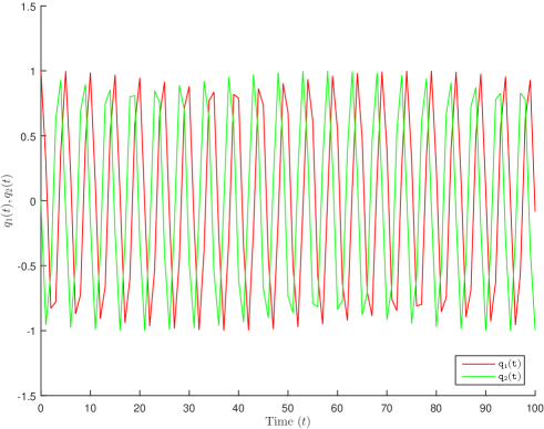
Example 1 (perturbed Kepler’s problem). Consider the Hamiltonian system studied in [24]

$$H(p,q)=\dfrac{1}{2}(p_{1}^{2}+p_{2}^{2})+\dfrac{\omega^{2}}{2}(q_{1}^{2}+q_{2}^{2})+\dfrac{\alpha}{6}(q_{1}^{2}+q_{2}^{2})^{3},$$ (7.2)

with the initial data

$$q_{1}(0)=1,\quad q_{2}(0)=0,\quad p_{1}(0)=0,\quad p_{2}(0)=\omega+\epsilon,$$

where $\alpha=\epsilon(2\omega+\epsilon)$. The analytic solution is given by

$$\begin{array}[]{l}q_{1}(t)=\cos((\omega+\epsilon)t),\quad p_{1}(t)=-(\omega+\epsilon)\sin((\omega+\epsilon)t),\\ q_{2}(t)=\sin((\omega+\epsilon)t),\quad\ p_{2}(t)=(\omega+\epsilon)\cos((\omega+\epsilon)t),\end{array}$$

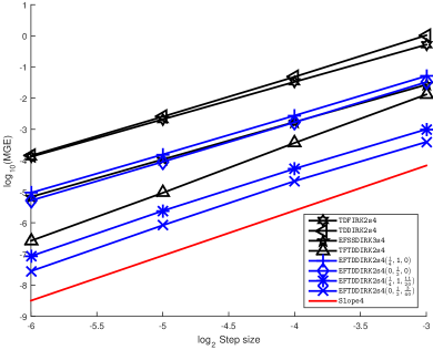
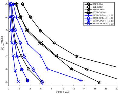
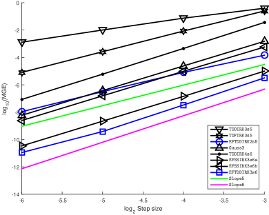
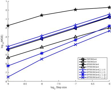
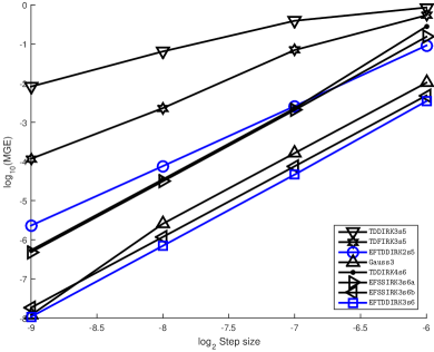
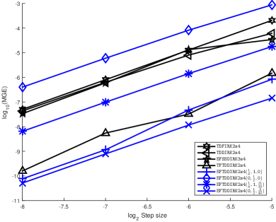
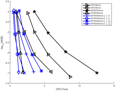
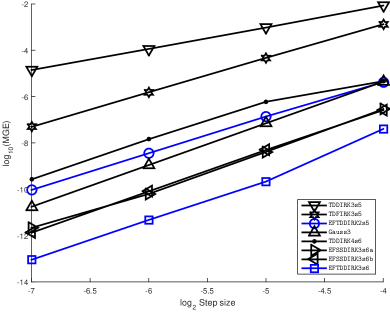
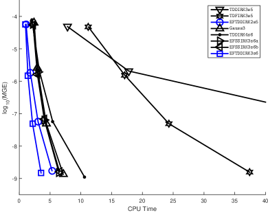
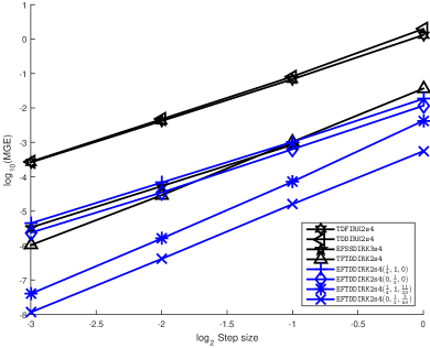
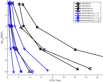
which presents oscillations (see Figure 2). In this experiment, we have chosen the parameter values $\epsilon=10^{-2}$, $\omega=5$, and the integration is carried out on the interval $[0,100]$. For accuracy comparisons, the same set of stepsizes $\{h=\frac{1}{2^{i}}$, $j=3,4,5,6\}$ is used for all the considered integrators. The numerical results are presented in Figures 3 and 4, which also show the efficiency plots (the step sizes are chosen in such a way that the same error thresholds are achieved). As seen from the left diagrams of these figures, all the new methods fully achieve their orders of convergence (4, 5, and 6).

Refer to caption
Figure 2: Solution components $q_{1}(t)$ and $q_{2}(t)$ of Example 1 showing oscillatory behavior.
Refer to caption    Refer to caption
Figure 3: Accuracy (left) and efficiency (right) plots of 4th-order methods for Example 1. For comparison, a straight line with slope 4 is added.
Refer to caption    Refer to caption
Figure 4: Accuracy (left) and efficiency (right) plots of 5th and 6th-order methods for Example 1. For comparison, straight lines with slopes 5 and 6 are added.

It can be seen from Figure 3 that the methods whose dispersion were optimized (𝙴𝙵𝚃𝙳𝙳𝙸𝚁𝙺𝟸𝚜𝟺(𝟷𝟺,𝟷,𝟷𝟷𝟸𝟶)𝙴𝙵𝚃𝙳𝙳𝙸𝚁𝙺𝟸𝚜𝟺1411120\mathtt{EFTDDIRK2s4(\tfrac{1}{4},1,\tfrac{11}{20})} and 𝙴𝙵𝚃𝙳𝙳𝙸𝚁𝙺𝟸𝚜𝟺(𝟶,𝟷𝟸,𝟹𝟺𝟶)𝙴𝙵𝚃𝙳𝙳𝙸𝚁𝙺𝟸𝚜𝟺012340\mathtt{EFTDDIRK2s4(0,\tfrac{1}{2},\tfrac{3}{40})}) clearly outperform the other methods of order 4. 
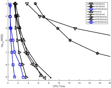
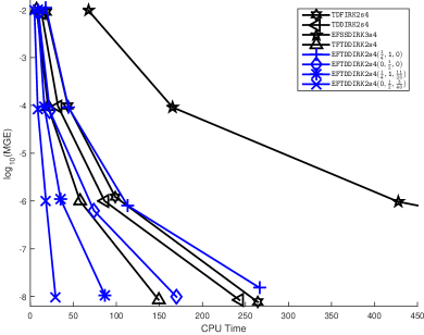
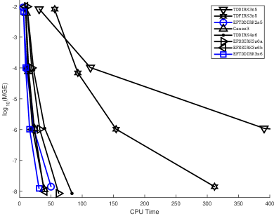
Figure 4 shows (right) that the newly derived methods 𝙴𝙵𝚃𝙳𝙳𝙸𝚁𝙺𝟸𝚜𝟻𝙴𝙵𝚃𝙳𝙳𝙸𝚁𝙺𝟸𝚜𝟻\mathtt{EFTDDIRK2s5} (order 5) and 𝙴𝙵𝚃𝙳𝙳𝙸𝚁𝙺𝟹𝚜𝟼𝙴𝙵𝚃𝙳𝙳𝙸𝚁𝙺𝟹𝚜𝟼\mathtt{EFTDDIRK3s6} (order 6) derived in this work are much more accurate and faster when compared to the considered existing methods of order 5 and 6.

Example 2 (Fermi-Pasta-Ulam problem). Next, we consider the highly oscillatory Fermi-Pasta-Ulam (FPU) problem (see [30]) including $m$ stiff springs, in which the motion is described by a second-order system of differential equations of the form

$$\ddot{x}(t)+\Omega^{2}x(t)=-\nabla U(x(t)),t\in[t_{0},t_{end}],$$ (7.3)

where

$$\Omega=\left[\begin{array}[]{ccc}{\bf 0}_{m\times m}&{\bf 0}_{m\times m}\\ {\bf 0}_{m\times m}&\omega{\bf I}_{m\times m}\end{array}\right]\qquad(\text{with}\ \omega\gg 1),$$

and $U(x)$ is a smooth nonlinear potential function given by

$$U(x)=\frac{1}{4}\big{[}(x_{1}-x_{m+1})^{4}+\sum_{j=1}^{m-1}(x_{j+1}-x_{m+j-1}-x_{j}-x_{m+j})^{4}+(x_{m}+x_{2m})^{4}\big{]}$$

with $x_{j}=x_{j}(t)$ represents for positions of the $j$th stiff spring. As in [30], we consider the case for $m=3$, and choose

$$x_{1}(0)=1,\quad\dot{x}_{1}(0)=1,\quad x_{4}(0)=\omega^{-1},\quad\dot{x}_{4}(0)=1,$$

and zero for the remaining initial values. The system is integrated on $[0,100]$ with $\omega=50$.

Note that the FPU problem (7.3) can be also described by the Hamiltonian system with total energy

$$H(x,\dot{x})=\dfrac{1}{2}\|\dot{x}\|^{2}+\dfrac{1}{2}\|\Omega x\|^{2}+U(x),$$ (7.4)

where $x$ and $\dot{x}$ expresses the scaled displacements and velocities (or momenta), respectively. Therefore, the exact value of the total energy is $H(x_{0},\dot{x}_{0})$
$=\tfrac{1}{2}(\sqrt{2})^{2}+\tfrac{1}{2}(1^{2})+(0.501200080)=2.001200080$.

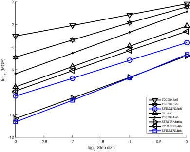
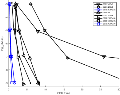
While the left diagrams of Figures 5 and 6 show the accuracy comparisons (using the same set of step sizes $\{h=1/2^{j}$, $j=6,7,8,9\}$ for each method), the right diagrams display the efficiency evaluations, in which the step sizes are chosen in such a way that the same error thresholds are achieved.

Refer to caption    Refer to caption
Figure 5: Accuracy (left) and efficiency (right) plots of 4th-order methods for Example 2.
Refer to caption    Refer to caption
Figure 6: Accuracy (left) and efficiency (right) plots of 5th and 6th-order methods for Example 2.

Among methods of order 4, one can see again that the new method $\mathtt{EFTDDIRK2s4(0,\tfrac{1}{2},\tfrac{3}{40})}$ is the most accurate and efficient. Also, the newly derived fifth- and sixth- order methods $\mathtt{EFTDDIRK2s5}$ and $\mathtt{EFTDDIRK3s6}$ are more accurate and efficient compared to some existing methods of the same order, respectively.

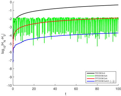
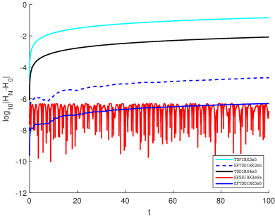
Next, we investigate the preservation of the Hamiltonian for the FPU system by some selected methods of orders 4, 5, and 6. Figure 7 presents the absolute error of the Hamiltonian ($|H_{N}-H_{0}|$) versus time using stepsize $h=\tfrac{1}{200}$, where $H_{N}$ is the computed Hamiltonian after $N$ steps.

Refer to caption    Refer to caption
Figure 7: Hamiltonian errors of 4th-order (left), 5th- and 6th-order (right) methods for Example 2.

It is observed that the most accurate methods of the new derived fourth-order methods $\mathtt{EFTDDIRK2s4(0,\tfrac{1}{2},\tfrac{3}{40}})$ preserves the Hamiltonian best. However, the newly derived fifth- and sixth-order methods $\mathtt{EFTDDIRK2s5}$ and $\mathtt{EFTDDIRK3s6}$ preserve the total energy much better than the existing methods of the same order, respectively.

Example 3 (Sine-Gordon equation). We consider the sine-Gordon nonlinear equation with periodic boundary condition (see [59])

$$\left\{\begin{array}[]{l}\dfrac{\partial^{2}u}{\partial t^{2}}=\dfrac{\partial^{2}u}{\partial x^{2}}-\sin u,\qquad-1<x<1,\quad t>0\\[8.61108pt] u(-1,t)=u(1,t).\\ \end{array}\right.$$ (7.5)

A semi-discretization in the spatial variable by the second-order centered finite difference method leads to the following system of ODEs

$$\dfrac{d^{2}U}{dt^{2}}+MU=F(U),\qquad 0<t\leq t_{end},$$ (7.6)

where $U(t)=(u_{1}(t),\ldots u_{N}(t))^{T}$ with $u_{i}(t)=u(x_{i},t)$, $i=1,\ldots,N$. Equation (7.6) can be further transformed to a system of first order DEs given by

$$\dfrac{d}{dt}\left[\begin{array}[]{c}U\\ V\\ \end{array}\right]=\left[\begin{array}[]{cc}{\bf 0}&I\\ -M&{\bf 0}\\ \end{array}\right]\left(\begin{array}[]{c}U\\ V\\ \end{array}\right)+\left[\begin{array}[]{c}\bar{0}\\ F(U)\\ \end{array}\right],\qquad 0<t\leq t_{end}.$$ (7.7)

Here, $V=U^{\prime}$, $I$ is the $N\times N$ identity matrix, 0 is the $N\times N$ zero matrix, $\bar{0}$ is a zero column vector of size $N\times 1$,

$$M=\dfrac{1}{\Delta x^{2}}\left(\begin{array}[]{ccccc}2&-1&&&-1\\ -1&2&-1&&\\ &\ddots&\ddots&\ddots&\\ &&-1&2&-1\\ -1&&&-1&2\\ \end{array}\right)$$

(with $\Delta x=2/N$, $x_{i}=-1+i\Delta x$, $i=1,2,\ldots,N$), and $F(U)=-\sin(U)=-(\sin u_{1},\ldots,\sin u_{N})T$. As in [23], we use the initial conditions

$$U(0)=(\pi)_{i=1}^{N},\qquad V(0)=\sqrt{N}\left(0.01+\sin\left(\dfrac{2\pi i}{N}\right)\right)_{i=1}^{N},$$

($N=64$) and integrate the problem on the interval $[0,10]$.

Refer to caption    Refer to caption
Figure 8: Accuracy (left) and efficiency (right) plots of 4th-order methods for Example 3.
Refer to caption    Refer to caption
Figure 9: Accuracy (left) and efficiency (right) plots of 5th and 6th-order methods for Example 3.

Again, on the left side of Figure 8 we display accuracy plots using the same set of stepsizes $h=1/2^{i}$, $i=6,7,8,9$, and the efficiency plots are shown on the right side (different time step sizes were chosen so that all the compared methods attain about the same level of accuracy).

The numerical results show that $\mathtt{EFTDDIRK2s4(0,\tfrac{1}{2},0)}$ is the least accurate but the most efficient among the tested methods. This can be explained by the fact that its first stage is computed explicitly (since $c_{1}=0$). One can also see that the optimized fourth-order method $\mathtt{EFTDDIRK2s4(0,\tfrac{1}{2},\tfrac{3}{40})}$ performs the best overall compared to other fourth-order methods.

Next, we also investigate the spatial grid effect on this problem. For this, we compare the maximum global error obtained by all the methods for different values of $N$ (25, 50, and 100) with stepsize $h=\tfrac{1}{16}$ at time $t=10$. We present the obtained results in Tables 3 and 4. From these results, we observe that the accuracy decreases when increasing $N$. This is due to the stiffness of the problem which is increasing for larger spatial grid sizes $N$, which consequently affects to the global error.

Method $N=25$ $N=50$ $N=100$
$\mathtt{TDDIRK2s4}$ $1.05\cdot 10^{-4}$ $1.00\cdot 10^{-3}$ $2.76\cdot 10^{-2}$
$\mathtt{TDFIRK2s4}$ $1.45\cdot 10^{-4}$ $1.60\cdot 10^{-3}$ $1.04\cdot 10^{-2}$
$\mathtt{EFSSDIRK3s4}$ $6.15\cdot 10^{-5}$ $9.18\cdot 10^{-4}$ $3.20\cdot 10^{-3}$
$\mathtt{TFTDDIRK2s4}$ $4.07\cdot 10^{-7}$ $1.34\cdot 10^{-5}$ $1.27\cdot 10^{-5}$
$\mathtt{EFTDDIRK2s4(\tfrac{1}{4},1,0)}$ $7.35\cdot 10^{-7}$ $4.29\cdot 10^{-5}$ $1.71\cdot 10^{-4}$
$\mathtt{EFTDDIRK2s4(0,\tfrac{1}{2},0)}$ $1.00\cdot 10^{-3}$ $7.69\cdot 10^{-4}$ $3.00\cdot 10^{-3}$
$\mathtt{EFTDDIRK2s4(\tfrac{1}{4},1,\tfrac{11}{20})}$ $1.64\cdot 10^{-5}$ $1.78\cdot 10^{-4}$ $5.58\cdot 10^{-4}$
$\mathtt{EFTDDIRK2s4(0,\tfrac{1}{2},\tfrac{3}{40})}$ $2.47\cdot 10^{-7}$ $3.09\cdot 10^{-6}$ $2.34\cdot 10^{-5}$
Table 3: Errors for 4th-order methods for different values of $N$ using $h=\tfrac{1}{16}$.
Method $N=25$ $N=50$ $N=100$
$\mathtt{TDDIRK3s5}$ $1.80\cdot 10^{-4}$ $1.40\cdot 10^{-3}$ $4.62\cdot 10^{-2}$
$\mathtt{TDFIRK3s5}$ $8.59\cdot 10^{-6}$ $8.29\cdot 10^{-5}$ $1.06\cdot 10^{-2}$
$\mathtt{EFTDDIRK2s5}$ $6.46\cdot 10^{-8}$ $5.83\cdot 10^{-7}$ $4.64\cdot 10^{-5}$
$\mathtt{Gauss3}$ $9.76\cdot 10^{-8}$ $1.92\cdot 10^{-6}$ $1.16\cdot 10^{-5}$
$\mathtt{TDDIRK4s6}$ $1.07\cdot 10^{-6}$ $2.21\cdot 10^{-5}$ $6.63\cdot 10^{-4}$
$\mathtt{EFSSIRK3s6a}$ $6.79\cdot 10^{-9}$ $4.48\cdot 10^{-8}$ $7.56\cdot 10^{-7}$
$\mathtt{EFSSIRK3s6b}$ $3.38\cdot 10^{-9}$ $1.07\cdot 10^{-7}$ $2.01\cdot 10^{-6}$
$\mathtt{EFTDDIRK3s6}$ $1.28\cdot 10^{-9}$ $6.79\cdot 10^{-9}$ $1.64\cdot 10^{-7}$
Table 4: Errors for 5th- and 6th-order methods for different values of $N$ using $h=\tfrac{1}{16}$.

Example 4 (An “almost” periodic orbit problem). Lastly, we consider the almost periodic orbit problem studied in [52] given by

$$y^{\prime\prime}+y=0.001{\rm e}^{{\rm i}x},\quad y(0)=1,\quad y^{\prime}(0)=0.9995i,$$

whose analytical solution is given by

$$y(x)=(\cos x+0.0005x\sin x)+{\rm i}(\sin x-0.0005x\cos x),$$

which represent a motion on a perturbation of a circular orbit in the complex plane. Clearly, for this problem $\omega=1$.

We integrate the problem on $[0,1000]$ using all the methods listed above. Numerical results were obtained for all the methods using stepsizes $h=1/2^{n}$, $n=0,1,2,3$ and are illustrated in Figures 10 and 11.

Refer to caption    Refer to caption
Figure 10: Accuracy (left) and efficiency (right) plots of 4th-order methods for Example 4.
Refer to caption    Refer to caption
Figure 11: Accuracy (left) and efficiency (right) plots of 5th and 6th-order methods for Example 4.

In view of Figures 10 and 11, the methods whose dispersion were optimized ($\mathtt{EFTDDIRK2s4(\tfrac{1}{4},1,\tfrac{11}{20})}$ and $\mathtt{EFTDDIRK2s4(0,\tfrac{1}{2},\tfrac{3}{40})}$) clearly outperform the other methods of order 4. Besides, we observe clearly from efficiency curves of Figures 10 and 11 that the newly derived methods $\mathtt{EFTDDIRK2s5}$ (order 5) and $\mathtt{EFTDDIRK3s6}$ (order 6) derived in this work are much more accurate and faster when compared to the considered existing methods.

8 Conclusion

We have derived a class of exponentially fitted two-derivative diagonally implicit Runge–Kutta (EFTDDIRK) methods for solving oscillatory differential equations. New order and exponential fitting conditions are obtained, leading to the derivation of new methods of orders 4, 5, and 6. Stability and phase-lag analysis of these methods were investigated which resulted in optimized fourth-order schemes that are much more accurate and efficient. Our numerical experiments have confirmed the efficiency and accuracy of these new EFTDDIRK methods when compared to standard implicit (two-derivative) Runge–Kutta methods of the same orders.

Future works will be focusing on the existence of symmetric EFTDDIRK methods for symplectic, Hamiltonian or reversible systems. Also, we will consider the two-derivative singly diagonally implicit methods with a view to practical applications because of the easy implementation structure as discussed in [10] and [37].

Acknowledgements

J.O. Ehigie is grateful for the financial support of EMS-Simons for Africa program, which enabled him undertake some aspect of this research at Southern Methodist University, TX, USA. V.T. Luan gratefully acknowledges the support of the National Science Foundation under grant NSF DMS–2012022. X. You would like to acknowledge the support of the National Natural Science Foundation of China (No. 11171155, No. 11871268) and Natural Science Foundation of Jiangsu Province, China (No. BK20171370).

References

  • [1] A. Abdi, M. Bras, G. Hojjati, On the construction of second derivative diagonally implicit multistage integration methods, Appl. Numer. Math. 76 (2014) 1–18.
  • [2] A. Abdi, G. Hojjati, Maximal order of second derivative general linear methods with Runge–Kutta stability, Appl. Numer. Math. 61 (2011) 1046–1058.
  • [3] A. Abdi, G. Hojjati, Implementation of Nordsieck second derivative methods for stiff ODEs, Appl. Numer. Math. 94 (2015) 241–253.
  • [4] N.A. Ahmad, N. Senu, Z.B. Ibrahim, M. Othman, Diagonally implicit two derivative Runge Kutta methods for solving first order initial value problems, JACM 4(1) (2019) 18–36.
  • [5] N.A. Ahmed, N. Senu, Z.B. Ibrahim, M. Othman, Trigonometrically-fitted diagonally implcit two-derivative Runge-Kutta method for numerical solution of periodic ivps. ASM Sc. J. Special Issue I, IQRAC2018, (2019) 50–59.
  • [6] M.A. Akanbi, S.A. Okunuga, A.B. Sofoluwe, Step size bounds for a class of multiderivative explicit Runge–Kutta methods, Modeling and Simulation in Engineering, Economics and Management, Springer Berlin Heidelberg (2012), 188–197.
  • [7] R. Alexander, Diagonally implicit Runge–Kutta methods for Stiff ODEs, SIAM J. Numer. Anal., 14(6) (1973) 1006–1021.
  • [8] V.I. Arnold, Mathematical methods of classical mechanics, Springer-Verlag, New York, 1989.
  • [9] D.G. Bettis. Runge–Kutta algorithms for oscillatory problems. J. Appl. Math. Phys. (ZAMP) 30 (1979) 699–704.
  • [10] J.C. Butcher, Numerical methods for ordinary differential equations, Third Edition, John Wiley & Sons Ltd, 2016.
  • [11] J.C. Butcher, G. Hojjati, Second derivative methods with RK stability, Numer. Algor. 40 (2005) 415–429.
  • [12] M. Calvo, J.M. Franco, J.I. Montijano, L. Randez, Sixth-order symmetric and symplectic exponentially fitted modified Runge-Kutta of Gauss type, Comput. Phys. Commun. 178 (2008) 732–744.
  • [13] M. Calvo, J.M. Franco, J.I. Montijano, L. Randez, Sixth-order symmetric and symplectic exponentially fitted Runge-Kutta methods of the Gauss type, J. Comput. Appl. Math. 233 (2009) 387–398.
  • [14] R.P.K. Chan, A.Y. Tsai, On explicit two-derivative Runge- Kutta methods, Numer. Algor. 53 (2010) 171–194.
  • [15] R.P.K. Chan, S. Wang, A.Y.J. Tsai, Two-derivative Runge–Kutta methods for differential equations, AIP Conference Proceedings 1479, 262, (2012).
  • [16] Z. Chen, J. Li, R. Zhang, X. You, Exponentially fitted two-derivative Runge–Kutta methods for simulation of oscillatory genetic regulatory systems, Comput. Math. Methods Med. 2015 Article ID 689137, (2015).
  • [17] J.P. Coleman, Numerical methods for $y^{\prime\prime}=f(x,y)$ via rational approximations for the cosine, IMA J. Numer. Anal. 9 (1989) 145–165.
  • [18] J.O. Ehigie, D. Diao, R. Zhang, Y. Fang, X. Hou, X. You, Exponentially fitted symmetric and symplectic DIRK methods for oscillatory Hamiltonian systems, J. Math. Chem. 56 (2018) 1130–1152.
  • [19] M.B. Elowitz MB, S. A. Leibler. A synthetic oscillatory network of transcriptional regulators, Nature, 403, (2000), 335–338.
  • [20] Y. Fang Y, X. You, New optimized two-derivative Runge–Kutta type methods for solving the radial Schrödinger equation, J. Math. Chem. 52 (2014) 240–254.
  • [21] Y. Fang Y, X. You, Q. Ming, Trigonometrically fitted two-derivative Runge–Kutta methods for solving oscillatory differential equations, Numer. Algor. 65 (2014) 651–667.
  • [22] J.M. Franco, I. Gómez, Fourth-order symmetric DIRK methods for periodic stiff problems, Numer. Algor. 32 (2003) 317–336.
  • [23] J.M. Franco, New methods for oscillatory systems based on ARKN methods, Appl. Numer. Math. 56, (2006), 1040-1053.
  • [24] J.M. Franco, I. Gómez. Symplectic explicit methods of Runge–Kutta-Nyström type for solving perturbed oscillators, J. Comput. Applied Math. 260 (2014) 482–493.
  • [25] W. Gautschi, Numerical integration of ordinary differential equations based on trigonometric polynomials, Numer. Math. 3 (1961), 381–397.
  • [26] D. Goeken. O. Johnson, Runge–Kutta with higher order derivative approximations, Appl. Numer. Math. 34 (2000), 207–218.
  • [27] M. Griebel, S. Knapek, G. Zumbusch, Numerical simulation in molecular dynamics: numerics, algorithms, parallelizations, applications, Springer (2007).
  • [28] E. Hairer, S.P. Nørsett, G. Wanner, Solving ordinary differential equations I: Non stiff problems, Springer-Verlag, 1993.
  • [29] E.  Hairer and G.  Wanner, Solving Ordinary Differential Equations II, Stiff and Differential-Algebraic Problems, 2nd rev. ed., Springer, New York, 1996.
  • [30] E. Hairer, Ch. Lubich, G. Wanner, Geometric mumerical integration–Structure preserving algorithms for ordinary differential equations, 2nd edition, Springer, Berlin, 2006.
  • [31] M.  Hochbruck, A. Ostermann, Exponential Integerators, Acta Numerica, 19 (2010), 209–286.
  • [32] L. Ixaru, Numerical methods for differential equations and applications, Reidel, Dordrecht, Boston, Lancaster, 1984.
  • [33] L. Ixaru, G. Vanden Berghe, Exponential Fitting, Kluwer Academic Publishers, 2004.
  • [34] L. Ixaru, G. Vanden Berghe, H. De Meyer, Frequency evaluation in exponential fitting multistep algorithms for ODEs, J. Comput. Appl. Math. 140 (2002) 423–434
  • [35] Z. Kalogiratou, T. Monovasilis, T.E. Simos, Two-derivative Runge–Kutta methods with optimal phase properties, Math. Meth. Appl. (2019) 1–11.
  • [36] K. Kastlunger, G. Wanner, On Turan type implicit Runge–Kutta methods, Computing 9 (1972) 317–325.
  • [37] C.A. Kennedy, M.H. Carpenter. Diagonal implicit Runge–Kutta methods for ordinary differential equations. A Review, NASA Research report, NASA-TM-2016-219173, 2016. http://www.sti.nasa.gov.
  • [38] G.V. Krivovichev, Optimized low-dispersion and low dissipation two-derivative Runge-Kutta method for wave equations. J. Appl. Math. Comput. 63 (2020) 787–811.
  • [39] V.T. Luan, D.L. Michels, Efficient exponential time integration for simulating nonlinear coupled oscillators, J. Comput. Appl. Math. 391 (2021) 113429.
  • [40] V.T. Luan, Efficient exponential Runge–Kutta methods of high order: construction and implementation, BIT (2021), 1–26.
  • [41] V.T. Luan, Fourth-order two-stage explicit exponential integrators for time-dependent PDEs, Appl. Numer. Math., 112 (2017), 91–103.
  • [42] V.T. Luan, A. Ostermann, Exponential Runge–Kutta methods of high-order for parabolic problems, J. Comput. Appl. Math, 256 (2014), 168–179.
  • [43] V.T. Luan, A. Ostermann, Exponential B-series: The stiff case, SIAM J. Numer. Anal., 51(6) (2013), 3431–3445.
  • [44] V.T. Luan, A. Ostermann, Parallel exponential Rosenbrock methods, Computers & Mathematics with Applications, 71(5) (2016), 1137–1150.
  • [45] T. Lyche. Chebyshevian multistep methods for ordinary differential equations. Numer. Math. 19 (1972) 65–75.
  • [46] B. Paternoster, Present state-of-the-art in exponential fitting. A contribution dedicated to Liviu Ixaru on his 70th birthday, Comput. Phys. Commun. 183 (2012) 2499–2512.
  • [47] W.H. Press, S.A. Teukolsky, W.T. Vetterling, B.P. Flannery. Numerical recipes: the art of scientific computing, Cambridge University Press, England, 2007.
  • [48] H. Ramos and J. Vigo-Aguiar, On the frequency choice in trigonometrically fitted methods, Appl. Math. Lett. 23(11) (2010) 1378–1381.
  • [49] F. Rossi, M. A. Budroni, N. Marchettini, L. Cutietta, M. Rustici, M. L. T. Liveri. Chaotic dynamics in an unstirred ferroin catalyzed Belousov-Zhabotinsky reaction, Chem. Phys. Lett. 480(4), (2009) 322–326.
  • [50] D.C. Seal, Y. Guclu. A.J. Christlieb, High-order multiderivative time integrators for hyperbolic conservation laws, J. Sci. Comput. 60 (2014) 101–140.
  • [51] T.E. Simos, An exponentially-fitted Runge–Kutta method for the numerical integration of initial-value problems with periodic or oscillating solutions, Comput. Phys. Commun. 115 (1998) 1–8.
  • [52] E. Steifel, D.G. Bettis. Stabilization of Cowell’s method, Numer. Math. 13 (1969) 154–175.
  • [53] A.Y.J. Tsai, R.P.K. Chan, S. Wang. Two derivative Runge-Kutta methods for PDEs using a novel discretization approach, Numer. Algor. 65(3) (2014) 697–703.
  • [54] M.O. Turaci, T. Ozis. Derivation of three-derivative Runge-Kutta methods, Numer. Algor. 74(1) (2017) 247–265.
  • [55] G. Vanden Berghe, H. De Meyer, M. Van Daele, T. Van Hecke. Exponentially-fitted explicit Runge–Kutta methods, Comp. Phys. Commun. 123 (1999) 7–15.
  • [56] G. Vanden Berghe, H. De Meyer, M. Van Daele, T. Van Hecke. Exponentially-fitted Runge–Kutta methods, J. Comput. Appl. Math. 125 (2000) 107–115.
  • [57] J. Vigo-Aguiar, H. Ramos. On the choice of the frequency in trigonometrically-fitted methods for periodic problems, J. Comput. Appl. Math. 277 (2015) 94–105.
  • [58] H. Van de Vyver, Stability and phase-lag analysis of explicit Runge–Kutta methods with variable coefficients for oscillatory problems, Comput. Phys. Commun. 173 (2005) 115–130.
  • [59] H.F. Weinberger, A first course in partial differential equations with complex variables and transform methods, Dover Publications, New York, 1965.
  • [60] A.S. Wusu, M.A. Akanbi, S.A. Okunuga, A three-stage multiderivative explicit Runge–Kutta method, American Journal of Computational Mathematics. 3 (2013) 121–126.
  • [61] X. Wu, J. Xia, Extended Runge–Kutta-like formulae, Applied Numerical Mathematics. 56 (2006) 1584–1605.
  • [62] X. Wu, X. You, B. Wang, Structure preserving algorithms for oscillatory differential equations, Science Press, Beijing and Springer, Berlin, 2013.