ACFI-T20-18 CP-violating Higgs Di-tau Decays: Baryogenesis and Higgs Factories

Abstract

We demonstrate how probes of CP-violating observables in Higgs di-tau decays at prospective future lepton colliders could provide a test of weak scale baryogenesis with significant discovery potential. Measurements at the Circular Electron Positron Collider, for example, could exclude a CP phase larger than $2.9^{\circ}$ ($5.6^{\circ}$) at 68% (95%) C.L. assuming the Standard Model value for magnitude of the tau lepton Yukawa coupling. Conversely, this sensitivity would allow for a $5\,\sigma$ discovery for 82% of the CP phase range $[0,2\pi)$. The reaches of the Future Circular Collider - ee and International Linear Collider are comparable. As a consequence, future lepton colliders could establish the presence of CP violation required by lepton flavored electroweak baryogenesis with at least $3\,\sigma$ sensitivity. Our results illustrate that Higgs factories are not just precision machines but can also make $\mathcal{O}(1)$ measurement of the new physics beyond the Standard Model.

1 Introduction

The discovery of the Higgs boson at the Large Hadron Collider (LHC) [1, 2] and subsequent measurements of its properties strongly favor the mechanism of electroweak symmetry-breaking (EWSB) given by the Standard Model (SM) of particle physics. In particular, the SM predicts each Higgs boson-fermion Yukawa coupling to be purely real, with magnitude proportional to the fermon mass. However, LHC measurements have confirmed this prediction up to only $\mathcal{O}(10)\%$ precision [3, 4, 5, 6] , leaving considerable room for physics beyond the Standard Model (BSM) in Higgs boson-fermion interactions. Precision Higgs boson studies aim to explore these BSM possibilities. Proposed future lepton colliders, including the Circular Electron-Positron Collider (CEPC) [7], Future Circular Collider (FCC)-ee [8], and International Linear Collider (ILC) [9], are designed for this purpose.

The motivations for BSM Higgs interactions are well known, including solutions to the hierarchy problem, generation of neutrino mass, dark matter, and the cosmic baryon asymmetry (BAU). In what follows, we focus on the possibility that the observation of CP-violating effects in Higgs-tau lepton interactions at a future lepton collider could provide new insight into the BAU problem. As pointed out by Sakharov[10], a dynamical generation of the BAU requires three ingredients in the particle physics of the early universe: : (1) non-conserving baryon number (2) out-of-equilibrium dynamics (assuming CPT conservation) and (3) C and CP violation. While the SM contains the first ingredient in the form of electroweak sphalerons, it fails to provide the needed out-of-equilibrium conditions and requisite CP-violation. The presence of BSM physics in the dynamics of EWSB could remedy this situation – the electroweak baryogenesis (EWBG) scenario (for a recent review, see, Ref. [11]). While flavor-diagonal CP-violating (CPV) interactions relevant to EWBG are strongly constrained by limits on permanent electric dipole moments (EDMs) of the electron, neutron, and neutral atoms [12, 13] , the landscape for flavor non-diagonal CPV is less restricted. Here, we show that searches for CPV effects in the Higgs di-tau decays at future lepton colliders could provide an interesting probe of “flavored EWBG” [14, 15, 16, 17, 18] in the lepton sector.

In addition to being theoretically well-motivated in its own right, EWBG has the additional attraction of experimental testability. Modifications of the SM scalar sector necessary for the EWBG out-of-equilibrium conditions provide a rich array of signatures accessible at the LHC and prospective future colliders [19]. The signatures of CP violation could appear in either low- or high-energy experiments. Our present focus is on the possible modification of the the $\tau$ Yukawa coupling by a nonzero CP phase $\Delta$ as defined in Eq. (2.1) below and the resulting impact on Higgs decay into a pair of $\tau$ leptons. In this context, it has been known for some time that the $\Delta$ phase can be measured at colliders [20, 21, 32, 22, 23, 24, 25, 26, 27, 28, 29, 30, 31]. An $\mathcal{O}(1)$ modulation in the relevant differential distribution allows very accurate determination of $\Delta$. The measurements at LHC can achieve a precision around 10^∘[33, 34, 35, 36, 37, 38] at 95% confidence level (C.L.) by using the full data with 3 ab^-1 of integrated luminosity. Future lepton colliders [39] can further improve the measurements with higher integrated luminosity, optimized energy for Higgs production, and cleaner environment. Indeed, it was shown that the projected sensitivity for the ILC can reach $4.3^{\circ}$ [40] and $2.9^{\circ}$ for the CEPC [41] at $1\,\sigma$ level. To our knowledge, a detailed study connecting this sensitivity to the BAU has yet to appear in the literature.

In this work we thus study the capability of the CEPC, FCC-ee and ILC in probing $\Delta$ and the resulting prospects of testing lepton flavored EWBG scenario. The projected sensitivities at future lepton colliders are much better than the current LHC results [42]. In Sec. 2, we first make detailed comparison of several observables (the neutrino azimuthal angle difference $\delta\phi_{\nu}$, the polarimeter $\delta\phi_{r}$, the acoplanarity $\phi^{*}$, and the $\Theta$ variable) to show that the polarimeter [32, 43] is not just the optimal choice for probing $\Delta$ but can also apply universally to both the $\tau\rightarrow\pi\nu$ and $\tau\rightarrow\rho\nu$ decay channels. Then we use a simplified smearing scheme to simulate the detector responses and use $\chi^{2}$ minimization to find the physical solution of neutrino/tau momentum in Sec. 3. Based on these, we find that the future lepton colliders can make $5\,\sigma$ discovery of a nonzero CP phase for 82% of the allowed range. With a combination of these channels, the $1\,\sigma$ sensitivities can reach $2.9^{\circ},3.2^{\circ}$, and $3.8^{\circ}$ at the CEPC, FCC-ee, and ILC, respectively. Our result is better than the previous study for the ILC [40] and the same as Ref. [41] for the CEPC. Notice that although the leptonic decay mode of $\tau$ is also considered in addition to the two meson decay modes with more usable events, a matrix element based observable is adopted [41] instead of the polarimeter $\delta\phi_{r}$ as we do here, leading to accidentally the same result as ours. Finally, in Sec. 4, we follow Ref. [14] in analyzing the implications for lepton flavored EWBG scenario with $3\,\sigma$ sensitivity for the presence of CP violation at the CEPC, FCC-ee and ILC. We summarize our findings in Sec. 5.

2 CP Phase and Azimuthal Angle Distributions

The SM predicts the Higgs couplings with other SM particles to be proportional to their masses, including the $\tau$ lepton, $-y_{\tau}/\sqrt{2}\bar{\tau}_{L}\tau_{R}h+\mathrm{h.c.}=-m_{\tau}/v\bar{\tau}\tau h$ , where $h$ denotes the SM-like Higgs boson, $v=246$ GeV is the vacuum expectation value (VEV) and $m_{\tau}$ is the tau lepton mass. Although $y_{\tau}$ is in general complex, its CP phase can be rotated away without leaving any physical consequences. However, this is not always true when going beyond the SM. Any deviation from the SM prediction, for either the $\tau$ Yukawa coupling magnitude or the CP phase, indicates new physics. We first study the CP phase measurement by explicitly comparing various definitions of differential distributions in this section and then the detector response behaviors in Sec. 3. The influence of the Yukawa coupling magnitude deviation from the SM prediction will be discussed in later parts of this paper.

The $\tau$ Yukawa coupling can be generally parametrized as

$$\mathcal{L}_{h\tau\tau}=-\kappa_{\tau}\dfrac{m_{\tau}}{v}\bar{\tau}(\cos\Delta+i\gamma_{5}\sin\Delta)\tau h$$ (2.1)

with $\kappa_{\tau}$ being real and positive by definition, and $\Delta\in[0,2\pi)$ in general. We will consider $\Delta\in[0,\pi]$ since the CP measurement is insensitive to the multiplication of $\kappa_{\tau}$ by $-1$ [33]. The SM prediction for $\tau$ Yukawa coupling can be recovered with $\kappa_{\tau}\rightarrow 1$ and $\Delta\rightarrow 0$. A non-zero value of the CP phase $\Delta$ indicates CP violation in the $\tau$ Yukawa coupling and can be connected to baryogenesis in the early Universe [14].

Because of the P- and T- violating nature of the second term in Eq. (2.1), the spin correlation among the two $\tau$ leptons from a Higgs decay is an especially interesting probe for constraining its value [23]. In practice, one cannot measure the $\tau$ lepton directly but must rely on its decay products. The two most promising channels are the $\tau$ decay into $\pi^{\pm}$ ($\tau^{\pm}\rightarrow\pi^{\pm}\nu_{\tau^{\pm}}$) and into $\rho^{\pm}$ ($\tau^{\pm}\rightarrow\rho^{\pm}\nu_{\tau^{\pm}}\rightarrow\pi^{\pm}\pi^{0}\nu_{\tau^{\pm}}$ ) with $\nu_{\tau^{-}}(\nu_{\tau^{+}})$ being the neutrino (anti-neutrino) from the decay of $\tau^{-}(\tau^{+})$. These two channels contribute 10.82% and 25.49% of a single $\tau$ decay branching fractions [44], respectively.

2.1 Observables

For each $\tau$ decay, one decay plane can be formed by its decay products. The generic azimuthal angle $\phi$ difference between the two decay planes is then a good observable for probing $\Delta$, which can be expressed as

$$\frac{1}{\Gamma}\frac{d\Gamma}{d\delta\phi}=\frac{1}{2\pi}\left[1+A\cos(2\Delta-\delta\phi)\right]\;,$$ (2.2)

where the coefficient $A$ depends on the choice of observable. Note that only for $\Delta$ differing from integer multiples of $\pi/2$, this distribution will contain a term odd in $\delta\phi$. There exist a variety of observables that afford access to $\Delta$, which appears as the azimuthal angle difference in two decay planes. Here we review several possibilities and discuss the rationale for our choice of one of them.

Neutrino azimuthal angle difference. For both $\tau$ leptons decaying into a single charged pion, $\tau^{\pm}\rightarrow\pi^{\pm}\nu_{\tau^{\pm}}$, the differential distribution of the neutrino momentum azimuthal angle difference [43] is

$$\frac{1}{\Gamma}\frac{d\Gamma(h\rightarrow\pi^{+}\pi^{-}\nu_{\tau}\overline{\nu}_{\tau})}{d\delta\phi_{\nu}}=\frac{1}{2\pi}\left[1-\frac{\pi^{2}}{16}\cos(2\Delta-\delta\phi_{\nu})\right]\ \ \ ,$$ (2.3)

where $\delta\phi_{\nu}\equiv\phi_{\nu}-\phi_{\overline{\nu}}$ and $\phi_{\nu}(\phi_{\overline{\nu}})$ are defined in the $\tau^{-}(\tau^{+})$ rest frame. On the other hand, if both $\tau$’s decay to rho mesons, $\tau^{\pm}\to\rho^{\pm}(\rightarrow\pi^{\pm}+\pi^{0})\nu_{\tau^{\pm}}$, the differential distribution of the neutrino azimuthal angle difference $\delta\phi_{\nu}$ becomes,

$$\frac{1}{\Gamma}\frac{d\Gamma(h\rightarrow\rho^{+}\rho^{-}\nu_{\tau}\overline{\nu}_{\tau})}{d\delta\phi_{\nu}}=\frac{1}{2\pi}\left[1-\frac{\pi^{2}}{16}\left(\frac{m_{\tau}^{2}-2m_{\rho}^{2}}{m_{\tau}^{2}+2m_{\rho}^{2}}\right)^{2}\cos(2\Delta-\delta\phi_{\nu})\right]$$ (2.4)

with a non-negligible suppression factor, $(m_{\tau}^{2}-2m_{\rho}^{2})^{2}/(m_{\tau}^{2}+2m_{\rho}^{2})^{2}\sim 0.2$. As shown in Fig. 1, this significantly reduces the sensitivity to the CP phase $\Delta$. The neutrino azimuthal angle difference $\delta\phi_{\nu}$ is a good observable for the $\tau\rightarrow\pi\nu_{\tau}$ decay, but not for the $\tau\rightarrow\rho\nu_{\tau}$ channel.

Polarimeter. Since the azimuthal angle difference is not necessarily the optimized choice and multiple definitions of azimuthal angle have been invented. In Refs. [43, 32, 40], the azimuthal angle difference between the polarimeter vectors ${\bf r}_{\pm}$ was studied. For the $\tau$ decays, the polarimeter vectors are defined as

$$\tau^{\pm}\rightarrow\pi^{\pm}\nu_{\tau^{\pm}} : {\bf r}_{\pm}\equiv-\hat{{\bf p}}_{\nu_{\tau^{\pm}}},$$ (2.5a)

$$\tau^{\pm}\rightarrow\rho^{\pm}(\to\pi^{\pm}\pi^{0})\nu_{\tau^{\pm}} : {\bf r}_{\pm}\equiv-\frac{1}{N_{\pm}}\left[\hat{{\bf p}}_{\nu_{\tau^{\pm}}}+\frac{2m_{\tau}}{m^{2}_{\rho}-4m^{2}_{\pi}}\frac{E_{\pi^{\pm}}-E_{\pi^{0}_{\pm}}}{E_{\pi^{\pm}}+E_{\pi^{0}_{\pm}}}\left({\bf p}_{\pi^{\pm}}-{\bf p}_{\pi^{0}_{\pm}}\right)\right],\qquad$$ (2.5b)

where ${\bf r}_{\pm}$ is calculated in the corresponding $\tau^{\pm}$ rest frame, $(E_{\pi^{0}_{\pm}},{\bf p}_{\pi^{0}_{\pm}})$ is the $\pi^{0}$ momentum in the $\tau^{\pm}$ decay, and $N_{\pm}$ is a normalization factor to ensure $|{\bf r}_{\pm}|=1$. Then the differential distribution in Eq. (2.2) becomes

$$\frac{1}{\Gamma}\frac{d\Gamma}{d\delta\phi_{r}}=\frac{1}{2\pi}\left[1-\frac{\pi^{2}}{16}\cos(2\Delta-\delta\phi_{r})\right],$$ (2.6)

for both decay channels including the mixed mode, $h\rightarrow\rho^{\pm}\pi^{\mp}\nu_{\tau}\overline{\nu}_{\tau}$. From the neutrino azimuthal angle difference $\delta\phi_{\nu}$ in Eq. (2.4) to the one of the polarimeter in Eq. (2.6), the amplitude gets amplified by a factor of 5 which is a significant improvement.

The azimuthal angle difference $\delta\phi_{r}\equiv\phi_{{\bf r}_{+}}-\phi_{{\bf r}_{-}}$ is defined with respect to the $z$ direction, ${\bf z}\equiv{\hat{\bf p}}_{\tau^{-}}$. In the Higgs rest frame,

$$\tan\delta\phi_{r}=\frac{{\hat{\bf p}}_{\tau^{-}}\cdot({\bf r}_{+}\times{\bf r}_{-})}{{\bf r}_{-}\cdot{\bf r}_{+}-({\bf r}_{+}\cdot{\hat{\bf p}}_{\tau^{-}})({\bf r}_{-}\cdot{\hat{\bf p}}_{\tau^{-}})}.$$ (2.7)

For the $\tau^{\pm}\rightarrow\pi^{\pm}\nu_{\tau^{\pm}}$ decay channel, the polarimeter is along the neutrino momentum direction, namely, ${\bf r}_{\pm}=-\hat{\bf p}_{\nu_{\tau^{\pm}}}$ as shown in Eq. (2.5a). When di-tau decay into pions it is the azimuthal angle difference $\phi_{\nu}$. In contrast, the polarimeter for the $\tau^{\pm}\rightarrow\rho^{\pm}\nu_{\tau^{\pm}}$ decay channel does not coincide with any momentum of the final-state particles. For illustration, the distribution of $\delta\phi_{r}$ for $h\to\tau^{+}(\rightarrow\rho^{+}\bar{\nu}_{\tau})\tau^{-}(\rightarrow\rho^{-}\nu_{\tau})$ is shown in Fig. 1.

The 4-vector $r_{\pm}=(0,{\bf r_{\pm}})$ serves as the effective spin of the corresponding $\tau^{\pm}$ leptons. This becomes evident in the total matrix element of the Higgs decay chain,

$$|\mathcal{M}^{\rm total}|^{2} \propto {\rm Tr}\left[\left(\not{p}_{\tau^{-}}+m_{\tau}\right)\left(1+\gamma_{5}\not{r}_{-}\right)\mathcal{O}\left(\not{p}_{\tau^{+}}-m_{\tau}\right)\left(1-\gamma_{5}\not{r}_{+}\right)\overline{\mathcal{O}}\right],$$ (2.8)

with $\mathcal{O}\equiv\cos\Delta+i\gamma_{5}\sin\Delta$, $\overline{\mathcal{O}}\equiv\gamma^{0}\mathcal{O}^{\dagger}\gamma^{0}$ and $p_{\tau^{\pm}}\equiv(E_{\tau^{\pm}},{\bf p}_{\tau^{\pm}})$ being the momentum of $\tau^{\pm}$. If the Higgs boson decays to polarized $\tau$ leptons, it should be the $\tau$ spin vector $s_{\pm}=(|{\bf p}_{\tau^{\pm}}|/m_{\tau},E_{\tau^{\pm}}/m_{\tau}{\hat{\bf p}_{\tau^{\pm}}})$ that appears in place of the polarimeter $r_{\pm}$. But since the Higgs decay chain also contains contribution from the $\tau$ decays, $s_{\pm}$ is replaced by $r_{\pm}$ to take the extra effects into consideration.

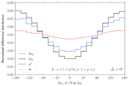
Fig. 1: The differential distributions of $h\to\tau^{+}(\rightarrow\rho^{+}\bar{\nu}_{\tau})\tau^{-}(\rightarrow\rho^{-}\nu_{\tau})$ for neutrino momentum $\delta\phi_{\nu}$ (red), polarimeter $\delta\phi_{r}$ (black), acoplanarity $\phi^{*}$ (blue), and the $\Theta$ variable (green) at the truth level for $\Delta=0^{\circ}$.

Acoplanarity. This observable was introduced in Ref. [22, 23] for the $\tau\rightarrow\rho\nu_{\tau}$ decay mode. In the rest frame of the $\rho^{+}\rho^{-}$ system, the $\rho$ momenta are back to back. The decay products of $\rho^{\pm}$ form two decay planes and the angle difference between them is defined as acoplanarity $\phi^{*}$,

$$\tan\phi^{*}\equiv\frac{{\hat{\bf p}}_{\rho^{-}}\cdot[({\bf p}_{\pi^{+}}\times{\bf p}_{\pi^{0}_{+}})\times({\bf p}_{\pi^{-}}\times{\bf p}_{\pi^{0}_{-}})]}{({\bf p}_{\pi^{+}}\times{\bf p}_{\pi^{0}_{+}})\cdot({\bf p}_{\pi^{-}}\times{\bf p}_{\pi^{0}_{-}})}\,.$$ (2.9)

This interesting variable requires only the knowledge of the directly observable momenta of $\pi^{\pm}$ and $\pi^{0}$. However, the oscillation amplitude of the distribution is suppressed by around 30% in comparison with the polarimeter as shown in Fig. 1.

The $\Theta$ Variable. For $\tau\rightarrow\rho\nu_{\tau}$ decay, a fourth observable similar to the usual acoplanarity angle, can be defined as,

$$\tan\Theta\equiv\frac{{\hat{\bf p}}_{\tau^{+}}\cdot({\bf E}_{+}\times{\bf E}_{-})}{{\bf E}_{-}\cdot{\bf E}_{+}-({\bf E}_{+}\cdot{\hat{\bf p}}_{\tau^{+}})({\bf E}_{-}\cdot{\hat{\bf p}}_{\tau^{+}})},$$ (2.10)

with ${\bf E}_{\pm}$ taking analogy to the electromagnetic fields. In the $\tau^{\pm}$ rest frames, the ${\bf E}_{\pm}$ vector can be expressed as [33],

$${\bf E}_{\pm} \equiv\frac{m^{2}_{\rho}-4m^{2}_{\pi}}{2m_{\tau}}\left[\frac{m^{2}_{\tau}-m^{2}_{\rho}}{m^{2}_{\tau}+m^{2}_{\rho}}\hat{{\bf p}}_{\nu_{\tau^{\pm}}}+\frac{2m_{\tau}}{m^{2}_{\rho}-4m^{2}_{\pi}}\frac{(E_{\pi^{\pm}}-E_{\pi^{0}})}{(E_{\pi^{\pm}}+E_{\pi^{0}})}\left({\bf p}_{\pi^{\pm}}-{\bf p}_{\pi^{0}_{\pm}}\right)\right].$$ (2.11)

Note that Eq. (2.10) is slightly more general than the one presented in Ref. [33], where they take the approximation $({\bf E}_{\pm}\cdot{\hat{\bf p}}_{\tau^{\pm}})\approx 0$. It is very interesting to see that Eq. (2.10) has very similar form as Eq. (2.7) with the only difference of a proportional factor $(m^{2}_{\rho}-4m^{2}_{\pi})/2m_{\tau}$. Due to these similarities, the $\Theta$ variable has roughly the same sensitivity as polarimeter, see Fig. 1.

The comparison in Fig. 1 shows that the polarimeter $\delta\phi_{r}$ and the $\Theta$ variable are the optimal ones. However, the $\Theta$ variable needs both momenta of $\pi^{\pm}$ and $\pi^{0}$, limiting its scope to only the $\tau\rightarrow\rho\nu_{\tau}$ decay mode. In contrast, the polarimeter method applies for both channels by matching ${\bf r}_{\pm}$ with different combination of final-state particle momenta as shown in Eq. (2.5). So we adopt the polarimeter scheme in the following part of this paper.

3 Measurements at Future Lepton Colliders

Future lepton colliders [45] are designed to produce millions of Higgs events. The three prominent candidate colliders are the CEPC [7], FCC-ee [8] and ILC [46]. The CEPC experiment [7] is expected to have around $1.1\times 10^{6}$ Higgs events. This comes from an integrated luminosity of 5.6 ab^-1 with two interaction points (IP) and 7 years of running at $\sqrt{s}=240$ GeV. The FCC-ee has a higher luminosity and 4 interaction points, but runs in the Higgs factory mode for only 3 years resulting in a 5 ab^-1 of integrated luminosity or equivalently $1.0\times 10^{6}$ Higgs events [8]. The ILC, on the other hand, has a significantly lower integrated luminosity at 2 ab^-1, but is able to produce polarized electrons/positrons which increases the cross section significantly, effectively raising its number of Higgs production to $0.64\times 10^{6}$ [9]. The configuration of these three experiments and the expected numbers of Higgs events at the benchmark luminosities have been summarized in Table 1 for comparison.

	Integrated luminosity	$\sqrt{s}$	Number of Higgs bosons
CEPC [7]	5.6 ab-1	240 GeV	$1.1\times 10^{6}$
FCC-ee [8]	5 ab-1	240 GeV	$1.0\times 10^{6}$
ILC [9]	2 ab-1	250 GeV	$0.64\times 10^{6}$

Table 1: Configurations (integrated luminosity, energy $\sqrt{s}$, and Higgs production rate) at the future lepton colliders CEPC, FCC-ee, and ILC.

In this section, we study the detector responses, including the smearing effects, selection cuts, and momentum reconstruction ambiguities. With around $650\sim 1100$ events, the uncertainty at the level of $14\%\sim 18\%$ is much smaller than the expected $60\%$ modulation in the CP measurement. This allows a $5\,\sigma$ discovery potential for approximately 80% of the allowed range in $[0,2\pi)$ of the CP phase $\Delta$ and a determination of $\Delta$ with the accuracy of $2.9^{\circ}\sim 3.8^{\circ}$.

3.1 Simulation and Detector Responses

At lepton colliders, the Higgs boson is mainly produced in the so-called Higgsstrahlung process, $e^{+}e^{-}\rightarrow Zh$, with an associated $Z$ boson. This channel allows a model-independent measurement of the Higgs properties thanks to the recoil mass reconstruction method [47]. The Higgs event is first selected by reconstructing the $Z$ boson without assuming any Higgs coupling with the SM particles. The Higgs boson momentum can be either derived from the $Z$ boson momentum using energy-momentum conservation or reconstructed from the Higgs decay products. Since there are always two neutrinos in the final state of $h\rightarrow\tau\tau$ events, the $Z$ boson momentum is needed to reconstruct the Higgs momentum as the initial condition of the Higgs decay kinematics to fully recover the two neutrino momenta.

We use MadGraph [48] and TauDecay [49] packages to simulate the spin correlation in the Higgs decay chains. For a realistic simulation, both detector response and statistical fluctuations have to be taken into consideration. In order to perform fast detector simulation we construct a simplified smearing algorithm which is validated by comparing with Delphes [50] output.

Using the recoil mass method, the smearing should in principle be applied to the $Z$ momentum. Nevertheless, since the Higgs and $Z$ bosons are back to back in the center of mass frame, we can directly smear the Higgs momentum. Defining the $z$-axis along the Higgs momentum, only its $P_{z}$ component is affected by the $Z$ boson decay modes while the other two, $P_{x}$ and $P_{y}$, have independent smearing behaviors. To select the Higgsstrahlung events, those with the reconstructed $Z$ invariant mass outside the range $80~{}{\rm GeV}<\sqrt{p^{2}_{Z}}<100$ GeV are discarded. The momentum uncertainties of Higgs smearing have been summarized in the left part of Table 2.

Higgs Smearing

Observables Uncertainty $P_{x,y}$ 1.82 GeV $P_{z}$ ($Z\rightarrow jj)$ 2.3 GeV $P_{z}$ ($Z\rightarrow l\overline{l})$ 0.57 GeV

       Pion Smearing Observables Uncertainty $\phi$ 0.0002$|\eta|$+ 0.000022 $\eta$ 0.000016$|\eta|$ + 0.00000022 $|{\bf p}_{T}|$ 0.036$|{\bf p}_{T}|$

Table 2: Left: Uncertainties of the Higgs boson [41] and Right: pion momentum smearing parameters to be consistent with the Delphes configurations delphes_card_CircularEE.tcl [51] for the CEPC/FCC-ee and delphes_card_ILD.tcl [52] for the ILC.

The pion momentum smearing is performed by randomly sampling the azimuthal angle $\phi$ and the pseudo-rapidity $\eta$ according to Gaussian distribution [53, 50]. In addition, the transverse momentum $|{\bf p}_{T}|$ is sampled with a Log-normal like distribution from Ref. [50],

$$|{{\bf p}_{T}^{\rm rec}}|=\exp\left(\log|{{\bf p}_{T}}|-\frac{\epsilon}{2}\sqrt{1+\frac{\sigma^{2}}{|{{\bf p}_{T}}|^{2}}}\right),$$ (3.1)

with $\epsilon$ being a random number following a Gaussian distribution centered in 0 with error 1 and $N$ a normalization factor. For $\tau$ decay into $\rho^{\pm}$, the reconstructed $\rho$ invariant mass is required to be within the range of $0.3~{}{\rm GeV}<\sqrt{p^{2}_{\rho}}<1.2~{}$GeV. The uncertainties of $(\phi,\eta,|{\bf p}_{T}|)$ for pions are summarized in the right part of Table 2.

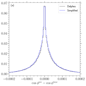
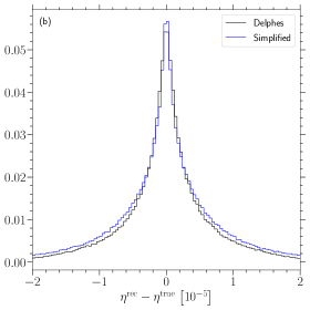
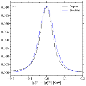
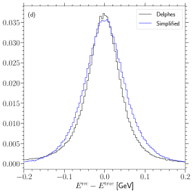
Fig. 2: The pion smearing effects simulated by Delphes (black) and our simplified algorithm (blue). Notice that in the panel $(b)$ the numbers in the horizontal axis are multiplied by a factor $\times 10^{5}$ for better visualization.

Although our simplified smearing algorithm is admittedly less sophisticated, our results are broadly compatible with those commonly adopted in the literature. A complete analysis in momentum reconstruction and detailed cuts was performed in Refs. [50, 41]. For validation, we compare our smearing algorithm to the Delphes simulation with the configurations cards delphes_card_CircularEE.tcl [51] for the CEPC/FCC-ee [54] and delphes_card_ILD.tcl [52] for the ILC. Fig. 2 shows the smeared distributions of the pion kinematic variables simulated with Delphes (black) vs our simplified smearing (blue). We can see that the results of these two simulations agree with each other quite well. In this work, we take the simplified smearing algorithm for a fast simulation.

To obtain the total number of expected events, one needs to consider several branching ratios. First, the $Z$ boson can only be reconstructed if it decays into either leptons or jets with $80\%$ of branching ratio in total [44]. Also, since the decay branching ratio of Higgs decaying into two $\tau$ leptons is $6.64\%$ [44], only around 5.3% of the actual Higgs events associated with $Z$ production are available for the CP measurement. Further suppression comes from the branching fraction of the decay of $\tau$ into $\pi$ or $\rho$. And we arrive at 7704 events at the CEPC, 7003 events at the FCC-ee, and 4482 events at the ILC. Taking into account the identification of $\tau$ jets and tagging of the Higgs boson and other selection cuts [40], we obtain an overall efficiency, $\epsilon=0.145,0.144,0.142$ for $(\pi,\pi),(\pi,\rho)$ and $(\rho,\rho)$ decay modes, respectively.

Decay modes	Branching ratio
$Z\rightarrow$ vis.	80%
$h\rightarrow\tau^{+}\tau^{-}$	6.64%
$\tau\rightarrow\pi\nu_{\tau}$	10.82%
$\tau\rightarrow\rho\nu_{\tau}$	25.49%

$\tau$ decay products	Number of Higgs decay events
	CEPC		FCC-ee		ILC
	before	after	before	after	before	after
$(\pi,\pi)$	684	99	622	90	398	58
$(\pi,\rho)$	3223	465	2930	423	1875	271
$(\rho,\rho)$	3797	541	3451	491	2209	314

Table 3: Left: Branching fractions associated with the entire reaction. The values were obtained from [44]. Right: Expected event numbers at the CEPC [7] with the integrated luminosity $\mathcal{L}=5.6~{}$ab^-1, FCC-ee [8] with $\mathcal{L}=5~{}$ab^-1 and ILC [46] with $\mathcal{L}=2~{}$ab^-1. The expected numbers of events before and after selection cuts are shown in the columns “before” and “after”, respectively, with the overall cut efficiencies taken from Ref. [40].

The expected event numbers before and after applying the selection efficiencies are shown in Table 3 for comparison. In total, roughly 1105, 1004, and 643 events of the $h\to\tau^{+}\tau^{-},\tau^{\pm}\to\pi^{\pm}/\rho^{\pm}\nu_{\tau^{\pm}}$ decay chains can be reconstructed at the CEPC, FCC-ee, and ILC, respectively.

3.2 Ambiguities in Momentum Reconstruction

Experimentally, in order to reconstruct the $\tau$ momentum, it is unavoidable to first obtain the neutrino momentum which is not directly detectable. With two neutrinos in the final state, we need to constrain two 4-vector momenta. Since the Higgs momentum can be fully reconstructed from the $Z$ boson counterpart, only one neutrino momentum is independent due to energy-momentum conservation. The 4 degrees of freedom can be constrained by the on-shell conditions of the two neutrinos and the two $\tau$ leptons.

Unfortunately, the solutions have a two-fold ambiguity. Since on-shell conditions are in quadratic forms, one sign can not be uniquely fixed. For completeness, we summarize the solution here in terms of the $\tau^{-}$ momentum defined in the Higgs rest frame,

$${\bf p}_{\tau_{-}} = \sqrt{p^{2}_{h}-4m^{2}_{\tau}}\left[\sin\theta_{\tau}\left(\cos\phi_{\tau}{\hat{\bf n}}_{1}+\sin\phi_{\tau}{\hat{\bf n}}_{2}\right)\pm\cos\theta_{\tau}{\hat{\bf n}}_{3}\right].$$ (3.2)

The unit base vectors $\hat{\bf n}_{i}$ are constructed in terms of the primary decay mesons, $X_{\pm}\equiv\pi^{\pm},\rho^{\pm}$,

$${\hat{\bf n}}_{1}={\hat{\bf p}}_{X_{+}}\,,\quad{\hat{\bf n}}_{2}=\frac{{\hat{\bf p}}_{X_{-}}-({\hat{\bf p}}_{X_{+}}\cdot{\hat{\bf p}}_{X_{-}}){\hat{\bf p}}_{X_{+}}}{\sqrt{1-({\hat{\bf p}}_{X_{+}}\cdot{\hat{\bf p}}_{X_{-}})^{2}}},\qquad{\hat{\bf n}}_{3}=\frac{{\hat{\bf p}}_{X_{+}}\times{\hat{\bf p}}_{X_{-}}}{\sqrt{1-({\hat{\bf p}}_{X_{+}}\cdot{\hat{\bf p}}_{X_{-}})^{2}}}\,.$$ (3.3)

The first base vector $\hat{\bf n}_{1}$ is along the momentum of $\pi^{+}$ or $\rho^{+}$ while the third one $\hat{\bf n}_{3}$ is perpendicular to the momentum of both primary mesons. Finally, $\hat{\bf n}_{2}$ is simply the one perpendicular to both $\hat{\bf n}_{1}$ and $\hat{\bf n}_{3}$. The polar angles of the $\tau$ momentum can be reconstructed as,

$$\sin\theta_{\tau}\cos\phi_{\tau} = \frac{m^{2}_{\tau}+m^{2}_{X}-m_{h}E_{X_{+}}}{|{\bf p}_{X_{+}}|\sqrt{m^{2}_{h}-4m^{2}_{\tau}}},$$ (3.4a)

$$\sin\theta_{\tau}\sin\phi_{\tau} = \frac{m_{h}E_{X_{-}}-m^{2}_{\tau}-m^{2}_{X_{-}}}{|{\bf p}_{X_{-}}||s_{X_{-}X_{+}}|\sqrt{m^{2}_{h}-4m^{2}_{\tau}}}+\frac{m_{h}E_{X_{+}}-m^{2}_{\tau}-m^{2}_{X_{+}}}{|{\bf p}_{X_{+}}||s_{X_{-}X_{+}}|\sqrt{m^{2}_{h}-4m^{2}_{\tau}}}c_{X_{-}X_{+}}\;,\qquad$$ (3.4b)

where $(s_{X_{-}X_{+}},c_{X_{-}X_{+}})\equiv(\sin\theta_{X_{-}X_{+}},\cos\theta_{X_{-}X_{+}})$ and $\theta_{X_{-}X_{+}}$ is the angle between the momentum of $X_{+}$ and $X_{-}$.

However, in Eq. (3.2) the $\pm$ sign in front of $\hat{\bf n}_{3}$ reflects the fact that both solutions obey all the constraints from energy-momentum conservation and the correct solution cannot be unambiguously obtained. This sign ambiguity can significantly decrease the CP sensitivity, especially for the neutrino azimuthal angle distribution. Using momentum conservation, the result in Eq. (2.7) for $\tan\delta\phi_{\nu}$ can be written in the same form by substituting ${\bf p}_{\nu}$ by ${\bf p}_{X^{\pm}}$, hence, $\tan\delta\phi_{\nu}\propto{\hat{\bf p}}_{\tau^{-}}\cdot({\bf p}_{X^{+}}\times{\bf p}_{X^{-}})=\pm\cos\theta_{\tau}/\sqrt{1-({\hat{\bf p}}_{X_{+}}\cdot{\hat{\bf p}}_{X_{-}})^{2}}$. In other words, $\delta\phi_{\nu}$ can have both positive and negative solutions with the same magnitude. This would not be a big problem for the symmetric distribution of $\delta\phi_{\nu}$ around its origin, such as those curves in Fig. 1 with $\Delta=0^{\circ}$. But it causes significant issues for other $\Delta$ values and effectively flattens the curve for $\Delta=\pm 45^{\circ}$.

This ambiguity can be solved by measuring other decay information. An especially useful quantity is the impact parameter [55, 56], the minimum distance of charged meson trajectory to the $\tau$ leptons production point. The impact parameter measurement essentially removes the two-fold ambiguity for the $\tau$ Yukawa CP measurement at future lepton colliders [24, 53]. A more recent study with spatial resolution of 5 $\mu$m can be found in Refs. [41, 40].

Another ambiguity comes from the detector resolutions. The $\tau$ momentum is reconstructed from the smeared Higgs and meson momentum. This reconstruction is realized with energy and momentum conservation, assuming narrow width approximation for the $\tau$ momentum, $p_{\tau^{\pm}}^{2}=m_{\tau}^{2}$. Both smearing and finite width could lead to nonphysical solutions in Eq. (3.4), for example $\sin\theta_{\tau}\sin\phi_{\tau}>1$. For those events, we follow a similar procedure introduced in Ref. [41]. We try to find the solution for the (anti-)neutrino momenta optimally consistent with all the information we have on each event (including four-momentum conservation) by minimizing the function

$$\chi^{2}_{\rm rec}=\sum_{i=0}^{3}\left(\frac{(p^{\rm rec}_{\tau^{+}})_{i}+(p^{\rm rec}_{\tau^{-}})_{i}-(p^{\rm rec}_{h})_{i}}{\sigma_{h}}\right)^{2}+\left(\frac{(p^{\rm rec}_{\tau^{+}})^{2}-m_{\tau}^{2}}{\sigma_{\tau}}\right)^{2}+\left(\frac{(p^{\rm rec}_{\tau^{-}})^{2}-m_{\tau}^{2}}{\sigma_{\tau}}\right)^{2},$$ (3.5)

where $i=0,\cdots,3$ runs over the 4-momentum components of each particle momentum. We adopt the uncertainties as $\sigma_{h}=4.0$ GeV and $\sigma_{\tau}=0.2$ GeV [41]. The $\chi^{2}_{\rm rec}$ function is minimized over the 6 kinematic parameters of the unmeasured neutrino momentum: the pseudo-rapidity, azimuthal angle, and absolute value of the momentum for both neutrino/anti-neutrino. Then the $\tau$ momentum is then obtained with energy momentum conservation, $p^{\rm rec}_{\tau^{\pm}}=p_{\nu^{\pm}}+p^{\rm rec}_{X^{\pm}}$. The best fit at the minimum of $\chi^{2}_{\rm rec}$ approximates the physical solution. We keep the event if the minimum solution is consistent with the mass cuts. Otherwise, the event is discarded.

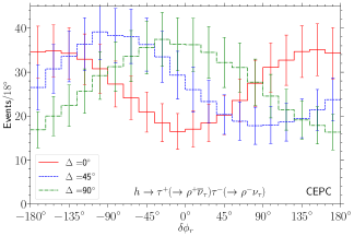
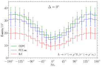
Fig. 3: Smeared differential distributions of $\delta\phi_{r}$ in the decay mode $h\rightarrow\tau^{+}(\rightarrow\rho^{+}\overline{\nu}_{\tau})\tau^{-}(\rightarrow\rho^{-}\nu_{\tau})$. Left: The distribution for CP phases $\Delta=0^{\circ}$ (red), $\Delta=45^{\circ}$ (blue), $\Delta=90^{\circ}$ (green) at the CEPC; Right: A comparison of the distributions at the CEPC (red), FCC-ee (blue), and ILC (green) for $\Delta=0^{\circ}$. In both panels, the error bars indicate the statistical uncertainties.

The final result of the differential distribution for the $h\rightarrow\tau^{+}(\rightarrow\rho^{+}\overline{\nu}_{\tau})\tau^{-}(\rightarrow\rho^{-}\nu_{\tau})$ process is plotted in Fig. 3. The left panel shows the differential distributions for $\Delta=0^{\circ}$ (red), $\Delta=45^{\circ}$ (blue), and $\Delta=90^{\circ}$ (green), respectively. Being divided into 20 bins [33, 40], there are $25\sim 35$ events in each bin on average. The corresponding statistical uncertainty at the level of $17\%\sim 20\%$ is much smaller than the oscillation amplitude, $\pi^{2}/16\approx 62\%$. The event rate at the CEPC are large enough to constrain the modulation pattern as elaborated in Sec. 3.3. The right panel shows the spectrum at the three future candidate lepton colliders, CEPC (red), FCC-ee (blue), and ILC (green), respectively, for comparison. While CEPC and FCC-ee have comparable spectrum, ILC has much lower event rate and hence larger fluctuations.

It is interesting to see that for $\Delta=90^{\circ}$, the differential distribution of $\delta\phi_{r}$ has only $\cos\delta\phi_{r}$ but no $\sin\delta\phi_{r}$ in Eq. (2.6). In other words, the observable that we measure has only CP conserving contribution that does not change under CP transformation. However, the distributions in the left panel of Fig. 3 show that the difference between $\Delta=0^{\circ}$ and $\Delta=90^{\circ}$ is maximal. This is because $\cos 2\Delta=\pm 1$ take the two extreme values with opposite signs.

3.3 Discovery Potential and Sensitivity of the CP Phase

To evaluate the CP measurement sensitivities, we adopt a $\chi^{2}$ function defined according to the Poisson distribution,

$$\chi^{2}\equiv\sum_{i}2(N_{i}^{\rm test}-N_{i}^{\rm true})+2N_{i}^{\rm true}\log(N_{i}^{\rm true}/N_{i}^{\rm test}),$$ (3.6)

where $i=1,\cdots,20$ runs over all the 20 bins of the $\delta\phi_{r}$ differential distribution. Since we are studying the projected sensitivity at future lepton colliders, there is no real data available yet. Instead, we simulate the measurement with some assumed true values of the CP phase $\Delta$ to produce a set of pseudo-data $N^{\rm true}_{i}$ and then fit these pseudo-data with some test values $N^{\rm test}_{i}$. The event numbers $N^{\rm true}_{i}$ and $N^{\rm test}_{i}$ are functions of the true value $\Delta^{\rm true}$ and $\Delta^{\rm test}$, respectively.

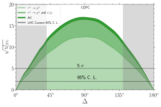
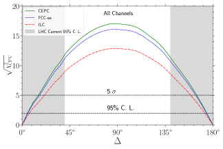
Fig. 4: Left: The CP phase discovery potential at the CEPC for $\kappa_{\tau}=1$. The green shaded regions represent the results from various decay modes: only $(\rho,\rho)$ (light green), $(\rho,\rho)+(\pi,\rho)$ (green) and the fully combined one $(\rho,\rho)+(\pi,\rho)+(\pi,\pi)$ (dark green), with the boundaries describing the $\sqrt{\chi^{2}_{\rm CPV}}$ values according to Eq. (3.7) given $\Delta^{\rm{true}}$. The black dashed lines with $\sqrt{\chi_{\rm{CPV}}^{2}}=1.96,5$ mark the sensitivities at $95\%$ C.L. and $5\sigma$, respectively. Right: Sensitivity of all the channels at the CEPC (green), FCC-ee (blue), and ILC (red). In both panels, the region outside of the gray bands are excluded at 95% C.L. by the current CP measurement at the LHC [42].

The discovery ability of a nonzero CP phase can be parametrized as the smaller one of the two $\chi^{2}$ values between the given $\Delta^{\rm true}$ and the CP conserving cases $\Delta^{\rm test}=0^{\circ}$ or $\Delta^{\rm test}=180^{\circ}$,

$$\chi^{2}_{\rm CPV}(\Delta^{\rm true})\equiv{\rm min}[\chi^{2}(\Delta^{\rm true},\Delta^{\rm test}=0^{\circ}),\chi^{2}(\Delta^{\rm true},\Delta^{\rm test}=180^{\circ})].$$ (3.7)

Fig. 4 shows the $\sqrt{\chi^{2}_{\rm CPV}}$ distribution as a function of $\Delta$ assuming $\kappa_{\tau}=1$. The sensitivities for the di-$\tau$ decay into $(\rho,\rho)$, $(\rho,\rho)+(\pi,\rho)$, and the full combination $(\rho,\rho)+(\pi,\rho)+(\pi,\pi)$ are depicted in light green, green, and dark green regions, respectively. For different decay channels, the differential distributions have the same amplitude $\pi^{2}/16$ as indicated in Eq. (2.6). So the main difference in the sensitivities is due to the event rates: the branching ratio of the $\tau\rightarrow\pi\nu_{\tau}$ is only $10.8\%$, in comparison with the $25\%$ for the $\tau\rightarrow\rho\nu_{\tau}$ channel. As indicated by the black dashed lines, 95% of the values of $\Delta$ can be tested above $95\%$ C.L. and 82% of the parameter space can be tested at even more than $5\sigma$. The sensitivity peaks at $\Delta=\pm 90^{\circ}$ where Eq. (2.6) takes the most different value from that of $\Delta=0^{\circ}$ or $180^{\circ}$ with more than $10\,\sigma$ significance. In the right panel, we also show the comparison of the sensitivities at the CEPC (green), FCC-ee (blue), and ILC (red). As expected, the CEPC has the highest sensitivity due to the higher number of events.

	68% C.L. for $m=1$	95% C.L. for $m=1$	95% C.L. for $m=2$
CEPC	2.9∘	5.6∘	7.0∘
FCC-ee	3.2∘	6.3∘	7.8∘
ILC	3.8∘	7.4∘	9.3∘

Table 4: The CP phase precision at the CEPC, FCC-ee, and ILC for $m$ parameter(s)

.

For completeness, Table 4 summarizes the expected precision of the $\Delta$ measurement at future lepton colliders at 68% C.L. and 95% C.L. for $m=1$ parameter ($\Delta$), or $m=2$ parameters ($\Delta$ and $\kappa_{\tau}$). Notice that our estimation at $1\,\sigma$ level is slightly better than the $4.4^{\circ}$ with $1\,\mbox{ab}^{-1}$ in only the $\tau\rightarrow\rho\nu_{\tau}$ decay channel [33] or $4.3^{\circ}$ with $2\,\mbox{ab}^{-1}$ in both $\tau$ decay channels [40] at the ILC. For the CEPC, our result is the same as the $2.9^{\circ}$ in Ref. [41]. Notice that in addition to the two mesonic decay channels, the leptonic decay channel $\tau\rightarrow\ell\nu\bar{\nu}$ is also considered in Ref. [41] with the matrix element based observable that is different from our polarimeter $\delta\phi_{r}$. We can clearly see from Table 4 that the future lepton colliders can differentiate the CPV scenario from the CP-conserving one very well.

4 Prospects of Constraining New Physics

As the aforementioned analysis shows, there remains significant potential for discovering CP violation in the $h\to\tau^{+}\tau^{-}$ decay at prospective future lepton colliders. We now draw the connection with the lepton flavored EWBG scenario, following the treatment given in Ref. [14] for concrete illustration (see Refs.[15, 16, 17, 18]).This discussion exemplifies future lepton colliders are not only precision machines but can also make an $\mathcal{O}(1)$ measurement of BSM physics effects.

4.1 Two Higgs Doublet Model

The set up in Ref. [14] relies on the type III Two Higgs Doublet Model (THDM) [57, 58], wherein the two scalar doublet fields before EWSB are denoted as $\Phi_{1,2}$. Both neutral scalars inside $\Phi_{1,2}$ acquire nonzero VEVs, $v_{1}$ and $v_{2}$, respectively, with $v\equiv\sqrt{v_{1}^{2}+v_{2}^{2}}=246$ GeV. The neutral components can mix with each other to form three neutral massive scalar fields after one neutral Goldstone boson is eaten by the $Z$ boson. We assume a CP-invariant scalar potential, namely, only the real parts of the two neutral scalars can mix with each other but not with the imaginary parts,

$$H\equiv c_{\alpha}{\rm Re}[\Phi^{0}_{1}]+s_{\alpha}{\rm Re}[\Phi^{0}_{2}],\quad h\equiv-s_{\alpha}{\rm Re}[\Phi^{0}_{1}]+c_{\alpha}{\rm Re}[\Phi^{0}_{2}],\quad A\equiv-s_{\beta}{\rm Im}[\phi_{1}^{0}]+c_{\beta}{\rm Im}[\phi_{2}^{0}],$$ (4.1)

where $s_{\alpha}\equiv\sin\alpha$, $c_{\alpha}\equiv\cos\alpha$, $\tan\beta\equiv v_{2}/v_{1}$, and Re and Im denote the real and imaginary parts, respectively. Note that $\alpha$ is the mixing angle from the neutral scalar mass matrix diagonalization. The neutral particle masses are ordered as $m_{H},m_{A}>m_{h}\approx 125$ GeV, so that $h$ is the SM-like Higgs boson.

In the Type-III THDM, the Yukawa interaction for each doublet field has the same structure as the SM Yukawa interaction;

$$\mathcal{L}_{Y}=-\overline{L}Y_{1}\ell_{R}\Phi_{1}-\overline{L}Y_{2}\ell_{R}\Phi_{2}+{\rm h.c.}$$ (4.2)

In this way, both Higgs doublets can contribute its neutral components to couple with the $\tau$ lepton [29],

$$-\frac{m_{\tau}}{v}\overline{\tau}_{L}\tau_{R}\left[\left(s_{\beta-\alpha}+\frac{N_{\tau\tau}}{m_{\tau}}c_{\beta-\alpha}\right)h+\left(c_{\beta-\alpha}-\frac{N_{\tau\tau}}{m_{\tau}}s_{\beta-\alpha}\right)H+iAN_{\tau\tau}\right],$$ (4.3)

where $N_{\tau\tau}$ is a complex parameter related to the matrix elements of $Y_{1,2}$. Following the parametrization of Eq. (2.1), the $\tau$ Yukawa coupling becomes

$$\kappa_{\tau}(\cos\Delta+i\sin\Delta)=s_{\beta-\alpha}+\frac{N_{\tau\tau}}{m_{\tau}}c_{\beta-\alpha}.$$ (4.4)

Notice that CP violation arises due to the imaginary part of $N_{\tau\tau}$. Moreover, for the particular texture, $Y_{j,22}=Y_{j,23}=0$, $Y_{1,33}=Y_{2,33}=Y_{33}$ and $Y_{1,32}=r_{32}Y_{2,32}$, one can write the imaginary part of the Jarskog invariant $J_{A}$ of the Yukawa interaction in Eq. (4.2) as,

$$\mathrm{Im}[J_{A}]=-\mathrm{Im}[r_{32}]|Y_{2,32}|^{2}=\frac{2m^{2}_{\tau}}{v^{2}c_{\beta-\alpha}}\kappa_{\tau}\sin\Delta\,.$$ (4.5)

It is the imaginary part of the Jarlskog invariant that controls the size of the BAU in early universe through lepton flavored baryogenesis [14]. Rewriting Eq. (4.5) gives

$$\sin\Delta=\frac{v^{2}c_{\beta-\alpha}}{2m^{2}_{\tau}\kappa_{\tau}}\mathrm{Im}[J_{A}].$$ (4.6)

Thus, one may connect the $\tau$ Yukawa CP phase $\Delta$, which can be measured at future lepton colliders, with CPV source for baryogenesis during the era of EWSB in the early universe.

4.2 Sensitivity to the Baryogenesis Scenario

To make this connection concrete, we plot in Fig. 5 the 95% C.L. constraints on $\kappa_{\tau}\cos\Delta$ and $\kappa_{\tau}\sin\Delta$ from present and future collider probes and from lepton flavored EWBG. For generality, we also set $\kappa_{\tau}^{\rm test}$ to be free to obtain a full picture on a two-dimensional plot. The CP sensitivity is then depicted as the contours around the true value $\Delta^{\rm true}=0^{\circ}$ and $\kappa^{\rm true}_{\tau}=1$ in the left pannel, with the green, blue (dashed), and red (dot dashed) contours indicating the 95% C.L. sensitivities. The green dotted lines from the origin $\kappa_{\tau}=0$ are added to show that the contour size corresponds to roughly $7^{\circ}$ at 95% C.L. Consistent with the previous observation, the CEPC and FCC-ee have comparable precision while that of the ILC is slightly weaker due to different luminosities. For all three cases, the pink region allowing for successful explanation of BAU is outside the 95% C.L. contour. In other words, the lepton flavored BAU mechanism as given in Ref. [14] could be excluded at better than than 95% C.L. . For comparison, we also show the projected $\tau$ Yukawa CP measurement at the High Luminosity (HL-)LHC [38] with the integrated luminosity of $3\,\mbox{ab}^{-1}$ as the black contour, which will be further elaborated below. It is clear that even with the HL-LHC, the THDM BAU mechanism can only be tested with barely 95% C.L. The CP measurements at future lepton colliders can significantly improve the situation.

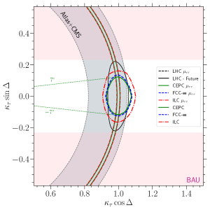
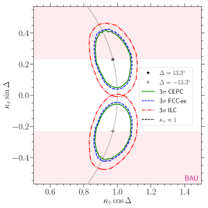
Fig. 5: Left: The 95% C.L. constraints on the $\tau$ Yukawa coupling at the CEPC (green), FCC-ee (blue), and ILC (red) assuming the true value $\Delta^{\rm true}=0^{\circ}$ and $\kappa^{\rm true}_{\tau}=1$. The gray band gives 95% C.L. constraints from the current LHC signal strength measurements [5, 6] while the black contour denotes the expected 95% C.L. constraint from the combined measurements of $\mu_{\tau\tau}$ [59, 60] and $\Delta$ [38] at the HL-LHC. Right: The 3$\sigma$ contours for each collider assuming central values $\Delta^{\rm true}=\pm 13.3^{\circ}$ and $\kappa^{\rm true}_{\tau}=1$ corresponding to the minimum $|\kappa_{\tau}\sin\Delta|$ compatible with the BAU.

We also include the constraints from the measurement of the $h\to\tau\tau$ decay signal strength $\mu_{\tau\tau}$, which is proportional to $\kappa_{\tau}^{2}$. The current data at the LHC indicate $\mu_{\tau\tau}=1.09^{+0.35}_{-0.30}$ at ATLAS [5] and $\mu_{\tau\tau}=0.85^{+0.12}_{-0.11}$ at CMS [6], which are depicted as the gray region. In other words, the current measurement at LHC is still quite crude with at least 10% uncertainty. At the HL-LHC, the $1\,\sigma$ uncertainty of $\mu_{\tau\tau}$ can be further improved to $5\%$ [59, 60], which is further combined with the CP measurement [38] that is shown as the black contour. The future lepton colliders can significantly improve the sensitivities to 0.8% at the CEPC [61], 0.9% at the FCC-ee [8], and 1.09% at the ILC [61], which are shown as the rings in the left panel of Fig. 5. Note that these rings with inclusive $\tau$ decays are much narrower than the width of the contours or equivalently the marginalized sensitivity on $\kappa_{\tau}$ after integrating out the CP phase $\Delta$ from the original two-dimensional distributions. The discrepancy comes from the fact that the $\tau\rightarrow\pi\nu_{\tau}$ and $\tau\rightarrow\rho\nu_{\tau}$ channels contribute only a very small fraction ($\sim 13\%$) of the inclusive decay events. The strength measurement can provide very important complementary info and reduce the parameter space to be explored.

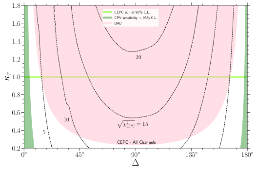
Fig. 6: The CP discovery capability of the CEPC as a function of the $\Delta$ and $\kappa_{\tau}$ true values. The black dashed lines represents several typical values of the significance, $\sqrt{\chi^{2}_{\rm CPV}}=5,10,15,20$. The green region represents the space parameter where the sensitivity is below 95% C.L. The pink region represents the parameter space that can explain the BAU in the lepton flavored EWBG scenario [14].

Instead of assuming the SM values $\kappa^{\rm true}_{\tau}=1$ and $\Delta^{\rm true}=0^{\circ}$, it is interesting to ask the whether the lepton flavored EWBG scenario can explain the BAU and at the same time produce a signal that is distinguishable from the SM. To address this question, we show in the right panel of Fig. 5 the similar contours around $\Delta^{\rm true}=\pm 13.3^{\circ}$ and $\kappa^{\rm true}_{\tau}=1$ that is at the boundary of the BAU region. Under this assumption, the CEPC and FCC could establish the presence of CPV in the $\tau$ Yukawa interaction with $3\sigma$ significance, while for the ILC the significance would be somewhat weaker.

It is also interesting to investigate the behavior of the CP violation sensitivity when one varies the assumed true values of $\kappa_{\tau}$. This can be observed from Fig. 6 where we show the sensitivity as a function of the CP phase $\Delta$ and the coupling strength $\kappa_{\tau}$. The dashed gray lines give several typical sensitivities $\sqrt{\chi^{2}_{\rm CPV}}=5,10,15,20$. Note that the dashed gray lines expand with larger $\tau$ Yukawa coupling due to event number enhancement. This is especially significant for small $\kappa_{\tau}$ while for large values of $\kappa_{\tau}$ the CP sensitivity does not change substantially. The BAU-compatible region has a lower limit at $\kappa_{\tau}\approx 0.25$ due to the lower limit on $\kappa_{\tau}\sin\Delta$ according to Fig. 5 and most of the BAU-compatible region falls inside the $\sqrt{\chi^{2}_{\rm CPV}}=5$ curve, corresponding to $5\,\sigma$ discovery.

5 Conclusions

Explaining the origin of the baryon asymmetry of the Universe is a key open problem at the interface of particle and nuclear physics with cosmology. An essential ingredient in the explanation is the presence of BSM CP violation. In the electroweak baryogenesis scenario, the relevant CPV interactions would have generated the BAU during the era of EWSB. The corresponding mass scale makes these interactions in principle experimentally accessible. While null results for permanent EDM searches place strong constraints on new flavor diagonal, electroweak scale CPV interactions, flavor changing CPV effects are significantly less restricted. Lepton flavored EWBG draws on this possibility, with interesting implications for CPV in the tau-lepton Yukawa sector.

In this work, we have shown how measurements of CPV observable in Higgs di-tau decays at prospective future lepton colliders could test this possibility, with significant discovery potential if it is realized in nature. After making a detailed comparison of the four differential distributions of the neutrino azimuth angle $\delta\phi_{\nu}$, polarimeter $\delta\phi_{r}$, acoplanarity $\phi^{*}$, and the $\Theta$ variable for the first time as well as various detector responses, we explore the prospects of CP measurement in the $\tau$ Yukawa coupling at future lepton colliders. With $(5.6,5,2)\,\mbox{ab}^{-1}$ luminosity, the $1\,\sigma$ uncertainty can reach $2.9^{\circ},3.2^{\circ},3.8^{\circ}$ at the CEPC, FCC-ee, and ILC, respectively. This allows the possibility of distinguishing the attainable EWBG from the CP conserving case with $3\,\sigma$ sensitivity. The future lepton colliders are not just precision machines for detailing our understanding of the Higgs boson, but can also make $\mathcal{O}(1)$ measurement of the possible new physics beyond the SM.

References

- [1] G. Aad et al. [ATLAS], “Observation of a new particle in the search for the Standard Model Higgs boson with the ATLAS detector at the LHC,” Phys. Lett. B 716 (2012), 1-29 [arXiv:1207.7214 [hep-ex]].
- [2] S. Chatrchyan et al. [CMS], “Observation of a New Boson at a Mass of 125 GeV with the CMS Experiment at the LHC,” Phys. Lett. B 716 (2012), 30-61 [arXiv:1207.7235 [hep-ex]].
- [3] S. Chatrchyan et al. [CMS], “Evidence for the 125 GeV Higgs boson decaying to a pair of leptons,” JHEP 05, 104 (2014) [arXiv:1401.5041 [hep-ex]].
- [4] G. Aad et al. [ATLAS], “Evidence for the Higgs-boson Yukawa coupling to tau leptons with the ATLAS detector,” JHEP 04, 117 (2015) [arXiv:1501.04943 [hep-ex]].
- [5] M. Aaboud et al. [ATLAS], “Cross-section measurements of the Higgs boson decaying into a pair of -leptons in proton-proton collisions at TeV with the ATLAS detector,” Phys. Rev. D 99, 072001 (2019) [arXiv:1811.08856 [hep-ex]].
- [6] [CMS Collaboration], “Measurement of Higgs boson production in the decay channel with a pair of leptons,” CMS-PAS-HIG-19-010.
- [7] J. B. Guimarães da Costa et al. [CEPC Study Group], “CEPC Conceptual Design Report: Volume 2 - Physics & Detector,” [arXiv:1811.10545 [hep-ex]].
- [8] A. Abada et al. [FCC], “FCC-ee: The Lepton Collider: Future Circular Collider Conceptual Design Report Volume 2,” Eur. Phys. J. ST 228, no.2, 261-623 (2019)
- [9] H. Baer, T. Barklow, K. Fujii, Y. Gao, A. Hoang, S. Kanemura, J. List, H. E. Logan, A. Nomerotski and M. Perelstein, et al. “The International Linear Collider Technical Design Report - Volume 2: Physics,” [arXiv:1306.6352 [hep-ph]].
- [10] A. D. Sakharov, “Violation of CP Invariance, C asymmetry, and baryon asymmetry of the universe,” Sov. Phys. Usp. 34 (1991) no.5, 392-393
- [11] D. E. Morrissey and M. J. Ramsey-Musolf, “Electroweak baryogenesis,” New J. Phys. 14 (2012), 125003 [arXiv:1206.2942 [hep-ph]].
- [12] J. Engel, M. J. Ramsey-Musolf and U. van Kolck, “Electric Dipole Moments of Nucleons, Nuclei, and Atoms: The Standard Model and Beyond,” Prog. Part. Nucl. Phys. 71, 21-74 (2013) [arXiv:1303.2371 [nucl-th]].
- [13] T. Chupp, P. Fierlinger, M. Ramsey-Musolf and J. Singh, “Electric dipole moments of atoms, molecules, nuclei, and particles,” Rev. Mod. Phys. 91 (2019) no.1, 015001 [arXiv:1710.02504 [physics.atom-ph]].
- [14] H. K. Guo, Y. Y. Li, T. Liu, M. Ramsey-Musolf and J. Shu, “Lepton-Flavored Electroweak Baryogenesis,” Phys. Rev. D 96, no.11, 115034 (2017) [arXiv:1609.09849 [hep-ph]].
- [15] C. W. Chiang, K. Fuyuto and E. Senaha, “Electroweak Baryogenesis with Lepton Flavor Violation,” Phys. Lett. B 762, 315-320 (2016) [arXiv:1607.07316 [hep-ph]].
- [16] J. De Vries, M. Postma and J. van de Vis, “The role of leptons in electroweak baryogenesis,” JHEP 04, 024 (2019) [arXiv:1811.11104 [hep-ph]].
- [17] E. Fuchs, M. Losada, Y. Nir and Y. Viernik, “ violation from , and dimension-6 Yukawa couplings - interplay of baryogenesis, EDM and Higgs physics,” JHEP 05, 056 (2020) [arXiv:2003.00099 [hep-ph]].
- [18] K. P. Xie, “Lepton-mediated electroweak baryogenesis, gravitational waves and the final state at the collider,” [arXiv:2011.04821 [hep-ph]].
- [19] M. J. Ramsey-Musolf, “The electroweak phase transition: a collider target,” JHEP 09, 179 (2020) [arXiv:1912.07189 [hep-ph]].
- [20] J. R. Dell’Aquila and C. A. Nelson, “Usage of the or T Anti-t Decay Mode to Distinguish an Intermediate Mass Higgs Boson From a Technipion,” Nucl. Phys. B 320 (1989), 86-102.
- [21] J. R. Dell’Aquila and C. A. Nelson, “{CP} Determination for New Spin Zero Mesons by the Decay Mode,” Nucl. Phys. B 320, 61-85 (1989).
- [22] G.gR. Bower, T. Pierzchala, Z. Was and M. Worek, “Measuring the Higgs boson’s parity using tau — rho nu,” Phys. Lett. B 543, 227-234 (2002) [arXiv:hep-ph/0204292 [hep-ph]].
- [23] M. Worek, “Higgs CP from H / A0 tau tau decay,” Acta Phys. Polon. B 34 (2003), 4549-4560 [arXiv:hep-ph/0305082 [hep-ph]].
- [24] K. Desch, Z. Was and M. Worek, “Measuring the Higgs boson parity at a linear collider using the tau impact parameter and tau — rho nu decay,” Eur. Phys. J. C 29, 491-496 (2003) [arXiv:hep-ph/0302046 [hep-ph]].
- [25] K. Desch, A. Imhof, Z. Was and M. Worek, “Probing the CP nature of the Higgs boson at linear colliders with tau spin correlations: The Case of mixed scalar - pseudoscalar couplings,” Phys. Lett. B 579, 157-164 (2004) [arXiv:hep-ph/0307331 [hep-ph]].
- [26] S. Berge and W. Bernreuther, “Determining the CP parity of Higgs bosons at the LHC in the tau to 1-prong decay channels,” Phys. Lett. B 671, 470-476 (2009) [arXiv:0812.1910 [hep-ph]].
- [27] S. Berge, W. Bernreuther and J. Ziethe, “Determining the CP parity of Higgs bosons at the LHC in their tau decay channels” Phys. Rev. Lett. 100, 171605 (2008) [arXiv:0801.2297 [hep-ph]].
- [28] S. Berge, W. Bernreuther, B. Niepelt and H. Spiesberger, “How to pin down the CP quantum numbers of a Higgs boson in its tau decays at the LHC,” Phys. Rev. D 84 (2011), 116003 [arXiv:1108.0670 [hep-ph]].
- [29] S. Berge, W. Bernreuther and S. Kirchner, “Prospects of constraining the Higgs boson’s CP nature in the tau decay channel at the LHC,” Phys. Rev. D 92 (2015), 096012 [arXiv:1510.03850 [hep-ph]].
- [30] J. R. Ellis, J. S. Lee and A. Pilaftsis, “CERN LHC signatures of resonant CP violation in a minimal supersymmetric Higgs sector,” Phys. Rev. D 70, 075010 (2004) [arXiv:hep-ph/0404167 [hep-ph]].
- [31] S. Berge, W. Bernreuther and H. Spiesberger, “Higgs CP properties using the decay modes at the ILC,” Phys. Lett. B 727, 488-495 (2013) [arXiv:1308.2674 [hep-ph]].
- [32] B. Grzadkowski and J. F. Gunion, “Using decay angle correlations to detect CP violation in the neutral Higgs sector,” Phys. Lett. B 350, 218-224 (1995) [arXiv:hep-ph/9501339 [hep-ph]].
- [33] R. Harnik, A. Martin, T. Okui, R. Primulando and F. Yu, “Measuring CP Violation in at Colliders,” Phys. Rev. D 88 (2013) no.7, 076009 [arXiv:1308.1094 [hep-ph]].
- [34] A. Askew, P. Jaiswal, T. Okui, H. B. Prosper and N. Sato, “Prospect for measuring the CP phase in the coupling at the LHC,” Phys. Rev. D 91, no.7, 075014 (2015) [arXiv:1501.03156 [hep-ph]].
- [35] K. Hagiwara, K. Ma and S. Mori, “Probing CP violation in at the LHC,” Phys. Rev. Lett. 118 (2017) no.17, 171802 [arXiv:1609.00943 [hep-ph]].
- [36] A. Bhardwaj, P. Konar, P. Sharma and A. K. Swain, “Exploring CP phase in -lepton Yukawa coupling in Higgs decays at the LHC,” J. Phys. G 46 (2019) no.10, 105001 [arXiv:1612.01417 [hep-ph]].
- [37] T. Han, S. Mukhopadhyay, B. Mukhopadhyaya and Y. Wu, “Measuring the CP property of Higgs coupling to tau leptons in the VBF channel at the LHC,” JHEP 05, 128 (2017) [arXiv:1612.00413 [hep-ph]].
- [38] X. Chen and Y. Wu, “Probing the CP-Violation effects in the coupling at the LHC,” Phys. Lett. B 790, 332-338 (2019) [arXiv:1708.02882 [hep-ex]].
- [39] J. de Blas, M. Cepeda, J. D’Hondt, R. K. Ellis, C. Grojean, B. Heinemann, F. Maltoni, A. Nisati, E. Petit and R. Rattazzi, et al. “Higgs Boson Studies at Future Particle Colliders,” JHEP 01 (2020), 139 [arXiv:1905.03764 [hep-ph]].
- [40] D. Jeans and G. W. Wilson, “Measuring the CP state of tau lepton pairs from Higgs decay at the ILC,” Phys. Rev. D 98, no.1, 013007 (2018) [arXiv:1804.01241 [hep-ph]].
- [41] X. Chen and Y. Wu, “Search for CP violation effects in the decay with colliders,” Eur. Phys. J. C 77, no.10, 697 (2017) [arXiv:1703.04855 [hep-ph]].
- [42] [CMS Collaboration], “Analysis of the CP structure of the Yukawa coupling between the Higgs boson and leptons in proton-proton collisions at ,” CMS-PAS-HIG-20-006.
- [43] J. H. Kuhn and F. Wagner, “Semileptonic Decays of the tau Lepton,” Nucl. Phys. B 236, 16-34 (1984)
- [44] P. A. Zyla et al. [Particle Data Group], “Review of Particle Physics,” PTEP 2020 (2020) no.8, 083C01
- [45] M. Benedikt, A. Blondel, P. Janot, M. Mangano and F. Zimmermann, “Future Circular Colliders succeeding the LHC,” Nature Phys. 16 (2020) no.4, 402-407.
- [46] T. Behnke, J. E. Brau, P. N. Burrows, J. Fuster, M. Peskin, M. Stanitzki, Y. Sugimoto, S. Yamada, H. Yamamoto and H. Abramowicz, et al. “The International Linear Collider Technical Design Report - Volume 4: Detectors,” [arXiv:1306.6329 [physics.ins-det]].
- [47] F. An, Y. Bai, C. Chen, X. Chen, Z. Chen, J. Guimaraes da Costa, Z. Cui, Y. Fang, C. Fu and J. Gao, et al. “Precision Higgs physics at the CEPC,” Chin. Phys. C 43, no.4, 043002 (2019) [arXiv:1810.09037 [hep-ex]].
- [48] J. Alwall, M. Herquet, F. Maltoni, O. Mattelaer and T. Stelzer, “MadGraph 5 : Going Beyond,” JHEP 06 (2011), 128 [arXiv:1106.0522 [hep-ph]].
- [49] K. Hagiwara, T. Li, K. Mawatari and J. Nakamura, “TauDecay: a library to simulate polarized tau decays via FeynRules and MadGraph5,” Eur. Phys. J. C 73 (2013), 2489 [arXiv:1212.6247 [hep-ph]].
- [50] J. de Favereau et al. [DELPHES 3], “DELPHES 3, A modular framework for fast simulation of a generic collider experiment,” JHEP 02 (2014), 057 [arXiv:1307.6346 [hep-ex]].
- [51] M. Selvaggi, https://github.com/delphes/delphes/blob/master/cards/delphes_card_CircularEE.tcl 2020.
- [52] T. Abe et al. [Linear Collider ILD Concept Group -], “The International Large Detector: Letter of Intent,” CERN Document Server [arXiv:1006.3396 [hep-ex]].
- [53] A. Rouge, “CP violation in a light Higgs boson decay from tau-spin correlations at a linear collider,” Phys. Lett. B 619 (2005), 43-49 [arXiv:hep-ex/0505014 [ hep-ex]].
- [54] C. Chen, X. Mo, M. Selvaggi, Q. Li, G. Li, M. Ruan and X. Lou, “Fast simulation of the CEPC detector with Delphes,” [arXiv:1712.09517 [hep-ex]].
- [55] J. H. Kuhn, “Tau kinematics from impact parameters,” Phys. Lett. B 313, 458-460 (1993) [arXiv:hep-ph/9307269 [hep-ph]].
- [56] D. Jeans, “Tau lepton reconstruction at collider experiments using impact parameters,” Nucl. Instrum. Meth. A 810, 51-58 (2016) [arXiv:1507.01700 [hep-ph]].
- [57] V. D. Barger, J. L. Hewett and R. J. N. Phillips, “New Constraints on the Charged Higgs Sector in Two Higgs Doublet Models,” Phys. Rev. D 41, 3421-3441 (1990).
- [58] G. C. Branco, P. M. Ferreira, L. Lavoura, M. N. Rebelo, M. Sher and J. P. Silva, “Theory and phenomenology of two-Higgs-doublet models,” Phys. Rept. 516 (2012), 1-102 [arXiv:1106.0034 [hep-ph]].
- [59] [CMS Collaboration], “Projected Performance of an Upgraded CMS Detector at the LHC and HL-LHC: Contribution to the Snowmass Process,” [arXiv:1307.7135 [hep-ex]].
- [60] [ATLAS Collaboration] “Projections for measurements of Higgs boson signal strengths and coupling parameters with the ATLAS detector at a HL-LHC,” ATL-PHYS-PUB-2014-016.
- [61] D. Yu, M. Ruan, V. Boudry, H. Videau, J. C. Brient, Z. Wu, Q. Ouyang, Y. Xu and X. Chen, “The measurement of the signal strength in the future Higgs factories,” Eur. Phys. J. C 80 (2020) no.1, 7; D. Yu, M. Ruan, V. Boudry, H. Videau and J. C. Brient, “Higgs to analysis in the future Higgs factories,” [arXiv:1903.12327 [hep-ex]].