Correlation and fluctuation in chain of active particles

Prashant Singh and Anupam Kundu International Centre for Theoretical Sciences, Tata Institute of Fundamental Research, Bengaluru 560089, India prashant.singh@icts.res.in, anupam.kundu@icts.res.in
Abstract

We study motion of tagged particles in a harmonic chain of active particles. We consider three models of active particle dynamics - run and tumble particle, active Ornstein-Uhlenbeck particle and active Brownian particle. We investigate the variance, auto correlation, covariance and unequal time cross correlation of two tagged particles. For all three models, we observe that the mean squared displacement undergoes a crossover from the super-diffusive ∼tΞΌsimilar-toabsentsuperscriptπ‘‘πœ‡\sim t^{\mu} scaling for tβ‰ͺΟ„Amuch-less-than𝑑subscript𝜏𝐴t\ll\tau_{A} (Ο„Asubscript𝜏𝐴\tau_{A} being the time scale arising due to the activity) to the sub-diffusive ∼tsimilar-toabsent𝑑\sim\sqrt{t} scaling for t≫τAmuch-greater-than𝑑subscript𝜏𝐴t\gg\tau_{A}, where ΞΌ=32πœ‡32\mu=\frac{3}{2} for RTP, ΞΌ=52πœ‡52\mu=\frac{5}{2} for AOUP. For the xπ‘₯x and y𝑦y-coordinates of ABPs we get ΞΌ=72πœ‡72\mu=\frac{7}{2} and ΞΌ=52πœ‡52\mu=\frac{5}{2} respectively. We show that these crossover behaviours in each case can be described by appropriate crossover function that connects these two scaling regimes. We compute these crossover functions explicitly. In addition, we also find that the equal and unequal time auto and cross correlations obey interesting scaling forms in the appropriate limits of the observation time t𝑑t. The associated scaling functions are rigorously derived in all cases. All our analytical results are well supported by the numerical simulations.

1 Introduction

Complex systems with many interacting particles occur in different scientific disciplines like physics [1, 2, 3], biology [4, 5, 6], chemistry [7, 8], understanding which has brought these disciplines under the ambit of statistical physics [9]. The motion of a tagged particle in the single file diffusion where overtaking of particles is forbidden, is a classical problem in non-equilibrium physics that has been extensively studied in the past several decades [10, 11]. The mean squared diplacement (MSD) of the tagged particle in single file diffusion in one dimension is known to scale sub-diffusively at large times as ∼tsimilar-toabsent𝑑\sim\sqrt{t} contrary to the ordinary diffusion where MSD grows linearly with time [11, 12, 13]. In addition, the probability distribution associated to the position of a tagged particle is also known [14, 15, 16]. Another interacting particle system where dynamics of a tagged particle is studied in detail is the random average process [17]. In this process, each particle can move by a random fraction of the space available until the next nearest particle at some rate. For this process also, various statistical features about the position of tagged particle like MSD, correlation functions, mean squared auto fluctuations are well studied [18, 19, 20, 21]. Not only in the theoretical front, the advancements in the experimental techniques have made it possible to probe the single particle motion in the crowded medium by using various optical and magnetic techniques [24, 25, 26]. While the motion of a tagged particle is quite extensively studied for interacting passive particles over many years and a huge number of results are well established theoretically and experimentally, a very handful results exist for the interacting active particles in the context of single file problems. Most of the studies for interacting active particles have focussed on the hydrodynamic description of these systems [27, 28, 29, 30, 33, 34, 35, 36] (see [71] for a review).

Active particle systems has attracted a lot of interest in recent years as both at the individual and collective levels they exhibit interesting behaviours different from their passive counterparts. In active systems, the particles are driven out of equilibrium through consumption of energy from the environment and conversion of that energy to a systematic movement by some internal mechanisms [27, 28, 29, 30, 31, 32]. Due to this, the dynamics of these systems breaks the time reversal symmetry and hence breaks the detailed balance. The β€œactive” nature endows these systems with a variety of novel phenomena like motility-induced phase separation [33, 34, 35, 36], flocking [37, 38], clustering [39, 40], non-existence of equation of state in pressure [41]. Run and Tumble Particle, active Ornstein Uhlenbeck Particle and active Brownian Particle are three paradigmatic models for the dynamics of active particles. At the level of single particle, these models are quite substantially studied and a variety of its properties have been characteried/understood. Examples include - probability distribution with and without confining potential [42, 43, 44, 45, 46, 47, 48, 49, 50], non-trivial persistent properties [51, 52, 53, 54], arcsine laws [55], convex hull [56], local time statistics [57], escape problems [58], behaviour under resetting [59, 60] and large deviations [61, 62, 63] to name a few. Generalizations of these models in inhomogeneous medium have been recently studied in [64, 65]. There have also been reasonable amount of study with two interacting RTPs on continuous as well as lattice space [66, 67, 68, 69, 70].

Recently the MSD and the correlations for active particles with repulsive interaction were studied in different contexts [72, 73, 74, 75] where the MSD in one dimension was shown to scale sub-diffusively at large times as ∼tsimilar-toabsent𝑑\sim\sqrt{t} similar to single file problems of passive particles [11, 12, 13]. The prefactor depends on the particle denisty and the β€œactivity” parameters. Furthermore, it has been numerically observed in [75] that the MSD satisfies a scaling function of the variable t/Ο„A𝑑subscript𝜏𝐴t/\tau_{A} where Ο„Asubscript𝜏𝐴\tau_{A} is a time scale associated to the correlation of the active noises. These studies [72, 73, 74, 75] mostly rely on either hydrodynamic approximations or mean field approximations and are largely numerical-based. A rigorous and systematic analytical treatment of the microscopic dynamics of a tagged particle in interacting active particle systems has still been lacking. In an attempt towards this direction, we here study a simple and analytically tractable system consisting of N𝑁N active particles interacting via nearest-neighbour potential in one and two dimension. Using a harmonization technique it has been shown in [77] that single file properties of a collections of over-damped Brownian particles in an infinite line where two particles interact via general two-body potential (with hardcore repulsion) can be well approximated by a system where particles interact via nearest neighbour quadratic potential. Following this paper we consider the harmonic interaction between nearest neighbour particles in our system.

To this end, we study three models in this paper, namely, run and tumble particle (RTP), active Ornstein-Uhlenbeck particle (AOUP) and active Brownian particle (ABP). While RTP and AOUP are considered in one dimension, we consider the ABP in two dimensions. For these three models, we analytically compute the fluctuations and the correlations of the tagged particle’s position. We emphasise that the MSD for the tagged particle in harmonic chain of RTPs was considered recently in [76] where it was shown that an intermediate regime exists between the ballistic (MSD ∼t2similar-toabsentsuperscript𝑑2\sim t^{2}) and sub-diffusive regime (MSD ∼tsimilar-toabsent𝑑\sim\sqrt{t}), where MSD grows super-diffusively as ∼t3/2similar-toabsentsuperscript𝑑32\sim t^{3/2}. Also it was shown numerically that MSD exhibits interesting scaling behaviours. In this paper, we go beyond MSD and study the equal and unequal time correlation functions for two tagged particles for RTPs. In particular we show that such intermediate regime of super-diffusive growth also appears for AOUPs and ABPs with exponents different from 3232\frac{3}{2}. In addition, we also study crossover functions for MSD that connect various scaling regimes. Such crossovers were not studied earlier.

Our aim in this paper is two-fold. Firstly, we aim to study the statistical features of the dynamics of the tagged particle for active systems and compare and contrast them with that of the passive systems. For this purpose, we will focus on the MSD, covariance and the equal and unequal time correlations. The second question that we address is - How do these quantities vary for different active particle models? It is known that at times larger than the β€œactivity” time scale, all models converge to the Brownian motion with an effective diffusion constant. Question is - What happens when the time is comparable to (or smaller than) the β€œactivity” time scale? We answer this question in the context of the above mentioned three models, RTP, AOUP and ABP.

The paper is organized as follows. We introduce our models in sec. 2 and also provide the summary of our main results here. We devote sec. 3 for the derivation of various correlation functions separately for the RTP chain. We focus on the study of MSD in sec. 3.1, equal time correlation in sec. 3.2, position auto correlations in sec. 3.3 and unequal time correlations in sec. 3.4. In sec.Β 3.5 we study these correlation for large but finite size N𝑁N of the ring where we obtain interesting scaling behaviour for times of the order of Ο„Nsubscriptπœπ‘\tau_{N}. For AOUP, these correlation functions are studied in sec. 4 and for ABP in sec. 5 which is followed by the conclusion in sec. 6.

Refer to caption
Figure 1: Schematic illustration of the active particles interacting via nearest-neighbour quadratic potential (shown by green springs) of spring constant K𝐾K in one dimension. We study the dynamics of the tagged particle (shown in red). The position of the α𝛼\alpha-th particle is denoted by r→α​(t)subscriptβ†’π‘Ÿπ›Όπ‘‘\vec{r}_{\alpha}(t).

2 Models and summary of the results

We consider a harmonic ring of N𝑁N active particles with spring constant K𝐾K. Denoting the position of the α𝛼\alpha-th particle at time t𝑑t by r→α​(t)=(xΞ±,yΞ±)subscriptβ†’π‘Ÿπ›Όπ‘‘subscriptπ‘₯𝛼subscript𝑦𝛼\vec{r}_{\alpha}(t)=(x_{\alpha},y_{\alpha}) where Ξ±=0,1,2,….Nβˆ’1formulae-sequence𝛼012…𝑁1\alpha=0,1,2,....N-1. We consider over-damped motion of the particles described by the following evolution equations

d​rβ†’Ξ±d​t=βˆ’K​(2​rβ†’Ξ±βˆ’rβ†’Ξ±+1βˆ’rβ†’Ξ±βˆ’1)+Fβ†’Ξ±A​(t),Β for ​α=1,…,N,formulae-sequence𝑑subscriptβ†’π‘Ÿπ›Όπ‘‘π‘‘πΎ2subscriptβ†’π‘Ÿπ›Όsubscriptβ†’π‘Ÿπ›Ό1subscriptβ†’π‘Ÿπ›Ό1superscriptsubscript→𝐹𝛼𝐴𝑑 for 𝛼1…𝑁\displaystyle\frac{d\vec{r}_{\alpha}}{dt}=-K\left(2\vec{r}_{\alpha}-\vec{r}_{\alpha+1}-\vec{r}_{\alpha-1}\right)+\vec{F}_{\alpha}^{A}(t),~{}~{}~{}~{}~{}\text{ for }\alpha=1,...,N, (1)

with the periodic boundary condition rβ†’Ξ±+N​(t)=r→α​(t)subscriptβ†’π‘Ÿπ›Όπ‘π‘‘subscriptβ†’π‘Ÿπ›Όπ‘‘\vec{r}_{\alpha+N}(t)=\vec{r}_{\alpha}(t). For simplicity, we have taken the friction constant to be unity. In this paper, we consider RTP and AOUP in one dimension and ABP in two dimension. Therefore, the position is denoted by r→α​(t)=(xα​(t),0)subscriptβ†’π‘Ÿπ›Όπ‘‘subscriptπ‘₯𝛼𝑑0\vec{r}_{\alpha}(t)=(x_{\alpha}(t),0) for RTP and AOUP and by r→α​(t)=(xα​(t),yα​(t))subscriptβ†’π‘Ÿπ›Όπ‘‘subscriptπ‘₯𝛼𝑑subscript𝑦𝛼𝑑\vec{r}_{\alpha}(t)=\left(x_{\alpha}(t),y_{\alpha}(t)\right) for ABP. Note that the first term in the R.H.S. of Eqs. (1) arises due to the harmonic interactions between successive particles with spring constant K𝐾K. The second term Fβ†’Ξ±A​(t)superscriptsubscript→𝐹𝛼𝐴𝑑\vec{F}_{\alpha}^{A}(t) represents the noises from some non-equilibrium source which gives rise to the active nature of the particles. The form and the properties of the noises are different for different models of active particle dynamics. For RTP/AOUP, we denote the active noises by Fβ†’Ξ±A​(t)=(FΞ±R​T​P/A​O​U​P​(t),0)superscriptsubscript→𝐹𝛼𝐴𝑑superscriptsubscriptπΉπ›Όπ‘…π‘‡π‘ƒπ΄π‘‚π‘ˆπ‘ƒπ‘‘0\vec{F}_{\alpha}^{A}(t)=(F_{\alpha}^{RTP/AOUP}(t)~{},~{}0) and for ABP by Fβ†’Ξ±A​(t)=Fβ†’Ξ±A​B​P​(t)=(ξα​(t),ΟˆΞ±β€‹(t))superscriptsubscript→𝐹𝛼𝐴𝑑superscriptsubscript→𝐹𝛼𝐴𝐡𝑃𝑑subscriptπœ‰π›Όπ‘‘subscriptπœ“π›Όπ‘‘\vec{F}_{\alpha}^{A}(t)=\vec{F}_{\alpha}^{ABP}(t)=\left(\xi_{\alpha}(t),\psi_{\alpha}(t)\right).

For AOUP, the properties of the noise FΞ±A​O​U​P​(t)superscriptsubscriptπΉπ›Όπ΄π‘‚π‘ˆπ‘ƒπ‘‘F_{\alpha}^{AOUP}(t) are described by

FΞ±A​O​U​P​(t)=λα​(t),βˆ€Ξ±Β with,superscriptsubscriptπΉπ›Όπ΄π‘‚π‘ˆπ‘ƒπ‘‘subscriptπœ†π›Όπ‘‘for-all𝛼 with\displaystyle F_{\alpha}^{AOUP}(t)=\lambda_{\alpha}(t),~{}~{}~{}\forall\alpha~{}~{}~{}~{}\text{ with},
d​λαd​t=βˆ’Ξ³β€‹Ξ»Ξ±+2​D​ηα​(t),𝑑subscriptπœ†π›Όπ‘‘π‘‘π›Ύsubscriptπœ†π›Ό2𝐷subscriptπœ‚π›Όπ‘‘\displaystyle\frac{d\lambda_{\alpha}}{dt}=-\gamma\lambda_{\alpha}+\sqrt{2D}\eta_{\alpha}(t), (2)

where ηα​(t)subscriptπœ‚π›Όπ‘‘\eta_{\alpha}(t) is the Gaussian white noise of mean βŸ¨Ξ·Ξ±β€‹(t)⟩c=0subscriptdelimited-⟨⟩subscriptπœ‚π›Όπ‘‘π‘0\langle\eta_{\alpha}(t)\rangle_{c}=0 and variance βŸ¨Ξ·Ξ±β€‹(t)​ηβ​(tβ€²)⟩c=δα,β​δ​(tβˆ’tβ€²)subscriptdelimited-⟨⟩subscriptπœ‚π›Όπ‘‘subscriptπœ‚π›½superscript𝑑′𝑐subscript𝛿𝛼𝛽𝛿𝑑superscript𝑑′\langle\eta_{\alpha}(t)\eta_{\beta}(t^{\prime})\rangle_{c}=\delta_{\alpha,\beta}~{}\delta(t-t^{\prime}). Here the parameters Ξ³>0𝛾0\gamma>0 and D>0𝐷0D>0 in Eq. (2). For the RTP model, the noise FΞ±A​(t)superscriptsubscript𝐹𝛼𝐴𝑑F_{\alpha}^{A}(t) (written as FΞ±R​T​P​(t)superscriptsubscript𝐹𝛼𝑅𝑇𝑃𝑑F_{\alpha}^{RTP}(t)) takes the form

FΞ±R​T​P​(t)superscriptsubscript𝐹𝛼𝑅𝑇𝑃𝑑\displaystyle F_{\alpha}^{RTP}(t) =v0σα(t),Β forΒ Ξ±=0,1,..,Nβˆ’1,\displaystyle=v_{0}~{}\sigma_{\alpha}(t),~{}~{}~{}~{}\text{ for }\alpha=0,1,..,N-1, (3)

where v0(>0)annotatedsubscript𝑣0absent0v_{0}~{}(>0) is the speed of the particle and σα​(t)subscriptπœŽπ›Όπ‘‘\sigma_{\alpha}(t) is the dichotomous noise that alternates between Β±1plus-or-minus1\pm 1 at a constant rate ΢𝜁\zeta. The noise has mean βŸ¨ΟƒΞ±β€‹(t)⟩c=0subscriptdelimited-⟨⟩subscriptπœŽπ›Όπ‘‘π‘0\langle\sigma_{\alpha}(t)\rangle_{c}=0 and unequal time correlation given by

βŸ¨ΟƒΞ±β€‹(t)​σβ​(tβ€²)⟩c=δα,β​exp​(βˆ’2​΢​|tβˆ’tβ€²|).subscriptdelimited-⟨⟩subscriptπœŽπ›Όπ‘‘subscriptπœŽπ›½superscript𝑑′𝑐subscript𝛿𝛼𝛽exp2πœπ‘‘superscript𝑑′\displaystyle\langle\sigma_{\alpha}(t)\sigma_{\beta}(t^{\prime})\rangle_{c}=\delta_{\alpha,\beta}~{}\text{exp}\left(-2\zeta|t-t^{\prime}|\right). (4)

Finally for ABP, the form of noise term Fβ†’Ξ±A​(t)superscriptsubscript→𝐹𝛼𝐴𝑑\vec{F}_{\alpha}^{A}(t) written as Fβ†’Ξ±A​B​P​(t)=(ξα​(t),ΟˆΞ±β€‹(t))subscriptsuperscript→𝐹𝐴𝐡𝑃𝛼𝑑subscriptπœ‰π›Όπ‘‘subscriptπœ“π›Όπ‘‘\vec{F}^{ABP}_{\alpha}(t)=\left(\xi_{\alpha}(t),\psi_{\alpha}(t)\right) is

ξα​(t)=vA​cos⁑ϕα​(t),ΟˆΞ±β€‹(t)=vA​sin⁑ϕα​(t),formulae-sequencesubscriptπœ‰π›Όπ‘‘subscript𝑣𝐴subscriptitalic-ϕ𝛼𝑑subscriptπœ“π›Όπ‘‘subscript𝑣𝐴subscriptitalic-ϕ𝛼𝑑\displaystyle\xi_{\alpha}(t)=v_{A}\cos\phi_{\alpha}(t),~{}~{}~{}\psi_{\alpha}(t)=v_{A}\sin\phi_{\alpha}(t), (5)
d​ϕαd​t=2​Dr​o​t​ηα​(t).𝑑subscriptitalic-ϕ𝛼𝑑𝑑2subscriptπ·π‘Ÿπ‘œπ‘‘subscriptπœ‚π›Όπ‘‘\displaystyle\frac{d\phi_{\alpha}}{dt}=\sqrt{2D_{rot}}~{}\eta_{\alpha}(t). (6)

Here vA(>0)annotatedsubscript𝑣𝐴absent0v_{A}~{}(>0) is the speed of the particle and Dr​o​t(>0)annotatedsubscriptπ·π‘Ÿπ‘œπ‘‘absent0D_{rot}~{}(>0) is the rotational diffusion constant which also sets the timescale for the actvity. Also, here ηα​(t)subscriptπœ‚π›Όπ‘‘\eta_{\alpha}(t) is the Gaussian white noise with βŸ¨Ξ·Ξ±β€‹(t)⟩=0delimited-⟨⟩subscriptπœ‚π›Όπ‘‘0\langle\eta_{\alpha}(t)\rangle=0 and βŸ¨Ξ·Ξ±β€‹(t)​ηβ​(tβ€²)⟩=δα,β​δ​(tβˆ’tβ€²)delimited-⟨⟩subscriptπœ‚π›Όπ‘‘subscriptπœ‚π›½superscript𝑑′subscript𝛿𝛼𝛽𝛿𝑑superscript𝑑′\langle\eta_{\alpha}(t)\eta_{\beta}(t^{\prime})\rangle=\delta_{\alpha,\beta}~{}\delta(t-t^{\prime}). To proceed further, we consider that for ABP, all particles are initially oriented along xπ‘₯x-axis, i.e. ϕα​(0)=0subscriptitalic-ϕ𝛼00\phi_{\alpha}(0)=0 for all α𝛼\alpha. For this choice of the initial orientation, it was shown in [51] that the mean and correlations of ξα​(t)subscriptπœ‰π›Όπ‘‘\xi_{\alpha}(t) and ΟˆΞ±β€‹(t)subscriptπœ“π›Όπ‘‘\psi_{\alpha}(t) are given by

βŸ¨ΞΎΞ±β€‹(t)⟩=vA​eβˆ’Dr​o​t​t,βŸ¨ΟˆΞ±β€‹(t)⟩=0,formulae-sequencedelimited-⟨⟩subscriptπœ‰π›Όπ‘‘subscript𝑣𝐴superscript𝑒subscriptπ·π‘Ÿπ‘œπ‘‘π‘‘delimited-⟨⟩subscriptπœ“π›Όπ‘‘0\displaystyle\langle\xi_{\alpha}(t)\rangle=v_{A}e^{-D_{rot}t},~{}~{}~{}\langle\psi_{\alpha}(t)\rangle=0, (7)
βŸ¨ΞΎΞ±β€‹(t)​ξβ​(tβ€²)⟩=δα,β​vA22​[eβˆ’Dr​o​t​|tβˆ’tβ€²|+eβˆ’Dr​o​t​{t1+t2+2​min​(t1,t2)}],delimited-⟨⟩subscriptπœ‰π›Όπ‘‘subscriptπœ‰π›½superscript𝑑′subscript𝛿𝛼𝛽superscriptsubscript𝑣𝐴22delimited-[]superscript𝑒subscriptπ·π‘Ÿπ‘œπ‘‘π‘‘superscript𝑑′superscript𝑒subscriptπ·π‘Ÿπ‘œπ‘‘subscript𝑑1subscript𝑑22minsubscript𝑑1subscript𝑑2\displaystyle\langle\xi_{\alpha}(t)\xi_{\beta}(t^{\prime})\rangle=\delta_{\alpha,\beta}\frac{v_{A}^{2}}{2}\left[e^{-D_{rot}|t-t^{\prime}|}+e^{-D_{rot}\{t_{1}+t_{2}+2\text{min}(t_{1},t_{2})\}}\right], (8)
βŸ¨ΟˆΞ±β€‹(t)β€‹ΟˆΞ²β€‹(tβ€²)⟩=δα,β​vA22​[eβˆ’Dr​o​t​|tβˆ’tβ€²|βˆ’eβˆ’Dr​o​t​{t1+t2+2​min​(t1,t2)}],delimited-⟨⟩subscriptπœ“π›Όπ‘‘subscriptπœ“π›½superscript𝑑′subscript𝛿𝛼𝛽superscriptsubscript𝑣𝐴22delimited-[]superscript𝑒subscriptπ·π‘Ÿπ‘œπ‘‘π‘‘superscript𝑑′superscript𝑒subscriptπ·π‘Ÿπ‘œπ‘‘subscript𝑑1subscript𝑑22minsubscript𝑑1subscript𝑑2\displaystyle\langle\psi_{\alpha}(t)\psi_{\beta}(t^{\prime})\rangle=\delta_{\alpha,\beta}\frac{v_{A}^{2}}{2}\left[e^{-D_{rot}|t-t^{\prime}|}-e^{-D_{rot}\{t_{1}+t_{2}+2\text{min}(t_{1},t_{2})\}}\right], (9)
βŸ¨ΞΎΞ±β€‹(t)β€‹ΟˆΞ²β€‹(tβ€²)⟩=0.delimited-⟨⟩subscriptπœ‰π›Όπ‘‘subscriptπœ“π›½superscript𝑑′0\displaystyle\langle\xi_{\alpha}(t)\psi_{\beta}(t^{\prime})\rangle=0. (10)

In this paper, we study the position statistics of two tagged particles for the three models mentioned earlier. More specifically, we will study the equal and unequal time correlation functions between these two particles and their mean squared displacement and covariance.
Refer to caption
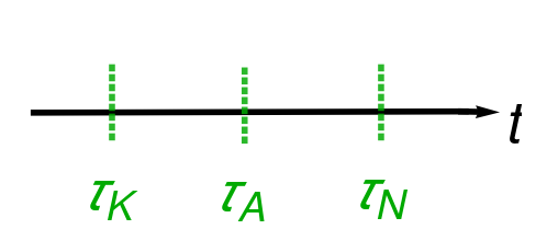
Figure 2: Illustration of three time scales in the model of harmonic chain of active particles - (i) Ο„K=1Ksubscript𝜏𝐾1𝐾\tau_{K}=\frac{1}{K} due to the interaction among particles, (ii) Ο„A=1Ξ³/1ΞΆ/1Dr​o​tsubscript𝜏𝐴1𝛾1𝜁1subscriptπ·π‘Ÿπ‘œπ‘‘\tau_{A}=\frac{1}{\gamma}~{}/\frac{1}{\zeta}~{}/\frac{1}{D_{rot}} due to the activity of AOUPΒ /Β RTPΒ /ABP and (iii) Ο„N=N2Ksubscriptπœπ‘superscript𝑁2𝐾\tau_{N}=\frac{N^{2}}{K} due to the finiteness of the ring. As shown in the figure, we will consider Ο„Kβ‰ͺΟ„Aβ‰ͺΟ„Nmuch-less-thansubscript𝜏𝐾subscript𝜏𝐴much-less-thansubscriptπœπ‘\tau_{K}\ll\tau_{A}\ll\tau_{N} in our paper.

Let us briefly summarize our findings. We study two point correlation

CΞ±1,Ξ±21​(t1,t2)=⟨xΞ±1​(t1)​xΞ±2​(t2)⟩c=⟨xΞ±1​(t1)​xΞ±2​(t2)βŸ©βˆ’βŸ¨xΞ±1​(t1)βŸ©β€‹βŸ¨xΞ±2​(t2)⟩,CΞ±1,Ξ±22​(t1,t2)=⟨yΞ±1​(t1)​yΞ±2​(t2)⟩c=⟨yΞ±1​(t1)​yΞ±2​(t2)βŸ©βˆ’βŸ¨yΞ±1​(t1)βŸ©β€‹βŸ¨yΞ±2​(t2)⟩.formulae-sequencesubscriptsuperscript𝐢1subscript𝛼1subscript𝛼2subscript𝑑1subscript𝑑2subscriptdelimited-⟨⟩subscriptπ‘₯subscript𝛼1subscript𝑑1subscriptπ‘₯subscript𝛼2subscript𝑑2𝑐delimited-⟨⟩subscriptπ‘₯subscript𝛼1subscript𝑑1subscriptπ‘₯subscript𝛼2subscript𝑑2delimited-⟨⟩subscriptπ‘₯subscript𝛼1subscript𝑑1delimited-⟨⟩subscriptπ‘₯subscript𝛼2subscript𝑑2subscriptsuperscript𝐢2subscript𝛼1subscript𝛼2subscript𝑑1subscript𝑑2subscriptdelimited-⟨⟩subscript𝑦subscript𝛼1subscript𝑑1subscript𝑦subscript𝛼2subscript𝑑2𝑐delimited-⟨⟩subscript𝑦subscript𝛼1subscript𝑑1subscript𝑦subscript𝛼2subscript𝑑2delimited-⟨⟩subscript𝑦subscript𝛼1subscript𝑑1delimited-⟨⟩subscript𝑦subscript𝛼2subscript𝑑2\displaystyle\begin{split}&C^{1}_{\alpha_{1},\alpha_{2}}(t_{1},t_{2})=\langle x_{\alpha_{1}}(t_{1})x_{\alpha_{2}}(t_{2})\rangle_{c}=\langle x_{\alpha_{1}}(t_{1})x_{\alpha_{2}}(t_{2})\rangle-\langle x_{\alpha_{1}}(t_{1})\rangle\langle x_{\alpha_{2}}(t_{2})\rangle,\\ &C^{2}_{\alpha_{1},\alpha_{2}}(t_{1},t_{2})=\langle y_{\alpha_{1}}(t_{1})y_{\alpha_{2}}(t_{2})\rangle_{c}=\langle y_{\alpha_{1}}(t_{1})y_{\alpha_{2}}(t_{2})\rangle-\langle y_{\alpha_{1}}(t_{1})\rangle\langle y_{\alpha_{2}}(t_{2})\rangle.\end{split} (11)

Once again, we emphasise that r→α​(t)=(xα​(t),0)subscriptβ†’π‘Ÿπ›Όπ‘‘subscriptπ‘₯𝛼𝑑0\vec{r}_{\alpha}(t)=(x_{\alpha}(t),0) for RTP and AOUP, and r→α​(t)=(xα​(t),yα​(t))subscriptβ†’π‘Ÿπ›Όπ‘‘subscriptπ‘₯𝛼𝑑subscript𝑦𝛼𝑑\vec{r}_{\alpha}(t)=\left(x_{\alpha}(t),y_{\alpha}(t)\right) for ABP. Consequently for RTP and AOUP, one has only the correlation CΞ±1,Ξ±21​(t1,t2)subscriptsuperscript𝐢1subscript𝛼1subscript𝛼2subscript𝑑1subscript𝑑2C^{1}_{\alpha_{1},\alpha_{2}}(t_{1},t_{2}), while for ABP one has both CΞ±1,Ξ±21/2​(t1,t2)subscriptsuperscript𝐢12subscript𝛼1subscript𝛼2subscript𝑑1subscript𝑑2C^{1/2}_{\alpha_{1},\alpha_{2}}(t_{1},t_{2}). Note that, since the noises ξα​(t)subscriptπœ‰π›Όπ‘‘\xi_{\alpha}(t) and ΟˆΞ²β€‹(t)subscriptπœ“π›½π‘‘\psi_{\beta}(t) are mutually uncorrelated [see Eq.Β (10)], the cross correlations among the xπ‘₯x and y𝑦y-coordinates for the particles in the ABP chain are zero i.e. ⟨xα​(t1)​yβ​(t2)⟩c=0subscriptdelimited-⟨⟩subscriptπ‘₯𝛼subscript𝑑1subscript𝑦𝛽subscript𝑑2𝑐0\langle x_{\alpha}(t_{1})y_{\beta}(t_{2})\rangle_{c}=0. We study CΞ±1,Ξ±21/2​(t1,t2)subscriptsuperscript𝐢12subscript𝛼1subscript𝛼2subscript𝑑1subscript𝑑2C^{1/2}_{\alpha_{1},\alpha_{2}}(t_{1},t_{2}) in different asymptotic regimes of time for three models of active particle chains of length N𝑁N. In all models the particles are connected to each other by harmonic springs of strength K𝐾K and each particle is driven by independent active noises Fβ†’A​(t)superscript→𝐹𝐴𝑑\vec{F}^{A}(t) which have different statistical properties. There are three time scales in this problem, namely, (i) the interaction time scale Ο„K=1Ksubscript𝜏𝐾1𝐾\tau_{K}=\frac{1}{K} (ii) the activity time scale Ο„Asubscript𝜏𝐴\tau_{A} and (iii) the relaxation time scale Ο„Nsubscriptπœπ‘\tau_{N}. The interaction time scale Ο„Ksubscript𝜏𝐾\tau_{K} is coming from interaction among the particles. The activity time scale Ο„Asubscript𝜏𝐴\tau_{A} arises due to the activity present in the system. The activity time scale Ο„A=1ΞΆsubscript𝜏𝐴1𝜁\tau_{A}=\frac{1}{\zeta} for RTP, Ο„A=1Ξ³subscript𝜏𝐴1𝛾\tau_{A}=\frac{1}{\gamma} for AOUP and Ο„A=1Dr​o​tsubscript𝜏𝐴1subscriptπ·π‘Ÿπ‘œπ‘‘\tau_{A}=\frac{1}{D_{rot}} for ABP particles. Finally, Ο„N=N2Ksubscriptπœπ‘superscript𝑁2𝐾\tau_{N}=\frac{N^{2}}{K} represents the relaxation time scale on a ring of size N𝑁N. Throughout this work, we will consider Ο„Kβ‰ͺΟ„Aβ‰ͺΟ„Nmuch-less-thansubscript𝜏𝐾subscript𝜏𝐴much-less-thansubscriptπœπ‘\tau_{K}\ll\tau_{A}\ll\tau_{N} (see Fig. 2). As illustrated in this work, with this order of time scales we find various interesting scaling structures and scaling functions for different position correlations. The other case of Ο„Aβ‰ͺΟ„Kβ‰ͺΟ„Nmuch-less-thansubscript𝜏𝐴subscript𝜏𝐾much-less-thansubscriptπœπ‘\tau_{A}\ll\tau_{K}\ll\tau_{N} does not give rise to these scaling structures and only reproduces the results of the passive particles.

More precisely, in this paper we study the two point correlation CΞ±1,Ξ±21/2​(t1,t2)subscriptsuperscript𝐢12subscript𝛼1subscript𝛼2subscript𝑑1subscript𝑑2C^{1/2}_{\alpha_{1},\alpha_{2}}(t_{1},t_{2}) in the following three regimes (i) t1,t2β‰ͺΟ„Kmuch-less-thansubscript𝑑1subscript𝑑2subscript𝜏𝐾t_{1},t_{2}\ll\tau_{K} (ii) Ο„Kβ‰ͺt1,t2β‰ͺΟ„Nformulae-sequencemuch-less-thansubscript𝜏𝐾subscript𝑑1much-less-thansubscript𝑑2subscriptπœπ‘\tau_{K}\ll t_{1},t_{2}\ll\tau_{N} with Nβ†’βˆžβ†’π‘N\to\infty (equivalently Ο„Nβ†’βˆžβ†’subscriptπœπ‘\tau_{N}\to\infty) (iii) t1,t2βˆΌΟ„Nsimilar-tosubscript𝑑1subscript𝑑2subscriptπœπ‘t_{1},t_{2}\sim\tau_{N} for finite but large N𝑁N. The MSD of a tagged particle, say α𝛼\alphath, is obtained from Οƒ1/22​(t)=CΞ±,Ξ±1/2​(t,t)subscriptsuperscript𝜎212𝑑subscriptsuperscript𝐢12𝛼𝛼𝑑𝑑\sigma^{2}_{1/2}(t)=C^{1/2}_{\alpha,\alpha}(t,t). Due to homogeneity and periodic boundary of the chain, the MSD of a tagged particle is independent of the tag of the particle. Covariance between the positions of two particles can similarly be obtained from C0,Ξ²1​(t)=⟨x0​(t)​xβ​(t)⟩csuperscriptsubscript𝐢0𝛽1𝑑subscriptdelimited-⟨⟩subscriptπ‘₯0𝑑subscriptπ‘₯𝛽𝑑𝑐C_{0,\beta}^{1}(t)=\langle x_{0}(t)x_{\beta}(t)\rangle_{c} and C0,Ξ²2​(t)=⟨y0​(t)​yβ​(t)⟩csuperscriptsubscript𝐢0𝛽2𝑑subscriptdelimited-⟨⟩subscript𝑦0𝑑subscript𝑦𝛽𝑑𝑐C_{0,\beta}^{2}(t)=\langle y_{0}(t)y_{\beta}(t)\rangle_{c} which are again same as ⟨xα​(t)​xΞ±+β​(t)⟩csubscriptdelimited-⟨⟩subscriptπ‘₯𝛼𝑑subscriptπ‘₯𝛼𝛽𝑑𝑐\langle x_{\alpha}(t)x_{\alpha+\beta}(t)\rangle_{c} and ⟨yα​(t)​yΞ±+β​(t)⟩csubscriptdelimited-⟨⟩subscript𝑦𝛼𝑑subscript𝑦𝛼𝛽𝑑𝑐\langle y_{\alpha}(t)y_{\alpha+\beta}(t)\rangle_{c} respectively due to translational symmetry of the problem. We also study position auto correlation CΞ±,Ξ±1/2​(t1,t2)superscriptsubscript𝐢𝛼𝛼12subscript𝑑1subscript𝑑2C_{\alpha,\alpha}^{1/2}(t_{1},t_{2}) and finally un-equal time correlation CΞ±1,Ξ±21/2​(t1,t2)superscriptsubscript𝐢subscript𝛼1subscript𝛼212subscript𝑑1subscript𝑑2C_{\alpha_{1},\alpha_{2}}^{1/2}(t_{1},t_{2}). We consider two cases: (a) Nβ†’βˆžβ†’π‘N\to\infty in which Ο„Nβ†’βˆžβ†’subscriptπœπ‘\tau_{N}\to\infty and (b) finite but large N𝑁N in which Ο„Nsubscriptπœπ‘\tau_{N} is finite. At times much smaller than Ο„Ksubscript𝜏𝐾\tau_{K}, the statistical properties of one particle are independent of other particles as in such short time they do not realise the presence of other particle. In this time regime, the correlation behaves as CΞ±1,Ξ±21/2​(t1,t2)∼CΞ±1,Ξ±11/2​(t1,t2)​δα1,Ξ±2similar-tosuperscriptsubscript𝐢subscript𝛼1subscript𝛼212subscript𝑑1subscript𝑑2superscriptsubscript𝐢subscript𝛼1subscript𝛼112subscript𝑑1subscript𝑑2subscript𝛿subscript𝛼1subscript𝛼2C_{\alpha_{1},\alpha_{2}}^{1/2}(t_{1},t_{2})\sim C_{\alpha_{1},\alpha_{1}}^{1/2}(t_{1},t_{2})\delta_{\alpha_{1},\alpha_{2}}. On the other hand, in case (a) we observe that the above four quantities exhibit interesting scaling behaviours for times much larger than Ο„Ksubscript𝜏𝐾\tau_{K}. For RTP and AOUP dynamics we get

CΞ±,Ξ±1​(t,t)superscriptsubscript𝐢𝛼𝛼1𝑑𝑑\displaystyle C_{\alpha,\alpha}^{1}(t,t) ∝t3/2​𝒯R​T/O​U​(tΟ„A),Ο„Kβ‰ͺtβ‰ͺΟ„Nformulae-sequenceproportional-toabsentsuperscript𝑑32superscriptπ’―π‘…π‘‡π‘‚π‘ˆπ‘‘subscript𝜏𝐴much-less-thansubscriptπœπΎπ‘‘much-less-thansubscriptπœπ‘\displaystyle\propto t^{3/2}~{}\mathcal{T}^{RT/OU}\left(\frac{t}{\tau_{A}}\right),~{}~{}~{}~{}~{}~{}~{}~{}~{}~{}~{}~{}\tau_{K}\ll t\ll\tau_{N} (12)
C0,Ξ²1​(t,t)superscriptsubscript𝐢0𝛽1𝑑𝑑\displaystyle C_{0,\beta}^{1}(t,t) ∝{tμ​ΩR​T/O​U​(Ξ²2​K​t);Ο„Kβ‰ͺtβ‰ͺΟ„Atβ€‹π’žβ€‹(Ξ²2​K​t);Ο„Aβ‰ͺtβ‰ͺΟ„N,proportional-toabsentcasessuperscriptπ‘‘πœ‡superscriptΞ©π‘…π‘‡π‘‚π‘ˆπ›½2𝐾𝑑much-less-thansubscriptπœπΎπ‘‘much-less-thansubscriptπœπ΄π‘‘π’žπ›½2𝐾𝑑much-less-thansubscriptπœπ΄π‘‘much-less-thansubscriptπœπ‘\displaystyle\propto\begin{cases}t^{\mu}~{}\Omega^{RT/OU}\left(\frac{\beta}{\sqrt{2Kt}}\right)~{};&~{}~{}~{}~{}~{}\tau_{K}\ll t\ll\tau_{A}\\ \sqrt{t}~{}\mathcal{C}\left(\frac{\beta}{\sqrt{2Kt}}\right)~{};&~{}~{}~{}~{}~{}\tau_{A}\ll t\ll\tau_{N},\end{cases} (13)
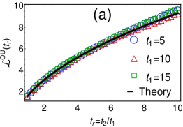
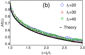
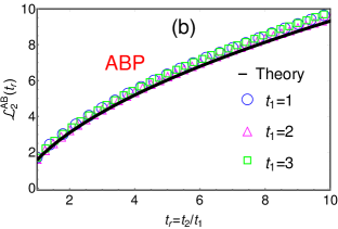
CΞ±,Ξ±1​(t1,t2)superscriptsubscript𝐢𝛼𝛼1subscript𝑑1subscript𝑑2\displaystyle C_{\alpha,\alpha}^{1}(t_{1},t_{2}) ∝{t1μ​ℒR​T/O​U​(t2t1);Ο„Kβ‰ͺt1β‰ͺΟ„At1​ℳ​(t2t1);Ο„Aβ‰ͺt1β‰ͺΟ„Nproportional-toabsentcasessuperscriptsubscript𝑑1πœ‡superscriptβ„’π‘…π‘‡π‘‚π‘ˆsubscript𝑑2subscript𝑑1much-less-thansubscript𝜏𝐾subscript𝑑1much-less-thansubscript𝜏𝐴subscript𝑑1β„³subscript𝑑2subscript𝑑1much-less-thansubscript𝜏𝐴subscript𝑑1much-less-thansubscriptπœπ‘\displaystyle\propto\begin{cases}t_{1}^{\mu}~{}\mathcal{L}^{RT/OU}\left(\frac{t_{2}}{t_{1}}\right)~{};&~{}~{}~{}~{}~{}~{}~{}~{}~{}\tau_{K}\ll t_{1}\ll\tau_{A}\\ \sqrt{t_{1}}~{}\mathcal{M}\left(\frac{t_{2}}{t_{1}}\right)~{};&~{}~{}~{}~{}~{}~{}~{}~{}~{}\tau_{A}\ll t_{1}\ll\tau_{N}\end{cases} (14)
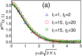
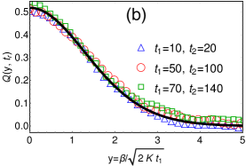
CΞ±1,Ξ±21​(t1,t2)superscriptsubscript𝐢subscript𝛼1subscript𝛼21subscript𝑑1subscript𝑑2\displaystyle C_{\alpha_{1},\alpha_{2}}^{1}(t_{1},t_{2}) ∝{t1μ​𝒫R​T/O​U​(Ξ²2​K​t1,t2t1);Ο„Kβ‰ͺt1β‰ͺΟ„At1​𝒬​(Ξ²2​K​t1,t2t1);Ο„Aβ‰ͺtβ‰ͺΟ„Nproportional-toabsentcasessuperscriptsubscript𝑑1πœ‡superscriptπ’«π‘…π‘‡π‘‚π‘ˆπ›½2𝐾subscript𝑑1subscript𝑑2subscript𝑑1much-less-thansubscript𝜏𝐾subscript𝑑1much-less-thansubscript𝜏𝐴subscript𝑑1𝒬𝛽2𝐾subscript𝑑1subscript𝑑2subscript𝑑1much-less-thansubscriptπœπ΄π‘‘much-less-thansubscriptπœπ‘\displaystyle\propto\begin{cases}t_{1}^{\mu}~{}\mathcal{P}^{RT/OU}\left(\frac{\beta}{\sqrt{2Kt_{1}}},\frac{t_{2}}{t_{1}}\right)~{};&\tau_{K}\ll t_{1}\ll\tau_{A}\\ \sqrt{t_{1}}~{}\mathcal{Q}\left(\frac{\beta}{\sqrt{2Kt_{1}}},\frac{t_{2}}{t_{1}}\right)~{};&\tau_{A}\ll t\ll\tau_{N}\end{cases} (15)

where ΞΌ=32πœ‡32\mu=\frac{3}{2} for RTP and ΞΌ=52πœ‡52\mu=\frac{5}{2} for AOUP. Also, the proportionality constants are given explicitly in the respective equations while deriving these results. Similarly for ABP, in case (a), we get

CΞ±,Ξ±p​(t,t)superscriptsubscript𝐢𝛼𝛼𝑝𝑑𝑑\displaystyle C_{\alpha,\alpha}^{p}(t,t) ∝t3/2​𝒯pA​B​(tΟ„A),Ο„Kβ‰ͺtβ‰ͺΟ„Nformulae-sequenceproportional-toabsentsuperscript𝑑32subscriptsuperscript𝒯𝐴𝐡𝑝𝑑subscript𝜏𝐴much-less-thansubscriptπœπΎπ‘‘much-less-thansubscriptπœπ‘\displaystyle\propto t^{3/2}~{}\mathcal{T}^{AB}_{p}\left(\frac{t}{\tau_{A}}\right),~{}~{}~{}~{}~{}~{}~{}~{}~{}~{}~{}~{}\tau_{K}\ll t\ll\tau_{N} (16)
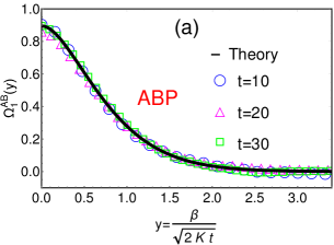
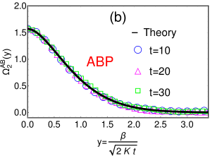
C0,Ξ²p​(t,t)superscriptsubscript𝐢0𝛽𝑝𝑑𝑑\displaystyle C_{0,\beta}^{p}(t,t) ∝{tν​ΩpA​B​(Ξ²2​K​t);Ο„Kβ‰ͺtβ‰ͺΟ„Atβ€‹π’žβ€‹(Ξ²2​K​t);Ο„Aβ‰ͺtβ‰ͺΟ„N,proportional-toabsentcasessuperscriptπ‘‘πœˆsubscriptsuperscriptΩ𝐴𝐡𝑝𝛽2𝐾𝑑much-less-thansubscriptπœπΎπ‘‘much-less-thansubscriptπœπ΄π‘‘π’žπ›½2𝐾𝑑much-less-thansubscriptπœπ΄π‘‘much-less-thansubscriptπœπ‘\displaystyle\propto\begin{cases}t^{\nu}~{}\Omega^{AB}_{p}\left(\frac{\beta}{\sqrt{2Kt}}\right)~{};&~{}~{}~{}~{}~{}\tau_{K}\ll t\ll\tau_{A}\\ \sqrt{t}~{}\mathcal{C}\left(\frac{\beta}{\sqrt{2Kt}}\right)~{};&~{}~{}~{}~{}~{}\tau_{A}\ll t\ll\tau_{N},\end{cases} (17)
CΞ±,Ξ±p​(t1,t2)superscriptsubscript𝐢𝛼𝛼𝑝subscript𝑑1subscript𝑑2\displaystyle C_{\alpha,\alpha}^{p}(t_{1},t_{2}) ∝{t1ν​ℒpA​B​(t2t1);Ο„Kβ‰ͺt1β‰ͺΟ„At1​ℳ​(t2t1);Ο„Aβ‰ͺt1β‰ͺΟ„Nproportional-toabsentcasessuperscriptsubscript𝑑1𝜈subscriptsuperscriptℒ𝐴𝐡𝑝subscript𝑑2subscript𝑑1much-less-thansubscript𝜏𝐾subscript𝑑1much-less-thansubscript𝜏𝐴subscript𝑑1β„³subscript𝑑2subscript𝑑1much-less-thansubscript𝜏𝐴subscript𝑑1much-less-thansubscriptπœπ‘\displaystyle\propto\begin{cases}t_{1}^{\nu}~{}\mathcal{L}^{AB}_{p}\left(\frac{t_{2}}{t_{1}}\right)~{};&~{}~{}~{}~{}~{}~{}~{}~{}~{}\tau_{K}\ll t_{1}\ll\tau_{A}\\ \sqrt{t_{1}}~{}\mathcal{M}\left(\frac{t_{2}}{t_{1}}\right)~{};&~{}~{}~{}~{}~{}~{}~{}~{}~{}\tau_{A}\ll t_{1}\ll\tau_{N}\end{cases} (18)
CΞ±1,Ξ±2p​(t1,t2)superscriptsubscript𝐢subscript𝛼1subscript𝛼2𝑝subscript𝑑1subscript𝑑2\displaystyle C_{\alpha_{1},\alpha_{2}}^{p}(t_{1},t_{2}) ∝{t1ν​𝒫pA​B​(Ξ²2​K​t1,t2t1);Ο„Kβ‰ͺt1β‰ͺΟ„At1​𝒬​(Ξ²2​K​t1,t2t1);Ο„Aβ‰ͺtβ‰ͺΟ„Nproportional-toabsentcasessuperscriptsubscript𝑑1𝜈subscriptsuperscript𝒫𝐴𝐡𝑝𝛽2𝐾subscript𝑑1subscript𝑑2subscript𝑑1much-less-thansubscript𝜏𝐾subscript𝑑1much-less-thansubscript𝜏𝐴subscript𝑑1𝒬𝛽2𝐾subscript𝑑1subscript𝑑2subscript𝑑1much-less-thansubscriptπœπ΄π‘‘much-less-thansubscriptπœπ‘\displaystyle\propto\begin{cases}t_{1}^{\nu}~{}\mathcal{P}^{AB}_{p}\left(\frac{\beta}{\sqrt{2Kt_{1}}},\frac{t_{2}}{t_{1}}\right)~{};&\tau_{K}\ll t_{1}\ll\tau_{A}\\ \sqrt{t_{1}}~{}\mathcal{Q}\left(\frac{\beta}{\sqrt{2Kt_{1}}},\frac{t_{2}}{t_{1}}\right)~{};&\tau_{A}\ll t\ll\tau_{N}\end{cases} (19)

where p=1​or​2𝑝1or2p=1~{}\text{or}~{}2 and Ξ½=72𝜈72\nu=\frac{7}{2} for p=1𝑝1p=1 and Ξ½=52𝜈52\nu=\frac{5}{2} for p=2𝑝2p=2.

For large but finite N𝑁N in case (b), we find that the correlation function C0,Ξ²p​(t1,t2)superscriptsubscript𝐢0𝛽𝑝subscript𝑑1subscript𝑑2C_{0,\beta}^{p}(t_{1},t_{2}) for all three models takes the scaling form

C0,Ξ²p​(t1,t2)≃2​De​f​f​NK​𝒲​(t2t1,Ξ²N,K​t1N2),t1,t2∼O​(Ο„N)formulae-sequencesimilar-to-or-equalssuperscriptsubscript𝐢0𝛽𝑝subscript𝑑1subscript𝑑22subscript𝐷𝑒𝑓𝑓𝑁𝐾𝒲subscript𝑑2subscript𝑑1𝛽𝑁𝐾subscript𝑑1superscript𝑁2subscript𝑑1similar-tosubscript𝑑2𝑂subscriptπœπ‘\displaystyle C_{0,\beta}^{p}(t_{1},t_{2})\simeq\frac{2D_{eff}N}{K}~{}\mathcal{W}\left(\frac{t_{2}}{t_{1}},\frac{\beta}{N},\frac{Kt_{1}}{N^{2}}\right),~{}~{}~{}t_{1},t_{2}\sim O(\tau_{N}) (20)

where De​f​fsubscript𝐷𝑒𝑓𝑓D_{eff} is the effective diffusion constants for the RTP (De​f​f=DR=v022​΢subscript𝐷𝑒𝑓𝑓subscript𝐷𝑅superscriptsubscript𝑣022𝜁D_{eff}=D_{R}=\frac{v_{0}^{2}}{2\zeta}), AOUP (De​f​f=DA=DΞ³2subscript𝐷𝑒𝑓𝑓subscript𝐷𝐴𝐷superscript𝛾2D_{eff}=D_{A}=\frac{D}{\gamma^{2}}) and ABP (De​f​f=DA​B​P=vA22​Dr​o​tsubscript𝐷𝑒𝑓𝑓subscript𝐷𝐴𝐡𝑃superscriptsubscript𝑣𝐴22subscriptπ·π‘Ÿπ‘œπ‘‘D_{eff}=D_{ABP}=\frac{v_{A}^{2}}{2D_{rot}}) chains. A summary of these results are given in Tables 1 and 2.

In what follows, we will study various statistical properties of the position of the tagged particles. We will first consider the mean squared displacement and covariance as functions of time which are followed by the studies of un-equal time two-point position correlations. We first compute these quantities for RTP and then for AOUP and ABP in the subsequent sections.
Refer to caption
Refer to caption
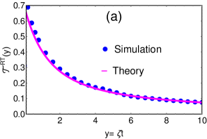
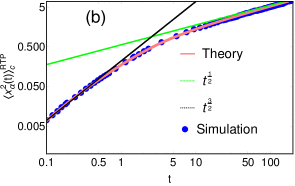
Figure 3: In Figure (a), we have plotted the scaling function 𝒯R​T​(y)superscript𝒯𝑅𝑇𝑦\mathcal{T}^{RT}(y) in Eq. (37) for RTP and compared with the results of numerical simulation. The Figure (b) shows the asymptotic forms of ⟨xΞ±2​(t)⟩cR​T​Psuperscriptsubscriptdelimited-⟨⟩superscriptsubscriptπ‘₯𝛼2𝑑𝑐𝑅𝑇𝑃\langle x_{\alpha}^{2}(t)\rangle_{c}^{RTP} derived in Eqs. (41) for Ο„Kβ‰ͺtβ‰ͺΟ„Amuch-less-thansubscriptπœπΎπ‘‘much-less-thansubscript𝜏𝐴\tau_{K}\ll t\ll\tau_{A} (shown by black dotted line) and Ο„Kβ‰ͺΟ„Aβ‰ͺtmuch-less-thansubscript𝜏𝐾subscript𝜏𝐴much-less-than𝑑\tau_{K}\ll\tau_{A}\ll t (shown by green dotted line) where Ο„A=1ΞΆsubscript𝜏𝐴1𝜁\tau_{A}=\frac{1}{\zeta}. The solid pink line corresponds to the theoretical result of ⟨xΞ±2​(t)⟩csubscriptdelimited-⟨⟩superscriptsubscriptπ‘₯𝛼2𝑑𝑐\langle x_{\alpha}^{2}(t)\rangle_{c} obtained in Eq. (36). For both plots, we have chosen K=2,ΞΆ=0.5formulae-sequence𝐾2𝜁0.5K=2,~{}\zeta=0.5 and v0=1subscript𝑣01v_{0}=1. The simulation is done with N=100𝑁100N=100 particles on a ring.

3 TWO POINT CORRELATION FOR RTP CHAIN

We begin by computing the two point correlation function CΞ±,Ξ²1​(t1,t2)superscriptsubscript𝐢𝛼𝛽1subscript𝑑1subscript𝑑2C_{\alpha,\beta}^{1}(t_{1},t_{2}) in Eq. (11) when the particles perform RTP dynamics. Recall that the RTP dynamics is considered in one dimension and r→α​(t)=(xα​(t),0)subscriptβ†’π‘Ÿπ›Όπ‘‘subscriptπ‘₯𝛼𝑑0\vec{r}_{\alpha}(t)=(x_{\alpha}(t),0) in Eq. (11). Let us first look at the case when t1=t2=tsubscript𝑑1subscript𝑑2𝑑t_{1}=t_{2}=t in CΞ±,Ξ²1​(t1,t2)superscriptsubscript𝐢𝛼𝛽1subscript𝑑1subscript𝑑2C_{\alpha,\beta}^{1}(t_{1},t_{2}). To proceed, we perform Fourier transform with respect to α𝛼\alpha on both sides of the set of Langevin Eqs. (1). For a general function gα​(t)subscript𝑔𝛼𝑑g_{\alpha}(t), we define the Fourier transformation as

gα​(t)=βˆ‘s=0Nβˆ’1e2​π​i​sN​α​gΒ―s​(t),subscript𝑔𝛼𝑑superscriptsubscript𝑠0𝑁1superscript𝑒2πœ‹π‘–π‘ π‘π›Όsubscript¯𝑔𝑠𝑑\displaystyle g_{\alpha}(t)=\sum_{s=0}^{N-1}e^{\frac{2\pi is}{N}\alpha}~{}\bar{g}_{s}(t), (21)

where i2=βˆ’1superscript𝑖21i^{2}=-1 and the inverse Fourier transformation as

gΒ―s​(t)=1Nβ€‹βˆ‘Ξ±=0Nβˆ’1eβˆ’2​π​i​sN​α​gα​(t).subscript¯𝑔𝑠𝑑1𝑁superscriptsubscript𝛼0𝑁1superscript𝑒2πœ‹π‘–π‘ π‘π›Όsubscript𝑔𝛼𝑑\displaystyle\bar{g}_{s}(t)=\frac{1}{N}\sum_{\alpha=0}^{N-1}e^{-\frac{2\pi is}{N}\alpha}~{}g_{\alpha}(t). (22)

Writing the Langevin Eqs. (1) in terms of the Fourier variables

d​xΒ―sd​t=βˆ’as​xΒ―s+FΒ―sA​(t),𝑑subscriptΒ―π‘₯𝑠𝑑𝑑subscriptπ‘Žπ‘ subscriptΒ―π‘₯𝑠superscriptsubscript¯𝐹𝑠𝐴𝑑\displaystyle\frac{d\bar{x}_{s}}{dt}=-a_{s}\bar{x}_{s}+\bar{F}_{s}^{A}(t)~{}, (23)

one now gets rid of the cross terms. Also here

xΒ―s​(t)=1Nβ€‹βˆ‘Ξ±=0Nβˆ’1eβˆ’2​π​i​sN​α​xα​(t),subscriptΒ―π‘₯𝑠𝑑1𝑁superscriptsubscript𝛼0𝑁1superscript𝑒2πœ‹π‘–π‘ π‘π›Όsubscriptπ‘₯𝛼𝑑\displaystyle\bar{x}_{s}(t)=\frac{1}{N}\sum_{\alpha=0}^{N-1}e^{-\frac{2\pi is}{N}\alpha}~{}x_{\alpha}(t), (24)
FΒ―sA​(t)=1Nβ€‹βˆ‘Ξ±=0Nβˆ’1eβˆ’2​π​i​sN​α​FΞ±A​(t),subscriptsuperscript¯𝐹𝐴𝑠𝑑1𝑁superscriptsubscript𝛼0𝑁1superscript𝑒2πœ‹π‘–π‘ π‘π›Όsuperscriptsubscript𝐹𝛼𝐴𝑑\displaystyle\bar{F}^{A}_{s}(t)=\frac{1}{N}\sum_{\alpha=0}^{N-1}e^{-\frac{2\pi is}{N}\alpha}~{}F_{\alpha}^{A}(t), (25)
as=4​K​sin2⁑(π​sN).subscriptπ‘Žπ‘ 4𝐾superscript2πœ‹π‘ π‘\displaystyle a_{s}=4K\sin^{2}\left(\frac{\pi s}{N}\right). (26)

It is now straightforward to solve Eq. (23) for xΒ―s​(t)subscriptΒ―π‘₯𝑠𝑑\bar{x}_{s}(t) to get

xΒ―s​(t)=eβˆ’as​t​xΒ―s​(0)+eβˆ’as​tβ€‹βˆ«0t𝑑τ​eas​τ​FΒ―sA​(Ο„),subscriptΒ―π‘₯𝑠𝑑superscript𝑒subscriptπ‘Žπ‘ π‘‘subscriptΒ―π‘₯𝑠0superscript𝑒subscriptπ‘Žπ‘ π‘‘superscriptsubscript0𝑑differential-d𝜏superscript𝑒subscriptπ‘Žπ‘ πœsuperscriptsubscriptΒ―πΉπ‘ π΄πœ\displaystyle\bar{x}_{s}(t)=e^{-a_{s}t}~{}\bar{x}_{s}(0)+e^{-a_{s}t}\int_{0}^{t}d\tau~{}e^{a_{s}\tau}~{}\bar{F}_{s}^{A}(\tau), (27)

using which in Eq.Β (21) we get the displacement xα​(t)subscriptπ‘₯𝛼𝑑x_{\alpha}(t) of the Ξ±thsuperscript𝛼th\alpha^{\text{th}} particle.

Remember we are interested to compute the two point correlation defined in Eq.Β (11) which after some manipulations can be written as

⟨xΞ±1​(t1)​xΞ±2​(t2)⟩c=βˆ‘s=0Nβˆ’1βˆ‘s=0Nβˆ’1e2​π​i​sN​α1​e2​π​i​sβ€²N​α2β€‹βŸ¨xΒ―s​(t)​xΒ―sβ€²βˆ—β€‹(t)⟩csubscriptdelimited-⟨⟩subscriptπ‘₯subscript𝛼1subscript𝑑1subscriptπ‘₯subscript𝛼2subscript𝑑2𝑐superscriptsubscript𝑠0𝑁1superscriptsubscript𝑠0𝑁1superscript𝑒2πœ‹π‘–π‘ π‘subscript𝛼1superscript𝑒2πœ‹π‘–superscript𝑠′𝑁subscript𝛼2subscriptdelimited-⟨⟩subscriptΒ―π‘₯𝑠𝑑superscriptsubscriptΒ―π‘₯superscript𝑠′𝑑𝑐\displaystyle\langle x_{\alpha_{1}}(t_{1})x_{\alpha_{2}}(t_{2})\rangle_{c}=\sum_{s=0}^{N-1}\sum_{s=0}^{N-1}e^{\frac{2\pi is}{N}\alpha_{1}}e^{\frac{2\pi is^{\prime}}{N}\alpha_{2}}\langle\bar{x}_{s}(t)\bar{x}_{s^{\prime}}^{*}(t)\rangle_{c} (28)

where

⟨xΒ―s​(t)​xΒ―sβ€²βˆ—β€‹(t)⟩c=⟨xΒ―s​(t)​xΒ―sβ€²βˆ—β€‹(t)βŸ©βˆ’βŸ¨xΒ―s​(t)βŸ©β€‹βŸ¨xΒ―sβ€²βˆ—β€‹(t)⟩=eβˆ’(as+asβ€²)​tβ€‹βˆ«0t𝑑τ1​𝑑τ2​eas​τ1+as′​τ2β€‹βŸ¨FΒ―sA​(Ο„1)​FΒ―sβ€²Aβ£βˆ—β€‹(Ο„2)⟩c,subscriptdelimited-⟨⟩subscriptΒ―π‘₯𝑠𝑑superscriptsubscriptΒ―π‘₯superscript𝑠′𝑑𝑐delimited-⟨⟩subscriptΒ―π‘₯𝑠𝑑superscriptsubscriptΒ―π‘₯superscript𝑠′𝑑delimited-⟨⟩subscriptΒ―π‘₯𝑠𝑑delimited-⟨⟩superscriptsubscriptΒ―π‘₯superscript𝑠′𝑑superscript𝑒subscriptπ‘Žπ‘ subscriptπ‘Žsuperscript𝑠′𝑑superscriptsubscript0𝑑differential-dsubscript𝜏1differential-dsubscript𝜏2superscript𝑒subscriptπ‘Žπ‘ subscript𝜏1subscriptπ‘Žsuperscript𝑠′subscript𝜏2subscriptdelimited-⟨⟩superscriptsubscript¯𝐹𝑠𝐴subscript𝜏1superscriptsubscript¯𝐹superscript𝑠′𝐴subscript𝜏2𝑐\displaystyle\begin{split}\langle\bar{x}_{s}(t)\bar{x}_{s^{\prime}}^{*}(t)\rangle_{c}&={\langle\bar{x}_{s}(t)\bar{x}_{s^{\prime}}^{*}(t)\rangle-\langle\bar{x}_{s}(t)\rangle\langle\bar{x}_{s^{\prime}}^{*}(t)\rangle}\\ &=e^{-(a_{s}+a_{s^{\prime}})t}\int_{0}^{t}d\tau_{1}~{}d\tau_{2}~{}e^{a_{s}\tau_{1}+a_{s^{\prime}}\tau_{2}}~{}\langle\bar{F}_{s}^{A}(\tau_{1})\bar{F}_{s^{\prime}}^{A*}(\tau_{2})\rangle_{c},\end{split} (29)

where xΒ―sβˆ—β€‹(t)superscriptsubscriptΒ―π‘₯𝑠𝑑\bar{x}_{s}^{*}(t) is the complex conjugate of xΒ―s​(t)subscriptΒ―π‘₯𝑠𝑑\bar{x}_{s}(t) and βŸ¨β€¦βŸ©delimited-βŸ¨βŸ©β€¦\langle...\rangle denotes average over noise σ¯s​(t)subscriptΒ―πœŽπ‘ π‘‘\bar{\sigma}_{s}(t) for RTP. We substitute FΞ±A​(t)subscriptsuperscript𝐹𝐴𝛼𝑑F^{A}_{\alpha}(t) from Eq. (3) for RTP in Eq. (25) to get FΒ―sA​(t)subscriptsuperscript¯𝐹𝐴𝑠𝑑\bar{F}^{A}_{s}(t). Inserting this expression in Eq. (29) and performing the integration over Ο„1subscript𝜏1\tau_{1} and Ο„2subscript𝜏2\tau_{2} gives ⟨xΒ―s​(t)​xΒ―sβ€²βˆ—β€‹(t)⟩csubscriptdelimited-⟨⟩subscriptΒ―π‘₯𝑠𝑑superscriptsubscriptΒ―π‘₯superscript𝑠′𝑑𝑐\langle\bar{x}_{s}(t)\bar{x}_{s^{\prime}}^{*}(t)\rangle_{c}. For continuity of the presentation, we have relegated the details of this calculation to A and present only the final results here. The final expressions for the correlations read

⟨xΒ―s​(t)​xΒ―sβ€²βˆ—β€‹(t)⟩cR​T​Psuperscriptsubscriptdelimited-⟨⟩subscriptΒ―π‘₯𝑠𝑑superscriptsubscriptΒ―π‘₯superscript𝑠′𝑑𝑐𝑅𝑇𝑃\displaystyle\langle\bar{x}_{s}(t)\bar{x}_{s^{\prime}}^{*}(t)\rangle_{c}^{RTP} =Ξ΄s,s′​v02N​𝒒​(2​΢,as,t),absentsubscript𝛿𝑠superscript𝑠′superscriptsubscript𝑣02𝑁𝒒2𝜁subscriptπ‘Žπ‘ π‘‘\displaystyle=\delta_{s,s^{\prime}}\frac{v_{0}^{2}}{N}~{}\mathcal{G}(2\zeta,a_{s},t), (30)

where Ξ΄s,sβ€²subscript𝛿𝑠superscript𝑠′\delta_{s,s^{\prime}} is the Kronecker delta which takes value 111 if s=s′𝑠superscript𝑠′s=s^{\prime} and 00 otherwise. Also here, 𝒒​(a,b,t)π’’π‘Žπ‘π‘‘\mathcal{G}(a,b,t) is defined as

𝒒​(a,b,t)π’’π‘Žπ‘π‘‘\displaystyle\mathcal{G}(a,b,t) =b​[1+eβˆ’2​b​tβˆ’2​eβˆ’(a+b)​t]βˆ’a​(1βˆ’eβˆ’2​b​t)b​(b2βˆ’a2).absent𝑏delimited-[]1superscript𝑒2𝑏𝑑2superscriptπ‘’π‘Žπ‘π‘‘π‘Ž1superscript𝑒2𝑏𝑑𝑏superscript𝑏2superscriptπ‘Ž2\displaystyle=\frac{b\left[1+e^{-2bt}-2e^{-(a+b)t}\right]-a(1-e^{-2bt})}{b(b^{2}-a^{2})}. (31)

3.1 MSD for RTP chain

To compute the MSD, we use Eq. (24) to write xα​(t)subscriptπ‘₯𝛼𝑑x_{\alpha}(t) in terms of xΒ―s​(t)subscriptΒ―π‘₯𝑠𝑑\bar{x}_{s}(t) and then substitute the correlation in Eq. (30) to get

⟨xΞ±2​(t)⟩cR​T​Psuperscriptsubscriptdelimited-⟨⟩superscriptsubscriptπ‘₯𝛼2𝑑𝑐𝑅𝑇𝑃\displaystyle\langle x_{\alpha}^{2}(t)\rangle_{c}^{RTP} =⟨xΞ±2​(t)⟩R​T​Pβˆ’(⟨xα​(t)⟩R​T​P)2absentsuperscriptdelimited-⟨⟩superscriptsubscriptπ‘₯𝛼2𝑑𝑅𝑇𝑃superscriptsuperscriptdelimited-⟨⟩subscriptπ‘₯𝛼𝑑𝑅𝑇𝑃2\displaystyle=\langle x_{\alpha}^{2}(t)\rangle^{RTP}-\left(\langle x_{\alpha}(t)\rangle^{RTP}\right)^{2}
=βˆ‘s=0Nβˆ’1⟨|xΒ―s​(t)|2⟩cR​T​P,absentsuperscriptsubscript𝑠0𝑁1superscriptsubscriptdelimited-⟨⟩superscriptsubscriptΒ―π‘₯𝑠𝑑2𝑐𝑅𝑇𝑃\displaystyle=\sum_{s=0}^{N-1}\langle|\bar{x}_{s}(t)|^{2}\rangle_{c}^{RTP},
=v02Nβ€‹βˆ‘s=0Nβˆ’1𝒒​(2​΢,as,t),absentsuperscriptsubscript𝑣02𝑁superscriptsubscript𝑠0𝑁1𝒒2𝜁subscriptπ‘Žπ‘ π‘‘\displaystyle=\frac{v_{0}^{2}}{N}\sum_{s=0}^{N-1}\mathcal{G}(2\zeta,a_{s},t), (32)

with assubscriptπ‘Žπ‘ a_{s} and 𝒒​(2​΢,as,t)𝒒2𝜁subscriptπ‘Žπ‘ π‘‘\mathcal{G}(2\zeta,a_{s},t) given respectively in Eqs. (26) and (31). Note that, due to the translational symmetry in α𝛼\alpha, the R.H.S. of ⟨xΞ±2​(t)⟩cR​T​Psuperscriptsubscriptdelimited-⟨⟩superscriptsubscriptπ‘₯𝛼2𝑑𝑐𝑅𝑇𝑃\langle x_{\alpha}^{2}(t)\rangle_{c}^{RTP} is independent of α𝛼\alpha. To gain more understanding of ⟨xΞ±2​(t)⟩cR​T​Psuperscriptsubscriptdelimited-⟨⟩superscriptsubscriptπ‘₯𝛼2𝑑𝑐𝑅𝑇𝑃\langle x_{\alpha}^{2}(t)\rangle_{c}^{RTP}, we first analyze the expression in the limit Nβ†’βˆžβ†’π‘N\to\infty. In this limit, the summation in the R.H.S. of Eq. (32) can be changed to an integral as 1Nβ€‹βˆ‘sβ†’12β€‹Ο€β€‹βˆ«βˆ’Ο€Ο€π‘‘qβ†’1𝑁subscript𝑠12πœ‹superscriptsubscriptπœ‹πœ‹differential-dπ‘ž\frac{1}{N}\sum_{s}\to\frac{1}{2\pi}\int_{-\pi}^{\pi}dq where q=2​π​sNπ‘ž2πœ‹π‘ π‘q=\frac{2\pi s}{N}. Changing the summation to integration in Eq. (32), we get

⟨xΞ±2​(t)⟩cR​T​Psuperscriptsubscriptdelimited-⟨⟩superscriptsubscriptπ‘₯𝛼2𝑑𝑐𝑅𝑇𝑃\displaystyle\langle x_{\alpha}^{2}(t)\rangle_{c}^{RTP} ≃v022β€‹Ο€β€‹βˆ«βˆ’Ο€Ο€π‘‘q​𝒒​(2​΢,bq,t),similar-to-or-equalsabsentsuperscriptsubscript𝑣022πœ‹superscriptsubscriptπœ‹πœ‹differential-dπ‘žπ’’2𝜁subscriptπ‘π‘žπ‘‘\displaystyle\simeq\frac{v_{0}^{2}}{2\pi}\int_{-\pi}^{\pi}dq~{}\mathcal{G}\left(2\zeta,b_{q},t\right), (33)
where​bqwheresubscriptπ‘π‘ž\displaystyle\text{where}~{}~{}b_{q} =4​K​sin2⁑(q/2).absent4𝐾superscript2π‘ž2\displaystyle=4K\sin^{2}(q/2). (34)

As mentioned before (see discussion below Eq. (11)), we are interested in Ο„Kβ‰ͺΟ„Amuch-less-thansubscript𝜏𝐾subscript𝜏𝐴\tau_{K}\ll\tau_{A} in this work with Ο„Nβ†’βˆžβ†’subscriptπœπ‘\tau_{N}\to\infty as Nβ†’βˆžβ†’π‘N\to\infty. Remember in this case Ο„A=1ΞΆsubscript𝜏𝐴1𝜁\tau_{A}=\frac{1}{\zeta}. We first look at the mean squared displacement for tβ‰ͺΟ„Kmuch-less-than𝑑subscript𝜏𝐾t\ll\tau_{K} followed by a discussion for t≫τKmuch-greater-than𝑑subscript𝜏𝐾t\gg\tau_{K}.

Since Ο„Ksubscript𝜏𝐾\tau_{K} is the smallest time scale in the model, the observation time t𝑑t is smaller than all the time scales (see Fig. 2). We can, then, consider ⟨xΞ±2​(t)⟩csubscriptdelimited-⟨⟩superscriptsubscriptπ‘₯𝛼2𝑑𝑐\langle x_{\alpha}^{2}(t)\rangle_{c} in Eq. (33) upto leading order in t𝑑t. Expanding 𝒒​(2​΢,bq,t)𝒒2𝜁subscriptπ‘π‘žπ‘‘\mathcal{G}(2\zeta,b_{q},t) in Eq. (31) in small t𝑑t, we find that 𝒒​(2​΢,bq,t)≃t2similar-to-or-equals𝒒2𝜁subscriptπ‘π‘žπ‘‘superscript𝑑2\mathcal{G}(2\zeta,b_{q},t)\simeq t^{2}. Inserting this in the expression of ⟨xΞ±2​(t)⟩csubscriptdelimited-⟨⟩superscriptsubscriptπ‘₯𝛼2𝑑𝑐\langle x_{\alpha}^{2}(t)\rangle_{c} and performing the integration over qπ‘žq gives

⟨xΞ±2​(t)⟩cR​T​P≃v02​t2,for ​tβ‰ͺΟ„K.formulae-sequencesimilar-to-or-equalssuperscriptsubscriptdelimited-⟨⟩superscriptsubscriptπ‘₯𝛼2𝑑𝑐𝑅𝑇𝑃superscriptsubscript𝑣02superscript𝑑2much-less-thanfor 𝑑subscript𝜏𝐾\displaystyle\langle x_{\alpha}^{2}(t)\rangle_{c}^{RTP}\simeq v_{0}^{2}t^{2},~{}~{}~{}~{}~{}~{}~{}\text{for }t\ll\tau_{K}. (35)

For small t𝑑t, the particles do not feel the presence of the neighbouring particles and move ballistically with speed v0subscript𝑣0v_{0}. This observation essentially asserts the form of ⟨xΞ±2​(t)⟩cR​T​Psuperscriptsubscriptdelimited-⟨⟩superscriptsubscriptπ‘₯𝛼2𝑑𝑐𝑅𝑇𝑃\langle x_{\alpha}^{2}(t)\rangle_{c}^{RTP} in Eq. (35).

We now look at the other limit when t≫τKmuch-greater-than𝑑subscript𝜏𝐾t\gg\tau_{K}. Substituing the expression of 𝒒​(2​΢,bq,t)𝒒2𝜁subscriptπ‘π‘žπ‘‘\mathcal{G}\left(2\zeta,b_{q},t\right) and bqsubscriptπ‘π‘žb_{q} from Eqs. (31) and (34) respectively in ⟨xΞ±2​(t)⟩cR​T​Psuperscriptsubscriptdelimited-⟨⟩superscriptsubscriptπ‘₯𝛼2𝑑𝑐𝑅𝑇𝑃\langle x_{\alpha}^{2}(t)\rangle_{c}^{RTP} in Eq. (33), we find integrals of the form βˆΌβˆ«π‘‘q​h​(q)​exp​[βˆ’K​t​sin2⁑(q/2)]similar-toabsentdifferential-dπ‘žβ„Žπ‘žexpdelimited-[]𝐾𝑑superscript2π‘ž2\sim\int dq~{}h(q)~{}\text{exp}\left[-Kt\sin^{2}(q/2)\right] where h​(q)β„Žπ‘žh(q) is some function of qπ‘žq. For K​tβ†’βˆžβ†’πΎπ‘‘Kt\to\infty, such integrals will be dominated by the small values of qπ‘žq. Therefore, we approximate bq≃K​q2similar-to-or-equalssubscriptπ‘π‘žπΎsuperscriptπ‘ž2b_{q}\simeq Kq^{2} in Eq. (33). We have explicitly computed ⟨xΞ±2​(t)⟩cR​T​Psuperscriptsubscriptdelimited-⟨⟩superscriptsubscriptπ‘₯𝛼2𝑑𝑐𝑅𝑇𝑃\langle x_{\alpha}^{2}(t)\rangle_{c}^{RTP} for t≫τKmuch-greater-than𝑑subscript𝜏𝐾t\gg\tau_{K} in B. The final approximate expression obeys the scaling form

⟨xΞ±2​(t)⟩cR​T​P≃v02​t32π​2K​𝒯R​T​(΢​t),similar-to-or-equalssuperscriptsubscriptdelimited-⟨⟩superscriptsubscriptπ‘₯𝛼2𝑑𝑐𝑅𝑇𝑃superscriptsubscript𝑣02superscript𝑑32πœ‹2𝐾superscriptπ’―π‘…π‘‡πœπ‘‘\displaystyle\langle x_{\alpha}^{2}(t)\rangle_{c}^{RTP}\simeq\frac{v_{0}^{2}t^{\frac{3}{2}}}{\pi}\sqrt{\frac{2}{K}}~{}~{}\mathcal{T}^{RT}\left(\zeta t\right), (36)

where the scaling function 𝒯R​T​(y)superscript𝒯𝑅𝑇𝑦\mathcal{T}^{RT}(y) is given by,

𝒯R​T​(y)=14β€‹βˆ«βˆ’βˆžβˆžπ‘‘w​𝒒​(2​y,w22,1),for ​t≫τKformulae-sequencesuperscript𝒯𝑅𝑇𝑦14superscriptsubscriptdifferential-d𝑀𝒒2𝑦superscript𝑀221much-greater-thanfor 𝑑subscript𝜏𝐾\displaystyle\mathcal{T}^{RT}(y)=\frac{1}{4}\int_{-\infty}^{\infty}dw~{}\mathcal{G}\left(2y,\frac{w^{2}}{2},1\right),~{}~{}~{}~{}~{}~{}~{}~{}\text{for }t\gg\tau_{K} (37)

with 𝒒​(2​y,w22,1)𝒒2𝑦superscript𝑀221\mathcal{G}\left(2y,\frac{w^{2}}{2},1\right) given in Eq. (31). In Fig.Β 3(a), we have plotted the scaling function 𝒯R​T​(y)superscript𝒯𝑅𝑇𝑦\mathcal{T}^{RT}(y) and compared it with the numerical simulation. We observe an excellent match between them. Expanding 𝒒​(2​y,w22,1)𝒒2𝑦superscript𝑀221\mathcal{G}\left(2y,\frac{w^{2}}{2},1\right) in various limits of y𝑦y, it is easy to see that 𝒯R​T​(y)superscript𝒯𝑅𝑇𝑦\mathcal{T}^{RT}(y) has the following asymptotic forms

𝒯R​T​(y)superscript𝒯𝑅𝑇𝑦\displaystyle\mathcal{T}^{RT}(y) ≃2​π3​(2βˆ’2)βˆ’4​π15​(8βˆ’5​2)​y,as ​yβ†’0,formulae-sequencesimilar-to-or-equalsabsent2πœ‹3224πœ‹15852𝑦→as 𝑦0\displaystyle\simeq\frac{2\sqrt{\pi}}{3}(2-\sqrt{2})-{\frac{4\sqrt{\pi}}{15}\left(8-5\sqrt{2}\right)y},~{}~{}~{}~{}\text{as }y\to 0, (38)
≃π2​y+O​(1y2),as ​yβ†’βˆž.formulae-sequencesimilar-to-or-equalsabsentπœ‹2𝑦𝑂1superscript𝑦2β†’as 𝑦\displaystyle\simeq\frac{\sqrt{\pi}}{2y}+{O\left(\frac{1}{y^{2}}\right)},~{}~{}~{}~{}~{}~{}~{}~{}~{}~{}~{}~{}~{}~{}~{}~{}~{}~{}~{}~{}~{}~{}~{}~{}~{}~{}~{}~{}~{}~{}\text{as }y\to\infty. (39)

Using these asymptotic forms in the expression of ⟨xΞ±2​(t)⟩cR​T​Psuperscriptsubscriptdelimited-⟨⟩superscriptsubscriptπ‘₯𝛼2𝑑𝑐𝑅𝑇𝑃\langle x_{\alpha}^{2}(t)\rangle_{c}^{RTP} in Eq. (36), we observe that it crosses from t3/2superscript𝑑32t^{3/2} for tβ‰ͺ1ΞΆmuch-less-than𝑑1𝜁t\ll\frac{1}{\zeta} to t𝑑\sqrt{t} for t≫1ΞΆmuch-greater-than𝑑1𝜁t\gg\frac{1}{\zeta}

⟨xΞ±2​(t)⟩cR​T​Psuperscriptsubscriptdelimited-⟨⟩superscriptsubscriptπ‘₯𝛼2𝑑𝑐𝑅𝑇𝑃\displaystyle\langle x_{\alpha}^{2}(t)\rangle_{c}^{RTP} ≃4​(2βˆ’1)3​π​K​v02​t32+O​(t5/2),for ​tβ‰ͺ1ΞΆ,formulae-sequencesimilar-to-or-equalsabsent4213πœ‹πΎsuperscriptsubscript𝑣02superscript𝑑32𝑂superscript𝑑52much-less-thanfor 𝑑1𝜁\displaystyle\simeq\frac{4(\sqrt{2}-1)}{3\sqrt{\pi K}}v_{0}^{2}t^{\frac{3}{2}}+{O\left(t^{5/2}\right)},~{}~{}~{}~{}~{}~{}~{}~{}\text{for }t\ll\frac{1}{\zeta}, (40)
≃v022​΢​2​tπ​K+O​(tβˆ’1/2),for ​t≫1ΞΆ.formulae-sequencesimilar-to-or-equalsabsentsuperscriptsubscript𝑣022𝜁2π‘‘πœ‹πΎπ‘‚superscript𝑑12much-greater-thanfor 𝑑1𝜁\displaystyle\simeq\frac{v_{0}^{2}}{2\zeta}\sqrt{\frac{2t}{\pi K}}+{O\left(t^{-1/2}\right)},~{}~{}~{}~{}~{}~{}~{}~{}~{}~{}~{}~{}~{}~{}\text{for }t\gg\frac{1}{\zeta}. (41)

For t≫1ΞΆmuch-greater-than𝑑1𝜁t\gg\frac{1}{\zeta}, the RTPs behave like Brownian particles with an effective diffusion constant DR=v022​΢subscript𝐷𝑅superscriptsubscript𝑣022𝜁D_{R}=\frac{v_{0}^{2}}{2\zeta}. For Nβ†’βˆžβ†’π‘N\to\infty, the motion of the tagged particle is effectively like single file diffusion which gives rise to the ∼tsimilar-toabsent𝑑\sim\sqrt{t} scaling for the MSD. This behaviour of the MSD for persistent random walkers in one dimensional lattice with hardcore interactions was obtained in [72, 75]. On the other hand, for Ο„Kβ‰ͺtβ‰ͺ1ΞΆmuch-less-thansubscriptπœπΎπ‘‘much-less-than1𝜁\tau_{K}\ll t\ll\frac{1}{\zeta}, we obtain that the MSD for RTPs scales super-diffusively as ∼t3/2similar-toabsentsuperscript𝑑32\sim t^{3/2} in contrast to the t2superscript𝑑2t^{2} scaling for non-interacting RTPs. We emphasise that the t3/2superscript𝑑32t^{3/2} scaling of the MSD arises due to the interplay of the activity of the particles and interactions between them. Due to the interaction with other particles, the motion of the tagged particle is hemmed and we consequently get t3/2superscript𝑑32t^{3/2} scaling for the MSD. The t3/2superscript𝑑32t^{3/2} behaviour for the MSD was also obtained in [76] even though the crossover function was not obtained.

In Fig.Β 3(b), we have plotted these asymptotic forms and compared with the same obtained from the numerical simulations. We clearly observe two scaling regimes of ⟨xΞ±2​(t)⟩cR​T​Psuperscriptsubscriptdelimited-⟨⟩superscriptsubscriptπ‘₯𝛼2𝑑𝑐𝑅𝑇𝑃\langle x_{\alpha}^{2}(t)\rangle_{c}^{RTP} with respect to t𝑑t and an excellent match of the analytic results in Eqs. (40) and (41) with the numerical simulations. Interestingly, the scaling form of the MSD in Eq. (36) was also conjectured for RTPs with hardcore interactions in [75] however the form of the scaling function was not provided. We have derived this form explicitly in our simple setting of harmonic interaction.
Refer to caption
Refer to caption
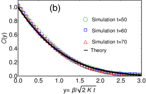
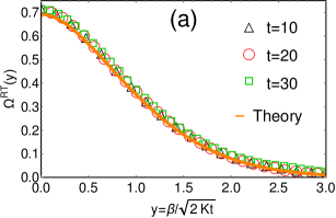
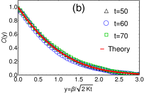
Figure 4: (a) Comparision of the scaling function Ξ©R​T​(y)superscriptΩ𝑅𝑇𝑦\Omega^{RT}(y) in Eq. (47) for run and tumble particles when tβ‰ͺ1ΞΆmuch-less-than𝑑1𝜁t\ll\frac{1}{\zeta}. Solid orange line is the result of theory in Eq. (47) while the symbols correspond to simulation at different times. We have chosen K=2,ΞΆ=0.001formulae-sequence𝐾2𝜁0.001K=2,~{}\zeta=0.001 and v0=1subscript𝑣01v_{0}=1. (b) Plot of the scaling function π’žβ€‹(y)π’žπ‘¦\mathcal{C}(y) in Eq. (51) (shown by red solid line) obtained for RTPs when t≫1ΞΆmuch-greater-than𝑑1𝜁t\gg\frac{1}{\zeta} and comparision with the numerical simulations for three different values of t𝑑t (shown by symbols). We have chosen K=2,ΞΆ=2formulae-sequence𝐾2𝜁2K=2,~{}\zeta=2 and v0=1subscript𝑣01v_{0}=1. For both (a) and (b), simulation is done with N=200𝑁200N=200 particles on a ring.

3.2 Covariance for RTP chain

We next look at the covariance for the chain of RTPs which is obtained by putting t1=t2subscript𝑑1subscript𝑑2t_{1}=t_{2} in CΞ±,Ξ²1​(t1,t2)subscriptsuperscript𝐢1𝛼𝛽subscript𝑑1subscript𝑑2C^{1}_{\alpha,\beta}(t_{1},t_{2}) in Eq. (11). In the previous section, we saw that the MSD possesses interesting scaling behaviours with repect to t𝑑t depending on where the observation time t𝑑t lies. Question is - How does CΞ±,Ξ²1​(t,t)=⟨xα​(t)​xΞ±+β​(t)⟩csubscriptsuperscript𝐢1𝛼𝛽𝑑𝑑subscriptdelimited-⟨⟩subscriptπ‘₯𝛼𝑑subscriptπ‘₯𝛼𝛽𝑑𝑐C^{1}_{\alpha,\beta}(t,t)=\langle x_{\alpha}(t)x_{\alpha+\beta}(t)\rangle_{c} behave for different regimes of t𝑑t? Before answering this question, we note that due to the translational symmetry with respect to α𝛼\alpha, ⟨xα​(t)​xΞ±+β​(t)⟩csubscriptdelimited-⟨⟩subscriptπ‘₯𝛼𝑑subscriptπ‘₯𝛼𝛽𝑑𝑐\langle x_{\alpha}(t)x_{\alpha+\beta}(t)\rangle_{c} will be independent of α𝛼\alpha. Hence without loss of generality we take Ξ±=0𝛼0\alpha=0.

Proceeding further, we use the definition of Fourier transform in Eq. (21) to write xα​(t)subscriptπ‘₯𝛼𝑑x_{\alpha}(t) in terms of xΒ―s​(t)subscriptΒ―π‘₯𝑠𝑑\bar{x}_{s}(t) which finally gives the correlation function as

⟨x0​(t)​xβ​(t)⟩cR​T​P=βˆ‘s,sβ€²=0Nβˆ’1e2​π​i​s​βNβ€‹βŸ¨xΒ―s​(t)​xΒ―sβ€²βˆ—β€‹(t)⟩cR​T​P.superscriptsubscriptdelimited-⟨⟩subscriptπ‘₯0𝑑subscriptπ‘₯𝛽𝑑𝑐𝑅𝑇𝑃superscriptsubscript𝑠superscript𝑠′0𝑁1superscript𝑒2πœ‹π‘–π‘ π›½π‘superscriptsubscriptdelimited-⟨⟩subscriptΒ―π‘₯𝑠𝑑subscriptsuperscriptΒ―π‘₯superscript𝑠′𝑑𝑐𝑅𝑇𝑃\displaystyle\langle x_{0}(t)x_{\beta}(t)\rangle_{c}^{RTP}=\sum_{s,s^{\prime}=0}^{N-1}e^{\frac{2\pi is\beta}{N}}\langle\bar{x}_{s}(t)\bar{x}^{*}_{s^{\prime}}(t)\rangle_{c}^{RTP}. (42)

Inserting ⟨xΒ―s​(t)​xΒ―sβ€²βˆ—β€‹(t)⟩cR​T​Psuperscriptsubscriptdelimited-⟨⟩subscriptΒ―π‘₯𝑠𝑑subscriptsuperscriptΒ―π‘₯superscript𝑠′𝑑𝑐𝑅𝑇𝑃\langle\bar{x}_{s}(t)\bar{x}^{*}_{s^{\prime}}(t)\rangle_{c}^{RTP} from Eq. (30) in Eq. (42), we find that the imaginary part of ⟨x0​(t)​xβ​(t)⟩csubscriptdelimited-⟨⟩subscriptπ‘₯0𝑑subscriptπ‘₯𝛽𝑑𝑐\langle x_{0}(t)x_{\beta}(t)\rangle_{c} vanishes and we get

⟨x0​(t)​xβ​(t)⟩cR​T​P=v02Nβ€‹βˆ‘s=0Nβˆ’1cos⁑(2​π​s​βN)​𝒒​(2​΢,as,t),superscriptsubscriptdelimited-⟨⟩subscriptπ‘₯0𝑑subscriptπ‘₯𝛽𝑑𝑐𝑅𝑇𝑃superscriptsubscript𝑣02𝑁superscriptsubscript𝑠0𝑁12πœ‹π‘ π›½π‘π’’2𝜁subscriptπ‘Žπ‘ π‘‘\displaystyle\langle x_{0}(t)x_{\beta}(t)\rangle_{c}^{RTP}=\frac{v_{0}^{2}}{N}\sum_{s=0}^{N-1}\cos\left(\frac{2\pi s\beta}{N}\right)\mathcal{G}(2\zeta,a_{s},t), (43)

where assubscriptπ‘Žπ‘ a_{s} and 𝒒​(2​΢,as,t)𝒒2𝜁subscriptπ‘Žπ‘ π‘‘\mathcal{G}(2\zeta,a_{s},t) are given by Eqs. (26) and (31) respectively. We first analyse Eq. (43) in the limit Nβ†’βˆžβ†’π‘N\to\infty. The finite N𝑁N case will be discussed in sec.Β 3.5. For large N𝑁N, we can change the summation to integration on the R.H.S. of Eq. (43). Changing 1Nβ€‹βˆ‘sβ†’12β€‹Ο€β€‹βˆ«βˆ’Ο€Ο€π‘‘qβ†’1𝑁subscript𝑠12πœ‹superscriptsubscriptπœ‹πœ‹differential-dπ‘ž\frac{1}{N}\sum_{s}\to\frac{1}{2\pi}\int_{-\pi}^{\pi}dq where q=2​π​sNπ‘ž2πœ‹π‘ π‘q=\frac{2\pi s}{N}, the expression of ⟨x0​(t)​xβ​(t)⟩cR​T​Psuperscriptsubscriptdelimited-⟨⟩subscriptπ‘₯0𝑑subscriptπ‘₯𝛽𝑑𝑐𝑅𝑇𝑃\langle x_{0}(t)x_{\beta}(t)\rangle_{c}^{RTP} now reads

⟨x0​(t)​xβ​(t)⟩cR​T​P≃v022β€‹Ο€β€‹βˆ«βˆ’Ο€Ο€π‘‘q​cos⁑(q​β)​𝒒​(2​΢,bq,t),similar-to-or-equalssuperscriptsubscriptdelimited-⟨⟩subscriptπ‘₯0𝑑subscriptπ‘₯𝛽𝑑𝑐𝑅𝑇𝑃superscriptsubscript𝑣022πœ‹superscriptsubscriptπœ‹πœ‹differential-dπ‘žπ‘žπ›½π’’2𝜁subscriptπ‘π‘žπ‘‘\displaystyle\langle x_{0}(t)x_{\beta}(t)\rangle_{c}^{RTP}\simeq\frac{v_{0}^{2}}{2\pi}\int_{-\pi}^{\pi}dq~{}\cos\left(q\beta\right)~{}\mathcal{G}(2\zeta,b_{q},t), (44)

where bq=4​K​sin2⁑(q/2)subscriptπ‘π‘ž4𝐾superscript2π‘ž2b_{q}=4K\sin^{2}\left(q/2\right).

As done for the MSD, we study correlations for different limits of t𝑑t. For tβ‰ͺΟ„Kmuch-less-than𝑑subscript𝜏𝐾t\ll\tau_{K}, as explained before, the motion of the two particles will be uncorrelated, hence ⟨x0​(t)​xβ​(t)⟩cR​T​P≃v02​t2​δ0,Ξ²similar-to-or-equalssuperscriptsubscriptdelimited-⟨⟩subscriptπ‘₯0𝑑subscriptπ‘₯𝛽𝑑𝑐𝑅𝑇𝑃superscriptsubscript𝑣02superscript𝑑2subscript𝛿0𝛽\langle x_{0}(t)x_{\beta}(t)\rangle_{c}^{RTP}\simeq v_{0}^{2}t^{2}~{}\delta_{0,\beta}. In the opposite limit t≫τKmuch-greater-than𝑑subscript𝜏𝐾t\gg\tau_{K} they get nontrivially correlated. As in the case of the MSD, here also, we get terms like βˆΌβˆ«π‘‘q​h​(q)​exp​[βˆ’K​t​sin2⁑(q/2)]similar-toabsentdifferential-dπ‘žβ„Žπ‘žexpdelimited-[]𝐾𝑑superscript2π‘ž2\sim\int dq~{}h(q)~{}\text{exp}\left[-Kt\sin^{2}(q/2)\right] when we insert 𝒒​(2​΢,bq,t)𝒒2𝜁subscriptπ‘π‘žπ‘‘\mathcal{G}(2\zeta,b_{q},t) from Eq. (31) in Eq. (44). In the limit K​tβ†’βˆžβ†’πΎπ‘‘Kt\to\infty, such integrals will be dominated by the small values of qπ‘žq where one can approximate bq≃K​q2similar-to-or-equalssubscriptπ‘π‘žπΎsuperscriptπ‘ž2b_{q}\simeq Kq^{2}. The details of the calculation of ⟨x0​(t)​xβ​(t)⟩cR​T​Psuperscriptsubscriptdelimited-⟨⟩subscriptπ‘₯0𝑑subscriptπ‘₯𝛽𝑑𝑐𝑅𝑇𝑃\langle x_{0}(t)x_{\beta}(t)\rangle_{c}^{RTP} for t≫τKmuch-greater-than𝑑subscript𝜏𝐾t\gg\tau_{K} is relegated to C. The final expression reads

⟨x0​(t)​xβ​(t)⟩cR​T​P≃v024​π​2​t3Kβ€‹βˆ«βˆ’βˆžβˆžπ‘‘w​cos⁑(w​β2​K​t)​𝒒​(2​΢​t,w22,1),similar-to-or-equalssuperscriptsubscriptdelimited-⟨⟩subscriptπ‘₯0𝑑subscriptπ‘₯𝛽𝑑𝑐𝑅𝑇𝑃superscriptsubscript𝑣024πœ‹2superscript𝑑3𝐾superscriptsubscriptdifferential-d𝑀𝑀𝛽2𝐾𝑑𝒒2πœπ‘‘superscript𝑀221\displaystyle\langle x_{0}(t)x_{\beta}(t)\rangle_{c}^{RTP}\simeq\frac{v_{0}^{2}}{4\pi}\sqrt{\frac{2t^{3}}{K}}\int_{-\infty}^{\infty}dw~{}\cos\left(\frac{w\beta}{\sqrt{2Kt}}\right)~{}\mathcal{G}\left(2\zeta t,\frac{w^{2}}{2},1\right), (45)

To gain more insights, we consider the expression in various limits of ΢​tπœπ‘‘\zeta t. Let us first consider ΢​tβ†’0β†’πœπ‘‘0\zeta t\to 0 limit for which we use Eq. (31) to approximate 𝒒​(2​΢​tβ†’0,w22,1)≃4​(1βˆ’eβˆ’w22w2)2similar-to-or-equals𝒒→2πœπ‘‘0superscript𝑀2214superscript1superscript𝑒superscript𝑀22superscript𝑀22\mathcal{G}\left(2\zeta t\to 0,\frac{w^{2}}{2},1\right)\simeq 4\left(\frac{1-e^{-\frac{w^{2}}{2}}}{w^{2}}\right)^{2}. Substituting this form of 𝒒​(2​΢​t,w22,1)𝒒2πœπ‘‘superscript𝑀221\mathcal{G}\left(2\zeta t,\frac{w^{2}}{2},1\right) in the R.H.S. of Eq. (45) and performing the integration over w𝑀w, we find that ⟨x0​(t)​xβ​(t)⟩cR​T​Psuperscriptsubscriptdelimited-⟨⟩subscriptπ‘₯0𝑑subscriptπ‘₯𝛽𝑑𝑐𝑅𝑇𝑃\langle x_{0}(t)x_{\beta}(t)\rangle_{c}^{RTP} obeys the scaling form

⟨x0​(t)​xβ​(t)⟩cR​T​P≃v02π​2​t3K​ΩR​T​(Ξ²2​K​t),for ​τKβ‰ͺtβ‰ͺ1ΞΆ,formulae-sequencesimilar-to-or-equalssuperscriptsubscriptdelimited-⟨⟩subscriptπ‘₯0𝑑subscriptπ‘₯𝛽𝑑𝑐𝑅𝑇𝑃superscriptsubscript𝑣02πœ‹2superscript𝑑3𝐾superscriptΩ𝑅𝑇𝛽2𝐾𝑑much-less-thanforΒ subscriptπœπΎπ‘‘much-less-than1𝜁\displaystyle\langle x_{0}(t)x_{\beta}(t)\rangle_{c}^{RTP}\simeq\frac{v_{0}^{2}}{\pi}\sqrt{\frac{2t^{3}}{K}}~{}\Omega^{RT}\left(\frac{\beta}{\sqrt{2Kt}}\right),~{}~{}~{}~{}~{}~{}~{}\text{for }\tau_{K}\ll t\ll\frac{1}{\zeta}, (46)

where the scaling function Ξ©R​T​(y)superscriptΩ𝑅𝑇𝑦\Omega^{RT}(y) is given as

Ξ©R​T​(y)=Ο€6[2eβˆ’y24(4+y2)βˆ’22eβˆ’y22(2+y2)βˆ’Ο€y(6+y2)Erfc(y2)+2Ο€y(3+y2)Erfc(y2)].superscriptΞ©π‘…π‘‡π‘¦πœ‹6delimited-[]2superscript𝑒superscript𝑦244superscript𝑦222superscript𝑒superscript𝑦222superscript𝑦2πœ‹π‘¦6superscript𝑦2Erfc𝑦22πœ‹π‘¦3superscript𝑦2Erfc𝑦2\displaystyle\begin{split}\Omega^{RT}(y)=&\frac{\sqrt{\pi}}{6}\left[2e^{-\frac{y^{2}}{4}}\left(4+y^{2}\right)-2\sqrt{2}e^{-\frac{y^{2}}{2}}\left(2+y^{2}\right)\right.\\ &\left.-\sqrt{\pi}y(6+y^{2})~{}\text{Erfc}\left(\frac{y}{2}\right)+2\sqrt{\pi}y(3+y^{2})~{}\text{Erfc}\left(\frac{y}{\sqrt{2}}\right)\right].\end{split} (47)

In Figure 4(a) we have plotted Ξ©R​T​(y)superscriptΩ𝑅𝑇𝑦\Omega^{RT}(y) and compared with the results of numerical simulations for three different times. For all values of t𝑑t in range Ο„Kβ‰ͺtβ‰ͺ1ΞΆmuch-less-thansubscriptπœπΎπ‘‘much-less-than1𝜁\tau_{K}\ll t\ll\frac{1}{\zeta}, the simulation data collapse over our theoretical result in Eq. (47). The scaling function Ξ©R​T​(y)superscriptΩ𝑅𝑇𝑦\Omega^{RT}(y) has the following asymptotic forms:

Ξ©R​T​(y)superscriptΩ𝑅𝑇𝑦\displaystyle\Omega^{RT}(y) ≃2​π3​(2βˆ’2)βˆ’Ο€β€‹(2βˆ’1)​y2+O​(y3),as ​yβ†’0,formulae-sequencesimilar-to-or-equalsabsent2πœ‹322πœ‹21superscript𝑦2𝑂superscript𝑦3β†’as 𝑦0\displaystyle\simeq\frac{2\sqrt{\pi}}{3}(2-\sqrt{2}){-\sqrt{\pi}\left(\sqrt{2}-1\right)y^{2}+O(y^{3})},~{}~{}~{}~{}~{}~{}~{}\text{as }y\to 0, (48)
≃(2​πy4+O​(yβˆ’6))​eβˆ’y24,as ​yβ†’βˆž.formulae-sequencesimilar-to-or-equalsabsent2πœ‹superscript𝑦4𝑂superscript𝑦6superscript𝑒superscript𝑦24β†’as 𝑦\displaystyle\simeq\left(\frac{2\sqrt{\pi}}{y^{4}}+O\left(y^{-6}\right)\right)e^{-\frac{y^{2}}{4}},~{}~{}~{}~{}~{}~{}~{}~{}~{}~{}~{}~{}~{}~{}~{}~{}~{}~{}~{}~{}~{}~{}~{}~{}~{}~{}~{}\text{as }y\to\infty. (49)

Inserting the asymptotic form of Ξ©R​T​(y)superscriptΩ𝑅𝑇𝑦\Omega^{RT}(y) for large y𝑦y, one finds that ⟨x0​(t)​xβ​(t)⟩cR​T​Psuperscriptsubscriptdelimited-⟨⟩subscriptπ‘₯0𝑑subscriptπ‘₯𝛽𝑑𝑐𝑅𝑇𝑃\langle x_{0}(t)x_{\beta}(t)\rangle_{c}^{RTP} in Eq. (46) has faster than exponential decay for large β𝛽\beta (≫K​tmuch-greater-thanabsent𝐾𝑑\gg\sqrt{Kt}) with a decay length ld=2​2​K​tsubscript𝑙𝑑22𝐾𝑑l_{d}=2\sqrt{2Kt}. On the other hand, for Ξ²β†’0→𝛽0\beta\to 0, ⟨x0​(t)​xβ​(t)⟩cR​T​Psuperscriptsubscriptdelimited-⟨⟩subscriptπ‘₯0𝑑subscriptπ‘₯𝛽𝑑𝑐𝑅𝑇𝑃\langle x_{0}(t)x_{\beta}(t)\rangle_{c}^{RTP} correctly reduces to the MSD obtained in Eq. (40).

Let us now consider the opposite limit ΢​tβ†’βˆžβ†’πœπ‘‘\zeta t\to\infty for ⟨x0​(t)​xβ​(t)⟩cR​T​Psuperscriptsubscriptdelimited-⟨⟩subscriptπ‘₯0𝑑subscriptπ‘₯𝛽𝑑𝑐𝑅𝑇𝑃\langle x_{0}(t)x_{\beta}(t)\rangle_{c}^{RTP} in Eq. (45). In this limit, from Eq. (31), we get 𝒒​(2​΢​tβ†’βˆž,w22,1)≃1βˆ’eβˆ’w2΢​t​w2similar-to-or-equals𝒒→2πœπ‘‘superscript𝑀2211superscript𝑒superscript𝑀2πœπ‘‘superscript𝑀2\mathcal{G}\left(2\zeta t\to\infty,\frac{w^{2}}{2},1\right)\simeq\frac{1-e^{-w^{2}}}{\zeta tw^{2}} which can be used in Eq. (45) to obtain the scaling form

⟨x0​(t)​xβ​(t)⟩cR​T​P≃DR​2​tπ​Kβ€‹π’žβ€‹(Ξ²2​K​t),for ​t≫1ΞΆ,formulae-sequencesimilar-to-or-equalssuperscriptsubscriptdelimited-⟨⟩subscriptπ‘₯0𝑑subscriptπ‘₯𝛽𝑑𝑐𝑅𝑇𝑃subscript𝐷𝑅2π‘‘πœ‹πΎπ’žπ›½2𝐾𝑑much-greater-thanfor 𝑑1𝜁\displaystyle\langle x_{0}(t)x_{\beta}(t)\rangle_{c}^{RTP}\simeq D_{R}\sqrt{\frac{2t}{\pi K}}~{}\mathcal{C}\left(\frac{\beta}{\sqrt{2Kt}}\right),~{}~{}~{}~{}~{}~{}~{}\text{for }t\gg\frac{1}{\zeta}, (50)

where DR=v022​΢subscript𝐷𝑅superscriptsubscript𝑣022𝜁D_{R}=\frac{v_{0}^{2}}{2\zeta} and the scaling function π’žβ€‹(y)π’žπ‘¦\mathcal{C}(y) is given by

π’žβ€‹(y)=eβˆ’y24βˆ’Ο€2​y​Erfc​(y2).π’žπ‘¦superscript𝑒superscript𝑦24πœ‹2𝑦Erfc𝑦2\displaystyle\mathcal{C}(y)=e^{-\frac{y^{2}}{4}}-\frac{\sqrt{\pi}}{2}y~{}\text{Erfc}\left(\frac{y}{2}\right). (51)

Same scaling form for the correlation function has been observed in the context of single file problems in random average process [20, 21, 18] and in symmetric exclusion process [22, 23]. In Figure 4(b), we have plotted and compared π’žβ€‹(y)π’žπ‘¦\mathcal{C}(y) with the numerical simulations for three different values of t𝑑t for ΞΆ=2𝜁2\zeta=2. We observe an excellent agreement of the theoretical result with the simulation results for all t𝑑t. The scaling function π’žβ€‹(y)π’žπ‘¦\mathcal{C}(y) has the following asymptotic forms;

π’žβ€‹(y)π’žπ‘¦\displaystyle\mathcal{C}(y) ≃1βˆ’Ο€2​y,as ​yβ†’0,formulae-sequencesimilar-to-or-equalsabsent1πœ‹2𝑦→as 𝑦0\displaystyle\simeq 1-{\frac{\sqrt{\pi}}{2}y},~{}~{}~{}~{}~{}~{}~{}~{}~{}~{}~{}~{}~{}~{}~{}~{}~{}~{}~{}~{}~{}~{}~{}\text{as }y\to 0, (52)
≃(2y2+O​(yβˆ’4))​eβˆ’y24,as ​yβ†’βˆž.formulae-sequencesimilar-to-or-equalsabsent2superscript𝑦2𝑂superscript𝑦4superscript𝑒superscript𝑦24β†’as 𝑦\displaystyle\simeq{\left(\frac{2}{y^{2}}+O\left(y^{-4}\right)\right)e^{-\frac{y^{2}}{4}},}~{}~{}~{}~{}~{}~{}~{}\text{as }y\to\infty. (53)

Again, for Ξ²β†’0→𝛽0\beta\to 0, the scaling form in Eq. (50) correctly reduces to the MSD in Eq. (41) for t≫1ΞΆmuch-greater-than𝑑1𝜁t\gg\frac{1}{\zeta}. Also, ⟨x0​(t)​xβ​(t)⟩cR​T​Psuperscriptsubscriptdelimited-⟨⟩subscriptπ‘₯0𝑑subscriptπ‘₯𝛽𝑑𝑐𝑅𝑇𝑃\langle x_{0}(t)x_{\beta}(t)\rangle_{c}^{RTP} has faster than exponential decay for large β𝛽\beta (≫K​tmuch-greater-thanabsent𝐾𝑑\gg\sqrt{Kt}) with a decay length ld=2​2​K​tsubscript𝑙𝑑22𝐾𝑑l_{d}=2\sqrt{2Kt}.

Refer to caption
Refer to caption
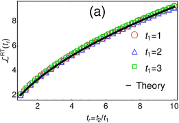
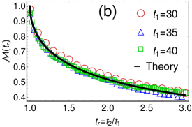
Figure 5: Illustration of the scaling forms obtained in (60) and (66) for ⟨xα​(t1)​xα​(t2)⟩cR​T​Psuperscriptsubscriptdelimited-⟨⟩subscriptπ‘₯𝛼subscript𝑑1subscriptπ‘₯𝛼subscript𝑑2𝑐𝑅𝑇𝑃\langle x_{\alpha}(t_{1})x_{\alpha}(t_{2})\rangle_{c}^{RTP} for t≫1ΞΆmuch-greater-than𝑑1𝜁t\gg\frac{1}{\zeta} and tβ‰ͺ1ΞΆmuch-less-than𝑑1𝜁t\ll\frac{1}{\zeta} respectively. In both (a) and (b), the black solid line is the analytical result while symbols correspond to the simulation data for different values of t1subscript𝑑1t_{1}. We have taken ΞΆ=0.001𝜁0.001\zeta=0.001 for plot (a) and ΞΆ=2𝜁2\zeta=2 for plot (b). For both plots, simulation is done for N=200𝑁200N=200 particles with K=3𝐾3K=3 and v0=1subscript𝑣01v_{0}=1.

3.3 Position auto correlation for RTP chain

We next study the position auto correlation ⟨xα​(t1)​xα​(t2)⟩csubscriptdelimited-⟨⟩subscriptπ‘₯𝛼subscript𝑑1subscriptπ‘₯𝛼subscript𝑑2𝑐\langle x_{\alpha}(t_{1})x_{\alpha}(t_{2})\rangle_{c} between the positions of a tagged particle (say α𝛼\alphath) at times t1subscript𝑑1t_{1} and t2subscript𝑑2t_{2}. The translational symmetry in α𝛼\alpha makes ⟨xα​(t1)​xα​(t2)⟩csubscriptdelimited-⟨⟩subscriptπ‘₯𝛼subscript𝑑1subscriptπ‘₯𝛼subscript𝑑2𝑐\langle x_{\alpha}(t_{1})x_{\alpha}(t_{2})\rangle_{c} independent of α𝛼\alpha. Also without loss of generality, we assume t1≀t2subscript𝑑1subscript𝑑2t_{1}\leq t_{2} throughout our analysis. To proceed further, we insert the unequal time correlations of FΒ―sR​T​P​(t)subscriptsuperscript¯𝐹𝑅𝑇𝑃𝑠𝑑\bar{F}^{RTP}_{s}(t) derived in Eqs. (167) in xΒ―s​(t)subscriptΒ―π‘₯𝑠𝑑\bar{x}_{s}(t) in Eq. (27) to yield

⟨xΒ―s​(t1)​xΒ―sβ€²βˆ—β€‹(t2)⟩cR​T​P=Ξ΄s,s′​v02N​ℋ​(2​΢,as,t1,t2),superscriptsubscriptdelimited-⟨⟩subscriptΒ―π‘₯𝑠subscript𝑑1superscriptsubscriptΒ―π‘₯superscript𝑠′subscript𝑑2𝑐𝑅𝑇𝑃subscript𝛿𝑠superscript𝑠′superscriptsubscript𝑣02𝑁ℋ2𝜁subscriptπ‘Žπ‘ subscript𝑑1subscript𝑑2\displaystyle\langle\bar{x}_{s}(t_{1})\bar{x}_{s^{\prime}}^{*}(t_{2})\rangle_{c}^{RTP}~{}=\delta_{s,s^{\prime}}~{}\frac{v_{0}^{2}}{N}\mathcal{H}\left(2\zeta,a_{s},t_{1},t_{2}\right), (54)

where assubscriptπ‘Žπ‘ a_{s} is given in Eq. (26) and the function ℋ​(a,b,t1,t2)β„‹π‘Žπ‘subscript𝑑1subscript𝑑2\mathcal{H}(a,b,t_{1},t_{2}) is

ℋ​(a,b,t1,t2)=βˆ’ab​eβˆ’b​|t1βˆ’t2|βˆ’eβˆ’b​(t1+t2)(b2βˆ’a2)+eβˆ’a​|t1βˆ’t2|βˆ’eβˆ’(b​t1+a​t2)(b2βˆ’a2)βˆ’eβˆ’(a​t1+b​t2)βˆ’eβˆ’b​(t1+t2)(b2βˆ’a2)β„‹π‘Žπ‘subscript𝑑1subscript𝑑2π‘Žπ‘superscript𝑒𝑏subscript𝑑1subscript𝑑2superscript𝑒𝑏subscript𝑑1subscript𝑑2superscript𝑏2superscriptπ‘Ž2superscriptπ‘’π‘Žsubscript𝑑1subscript𝑑2superscript𝑒𝑏subscript𝑑1π‘Žsubscript𝑑2superscript𝑏2superscriptπ‘Ž2superscriptπ‘’π‘Žsubscript𝑑1𝑏subscript𝑑2superscript𝑒𝑏subscript𝑑1subscript𝑑2superscript𝑏2superscriptπ‘Ž2\displaystyle\begin{split}\mathcal{H}(a,b,t_{1},t_{2})=&-\frac{a}{b}\frac{e^{-b|t_{1}-t_{2}|}-e^{-b(t_{1}+t_{2})}}{(b^{2}-a^{2})}+\frac{e^{-a|t_{1}-t_{2}|}-e^{-(bt_{1}+at_{2})}}{(b^{2}-a^{2})}\\ &~{}~{}~{}~{}~{}~{}~{}~{}~{}~{}~{}~{}~{}~{}~{}-\frac{e^{-(at_{1}+bt_{2})}-e^{-b(t_{1}+t_{2})}}{(b^{2}-a^{2})}\end{split} (55)

The correlation function ⟨xΒ―s​(t1)​xΒ―s′​(t2)⟩csubscriptdelimited-⟨⟩subscriptΒ―π‘₯𝑠subscript𝑑1subscriptΒ―π‘₯superscript𝑠′subscript𝑑2𝑐\langle\bar{x}_{s}(t_{1})\bar{x}_{s^{\prime}}(t_{2})\rangle_{c} can be easily translated to ⟨xα​(t1)​xα​(t2)⟩csubscriptdelimited-⟨⟩subscriptπ‘₯𝛼subscript𝑑1subscriptπ‘₯𝛼subscript𝑑2𝑐\langle x_{\alpha}(t_{1})x_{\alpha}(t_{2})\rangle_{c} by writing xα​(t)subscriptπ‘₯𝛼𝑑x_{\alpha}(t) in terms of xΒ―s​(t)subscriptΒ―π‘₯𝑠𝑑\bar{x}_{s}(t) from Eq. (21). Finally, we get

⟨xα​(t1)​xα​(t2)⟩cR​T​Psuperscriptsubscriptdelimited-⟨⟩subscriptπ‘₯𝛼subscript𝑑1subscriptπ‘₯𝛼subscript𝑑2𝑐𝑅𝑇𝑃\displaystyle\langle x_{\alpha}(t_{1})x_{\alpha}(t_{2})\rangle_{c}^{RTP} =βˆ‘sβ€²,s=0Nβˆ’1⟨xΒ―s​(t1)​xΒ―sβ€²βˆ—β€‹(t2)⟩cR​T​P,absentsuperscriptsubscriptsuperscript𝑠′𝑠0𝑁1superscriptsubscriptdelimited-⟨⟩subscriptΒ―π‘₯𝑠subscript𝑑1superscriptsubscriptΒ―π‘₯superscript𝑠′subscript𝑑2𝑐𝑅𝑇𝑃\displaystyle=\sum_{s^{\prime},s=0}^{N-1}\langle\bar{x}_{s}(t_{1})\bar{x}_{s^{\prime}}^{*}(t_{2})\rangle_{c}^{RTP}, (56)
=v02Nβ€‹βˆ‘s=0Nβˆ’1ℋ​(2​΢,as,t1,t2),absentsuperscriptsubscript𝑣02𝑁superscriptsubscript𝑠0𝑁1β„‹2𝜁subscriptπ‘Žπ‘ subscript𝑑1subscript𝑑2\displaystyle=\frac{v_{0}^{2}}{N}\sum_{s=0}^{N-1}\mathcal{H}\left(2\zeta,a_{s},t_{1},t_{2}\right), (57)

As we show later, for this case also, one can obtain various interesting scaling forms and scaling functions in the limit Nβ†’βˆžβ†’π‘N\to\infty. Changing the summation in the R.H.S. of Eq. (57) to the integration as 1Nβ€‹βˆ‘sβ†’12β€‹Ο€β€‹βˆ«βˆ’Ο€Ο€π‘‘qβ†’1𝑁subscript𝑠12πœ‹superscriptsubscriptπœ‹πœ‹differential-dπ‘ž\frac{1}{N}\sum_{s}\to\frac{1}{2\pi}\int_{-\pi}^{\pi}dq in Eq.Β (57) with q=2​π​sNπ‘ž2πœ‹π‘ π‘q=\frac{2\pi s}{N}, we get

⟨xα​(t1)​xα​(t2)⟩cR​T​P≃v022β€‹Ο€β€‹βˆ«βˆ’Ο€Ο€π‘‘q​ℋ​(2​΢,bq,t1,t2).similar-to-or-equalssuperscriptsubscriptdelimited-⟨⟩subscriptπ‘₯𝛼subscript𝑑1subscriptπ‘₯𝛼subscript𝑑2𝑐𝑅𝑇𝑃superscriptsubscript𝑣022πœ‹superscriptsubscriptπœ‹πœ‹differential-dπ‘žβ„‹2𝜁subscriptπ‘π‘žsubscript𝑑1subscript𝑑2\displaystyle\langle x_{\alpha}(t_{1})x_{\alpha}(t_{2})\rangle_{c}^{RTP}\simeq\frac{v_{0}^{2}}{2\pi}\int_{-\pi}^{\pi}dq~{}\mathcal{H}\left(2\zeta,b_{q},t_{1},t_{2}\right). (58)

Here bq=4​K​sin2⁑(q/2)subscriptπ‘π‘ž4𝐾superscript2π‘ž2b_{q}=4K\sin^{2}(q/2). We now look at this expression in various limits of t1subscript𝑑1t_{1} with respect to Ο„Ksubscript𝜏𝐾\tau_{K} keeping the ratio t2t1subscript𝑑2subscript𝑑1\frac{t_{2}}{t_{1}} fixed. We again emphasise that we consider t1≀t2subscript𝑑1subscript𝑑2t_{1}\leq t_{2}.

We begin with the case when t1β‰ͺΟ„Kmuch-less-thansubscript𝑑1subscript𝜏𝐾t_{1}\ll\tau_{K} and t2β‰ͺΟ„Kmuch-less-thansubscript𝑑2subscript𝜏𝐾t_{2}\ll\tau_{K} while keeping the ratio t2t1subscript𝑑2subscript𝑑1\frac{t_{2}}{t_{1}} is fixed. Recall that Ο„Ksubscript𝜏𝐾\tau_{K} is the smallest time scale in the model (see Fig. 2) which means that t1subscript𝑑1t_{1} and t2subscript𝑑2t_{2} are smaller than all the time scales present in the model in this case. At this small time scale, the particle moves ballistically and independently. As a result, we expect ⟨xα​(t1)​xα​(t2)⟩cR​T​Psuperscriptsubscriptdelimited-⟨⟩subscriptπ‘₯𝛼subscript𝑑1subscriptπ‘₯𝛼subscript𝑑2𝑐𝑅𝑇𝑃\langle x_{\alpha}(t_{1})x_{\alpha}(t_{2})\rangle_{c}^{RTP} which can be easily shown by putting ℋ​(2​΢,bq,t1,t2)≃t1​t2similar-to-or-equalsβ„‹2𝜁subscriptπ‘π‘žsubscript𝑑1subscript𝑑2subscript𝑑1subscript𝑑2\mathcal{H}\left(2\zeta,b_{q},t_{1},t_{2}\right)\simeq t_{1}t_{2} in Eq. (58) and then performing the integration over qπ‘žq.

Refer to caption
Refer to caption
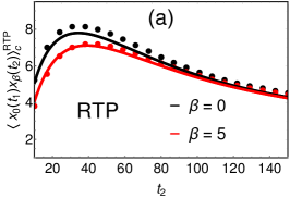
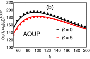
Figure 6: Non-monotonous behaviour of ⟨x0​(t1)​xβ​(t2)⟩csubscriptdelimited-⟨⟩subscriptπ‘₯0subscript𝑑1subscriptπ‘₯𝛽subscript𝑑2𝑐\langle x_{0}(t_{1})x_{\beta}(t_{2})\rangle_{c} for RTP (left panel) and AOUP (right panel). In panel (a), the analytic result (shown by solid lines) of Eq. (74) is compared against the results of simulations (shown by filled circles). We have chosen K=3,ΞΆ=0.02,v0=1,N=200,t1=10formulae-sequence𝐾3formulae-sequence𝜁0.02formulae-sequencesubscript𝑣01formulae-sequence𝑁200subscript𝑑110K=3,~{}\zeta=0.02,~{}v_{0}=1,~{}N=200,~{}t_{1}=10. In panel (b), same is done for AOUP (Eq. (103)) with D=0.1,K=2,Ξ³=0.02,N=100,t1=50formulae-sequence𝐷0.1formulae-sequence𝐾2formulae-sequence𝛾0.02formulae-sequence𝑁100subscript𝑑150D=0.1,~{}K=2,~{}\gamma=0.02,~{}N=100,~{}t_{1}=50.

Let us now consider the other limit when t1≫τKmuch-greater-thansubscript𝑑1subscript𝜏𝐾t_{1}\gg\tau_{K} and t2t1subscript𝑑2subscript𝑑1\frac{t_{2}}{t_{1}} is kept fixed. For this case also, when we insert the explicit form of ℋ​(2​΢,bq,t1,t2)β„‹2𝜁subscriptπ‘π‘žsubscript𝑑1subscript𝑑2\mathcal{H}(2\zeta,b_{q},t_{1},t_{2}) from Eq. (55) in ⟨xα​(t1)​xα​(t2)⟩cR​T​Psuperscriptsubscriptdelimited-⟨⟩subscriptπ‘₯𝛼subscript𝑑1subscriptπ‘₯𝛼subscript𝑑2𝑐𝑅𝑇𝑃\langle x_{\alpha}(t_{1})x_{\alpha}(t_{2})\rangle_{c}^{RTP} in Eq. (58), we get terms of the form βˆΌβˆ«π‘‘q​h​(q)​eβˆ’k​t​sin2⁑(q/2)similar-toabsentdifferential-dπ‘žβ„Žπ‘žsuperscriptπ‘’π‘˜π‘‘superscript2π‘ž2\sim\int dq~{}h(q)~{}e^{-kt\sin^{2}(q/2)} where h​(q)β„Žπ‘žh(q) is some function of qπ‘žq. For K​t1𝐾subscript𝑑1Kt_{1} very large, such integrals will be dominated by the small values of qπ‘žq which suggests us to approximate bq≃K​q2similar-to-or-equalssubscriptπ‘π‘žπΎsuperscriptπ‘ž2b_{q}\simeq Kq^{2} as before. Making this approximation, we find

⟨xα​(t1)​xα​(t2)⟩cR​T​P≃v022​π​t13Kβ€‹βˆ«βˆ’βˆžβˆžπ‘‘w​ℋ​(2​΢​t1,w2,1,t2t1),for ​t1≫τK.formulae-sequencesimilar-to-or-equalssuperscriptsubscriptdelimited-⟨⟩subscriptπ‘₯𝛼subscript𝑑1subscriptπ‘₯𝛼subscript𝑑2𝑐𝑅𝑇𝑃superscriptsubscript𝑣022πœ‹superscriptsubscript𝑑13𝐾superscriptsubscriptdifferential-d𝑀ℋ2𝜁subscript𝑑1superscript𝑀21subscript𝑑2subscript𝑑1much-greater-thanforΒ subscript𝑑1subscript𝜏𝐾\displaystyle\langle x_{\alpha}(t_{1})x_{\alpha}(t_{2})\rangle_{c}^{RTP}\simeq\frac{v_{0}^{2}}{2\pi}\sqrt{\frac{t_{1}^{3}}{K}}\int_{-\infty}^{\infty}dw~{}\mathcal{H}\left(2\zeta t_{1},w^{2},1,\frac{t_{2}}{t_{1}}\right),~{}~{}~{}~{}~{}~{}\text{for }t_{1}\gg\tau_{K}. (59)

We emphasise that this equation is derived assuming the ratio t2t1subscript𝑑2subscript𝑑1\frac{t_{2}}{t_{1}} is fixed. To decipher interesting scaling forms, we evaluate this equation in various limits of ΢​t1𝜁subscript𝑑1\zeta t_{1}. For ΢​t1β†’0β†’πœsubscript𝑑10\zeta t_{1}\to 0, we obtain, using the definition of β„‹β„‹\mathcal{H} in Eq. (55), that ℋ​(2​΢​t1β†’0,w2,1,tr)≃eβˆ’w2​(1+tr)​(etr​w2βˆ’1)​(ew2βˆ’1)w4similar-to-or-equalsβ„‹β†’2𝜁subscript𝑑10superscript𝑀21subscriptπ‘‘π‘Ÿsuperscript𝑒superscript𝑀21subscriptπ‘‘π‘Ÿsuperscript𝑒subscriptπ‘‘π‘Ÿsuperscript𝑀21superscript𝑒superscript𝑀21superscript𝑀4\mathcal{H}\left(2\zeta t_{1}\to 0,w^{2},1,t_{r}\right)\simeq~{}e^{-w^{2}(1+t_{r})}\frac{(e^{t_{r}w^{2}}-1)(e^{w^{2}}-1)}{w^{4}} where tr=t2/t1subscriptπ‘‘π‘Ÿsubscript𝑑2subscript𝑑1t_{r}=t_{2}/t_{1}. Putting this expression in Eq. (59) and performing the integration over w𝑀w, we obtain that ⟨xα​(t1)​xα​(t2)⟩cR​T​Psuperscriptsubscriptdelimited-⟨⟩subscriptπ‘₯𝛼subscript𝑑1subscriptπ‘₯𝛼subscript𝑑2𝑐𝑅𝑇𝑃\langle x_{\alpha}(t_{1})x_{\alpha}(t_{2})\rangle_{c}^{RTP} has the scaling form

⟨xα​(t1)​xα​(t2)⟩cR​T​Psuperscriptsubscriptdelimited-⟨⟩subscriptπ‘₯𝛼subscript𝑑1subscriptπ‘₯𝛼subscript𝑑2𝑐𝑅𝑇𝑃\displaystyle\langle x_{\alpha}(t_{1})x_{\alpha}(t_{2})\rangle_{c}^{RTP} ≃v022​π​t13K​ℒR​T​(t2t1),for ​τKβ‰ͺt1<t2β‰ͺ1ΞΆ,formulae-sequencesimilar-to-or-equalsabsentsuperscriptsubscript𝑣022πœ‹superscriptsubscript𝑑13𝐾superscriptℒ𝑅𝑇subscript𝑑2subscript𝑑1much-less-thanforΒ subscript𝜏𝐾subscript𝑑1subscript𝑑2much-less-than1𝜁\displaystyle\simeq\frac{v_{0}^{2}}{2\pi}\sqrt{\frac{t_{1}^{3}}{K}}~{}\mathcal{L}^{RT}\left(\frac{t_{2}}{t_{1}}\right),~{}~{}~{}~{}{\text{for }\tau_{K}\ll t_{1}<t_{2}\ll\frac{1}{\zeta}}, (60)

with the scaling function β„’R​T​(tr)superscriptℒ𝑅𝑇subscriptπ‘‘π‘Ÿ\mathcal{L}^{RT}(t_{r}) given by

β„’R​T​(tr)=4​π3​[(1+tr)3/2βˆ’1βˆ’tr3/2].superscriptℒ𝑅𝑇subscriptπ‘‘π‘Ÿ4πœ‹3delimited-[]superscript1subscriptπ‘‘π‘Ÿ321superscriptsubscriptπ‘‘π‘Ÿ32\displaystyle\mathcal{L}^{RT}(t_{r})=\frac{4\sqrt{\pi}}{3}\left[(1+t_{r})^{3/2}-1-t_{r}^{3/2}\right]. (61)

In Fig.Β 5(a), we have presented the comparision of our analytic result with the same obtained from the numerical simulation. We have considered three different values of t1subscript𝑑1t_{1} and for each t1subscript𝑑1t_{1}, we vary t2subscript𝑑2t_{2}. All simulation results match with the analytic result. The asymptotic forms of β„’R​T​(tr)superscriptℒ𝑅𝑇subscriptπ‘‘π‘Ÿ\mathcal{L}^{RT}(t_{r}) read

β„’R​T​(tr)superscriptℒ𝑅𝑇subscriptπ‘‘π‘Ÿ\displaystyle\mathcal{L}^{RT}(t_{r}) ≃8​π3​(2βˆ’1)+2​π​(2βˆ’1)​(trβˆ’1),as ​trβ†’1,formulae-sequencesimilar-to-or-equalsabsent8πœ‹3212πœ‹21subscriptπ‘‘π‘Ÿ1β†’asΒ subscriptπ‘‘π‘Ÿ1\displaystyle\simeq\frac{8\sqrt{\pi}}{3}\left(\sqrt{2}-1\right){+2\sqrt{\pi}\left(\sqrt{2}-1\right)(t_{r}-1)},~{}~{}~{}~{}~{}~{}~{}\text{as }t_{r}\to 1, (62)
≃2​π​trβˆ’4​π3,as ​tr≫1,formulae-sequencesimilar-to-or-equalsabsent2πœ‹subscriptπ‘‘π‘Ÿ4πœ‹3much-greater-thanasΒ subscriptπ‘‘π‘Ÿ1\displaystyle\simeq 2\sqrt{\pi t_{r}}-\frac{4\sqrt{\pi}}{3},~{}~{}~{}~{}~{}~{}~{}~{}~{}~{}~{}~{}~{}~{}~{}~{}~{}~{}~{}~{}~{}~{}~{}~{}~{}~{}~{}~{}~{}~{}~{}~{}~{}~{}~{}~{}~{}~{}~{}~{}~{}\text{as }{t_{r}\gg 1}, (63)

inserting which in Eq. (60), we find that the correlation ⟨xα​(t1)​xα​(t2)⟩cR​T​Psuperscriptsubscriptdelimited-⟨⟩subscriptπ‘₯𝛼subscript𝑑1subscriptπ‘₯𝛼subscript𝑑2𝑐𝑅𝑇𝑃\langle x_{\alpha}(t_{1})x_{\alpha}(t_{2})\rangle_{c}^{RTP} crosses over from t23/2superscriptsubscript𝑑232t_{2}^{3/2} behaviour to the t2subscript𝑑2\sqrt{t_{2}} behaviour as

⟨xα​(t1)​xα​(t2)⟩cR​T​Psuperscriptsubscriptdelimited-⟨⟩subscriptπ‘₯𝛼subscript𝑑1subscriptπ‘₯𝛼subscript𝑑2𝑐𝑅𝑇𝑃\displaystyle\langle x_{\alpha}(t_{1})x_{\alpha}(t_{2})\rangle_{c}^{RTP} ≃4​(2βˆ’1)3​π​K​v02​t132+O​(t2βˆ’t1),for ​t2β†’t1,formulae-sequencesimilar-to-or-equalsabsent4213πœ‹πΎsuperscriptsubscript𝑣02superscriptsubscript𝑑132𝑂subscript𝑑2subscript𝑑1β†’forΒ subscript𝑑2subscript𝑑1\displaystyle\simeq\frac{4(\sqrt{2}-1)}{3\sqrt{\pi K}}v_{0}^{2}~{}t_{1}^{\frac{3}{2}}+O\left(t_{2}-t_{1}\right),~{}~{}~{}~{}~{}~{}~{}~{}\text{for }t_{2}\to t_{1}, (64)
≃v02​t1π​K​(t2βˆ’23​t1),for ​t2≫t1.formulae-sequencesimilar-to-or-equalsabsentsuperscriptsubscript𝑣02subscript𝑑1πœ‹πΎsubscript𝑑223subscript𝑑1much-greater-thanforΒ subscript𝑑2subscript𝑑1\displaystyle\simeq\frac{v_{0}^{2}t_{1}}{\sqrt{\pi K}}\left(\sqrt{t_{2}}-\frac{2}{3}\sqrt{t_{1}}\right),~{}~{}~{}~{}~{}~{}~{}~{}~{}~{}~{}~{}~{}~{}~{}~{}~{}\text{for }t_{2}\gg t_{1}. (65)

For t1=t2subscript𝑑1subscript𝑑2t_{1}=t_{2}, ⟨xα​(t1)​xα​(t2)⟩cR​T​Psuperscriptsubscriptdelimited-⟨⟩subscriptπ‘₯𝛼subscript𝑑1subscriptπ‘₯𝛼subscript𝑑2𝑐𝑅𝑇𝑃\langle x_{\alpha}(t_{1})x_{\alpha}(t_{2})\rangle_{c}^{RTP} correctly reduces to the expression of MSD in Eq. (40). Quite remarkably, for t2≫t1much-greater-thansubscript𝑑2subscript𝑑1t_{2}\gg t_{1}, ⟨xα​(t1)​xα​(t2)⟩cR​T​Psuperscriptsubscriptdelimited-⟨⟩subscriptπ‘₯𝛼subscript𝑑1subscriptπ‘₯𝛼subscript𝑑2𝑐𝑅𝑇𝑃\langle x_{\alpha}(t_{1})x_{\alpha}(t_{2})\rangle_{c}^{RTP} increases with increasing t2subscript𝑑2t_{2} while both t1subscript𝑑1t_{1} and t2subscript𝑑2t_{2} being smaller than Ο„Asubscript𝜏𝐴\tau_{A}.

We next look at ⟨xα​(t1)​xα​(t2)⟩cR​T​Psuperscriptsubscriptdelimited-⟨⟩subscriptπ‘₯𝛼subscript𝑑1subscriptπ‘₯𝛼subscript𝑑2𝑐𝑅𝑇𝑃\langle x_{\alpha}(t_{1})x_{\alpha}(t_{2})\rangle_{c}^{RTP} in the other limit ΢​t1β†’βˆžβ†’πœsubscript𝑑1\zeta t_{1}\to\infty while the ratio t2/t1subscript𝑑2subscript𝑑1t_{2}/t_{1} is again held fixed. In this limit, we use the approximation ℋ​(2​΢​t1β†’βˆž,w2,1,tr)≃12​΢​t1​eβˆ’w2​(trβˆ’1)βˆ’eβˆ’w2​(tr+1)w2similar-to-or-equalsβ„‹β†’2𝜁subscript𝑑1superscript𝑀21subscriptπ‘‘π‘Ÿ12𝜁subscript𝑑1superscript𝑒superscript𝑀2subscriptπ‘‘π‘Ÿ1superscript𝑒superscript𝑀2subscriptπ‘‘π‘Ÿ1superscript𝑀2\mathcal{H}\left(2\zeta t_{1}\to\infty,w^{2},1,t_{r}\right)\simeq\frac{1}{2\zeta t_{1}}\frac{e^{-w^{2}(t_{r}-1)}-e^{-w^{2}(t_{r}+1)}}{w^{2}} inserting which in Eq. (59) and performing the integration over w𝑀w we obtain the scaling form

⟨xα​(t1)​xα​(t2)⟩cR​T​P≃DR​2​t1π​K​ℳ​(t2t1),for ​t2>t1≫1ΞΆ,formulae-sequencesimilar-to-or-equalssuperscriptsubscriptdelimited-⟨⟩subscriptπ‘₯𝛼subscript𝑑1subscriptπ‘₯𝛼subscript𝑑2𝑐𝑅𝑇𝑃subscript𝐷𝑅2subscript𝑑1πœ‹πΎβ„³subscript𝑑2subscript𝑑1forΒ subscript𝑑2subscript𝑑1much-greater-than1𝜁\displaystyle\langle x_{\alpha}(t_{1})x_{\alpha}(t_{2})\rangle_{c}^{RTP}\simeq D_{R}\sqrt{\frac{2t_{1}}{\pi K}}~{}\mathcal{M}\left(\frac{t_{2}}{t_{1}}\right),~{}~{}~{}~{}\text{for }{t_{2}>t_{1}\gg\frac{1}{\zeta}}, (66)

where DR=v022​γsubscript𝐷𝑅superscriptsubscript𝑣022𝛾D_{R}=\frac{v_{0}^{2}}{2\gamma} and the scaling function ℳ​(tr)β„³subscriptπ‘‘π‘Ÿ\mathcal{M}(t_{r}) is given by

ℳ​(tr)=12​[tr+1βˆ’trβˆ’1].β„³subscriptπ‘‘π‘Ÿ12delimited-[]subscriptπ‘‘π‘Ÿ1subscriptπ‘‘π‘Ÿ1\displaystyle\mathcal{M}(t_{r})=\frac{1}{\sqrt{2}}\left[\sqrt{t_{r}+1}-\sqrt{t_{r}-1}\right]. (67)

This form of the correlation function between the position of a tagged particle at two different times has been obtained generally in the context of single file diffusion of passive particles using macroscopic fluctuation theory [78]. The scaling form in Eq. (66) and the corresponding scaling function ℳ​(tr)β„³subscriptπ‘‘π‘Ÿ\mathcal{M}(t_{r}) are illustrated in Fig.Β 5(b) where we have also compared our analytical results with the same obtained from the numerical simulations for different values of times. The data for different times collapse over the theoretical result. For further insights, it is instructive to look at the asymptotic forms of the scaling function ℳ​(tr)β„³subscriptπ‘‘π‘Ÿ\mathcal{M}(t_{r}). The asymptotic forms read

ℳ​(tr)β„³subscriptπ‘‘π‘Ÿ\displaystyle\mathcal{M}(t_{r}) ≃1βˆ’trβˆ’12,as ​trβ†’1,formulae-sequencesimilar-to-or-equalsabsent1subscriptπ‘‘π‘Ÿ12β†’asΒ subscriptπ‘‘π‘Ÿ1\displaystyle\simeq 1-{\sqrt{\frac{t_{r}-1}{2}}},~{}~{}~{}~{}~{}~{}~{}~{}~{}~{}~{}\text{as }t_{r}\to 1, (68)
≃12​tr+18​2​tr52,as ​tr>>1.formulae-sequencesimilar-to-or-equalsabsent12subscriptπ‘‘π‘Ÿ182superscriptsubscriptπ‘‘π‘Ÿ52much-greater-thanasΒ subscriptπ‘‘π‘Ÿ1\displaystyle\simeq\frac{1}{\sqrt{2t_{r}}}+{\frac{1}{8\sqrt{2}~{}t_{r}^{\frac{5}{2}}}},~{}~{}~{}~{}~{}~{}~{}\text{as }t_{r}>>1. (69)

Inserting these forms in Eq. (66) reveals that ⟨xα​(t1)​xα​(t2)⟩cR​T​Psuperscriptsubscriptdelimited-⟨⟩subscriptπ‘₯𝛼subscript𝑑1subscriptπ‘₯𝛼subscript𝑑2𝑐𝑅𝑇𝑃\langle x_{\alpha}(t_{1})x_{\alpha}(t_{2})\rangle_{c}^{RTP} crosses over from t2subscript𝑑2\sqrt{t_{2}} behaviour for t2β†’t1β†’subscript𝑑2subscript𝑑1t_{2}\to t_{1} to 1/t21subscript𝑑21/\sqrt{t_{2}} behaviour for t2≫t1much-greater-thansubscript𝑑2subscript𝑑1t_{2}\gg t_{1} as

⟨xα​(t1)​xα​(t2)⟩cR​T​Psuperscriptsubscriptdelimited-⟨⟩subscriptπ‘₯𝛼subscript𝑑1subscriptπ‘₯𝛼subscript𝑑2𝑐𝑅𝑇𝑃\displaystyle\langle x_{\alpha}(t_{1})x_{\alpha}(t_{2})\rangle_{c}^{RTP} ≃DR​2​t1π​K+O​(t2βˆ’t1),for ​t2β†’t1,formulae-sequencesimilar-to-or-equalsabsentsubscript𝐷𝑅2subscript𝑑1πœ‹πΎπ‘‚subscript𝑑2subscript𝑑1β†’forΒ subscript𝑑2subscript𝑑1\displaystyle\simeq D_{R}\sqrt{\frac{2t_{1}}{\pi K}}+{O\left(\sqrt{t_{2}-t_{1}}\right)},~{}~{}~{}~{}~{}~{}~{}~{}~{}~{}\text{for }t_{2}\to t_{1}, (70)
≃DR​t1π​K​t2+O​(t13t25/2),for ​t2≫t1.formulae-sequencesimilar-to-or-equalsabsentsubscript𝐷𝑅subscript𝑑1πœ‹πΎsubscript𝑑2𝑂superscriptsubscript𝑑13superscriptsubscript𝑑252much-greater-thanforΒ subscript𝑑2subscript𝑑1\displaystyle\simeq\frac{D_{R}t_{1}}{\sqrt{\pi Kt_{2}}}+{O\left(\frac{t_{1}^{3}}{t_{2}^{5/2}}\right)},~{}~{}~{}~{}~{}~{}~{}~{}~{}~{}~{}~{}~{}~{}~{}~{}\text{for }t_{2}\gg t_{1}. (71)

Note that ⟨xα​(t1)​xα​(t2)⟩cR​T​Psuperscriptsubscriptdelimited-⟨⟩subscriptπ‘₯𝛼subscript𝑑1subscriptπ‘₯𝛼subscript𝑑2𝑐𝑅𝑇𝑃\langle x_{\alpha}(t_{1})x_{\alpha}(t_{2})\rangle_{c}^{RTP} for t1=t2subscript𝑑1subscript𝑑2t_{1}=t_{2} reduces to the expression of MSD in Eq. (41) for t≫τAmuch-greater-than𝑑subscript𝜏𝐴t\gg\tau_{A}. Moreover contrary to the t1β‰ͺΟ„Amuch-less-thansubscript𝑑1subscript𝜏𝐴t_{1}\ll\tau_{A} case, we find that ⟨xα​(t1)​xα​(t2)⟩cR​T​Psuperscriptsubscriptdelimited-⟨⟩subscriptπ‘₯𝛼subscript𝑑1subscriptπ‘₯𝛼subscript𝑑2𝑐𝑅𝑇𝑃\langle x_{\alpha}(t_{1})x_{\alpha}(t_{2})\rangle_{c}^{RTP} for fixed t1≫τAmuch-greater-thansubscript𝑑1subscript𝜏𝐴t_{1}\gg\tau_{A} decays as ∼t2βˆ’12similar-toabsentsuperscriptsubscript𝑑212\sim t_{2}^{-\frac{1}{2}} for t2≫t1much-greater-thansubscript𝑑2subscript𝑑1t_{2}\gg t_{1}.

Interestingly, for a given t1subscript𝑑1t_{1}, it turns out that the auto fluctuation has a non-monotonic dependence on t2subscript𝑑2t_{2}. This is illustrated in Fig. 6(a) (Ξ²=0)𝛽0(\beta=0) where comparision with simulations is also done. From the figure, we see that the auto fluctuation first increases with t2subscript𝑑2t_{2}, attains a maximum value and then starts decreasing again. To understand this behaviour, it is instructive to look at the asymptotic forms of ⟨xα​(t1)​xα​(t2)⟩cR​T​Psuperscriptsubscriptdelimited-⟨⟩subscriptπ‘₯𝛼subscript𝑑1subscriptπ‘₯𝛼subscript𝑑2𝑐𝑅𝑇𝑃\langle x_{\alpha}(t_{1})x_{\alpha}(t_{2})\rangle_{c}^{RTP} when t2≫t1much-greater-thansubscript𝑑2subscript𝑑1t_{2}\gg t_{1} for t2β‰ͺ1ΞΆmuch-less-thansubscript𝑑21𝜁t_{2}\ll\frac{1}{\zeta} (Eq. (65)) and t2≫1ΞΆmuch-greater-thansubscript𝑑21𝜁t_{2}\gg\frac{1}{\zeta} (Eq. (71)). While for t2β‰ͺ1Ξ³much-less-thansubscript𝑑21𝛾t_{2}\ll\frac{1}{\gamma}, ⟨xα​(t1)​xα​(t2)⟩cR​T​Psuperscriptsubscriptdelimited-⟨⟩subscriptπ‘₯𝛼subscript𝑑1subscriptπ‘₯𝛼subscript𝑑2𝑐𝑅𝑇𝑃\langle x_{\alpha}(t_{1})x_{\alpha}(t_{2})\rangle_{c}^{RTP} increases with t2subscript𝑑2t_{2}, it decreases with t2subscript𝑑2t_{2} for t2≫1Ξ³much-greater-thansubscript𝑑21𝛾t_{2}\gg\frac{1}{\gamma}. At times t2β‰ͺΟ„Kmuch-less-thansubscript𝑑2subscript𝜏𝐾t_{2}\ll\tau_{K} the particles move ballistically and independently as seen earlier. As t2subscript𝑑2t_{2} increases they realise the presence of other particles through harmonic springs and as a result their motion start getting correlated. However at very very large time the particles behaves effectively like Brownian particles and because of the finiteness of the ring they eventually reach an equilibrium state with an effective temperature where their motion again become less correlated. Hence for some intermediate t2subscript𝑑2t_{2}, ⟨xα​(t1)​xα​(t2)⟩cR​T​Psuperscriptsubscriptdelimited-⟨⟩subscriptπ‘₯𝛼subscript𝑑1subscriptπ‘₯𝛼subscript𝑑2𝑐𝑅𝑇𝑃\langle x_{\alpha}(t_{1})x_{\alpha}(t_{2})\rangle_{c}^{RTP} will exhibit a maximum value.

Refer to caption
Refer to caption
Figure 7: Comparison of the scaling forms obtained in Eqs. (76) and (79) for ⟨x0​(t1)​xβ​(t2)⟩cR​T​Psuperscriptsubscriptdelimited-⟨⟩subscriptπ‘₯0subscript𝑑1subscriptπ‘₯𝛽subscript𝑑2𝑐𝑅𝑇𝑃\langle x_{0}(t_{1})x_{\beta}(t_{2})\rangle_{c}^{RTP} for t1β‰ͺ1ΞΆmuch-less-thansubscript𝑑11𝜁t_{1}\ll\frac{1}{\zeta} and t2≫1ΞΆmuch-greater-thansubscript𝑑21𝜁t_{2}\gg\frac{1}{\zeta} respectively with the data obtained from the numerical simulations for different values of t1subscript𝑑1t_{1} and t2subscript𝑑2t_{2}. In both plots, the soild lines correspond to the analytical results while the filled circles are obtained from the simulation. For plot (a), we have taken t1=10,ΞΆ=0.001formulae-sequencesubscript𝑑110𝜁0.001t_{1}=10,~{}\zeta=0.001 and simulation is done with N=200𝑁200N=200 particles. On the other hand, for plot (b), we take t1=50,ΞΆ=2formulae-sequencesubscript𝑑150𝜁2t_{1}=50,~{}\zeta=2 and simulation is conducted with N=500𝑁500N=500 particles. Common parameters for both plots are v0=1,K=2formulae-sequencesubscript𝑣01𝐾2v_{0}=1,~{}K=2.

3.4 Unequal Time Position Correlations For RTP chain

This section deals with the unequal time correlations ⟨xα​(t1)​xΞ±+β​(t2)⟩cR​T​Psuperscriptsubscriptdelimited-⟨⟩subscriptπ‘₯𝛼subscript𝑑1subscriptπ‘₯𝛼𝛽subscript𝑑2𝑐𝑅𝑇𝑃\langle x_{\alpha}(t_{1})x_{\alpha+\beta}(t_{2})\rangle_{c}^{RTP} for the chain of RTPs. We again consider t1≀t2subscript𝑑1subscript𝑑2t_{1}\leq t_{2}. Also, due to the translational symmetry in α𝛼\alpha, ⟨xα​(t1)​xΞ±+β​(t2)⟩cR​T​Psuperscriptsubscriptdelimited-⟨⟩subscriptπ‘₯𝛼subscript𝑑1subscriptπ‘₯𝛼𝛽subscript𝑑2𝑐𝑅𝑇𝑃\langle x_{\alpha}(t_{1})x_{\alpha+\beta}(t_{2})\rangle_{c}^{RTP} will be independent of α𝛼\alpha because of which we set Ξ±=0𝛼0\alpha=0 without loss of generality. Starting from the Fourier transfrom in Eq. (21), one gets the correlation in terms of xΒ―s​(t1)subscriptΒ―π‘₯𝑠subscript𝑑1\bar{x}_{s}(t_{1}) as

⟨x0​(t1)​xβ​(t2)⟩cR​T​Psuperscriptsubscriptdelimited-⟨⟩subscriptπ‘₯0subscript𝑑1subscriptπ‘₯𝛽subscript𝑑2𝑐𝑅𝑇𝑃\displaystyle\langle x_{0}(t_{1})x_{\beta}(t_{2})\rangle_{c}^{RTP} =βˆ‘sβ€²,s=0Nβˆ’1eβˆ’2​π​i​s​βNβ€‹βŸ¨xΒ―s′​(t1)​xΒ―sβˆ—β€‹(t2)⟩cR​T​P,absentsuperscriptsubscriptsuperscript𝑠′𝑠0𝑁1superscript𝑒2πœ‹π‘–π‘ π›½π‘superscriptsubscriptdelimited-⟨⟩subscriptΒ―π‘₯superscript𝑠′subscript𝑑1superscriptsubscriptΒ―π‘₯𝑠subscript𝑑2𝑐𝑅𝑇𝑃\displaystyle=\sum_{s^{\prime},s=0}^{N-1}e^{-\frac{2\pi is\beta}{N}}\langle\bar{x}_{s^{\prime}}(t_{1})\bar{x}_{s}^{*}(t_{2})\rangle_{c}^{RTP}, (72)
=v02Nβ€‹βˆ‘s=0Nβˆ’1cos⁑(2​π​s​βN)​ℋ​(2​΢,as,t1,t2).absentsuperscriptsubscript𝑣02𝑁superscriptsubscript𝑠0𝑁12πœ‹π‘ π›½π‘β„‹2𝜁subscriptπ‘Žπ‘ subscript𝑑1subscript𝑑2\displaystyle=\frac{v_{0}^{2}}{N}\sum_{s=0}^{N-1}\cos\left(\frac{2\pi s\beta}{N}\right)\mathcal{H}\left(2\zeta,a_{s},t_{1},t_{2}\right). (73)

While going from first line to the second line, we have substituted ⟨xΒ―s′​(t1)​xΒ―sβˆ—β€‹(t2)⟩cR​T​Psuperscriptsubscriptdelimited-⟨⟩subscriptΒ―π‘₯superscript𝑠′subscript𝑑1superscriptsubscriptΒ―π‘₯𝑠subscript𝑑2𝑐𝑅𝑇𝑃\langle\bar{x}_{s^{\prime}}(t_{1})\bar{x}_{s}^{*}(t_{2})\rangle_{c}^{RTP} from Eq. (54) with ℋ​(2​΢,as,t1,t2)β„‹2𝜁subscriptπ‘Žπ‘ subscript𝑑1subscript𝑑2\mathcal{H}\left(2\zeta,a_{s},t_{1},t_{2}\right) given in Eq. (55). Once again, we analyse this expression for Nβ†’βˆžβ†’π‘N\to\infty first and then the finite N𝑁N case. Changing the summation in the R.H.S. to an integration for Nβ†’βˆžβ†’π‘N\to\infty gives

⟨x0​(t1)​xβ​(t2)⟩cR​T​P≃v022β€‹Ο€β€‹βˆ«βˆ’Ο€Ο€π‘‘q​cos⁑(q​β)​ℋ​(2​΢,bq,t1,t2),similar-to-or-equalssuperscriptsubscriptdelimited-⟨⟩subscriptπ‘₯0subscript𝑑1subscriptπ‘₯𝛽subscript𝑑2𝑐𝑅𝑇𝑃superscriptsubscript𝑣022πœ‹superscriptsubscriptπœ‹πœ‹differential-dπ‘žπ‘žπ›½β„‹2𝜁subscriptπ‘π‘žsubscript𝑑1subscript𝑑2\displaystyle\langle x_{0}(t_{1})x_{\beta}(t_{2})\rangle_{c}^{RTP}\simeq\frac{v_{0}^{2}}{2\pi}\int_{-\pi}^{\pi}dq~{}\cos(q\beta)~{}\mathcal{H}\left(2\zeta,b_{q},t_{1},t_{2}\right), (74)

where bq=4​K​sin⁑(q/2)subscriptπ‘π‘ž4πΎπ‘ž2b_{q}=4K\sin(q/2). Here also, one can compute correlations for t1β‰ͺΟ„Kmuch-less-thansubscript𝑑1subscript𝜏𝐾t_{1}\ll\tau_{K} and t1≫τKmuch-greater-thansubscript𝑑1subscript𝜏𝐾t_{1}\gg\tau_{K} limits of ⟨x0​(t1)​xβ​(t2)⟩cR​T​Psuperscriptsubscriptdelimited-⟨⟩subscriptπ‘₯0subscript𝑑1subscriptπ‘₯𝛽subscript𝑑2𝑐𝑅𝑇𝑃\langle x_{0}(t_{1})x_{\beta}(t_{2})\rangle_{c}^{RTP} keeping the ratio t2t1subscript𝑑2subscript𝑑1\frac{t_{2}}{t_{1}} fixed. It is easy to realise that for t1β‰ͺΟ„Kmuch-less-thansubscript𝑑1subscript𝜏𝐾t_{1}\ll\tau_{K} the correlation would be given by ⟨x0​(t1)​xβ​(t2)⟩cR​T​P≃v02​t1​t2​δβ,0similar-to-or-equalssuperscriptsubscriptdelimited-⟨⟩subscriptπ‘₯0subscript𝑑1subscriptπ‘₯𝛽subscript𝑑2𝑐𝑅𝑇𝑃superscriptsubscript𝑣02subscript𝑑1subscript𝑑2subscript𝛿𝛽0\langle x_{0}(t_{1})x_{\beta}(t_{2})\rangle_{c}^{RTP}\simeq v_{0}^{2}t_{1}t_{2}\delta_{\beta,0}. This can be easily proved in a similar way as done for the previous cases.

In the opposite limit t1≫τKmuch-greater-thansubscript𝑑1subscript𝜏𝐾t_{1}\gg\tau_{K}, as observed earlier, it will be convenient to approximate bq≃K​q2similar-to-or-equalssubscriptπ‘π‘žπΎsuperscriptπ‘ž2b_{q}\simeq Kq^{2}. Inserting ℋ​(2​΢,bq,t1,t2)β„‹2𝜁subscriptπ‘π‘žsubscript𝑑1subscript𝑑2\mathcal{H}\left(2\zeta,b_{q},t_{1},t_{2}\right) from Eq. (55) in Eq. (74) along with bq≃K​q2similar-to-or-equalssubscriptπ‘π‘žπΎsuperscriptπ‘ž2b_{q}\simeq Kq^{2} and finally taking K​t1β†’βˆžβ†’πΎsubscript𝑑1Kt_{1}\to\infty keeping t2t1subscript𝑑2subscript𝑑1\frac{t_{2}}{t_{1}} fixed gives (see discussion above Eq. (59))

⟨x0​(t1)​xβ​(t2)⟩cR​T​P≃v022​π​t13Kβ€‹βˆ«βˆ’βˆžβˆžπ‘‘w​cos⁑(w​βK​t1)​ℋ​(2​΢​t1,w2,1,t2t1),for ​t1≫τK.formulae-sequencesimilar-to-or-equalssuperscriptsubscriptdelimited-⟨⟩subscriptπ‘₯0subscript𝑑1subscriptπ‘₯𝛽subscript𝑑2𝑐𝑅𝑇𝑃superscriptsubscript𝑣022πœ‹superscriptsubscript𝑑13𝐾superscriptsubscriptdifferential-d𝑀𝑀𝛽𝐾subscript𝑑1β„‹2𝜁subscript𝑑1superscript𝑀21subscript𝑑2subscript𝑑1much-greater-thanforΒ subscript𝑑1subscript𝜏𝐾\displaystyle\langle x_{0}(t_{1})x_{\beta}(t_{2})\rangle_{c}^{RTP}\simeq\frac{v_{0}^{2}}{2\pi}\sqrt{\frac{t_{1}^{3}}{K}}\int_{-\infty}^{\infty}dw~{}\cos\left(\frac{w\beta}{\sqrt{Kt_{1}}}\right)~{}\mathcal{H}\left(2\zeta t_{1},w^{2},1,\frac{t_{2}}{t_{1}}\right),~{}~{}~{}\text{for }t_{1}\gg\tau_{K}. (75)

Next we analyse this expression in various limits of ΢​t1𝜁subscript𝑑1\zeta t_{1}. In the limit ΢​t1β†’0β†’πœsubscript𝑑10\zeta t_{1}\to 0, we get ℋ​(2​΢​t1,w2,1,t2t1)≃eβˆ’w2​(1+tr)​(etr​w2βˆ’1)​(ew2βˆ’1)w4similar-to-or-equalsβ„‹2𝜁subscript𝑑1superscript𝑀21subscript𝑑2subscript𝑑1superscript𝑒superscript𝑀21subscriptπ‘‘π‘Ÿsuperscript𝑒subscriptπ‘‘π‘Ÿsuperscript𝑀21superscript𝑒superscript𝑀21superscript𝑀4\mathcal{H}\left(2\zeta t_{1},w^{2},1,\frac{t_{2}}{t_{1}}\right)\simeq e^{-w^{2}(1+t_{r})}\frac{(e^{t_{r}w^{2}}-1)(e^{w^{2}}-1)}{w^{4}} where tr=t2/t1subscriptπ‘‘π‘Ÿsubscript𝑑2subscript𝑑1t_{r}=t_{2}/t_{1}. Putting this expression in Eq. (75) and performing the integration over w𝑀w results in the following scaling form:

⟨x0​(t1)​xβ​(t2)⟩cR​T​P≃v022​π​t13K​𝒫R​T​(Ξ²2​K​t1,t2t1),for ​t1<t2β‰ͺ1ΞΆ,formulae-sequencesimilar-to-or-equalssuperscriptsubscriptdelimited-⟨⟩subscriptπ‘₯0subscript𝑑1subscriptπ‘₯𝛽subscript𝑑2𝑐𝑅𝑇𝑃superscriptsubscript𝑣022πœ‹superscriptsubscript𝑑13𝐾superscript𝒫𝑅𝑇𝛽2𝐾subscript𝑑1subscript𝑑2subscript𝑑1forΒ subscript𝑑1subscript𝑑2much-less-than1𝜁\displaystyle\langle x_{0}(t_{1})x_{\beta}(t_{2})\rangle_{c}^{RTP}\simeq\frac{v_{0}^{2}}{2\pi}\sqrt{\frac{t_{1}^{3}}{K}}~{}\mathcal{P}^{RT}\left(\frac{\beta}{\sqrt{2Kt_{1}}},\frac{t_{2}}{t_{1}}\right),~{}~{}~{}~{}\text{for }t_{1}<t_{2}\ll\frac{1}{\zeta}, (76)

where the scaling function 𝒫R​T​(y,tr)superscript𝒫𝑅𝑇𝑦subscriptπ‘‘π‘Ÿ\mathcal{P}^{RT}(y,t_{r}) is given by,

𝒫R​T​(y,tr)=superscript𝒫𝑅𝑇𝑦subscriptπ‘‘π‘Ÿabsent\displaystyle\mathcal{P}^{RT}(y,t_{r})= Ο€3[21+tr(2+2tr+y2)eβˆ’y22​(1+tr)βˆ’2(2+y2)eβˆ’y22βˆ’2tr(2tr+y2)eβˆ’y22​tr\displaystyle\frac{\sqrt{\pi}}{3}\left[2\sqrt{1+t_{r}}(2+2t_{r}+y^{2})e^{-\frac{y^{2}}{2(1+t_{r})}}-2(2+y^{2})e^{-\frac{y^{2}}{2}}-2\sqrt{t_{r}}(2t_{r}+y^{2})e^{-\frac{y^{2}}{2t_{r}}}\right.
+2​π​(3+y2)​y​Erfc​(y2)+2​π​(3​tr+y2)​y​Erfc​(y2​tr)2πœ‹3superscript𝑦2𝑦Erfc𝑦22πœ‹3subscriptπ‘‘π‘Ÿsuperscript𝑦2𝑦Erfc𝑦2subscriptπ‘‘π‘Ÿ\displaystyle\left.~{}~{}~{}~{}~{}~{}~{}~{}~{}~{}+\sqrt{2\pi}(3+y^{2})y~{}\text{Erfc}\left(\frac{y}{\sqrt{2}}\right)+\sqrt{2\pi}(3t_{r}+y^{2})y~{}\text{Erfc}\left(\frac{y}{\sqrt{2t_{r}}}\right)\right.
βˆ’2​π(3+3tr+y2)yErfc(y2​(1+tr))].\displaystyle~{}~{}~{}~{}~{}~{}~{}~{}~{}~{}~{}~{}~{}~{}~{}~{}~{}~{}~{}~{}~{}~{}~{}~{}~{}~{}\left.-\sqrt{2\pi}(3+3t_{r}+y^{2})y~{}\text{Erfc}\left(\frac{y}{\sqrt{2(1+t_{r})}}\right)\right]. (77)

For trβ†’1​i.e.(t1β†’t2)formulae-sequenceβ†’subscriptπ‘‘π‘Ÿ1𝑖𝑒→subscript𝑑1subscript𝑑2t_{r}\to 1~{}{i.e.}~{}\left(t_{1}\to t_{2}\right), it is easy to see PR​T​(y,trβ†’1)=2​2​ΩR​T​(y)superscript𝑃𝑅𝑇→𝑦subscriptπ‘‘π‘Ÿ122superscriptΩ𝑅𝑇𝑦P^{RT}(y,t_{r}\to 1)=2\sqrt{2}\Omega^{RT}(y) and correctly recovers the scaling relation for ⟨x0​(t2)​xβ​(t2)⟩csubscriptdelimited-⟨⟩subscriptπ‘₯0subscript𝑑2subscriptπ‘₯𝛽subscript𝑑2𝑐\langle x_{0}(t_{2})x_{\beta}(t_{2})\rangle_{c} in Eq. (46). Also for yβ†’0→𝑦0y\to 0, we find 𝒫R​T​(yβ†’0,tr)≃ℒR​T​(tr)similar-to-or-equalssuperscript𝒫𝑅𝑇→𝑦0subscriptπ‘‘π‘Ÿsuperscriptℒ𝑅𝑇subscriptπ‘‘π‘Ÿ\mathcal{P}^{RT}(y\to 0,t_{r})\simeq\mathcal{L}^{RT}(t_{r}) (illustrated later) and we recover the scaling form of Eq. (60) for the mean squared auto fluctuations. In Fig. 7(a), we have plotted the scaling function 𝒫R​T​(y,tr)superscript𝒫𝑅𝑇𝑦subscriptπ‘‘π‘Ÿ\mathcal{P}^{RT}(y,t_{r}) and compared against the same obtained from the numerical simulation for three different values of tr=t2t1subscriptπ‘‘π‘Ÿsubscript𝑑2subscript𝑑1t_{r}=\frac{t_{2}}{t_{1}}. We observe an excellent match between them. To see the decay of ⟨x0​(t1)​xβ​(t2)⟩cR​T​Psuperscriptsubscriptdelimited-⟨⟩subscriptπ‘₯0subscript𝑑1subscriptπ‘₯𝛽subscript𝑑2𝑐𝑅𝑇𝑃\langle x_{0}(t_{1})x_{\beta}(t_{2})\rangle_{c}^{RTP} with respect to β𝛽\beta, we look at the asymptotic forms of the scaling function 𝒫R​T​(y,tr)superscript𝒫𝑅𝑇𝑦subscriptπ‘‘π‘Ÿ\mathcal{P}^{RT}(y,t_{r}) in various limits of y𝑦y. The asymptotic forms read

𝒫R​T​(y,tr)superscript𝒫𝑅𝑇𝑦subscriptπ‘‘π‘Ÿ\displaystyle\mathcal{P}^{RT}(y,t_{r}) ≃4​π3​[(1+tr)3/2βˆ’1βˆ’tr3/2]+2​π​(1+trβˆ’1βˆ’tr)​y2,as ​yβ†’0,formulae-sequencesimilar-to-or-equalsabsent4πœ‹3delimited-[]superscript1subscriptπ‘‘π‘Ÿ321superscriptsubscriptπ‘‘π‘Ÿ322πœ‹1subscriptπ‘‘π‘Ÿ1subscriptπ‘‘π‘Ÿsuperscript𝑦2β†’as 𝑦0\displaystyle\simeq\frac{4\sqrt{\pi}}{3}\left[(1+t_{r})^{3/2}-1-t_{r}^{3/2}\right]+{2\sqrt{\pi}\left(\sqrt{1+t_{r}}-1-\sqrt{t_{r}}\right)y^{2}},~{}~{}\text{as }y\to 0,
≃(4​π​(1+tr)7/2y4+O​(yβˆ’6))​exp​(βˆ’y22​(1+tr)),as ​yβ†’βˆž.formulae-sequencesimilar-to-or-equalsabsent4πœ‹superscript1subscriptπ‘‘π‘Ÿ72superscript𝑦4𝑂superscript𝑦6expsuperscript𝑦221subscriptπ‘‘π‘Ÿβ†’as 𝑦\displaystyle\simeq\left(\frac{4\sqrt{\pi}\left(1+t_{r}\right)^{7/2}}{y^{4}}+{O\left(y^{-6}\right)}\right)\text{exp}\left(-\frac{y^{2}}{2(1+t_{r})}\right),~{}~{}~{}~{}~{}~{}~{}~{}~{}~{}~{}~{}~{}~{}~{}\text{as }y\to\infty. (78)

Using these expressions, it is easy to show that ⟨x0​(t1)​xβ​(t2)⟩cR​T​Psuperscriptsubscriptdelimited-⟨⟩subscriptπ‘₯0subscript𝑑1subscriptπ‘₯𝛽subscript𝑑2𝑐𝑅𝑇𝑃\langle x_{0}(t_{1})x_{\beta}(t_{2})\rangle_{c}^{RTP} for large β𝛽\beta has a faster than exponential decay with a decay length ld=2​K​(t1+t2)subscript𝑙𝑑2𝐾subscript𝑑1subscript𝑑2l_{d}=2\sqrt{K(t_{1}+t_{2})}.

Let us now look at ⟨x0​(t1)​xβ​(t2)⟩cR​T​Psuperscriptsubscriptdelimited-⟨⟩subscriptπ‘₯0subscript𝑑1subscriptπ‘₯𝛽subscript𝑑2𝑐𝑅𝑇𝑃\langle x_{0}(t_{1})x_{\beta}(t_{2})\rangle_{c}^{RTP} of Eq. (75) in the other limit ΢​t1β†’βˆžβ†’πœsubscript𝑑1\zeta t_{1}\to\infty. In this limit, we obtain ℋ​(2​΢​t1,w2,1,t2t1)≃eβˆ’w2​(trβˆ’1)βˆ’eβˆ’w2​(tr+1)w2similar-to-or-equalsβ„‹2𝜁subscript𝑑1superscript𝑀21subscript𝑑2subscript𝑑1superscript𝑒superscript𝑀2subscriptπ‘‘π‘Ÿ1superscript𝑒superscript𝑀2subscriptπ‘‘π‘Ÿ1superscript𝑀2\mathcal{H}\left(2\zeta t_{1},w^{2},1,\frac{t_{2}}{t_{1}}\right)\simeq\frac{e^{-w^{2}(t_{r}-1)}-e^{-w^{2}(t_{r}+1)}}{w^{2}} which we insert in Eq. (75) to obtain that ⟨x0​(t1)​xβ​(t2)⟩cR​T​Psuperscriptsubscriptdelimited-⟨⟩subscriptπ‘₯0subscript𝑑1subscriptπ‘₯𝛽subscript𝑑2𝑐𝑅𝑇𝑃\langle x_{0}(t_{1})x_{\beta}(t_{2})\rangle_{c}^{RTP} obeys the scaling form

⟨x0​(t1)​xβ​(t2)⟩cR​T​P≃DR​2​t1π​K​𝒬​(Ξ²2​K​t1,t2t1),for ​t1≫1ΞΆ,formulae-sequencesimilar-to-or-equalssuperscriptsubscriptdelimited-⟨⟩subscriptπ‘₯0subscript𝑑1subscriptπ‘₯𝛽subscript𝑑2𝑐𝑅𝑇𝑃subscript𝐷𝑅2subscript𝑑1πœ‹πΎπ’¬π›½2𝐾subscript𝑑1subscript𝑑2subscript𝑑1much-greater-thanforΒ subscript𝑑11𝜁\displaystyle\langle x_{0}(t_{1})x_{\beta}(t_{2})\rangle_{c}^{RTP}\simeq D_{R}\sqrt{\frac{2t_{1}}{\pi K}}~{}\mathcal{Q}\left(\frac{\beta}{\sqrt{2Kt_{1}}},\frac{t_{2}}{t_{1}}\right),~{}~{}~{}~{}~{}~{}\text{for }t_{1}\gg\frac{1}{\zeta}, (79)

where DR=v022​γsubscript𝐷𝑅superscriptsubscript𝑣022𝛾D_{R}=\frac{v_{0}^{2}}{2\gamma} and the scaling function 𝒬​(y,tr)𝒬𝑦subscriptπ‘‘π‘Ÿ\mathcal{Q}(y,t_{r}) is given by

𝒬​(y,tr)𝒬𝑦subscriptπ‘‘π‘Ÿ\displaystyle\mathcal{Q}(y,t_{r}) =12​eβˆ’y22​(1+tr)​[tr+1βˆ’trβˆ’1​eβˆ’y2(tr2βˆ’1)]absent12superscript𝑒superscript𝑦221subscriptπ‘‘π‘Ÿdelimited-[]subscriptπ‘‘π‘Ÿ1subscriptπ‘‘π‘Ÿ1superscript𝑒superscript𝑦2superscriptsubscriptπ‘‘π‘Ÿ21\displaystyle=\frac{1}{\sqrt{2}}e^{-\frac{y^{2}}{2(1+t_{r})}}\left[\sqrt{t_{r}+1}-\sqrt{t_{r}-1}e^{-\frac{y^{2}}{(t_{r}^{2}-1)}}\right]
+Ο€2​y​[Erf​(y2​(tr+1))βˆ’Erf​(y2​(trβˆ’1))].πœ‹2𝑦delimited-[]Erf𝑦2subscriptπ‘‘π‘Ÿ1Erf𝑦2subscriptπ‘‘π‘Ÿ1\displaystyle~{}~{}~{}~{}+\frac{\sqrt{\pi}}{2}y\left[\text{Erf}\left(\frac{y}{\sqrt{2(t_{r}+1)}}\right)\right.\left.-\text{Erf}\left(\frac{y}{\sqrt{2(t_{r}-1)}}\right)\right]. (80)

For trβ†’1​i.e.(t1β†’t2)formulae-sequenceβ†’subscriptπ‘‘π‘Ÿ1𝑖𝑒→subscript𝑑1subscript𝑑2t_{r}\to 1~{}{i.e.}~{}\left(t_{1}\to t_{2}\right), 𝒬​(y,trβ†’1)=π’žβ€‹(y)𝒬→𝑦subscriptπ‘‘π‘Ÿ1π’žπ‘¦\mathcal{Q}(y,t_{r}\to 1)=\mathcal{C}(y) in Eq. (51) and we correctly recover the scaling form in Eq. (50). In Fig.Β 7, we have presented a comparision of 𝒬​(y,tr)𝒬𝑦subscriptπ‘‘π‘Ÿ\mathcal{Q}(y,t_{r}) with the same obtained from numerical simulation for different values of t1subscript𝑑1t_{1} and t2subscript𝑑2t_{2}. We see an excellent agreement. Next we study the asymptotic behaviour of 𝒬​(y,tr)𝒬𝑦subscriptπ‘‘π‘Ÿ\mathcal{Q}(y,t_{r}) in various limits of y𝑦y. The asymptotic forms are

𝒬​(y,tr)𝒬𝑦subscriptπ‘‘π‘Ÿ\displaystyle\mathcal{Q}(y,t_{r}) ≃12​[tr+1βˆ’trβˆ’1]βˆ’y22​2​(1trβˆ’1βˆ’1tr+1),as ​yβ†’0,formulae-sequencesimilar-to-or-equalsabsent12delimited-[]subscriptπ‘‘π‘Ÿ1subscriptπ‘‘π‘Ÿ1superscript𝑦2221subscriptπ‘‘π‘Ÿ11subscriptπ‘‘π‘Ÿ1β†’as 𝑦0\displaystyle\simeq\frac{1}{\sqrt{2}}\left[\sqrt{t_{r}+1}-\sqrt{t_{r}-1}\right]-{\frac{y^{2}}{2\sqrt{2}}\left(\frac{1}{\sqrt{t_{r}-1}}-\frac{1}{\sqrt{t_{r}+1}}\right)},~{}~{}~{}\text{as }y\to 0, (81)
≃[(1+tr)322​y2+O​(yβˆ’4)]​exp​(βˆ’y22​(1+tr)),as ​yβ†’βˆž.formulae-sequencesimilar-to-or-equalsabsentdelimited-[]superscript1subscriptπ‘‘π‘Ÿ322superscript𝑦2𝑂superscript𝑦4expsuperscript𝑦221subscriptπ‘‘π‘Ÿβ†’as 𝑦\displaystyle\simeq\left[\frac{(1+t_{r})^{\frac{3}{2}}}{\sqrt{2}y^{2}}+O\left(y^{-4}\right)\right]\text{exp}\left(-\frac{y^{2}}{2(1+t_{r})}\right),~{}~{}~{}~{}~{}~{}~{}~{}~{}~{}~{}~{}~{}~{}~{}~{}~{}~{}~{}~{}\text{as }y\to\infty. (82)

For Ξ²=0𝛽0\beta=0, ⟨x0​(t1)​xβ​(t2)⟩cR​T​Psuperscriptsubscriptdelimited-⟨⟩subscriptπ‘₯0subscript𝑑1subscriptπ‘₯𝛽subscript𝑑2𝑐𝑅𝑇𝑃\langle x_{0}(t_{1})x_{\beta}(t_{2})\rangle_{c}^{RTP} reduces to the expression of the auto fluctuation in Eq. (66). Also for large β𝛽\beta (≫K​t1much-greater-thanabsent𝐾subscript𝑑1\gg\sqrt{Kt_{1}}), using Eq. (82), we find that ⟨x0​(t1)​xβ​(t2)⟩cR​T​Psuperscriptsubscriptdelimited-⟨⟩subscriptπ‘₯0subscript𝑑1subscriptπ‘₯𝛽subscript𝑑2𝑐𝑅𝑇𝑃\langle x_{0}(t_{1})x_{\beta}(t_{2})\rangle_{c}^{RTP} decays spatially over the length scale ld=2​K​(t1+t2)subscript𝑙𝑑2𝐾subscript𝑑1subscript𝑑2l_{d}=2\sqrt{K(t_{1}+t_{2})}.

Interestingly, for a given β𝛽\beta and t1subscript𝑑1t_{1}, we find that ⟨x0​(t1)​xβ​(t2)⟩cR​T​Psuperscriptsubscriptdelimited-⟨⟩subscriptπ‘₯0subscript𝑑1subscriptπ‘₯𝛽subscript𝑑2𝑐𝑅𝑇𝑃\langle x_{0}(t_{1})x_{\beta}(t_{2})\rangle_{c}^{RTP} shows non-monotonic behaviour with t2subscript𝑑2t_{2} where it rises initally with t2subscript𝑑2t_{2}, reaches its maximum value and then decreases again. This behaviour is illustrated in Fig. 6(a). We have observed this non-monotonic behaviour even in the auto-fluctuations (Ξ²=0)𝛽0(\beta=0) which gets extended for the general β𝛽\beta.

Refer to caption
Refer to caption
Figure 8: Comparision of the scaling function Φ​(y)Φ𝑦\Phi(y) in Eq. (88) with the numerical simulation for RTPs and AOUPs. (a) We have plotted Φ​(y)Φ𝑦\Phi(y) (shown by solid line)and compared with the same obtained from the numerical simulation of RTP dynamics for three different values of N𝑁N (shown by the different symbols). We have chosen v0=2,ΞΆ=1,K=2formulae-sequencesubscript𝑣02formulae-sequence𝜁1𝐾2v_{0}=\sqrt{2},~{}\zeta=1,~{}K=2. (b) Here we have conducted the same analysis with AOUP dynamics with parameters D=0.6,Ξ³=1,K=2formulae-sequence𝐷0.6formulae-sequence𝛾1𝐾2D=0.6,~{}\gamma=1,~{}K=2

3.5 Two point correlation in RTP chain for large but finite N𝑁N:

In this section we compute two point correlation between to tagged particle positions for large but finite N𝑁N such that Ο„Nsubscriptπœπ‘\tau_{N} is not infinite. We start with the exact expression of ⟨x0​(t1)​xβ​(t2)⟩cR​T​Psuperscriptsubscriptdelimited-⟨⟩subscriptπ‘₯0subscript𝑑1subscriptπ‘₯𝛽subscript𝑑2𝑐𝑅𝑇𝑃\langle x_{0}(t_{1})x_{\beta}(t_{2})\rangle_{c}^{RTP} in Eq. (73). Substituting ℋ​(2​΢,as,t1,t2)β„‹2𝜁subscriptπ‘Žπ‘ subscript𝑑1subscript𝑑2\mathcal{H}\left(2\zeta,a_{s},t_{1},t_{2}\right) from Eq. (55) in Eq. (73) and performing some manipulation, we finally obtain the following expression upto leading order in N𝑁N

⟨x0​(t1)​xβ​(t2)⟩cR​T​P≃2​DR​t1N+DR​N2​π2​Kβ€‹βˆ‘s=1∞cos⁑(2​π​s​βN)​eβˆ’4​K​π2​s2N2​(t2βˆ’t1)+eβˆ’4​K​π2​s2N2​(t2+t1)s2+O​(1N).similar-to-or-equalssuperscriptsubscriptdelimited-⟨⟩subscriptπ‘₯0subscript𝑑1subscriptπ‘₯𝛽subscript𝑑2𝑐𝑅𝑇𝑃2subscript𝐷𝑅subscript𝑑1𝑁subscript𝐷𝑅𝑁2superscriptπœ‹2𝐾superscriptsubscript𝑠12πœ‹π‘ π›½π‘superscript𝑒4𝐾superscriptπœ‹2superscript𝑠2superscript𝑁2subscript𝑑2subscript𝑑1superscript𝑒4𝐾superscriptπœ‹2superscript𝑠2superscript𝑁2subscript𝑑2subscript𝑑1superscript𝑠2𝑂1𝑁\displaystyle\begin{split}&\langle x_{0}(t_{1})x_{\beta}(t_{2})\rangle_{c}^{RTP}\simeq\frac{2D_{R}t_{1}}{N}\\ &~{}~{}~{}~{}~{}~{}~{}+\frac{D_{R}N}{2\pi^{2}K}\sum_{s=1}^{\infty}\cos\left(\frac{2\pi s\beta}{N}\right)\frac{e^{-\frac{4K\pi^{2}s^{2}}{N^{2}}(t_{2}-t_{1})}+e^{-\frac{4K\pi^{2}s^{2}}{N^{2}}(t_{2}+t_{1})}}{s^{2}}+O\left(\frac{1}{N}\right).\end{split} (83)

From this expression, we notice that ⟨x0​(t1)​xβ​(t2)⟩cR​T​Psuperscriptsubscriptdelimited-⟨⟩subscriptπ‘₯0subscript𝑑1subscriptπ‘₯𝛽subscript𝑑2𝑐𝑅𝑇𝑃\langle x_{0}(t_{1})x_{\beta}(t_{2})\rangle_{c}^{RTP} possesses the scaling form

⟨x0​(t1)​xβ​(t2)⟩cR​T​P≃2​DR​NK​𝒲​(t2t1,Ξ²N,K​t1N2)similar-to-or-equalssuperscriptsubscriptdelimited-⟨⟩subscriptπ‘₯0subscript𝑑1subscriptπ‘₯𝛽subscript𝑑2𝑐𝑅𝑇𝑃2subscript𝐷𝑅𝑁𝐾𝒲subscript𝑑2subscript𝑑1𝛽𝑁𝐾subscript𝑑1superscript𝑁2\displaystyle\langle x_{0}(t_{1})x_{\beta}(t_{2})\rangle_{c}^{RTP}\simeq\frac{2D_{R}N}{K}~{}\mathcal{W}\left(\frac{t_{2}}{t_{1}},\frac{\beta}{N},\frac{Kt_{1}}{N^{2}}\right) (84)

where the scaling function 𝒲​(tr,z,y)𝒲subscriptπ‘‘π‘Ÿπ‘§π‘¦\mathcal{W}(t_{r},z,y) is

𝒲​(tr,z,y)=y+12​π2β€‹βˆ‘s=1∞cos⁑(2​π​s​z)​sinh⁑(4​π2​s2​y)s2​eβˆ’4​π2​s2​tr​y𝒲subscriptπ‘‘π‘Ÿπ‘§π‘¦π‘¦12superscriptπœ‹2superscriptsubscript𝑠12πœ‹π‘ π‘§4superscriptπœ‹2superscript𝑠2𝑦superscript𝑠2superscript𝑒4superscriptπœ‹2superscript𝑠2subscriptπ‘‘π‘Ÿπ‘¦\displaystyle\mathcal{W}(t_{r},z,y)=y+\frac{1}{2\pi^{2}}\sum_{s=1}^{\infty}\cos\left(2\pi sz\right)\frac{\sinh\left(4\pi^{2}s^{2}y\right)}{s^{2}}e^{-4\pi^{2}s^{2}t_{r}y} (85)

For large y𝑦y, we approximate 𝒲​(tr,z,y)≃ysimilar-to-or-equals𝒲subscriptπ‘‘π‘Ÿπ‘§π‘¦π‘¦\mathcal{W}(t_{r},z,y)\simeq y which yields

⟨x0​(t1)​xβ​(t2)⟩cR​T​P≃2​DR​t1N,for ​K​t1≫N2.formulae-sequencesimilar-to-or-equalssuperscriptsubscriptdelimited-⟨⟩subscriptπ‘₯0subscript𝑑1subscriptπ‘₯𝛽subscript𝑑2𝑐𝑅𝑇𝑃2subscript𝐷𝑅subscript𝑑1𝑁much-greater-thanfor 𝐾subscript𝑑1superscript𝑁2\displaystyle\langle x_{0}(t_{1})x_{\beta}(t_{2})\rangle_{c}^{RTP}\simeq\frac{2D_{R}t_{1}}{N},~{}~{}~{}~{}~{}~{}~{}~{}\text{for }Kt_{1}\gg N^{2}. (86)

On the other hand for K​t1β‰ͺN2much-less-than𝐾subscript𝑑1superscript𝑁2Kt_{1}\ll N^{2}, K​t2β‰ͺN2much-less-than𝐾subscript𝑑2superscript𝑁2Kt_{2}\ll N^{2} keeping t2/t1subscript𝑑2subscript𝑑1t_{2}/t_{1} fixed, the summation in Eq.Β (85) can be converted to an integral and performing the integration we recover the scaling result obtained in Eq. (79) for ⟨x0​(t1)​xβ​(t2)⟩cR​T​Psuperscriptsubscriptdelimited-⟨⟩subscriptπ‘₯0subscript𝑑1subscriptπ‘₯𝛽subscript𝑑2𝑐𝑅𝑇𝑃\langle x_{0}(t_{1})x_{\beta}(t_{2})\rangle_{c}^{RTP}. Taking various limits of the arguments in the expression of the two-point correlation in Eqs.Β (84) and (85) one can the MSD, covariance and auto correlations.

3.5.1 MSD:

To get MSD, we put Ξ²=0𝛽0\beta=0 and t1=t2=tsubscript𝑑1subscript𝑑2𝑑t_{1}=t_{2}=t in Eqs.Β (84-85) and get

⟨xΞ±2​(t)⟩cR​T​P≃2​DR​NK​Φ​(K​tN2),similar-to-or-equalssuperscriptsubscriptdelimited-⟨⟩superscriptsubscriptπ‘₯𝛼2𝑑𝑐𝑅𝑇𝑃2subscript𝐷𝑅𝑁𝐾Φ𝐾𝑑superscript𝑁2\displaystyle\langle x_{\alpha}^{2}(t)\rangle_{c}^{RTP}\simeq\frac{2D_{R}N}{K}~{}\Phi\left(\frac{Kt}{N^{2}}\right), (87)

where DR=v022​΢subscript𝐷𝑅superscriptsubscript𝑣022𝜁D_{R}=\frac{v_{0}^{2}}{2\zeta} and the scaling function Φ​(y)Φ𝑦\Phi(y) is given by

Φ​(y)=y+14​π2β€‹βˆ‘s=1∞1βˆ’eβˆ’8​π2​s2​ys2.Φ𝑦𝑦14superscriptπœ‹2superscriptsubscript𝑠11superscript𝑒8superscriptπœ‹2superscript𝑠2𝑦superscript𝑠2\displaystyle\Phi(y)=y+\frac{1}{4\pi^{2}}~{}\sum_{s=1}^{\infty}\frac{1-e^{-8\pi^{2}s^{2}y}}{s^{2}}. (88)

In Figure 8(a), we have compared the theoretical result for Φ​(y)Φ𝑦\Phi(y) with the results of the numerical simulations of RTP for three different values of N𝑁N. We observe an excellent agreement between them for all values of N𝑁N. To obtain the asymptotic forms of the MSD, we look at the various limits of Φ​(y)Φ𝑦\Phi(y). For yβ†’βˆžβ†’π‘¦y\to\infty, the first term in Eq. (88) dominates which gives Φ​(yβ†’βˆž)≃ysimilar-to-or-equalsΦ→𝑦𝑦\Phi(y\to\infty)\simeq y. On the other hand, for yβ†’0→𝑦0y\to 0, the second term dominates and gives Φ​(yβ†’0)∼ysimilar-toΦ→𝑦0𝑦\Phi(y\to 0)\sim\sqrt{y}. The approximate expressions read

Φ​(y)Φ𝑦\displaystyle\Phi(y) ≃y2​π,as ​yβ†’0,formulae-sequencesimilar-to-or-equalsabsent𝑦2πœ‹β†’as 𝑦0\displaystyle\simeq\sqrt{\frac{y}{2\pi}}~{},~{}~{}~{}~{}~{}~{}~{}~{}~{}~{}~{}\text{as }y\to 0, (89)
≃y+124,as ​yβ†’βˆž.formulae-sequencesimilar-to-or-equalsabsent𝑦124β†’as 𝑦\displaystyle\simeq y+{\frac{1}{24}}~{},~{}~{}~{}~{}~{}~{}~{}~{}~{}\text{as }y\to\infty. (90)

Using these asymptotic expressions in Eq. (87) for ⟨xΞ±2​(t)⟩cR​T​Psuperscriptsubscriptdelimited-⟨⟩superscriptsubscriptπ‘₯𝛼2𝑑𝑐𝑅𝑇𝑃\langle x_{\alpha}^{2}(t)\rangle_{c}^{RTP}, it is easy to show that there is a crossover from ∼tsimilar-toabsent𝑑\sim\sqrt{t} behaviour to the ∼tsimilar-toabsent𝑑\sim t behaviour at t∼π’ͺ​(N2)similar-to𝑑π’ͺsuperscript𝑁2t\sim\mathcal{O}\left(N^{2}\right) for the MSD.

⟨xΞ±2​(t)⟩cR​T​Psuperscriptsubscriptdelimited-⟨⟩superscriptsubscriptπ‘₯𝛼2𝑑𝑐𝑅𝑇𝑃\displaystyle\langle x_{\alpha}^{2}(t)\rangle_{c}^{RTP} ≃DR​2​tπ​K,for ​tβ‰ͺN2K,formulae-sequencesimilar-to-or-equalsabsentsubscript𝐷𝑅2π‘‘πœ‹πΎmuch-less-thanfor 𝑑superscript𝑁2𝐾\displaystyle\simeq D_{R}\sqrt{\frac{2t}{\pi K}},~{}~{}~{}~{}~{}~{}~{}~{}~{}~{}~{}~{}~{}~{}~{}~{}~{}~{}~{}\text{for }t\ll\frac{N^{2}}{K}, (91)
≃2​DRN​t+O​(t0),for ​t≫N2K.formulae-sequencesimilar-to-or-equalsabsent2subscript𝐷𝑅𝑁𝑑𝑂superscript𝑑0much-greater-thanfor 𝑑superscript𝑁2𝐾\displaystyle\simeq\frac{2D_{R}}{N}t+O\left(t^{0}\right)~{},~{}~{}~{}~{}~{}~{}~{}~{}~{}~{}~{}\text{for }t\gg\frac{N^{2}}{K}. (92)

Recall that for t𝑑t greater than the activity time scale Ο„Asubscript𝜏𝐴\tau_{A}, the dynamics of the R​T​P𝑅𝑇𝑃RTP is effectively described by that of the Brownian particle with an effective diffusion constant DR=v022​΢subscript𝐷𝑅superscriptsubscript𝑣022𝜁D_{R}=\frac{v_{0}^{2}}{2\zeta}. Therefore, the scaling form obtained in Eq. (87) will remain valid for the harmonic chain of Brownian particles in an one dimensional ring. We close this section by remarking that a similar scaling form as in Eqs.Β  (87, 88) was obtained for the mean position of the driven tracer in the random average process [20].

3.5.2 Covariance:

To get the covariance, we put t1=t2=tsubscript𝑑1subscript𝑑2𝑑t_{1}=t_{2}=t in Eqs.Β (84-85). We find

⟨x0​(t)​xβ​(t)⟩cR​T​P≃2​DR​NK​Ψ​(Ξ²N,K​tN2),similar-to-or-equalssuperscriptsubscriptdelimited-⟨⟩subscriptπ‘₯0𝑑subscriptπ‘₯𝛽𝑑𝑐𝑅𝑇𝑃2subscript𝐷𝑅𝑁𝐾Ψ𝛽𝑁𝐾𝑑superscript𝑁2\displaystyle\langle x_{0}(t)x_{\beta}(t)\rangle_{c}^{RTP}\simeq\frac{2D_{R}N}{K}~{}\Psi\left(\frac{\beta}{N},\frac{Kt}{N^{2}}\right), (93)

with DR=v022​΢subscript𝐷𝑅superscriptsubscript𝑣022𝜁D_{R}=\frac{v_{0}^{2}}{2\zeta} and the scaling function Ψ​(z,y)Ψ𝑧𝑦\Psi(z,y) defined as

Ψ​(z,y)=y+14​π2β€‹βˆ‘s=1∞cos⁑(2​π​s​z)​1βˆ’eβˆ’8​π2​s2​ys2.Ψ𝑧𝑦𝑦14superscriptπœ‹2superscriptsubscript𝑠12πœ‹π‘ π‘§1superscript𝑒8superscriptπœ‹2superscript𝑠2𝑦superscript𝑠2\displaystyle\Psi(z,y)=y+\frac{1}{4\pi^{2}}\sum_{s=1}^{\infty}\cos\left(2\pi sz\right)\frac{1-e^{-8\pi^{2}s^{2}y}}{s^{2}}. (94)

For y>>1much-greater-than𝑦1y>>1, we approximate Ψ​(z,y)≃ysimilar-to-or-equalsΨ𝑧𝑦𝑦\Psi(z,y)\simeq y using which in Eq. (93) gives

⟨x0​(t)​xβ​(t)⟩cR​T​P≃2​DR​tN,for ​K​t≫N2.formulae-sequencesimilar-to-or-equalssuperscriptsubscriptdelimited-⟨⟩subscriptπ‘₯0𝑑subscriptπ‘₯𝛽𝑑𝑐𝑅𝑇𝑃2subscript𝐷𝑅𝑑𝑁much-greater-thanfor 𝐾𝑑superscript𝑁2\displaystyle\langle x_{0}(t)x_{\beta}(t)\rangle_{c}^{RTP}\simeq\frac{2D_{R}t}{N},~{}~{}~{}~{}~{}~{}\text{for }Kt\gg N^{2}. (95)

For K​t≫N2much-greater-than𝐾𝑑superscript𝑁2Kt\gg N^{2}, the tagged particle has interacted with all the Nβˆ’1𝑁1N-1 particles. This fact essentially asserts the β𝛽\beta independence of Eq. (95). Let us now look at the opposite limit K​tβ‰ͺN2much-less-than𝐾𝑑superscript𝑁2Kt\ll N^{2} for which the second term in the R.H.S. of Eq. (94) dominates and one recovers the scaling results for ⟨x0​(t)​xβ​(t)⟩cR​T​Psuperscriptsubscriptdelimited-⟨⟩subscriptπ‘₯0𝑑subscriptπ‘₯𝛽𝑑𝑐𝑅𝑇𝑃\langle x_{0}(t)x_{\beta}(t)\rangle_{c}^{RTP} in Eq. (50) for t≫1ΞΆmuch-greater-than𝑑1𝜁t\gg\frac{1}{\zeta}. This can also be verified by changing the summation in Eq. (94) to integration and explicitly performing the integration. We end this section by re-emphasising that for t≫1ΞΆmuch-greater-than𝑑1𝜁t\gg\frac{1}{\zeta}, the run and tumble particles behave effectively like the Brownian particles with effective diffusion constant DR=v022​΢subscript𝐷𝑅superscriptsubscript𝑣022𝜁D_{R}=\frac{v_{0}^{2}}{2\zeta}. Therefore, the analytic results obtained for the correlation function in Eqs. (50) and (93) will remain valid also for the harmonic chain of the Brownian particles.

3.5.3 Auto-correlation:

Putting Ξ²=0𝛽0\beta=0 in Eqs.Β (84-85) one finds that the auto-correlation satisfies the following scaling form

⟨xα​(t1)​xα​(t2)⟩cR​T​P≃2​DR​NK​ℛ​(t2t1,K​t1N2),similar-to-or-equalssuperscriptsubscriptdelimited-⟨⟩subscriptπ‘₯𝛼subscript𝑑1subscriptπ‘₯𝛼subscript𝑑2𝑐𝑅𝑇𝑃2subscript𝐷𝑅𝑁𝐾ℛsubscript𝑑2subscript𝑑1𝐾subscript𝑑1superscript𝑁2\displaystyle\langle x_{\alpha}(t_{1})x_{\alpha}(t_{2})\rangle_{c}^{RTP}\simeq\frac{2D_{R}N}{K}~{}\mathcal{R}\left(\frac{t_{2}}{t_{1}},\frac{Kt_{1}}{N^{2}}\right), (96)

where the scaling function ℛ​(tr,z)β„›subscriptπ‘‘π‘Ÿπ‘§\mathcal{R}(t_{r},z) is

ℛ​(tr,z)=z+12​π2β€‹βˆ‘s=1∞sinh⁑(4​π2​s2​z)s2​eβˆ’4​π2​s2​tr​z.β„›subscriptπ‘‘π‘Ÿπ‘§π‘§12superscriptπœ‹2superscriptsubscript𝑠14superscriptπœ‹2superscript𝑠2𝑧superscript𝑠2superscript𝑒4superscriptπœ‹2superscript𝑠2subscriptπ‘‘π‘Ÿπ‘§\displaystyle\mathcal{R}(t_{r},z)=z+\frac{1}{2\pi^{2}}\sum_{s=1}^{\infty}\frac{\sinh\left(4\pi^{2}s^{2}z\right)}{s^{2}}e^{-4\pi^{2}s^{2}t_{r}z}. (97)

For t2β†’t1β†’subscript𝑑2subscript𝑑1t_{2}\to t_{1}, the scaling form in Eq. (96) correctly reduces to that of the MSD in Eq. (87). Also for z>>1much-greater-than𝑧1z>>1 but fixed trsubscriptπ‘‘π‘Ÿt_{r}, ℛ​(tr,z)≃zsimilar-to-or-equalsβ„›subscriptπ‘‘π‘Ÿπ‘§π‘§\mathcal{R}(t_{r},z)\simeq z which when inserted in Eq. (96) gives

⟨xα​(t1)​xα​(t2)⟩cR​T​P≃2​DR​t1N,for ​K​t1≫N2.formulae-sequencesimilar-to-or-equalssuperscriptsubscriptdelimited-⟨⟩subscriptπ‘₯𝛼subscript𝑑1subscriptπ‘₯𝛼subscript𝑑2𝑐𝑅𝑇𝑃2subscript𝐷𝑅subscript𝑑1𝑁much-greater-thanfor 𝐾subscript𝑑1superscript𝑁2\displaystyle\langle x_{\alpha}(t_{1})x_{\alpha}(t_{2})\rangle_{c}^{RTP}\simeq\frac{2D_{R}t_{1}}{N},~{}~{}~{}~{}~{}~{}\text{for }Kt_{1}\gg N^{2}. (98)

On the other hand, in the opposite limit K​t1β‰ͺN2much-less-than𝐾subscript𝑑1superscript𝑁2Kt_{1}\ll N^{2} and t2/t1subscript𝑑2subscript𝑑1t_{2}/t_{1} fixed, the second term in the R.H.S. of Eq. (97) dominates as observed before. Analysing this sum by converting to an integral and carrying it out one recovers the scaling result obtained in Eq. (66) and (67).
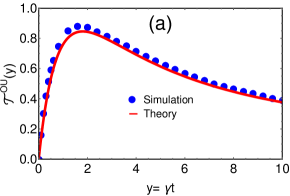
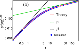
Refer to caption
Refer to caption
Figure 9: (a) Comparision of the scaling function 𝒯O​U​(y)superscriptπ’―π‘‚π‘ˆπ‘¦\mathcal{T}^{OU}(y) obtained in Eq. (107) for AOUPs with the results of numerical simulation. (b) Plot of the asymptotic forms of ⟨xΞ±2​(t)⟩cA​O​U​Psuperscriptsubscriptdelimited-⟨⟩superscriptsubscriptπ‘₯𝛼2π‘‘π‘π΄π‘‚π‘ˆπ‘ƒ\langle x_{\alpha}^{2}(t)\rangle_{c}^{AOUP} obtained in Eqs. (110) for Ο„kβ‰ͺtβ‰ͺΟ„Amuch-less-thansubscriptπœπ‘˜π‘‘much-less-thansubscript𝜏𝐴\tau_{k}\ll t\ll\tau_{A} (shown by black dotted line) and Ο„kβ‰ͺΟ„Aβ‰ͺtmuch-less-thansubscriptπœπ‘˜subscript𝜏𝐴much-less-than𝑑\tau_{k}\ll\tau_{A}\ll t (shown by green dotted line) where Ο„A=1Ξ³subscript𝜏𝐴1𝛾\tau_{A}=\frac{1}{\gamma}. The pink solid line corresponds to the theoretical result in Eq. (106) while the blue filled circles correspond to the numerical simulation. For both plots, we have chosen K=2,Ξ³=0.5formulae-sequence𝐾2𝛾0.5K=2,~{}\gamma=0.5 and D=0.2𝐷0.2D=0.2. The simulation is done with N=100𝑁100N=100 particles on a ring.

4 MSD, COVARIANCE AND TWO POINT CORRELATION FOR AOUP CHAIN

In this section, we investigate the correlations in the positions of the tagged particles for the AOUP chain. To this end, we use the correlation ⟨FΒ―sA​O​U​P​(Ο„1)​FΒ―sA​O​U​Pβ£βˆ—β€‹(Ο„2)⟩csubscriptdelimited-⟨⟩superscriptsubscriptΒ―πΉπ‘ π΄π‘‚π‘ˆπ‘ƒsubscript𝜏1superscriptsubscriptΒ―πΉπ‘ π΄π‘‚π‘ˆπ‘ƒsubscript𝜏2𝑐\langle\bar{F}_{s}^{AOUP}(\tau_{1})\bar{F}_{s}^{AOUP*}(\tau_{2})\rangle_{c} in Eq. (170) to write the unequal time correlation for the Fourier variables xΒ―s​(t)subscriptΒ―π‘₯𝑠𝑑\bar{x}_{s}(t) as

⟨xΒ―s​(t1)​xΒ―sβ€²βˆ—β€‹(t2)⟩cA​O​U​P=Ξ΄s,s′​Dγ​N​ℋ1​(Ξ³,as,t1,t2),subscriptsuperscriptdelimited-⟨⟩subscriptΒ―π‘₯𝑠subscript𝑑1superscriptsubscriptΒ―π‘₯superscript𝑠′subscript𝑑2π΄π‘‚π‘ˆπ‘ƒπ‘subscript𝛿𝑠superscript𝑠′𝐷𝛾𝑁subscriptβ„‹1𝛾subscriptπ‘Žπ‘ subscript𝑑1subscript𝑑2\displaystyle\langle\bar{x}_{s}(t_{1})\bar{x}_{s^{\prime}}^{*}(t_{2})\rangle^{AOUP}_{c}=\delta_{s,s^{\prime}}\frac{D}{\gamma N}~{}\mathcal{H}_{1}\left(\gamma,a_{s},t_{1},t_{2}\right), (99)

where assubscriptπ‘Žπ‘ a_{s} is in Eq. (26) and β„‹1​(a,b,t1,t2)subscriptβ„‹1π‘Žπ‘subscript𝑑1subscript𝑑2\mathcal{H}_{1}(a,b,t_{1},t_{2}) is given by

β„‹1​(a,b,t1,t2)=ℋ​(a,b,t1,t2)βˆ’(eβˆ’b​t1βˆ’eβˆ’a​t1)​(eβˆ’b​t2βˆ’eβˆ’a​t2)(bβˆ’a)2subscriptβ„‹1π‘Žπ‘subscript𝑑1subscript𝑑2β„‹π‘Žπ‘subscript𝑑1subscript𝑑2superscript𝑒𝑏subscript𝑑1superscriptπ‘’π‘Žsubscript𝑑1superscript𝑒𝑏subscript𝑑2superscriptπ‘’π‘Žsubscript𝑑2superscriptπ‘π‘Ž2\displaystyle\mathcal{H}_{1}(a,b,t_{1},t_{2})=\mathcal{H}(a,b,t_{1},t_{2})-\frac{\left(e^{-bt_{1}}-e^{-at_{1}}\right)\left(e^{-bt_{2}}-e^{-at_{2}}\right)}{(b-a)^{2}} (100)

with ℋ​(a,b,t1,t2)β„‹π‘Žπ‘subscript𝑑1subscript𝑑2\mathcal{H}(a,b,t_{1},t_{2}) given in Eq. (55). Here also, we take t1≀t2subscript𝑑1subscript𝑑2t_{1}\leq t_{2} without loss of generality. Proceeding further, we use ⟨xΒ―s​(t1)​xΒ―sβ€²βˆ—β€‹(t2)⟩cA​O​U​Psubscriptsuperscriptdelimited-⟨⟩subscriptΒ―π‘₯𝑠subscript𝑑1superscriptsubscriptΒ―π‘₯superscript𝑠′subscript𝑑2π΄π‘‚π‘ˆπ‘ƒπ‘\langle\bar{x}_{s}(t_{1})\bar{x}_{s^{\prime}}^{*}(t_{2})\rangle^{AOUP}_{c} in Eq. (99) to write the unequal time correlation as

⟨x0​(t1)​xβ​(t2)⟩cA​O​U​Psuperscriptsubscriptdelimited-⟨⟩subscriptπ‘₯0subscript𝑑1subscriptπ‘₯𝛽subscript𝑑2π‘π΄π‘‚π‘ˆπ‘ƒ\displaystyle\langle x_{0}(t_{1})x_{\beta}(t_{2})\rangle_{c}^{AOUP} =βˆ‘s,sβ€²=0Nβˆ’1eβˆ’2​i​π​β​sNβ€‹βŸ¨xΒ―s​(t1)​xΒ―s′​(t2)⟩cA​O​U​P,absentsuperscriptsubscript𝑠superscript𝑠′0𝑁1superscript𝑒2π‘–πœ‹π›½π‘ π‘superscriptsubscriptdelimited-⟨⟩subscriptΒ―π‘₯𝑠subscript𝑑1subscriptΒ―π‘₯superscript𝑠′subscript𝑑2π‘π΄π‘‚π‘ˆπ‘ƒ\displaystyle=\sum_{s,s^{\prime}=0}^{N-1}e^{-\frac{2i\pi\beta s}{N}}\langle\bar{x}_{s}(t_{1})\bar{x}_{s^{\prime}}(t_{2})\rangle_{c}^{AOUP}, (101)
=Dγ​Nβ€‹βˆ‘s=0Nβˆ’1cos⁑(2​π​s​βN)​ℋ1​(Ξ³,as,t1,t2).absent𝐷𝛾𝑁superscriptsubscript𝑠0𝑁12πœ‹π‘ π›½π‘subscriptβ„‹1𝛾subscriptπ‘Žπ‘ subscript𝑑1subscript𝑑2\displaystyle=\frac{D}{\gamma N}\sum_{s=0}^{N-1}\cos\left(\frac{2\pi s\beta}{N}\right)\mathcal{H}_{1}\left(\gamma,a_{s},t_{1},t_{2}\right). (102)

In going to the second line, we substitute ⟨xΒ―s​(t1)​xΒ―s′​(t2)⟩cA​O​U​Psuperscriptsubscriptdelimited-⟨⟩subscriptΒ―π‘₯𝑠subscript𝑑1subscriptΒ―π‘₯superscript𝑠′subscript𝑑2π‘π΄π‘‚π‘ˆπ‘ƒ\langle\bar{x}_{s}(t_{1})\bar{x}_{s^{\prime}}(t_{2})\rangle_{c}^{AOUP} from Eq. (99). Note that for Ξ²=0𝛽0\beta=0 and t1=t2subscript𝑑1subscript𝑑2t_{1}=t_{2}, Eq. (102) reduces to the MSD of the tagged particle. On the other hand, for Ξ²β‰ 0𝛽0\beta\neq 0 and t1=t2subscript𝑑1subscript𝑑2t_{1}=t_{2}, it reduces to the covariance of the positions of the tagged particles. Similarly, for Ξ²=0𝛽0\beta=0 and t1β‰ t2subscript𝑑1subscript𝑑2t_{1}\neq t_{2}, Eq. (102) becomes the position auto correlation. In what follows, we look at ⟨x0​(t1)​xβ​(t2)⟩cA​O​U​Psuperscriptsubscriptdelimited-⟨⟩subscriptπ‘₯0subscript𝑑1subscriptπ‘₯𝛽subscript𝑑2π‘π΄π‘‚π‘ˆπ‘ƒ\langle x_{0}(t_{1})x_{\beta}(t_{2})\rangle_{c}^{AOUP} and use it to study the MSD, covariance and position auto correlation by suitably changing Ξ²,t1𝛽subscript𝑑1\beta,~{}t_{1} and t2subscript𝑑2t_{2}.

As seen for RTP, the correlation function ⟨x0​(t1)​xβ​(t2)⟩cA​O​U​Psuperscriptsubscriptdelimited-⟨⟩subscriptπ‘₯0subscript𝑑1subscriptπ‘₯𝛽subscript𝑑2π‘π΄π‘‚π‘ˆπ‘ƒ\langle x_{0}(t_{1})x_{\beta}(t_{2})\rangle_{c}^{AOUP} possesses various interesting scaling behaviours depending on where the observation time t𝑑t lies. To decipher these scaling forms, we analyse Eq. (102) in the limit Nβ†’βˆžβ†’π‘N\to\infty for which we change the summation in the R.H.S. to the integration and rewrite

⟨x0​(t1)​xβ​(t2)⟩cA​O​U​P≃D2β€‹Ο€β€‹Ξ³β€‹βˆ«βˆ’Ο€Ο€π‘‘q​cos⁑(q​β)​ℋ1​(Ξ³,bq,t1,t2),similar-to-or-equalssuperscriptsubscriptdelimited-⟨⟩subscriptπ‘₯0subscript𝑑1subscriptπ‘₯𝛽subscript𝑑2π‘π΄π‘‚π‘ˆπ‘ƒπ·2πœ‹π›Ύsuperscriptsubscriptπœ‹πœ‹differential-dπ‘žπ‘žπ›½subscriptβ„‹1𝛾subscriptπ‘π‘žsubscript𝑑1subscript𝑑2\displaystyle\langle x_{0}(t_{1})x_{\beta}(t_{2})\rangle_{c}^{AOUP}\simeq\frac{D}{2\pi\gamma}\int_{-\pi}^{\pi}dq\cos\left(q\beta\right)~{}\mathcal{H}_{1}\left(\gamma,b_{q},t_{1},t_{2}\right), (103)

where bq=4​K​sin2⁑(q/2)subscriptπ‘π‘ž4𝐾superscript2π‘ž2b_{q}=4K\sin^{2}\left(q/2\right). In conjunction with the previous case of RTP, we analyse this expression for (i) t1β‰ͺΟ„k,t2β‰ͺΟ„Kformulae-sequencemuch-less-thansubscript𝑑1subscriptπœπ‘˜much-less-thansubscript𝑑2subscript𝜏𝐾t_{1}\ll\tau_{k},~{}t_{2}\ll\tau_{K} and (ii) t1≫τK,t2≫τKformulae-sequencemuch-greater-thansubscript𝑑1subscript𝜏𝐾much-greater-thansubscript𝑑2subscript𝜏𝐾t_{1}\gg\tau_{K},~{}t_{2}\gg\tau_{K} keeping t2t1subscript𝑑2subscript𝑑1\frac{t_{2}}{t_{1}} fixed.

Refer to caption
Refer to caption
Figure 10: (a) Illustration of the scaling function 𝒫O​U​(y,tr)superscriptπ’«π‘‚π‘ˆπ‘¦subscriptπ‘‘π‘Ÿ\mathcal{P}^{OU}(y,t_{r}) in Eq. (112) associated with ⟨x0​(t1)​xβ​(t2)⟩cA​O​U​Psuperscriptsubscriptdelimited-⟨⟩subscriptπ‘₯0subscript𝑑1subscriptπ‘₯𝛽subscript𝑑2π‘π΄π‘‚π‘ˆπ‘ƒ\langle x_{0}(t_{1})x_{\beta}(t_{2})\rangle_{c}^{AOUP}. We have shown comparision with the results of numerical simulation obtained for three sets of t1subscript𝑑1t_{1} and t2subscript𝑑2t_{2} keeping the ratio tr=t2t1subscriptπ‘‘π‘Ÿsubscript𝑑2subscript𝑑1t_{r}=\frac{t_{2}}{t_{1}} fixed which for our case is tr=2subscriptπ‘‘π‘Ÿ2t_{r}=2. We have chosen D=0.2𝐷0.2D=0.2, K=2𝐾2K=2, Ξ³=0.001𝛾0.001\gamma=0.001 and N=100𝑁100N=100. (b) Comparision of 𝒬​(y,tr)𝒬𝑦subscriptπ‘‘π‘Ÿ\mathcal{Q}(y,t_{r}) in Eq. (117) with the same obtained from the simulation of AOUP dynamics. The comparision is shown for three sets of t1subscript𝑑1t_{1} and t2subscript𝑑2t_{2} with tr=t2t1subscriptπ‘‘π‘Ÿsubscript𝑑2subscript𝑑1t_{r}=\frac{t_{2}}{t_{1}} fixed which again is chosen as tr=2subscriptπ‘‘π‘Ÿ2t_{r}=2. The parameters taken are D=0.2𝐷0.2D=0.2, K=2𝐾2K=2, Ξ³=1𝛾1\gamma=1 and N=200𝑁200N=200.

4.1 Case I: t1β‰ͺΟ„K,t2β‰ͺΟ„Kformulae-sequencemuch-less-thansubscript𝑑1subscript𝜏𝐾much-less-thansubscript𝑑2subscript𝜏𝐾t_{1}\ll\tau_{K},~{}t_{2}\ll\tau_{K}:

Let us consider ⟨x0​(t1)​xβ​(t2)⟩cA​O​U​Psuperscriptsubscriptdelimited-⟨⟩subscriptπ‘₯0subscript𝑑1subscriptπ‘₯𝛽subscript𝑑2π‘π΄π‘‚π‘ˆπ‘ƒ\langle x_{0}(t_{1})x_{\beta}(t_{2})\rangle_{c}^{AOUP} when t1β‰ͺΟ„Kmuch-less-thansubscript𝑑1subscript𝜏𝐾t_{1}\ll\tau_{K}, t2β‰ͺΟ„Kmuch-less-thansubscript𝑑2subscript𝜏𝐾t_{2}\ll\tau_{K} while the ratio t2t1subscript𝑑2subscript𝑑1\frac{t_{2}}{t_{1}} is kept fixed. Since Ο„Ksubscript𝜏𝐾\tau_{K} is the smallest time scale, t1subscript𝑑1t_{1} and t2subscript𝑑2t_{2} are smaller than all the time scales present in the model. Therefore we expand the R.H.S. of Eq. (103) in t1subscript𝑑1t_{1} and t2subscript𝑑2t_{2}. By direct expansion of Eq. (100), we find that β„‹1​(m,n,t1,t2)≃m​t12​(t2βˆ’t13)similar-to-or-equalssubscriptβ„‹1π‘šπ‘›subscript𝑑1subscript𝑑2π‘šsuperscriptsubscript𝑑12subscript𝑑2subscript𝑑13\mathcal{H}_{1}(m,n,t_{1},t_{2})\simeq mt_{1}^{2}\left(t_{2}-\frac{t_{1}}{3}\right) inserting which in Eq. (103), we find

⟨x0​(t1)​xβ​(t2)⟩cA​O​U​P≃D​t12​(t2βˆ’t13)​δβ,0,as ​t1≀t2β‰ͺΟ„K.formulae-sequencesimilar-to-or-equalssuperscriptsubscriptdelimited-⟨⟩subscriptπ‘₯0subscript𝑑1subscriptπ‘₯𝛽subscript𝑑2π‘π΄π‘‚π‘ˆπ‘ƒπ·superscriptsubscript𝑑12subscript𝑑2subscript𝑑13subscript𝛿𝛽0asΒ subscript𝑑1subscript𝑑2much-less-thansubscript𝜏𝐾\displaystyle\langle x_{0}(t_{1})x_{\beta}(t_{2})\rangle_{c}^{AOUP}\simeq Dt_{1}^{2}\left(t_{2}-\frac{t_{1}}{3}\right)\delta_{\beta,0},~{}~{}~{}~{}~{}~{}\text{as }t_{1}\leq t_{2}\ll\tau_{K}. (104)

Since the particles do not feel the presence of other particles when t1β‰ͺΟ„Kmuch-less-thansubscript𝑑1subscript𝜏𝐾t_{1}\ll\tau_{K} and t2β‰ͺΟ„Kmuch-less-thansubscript𝑑2subscript𝜏𝐾t_{2}\ll\tau_{K}, we get zero correlation for Ξ²β‰ 0𝛽0\beta\neq 0. Also, for Ξ²=0𝛽0\beta=0 and t1=t2=tsubscript𝑑1subscript𝑑2𝑑t_{1}=t_{2}=t, we find ⟨x02​(t)⟩cA​O​U​P≃2​D3​t3similar-to-or-equalssuperscriptsubscriptdelimited-⟨⟩superscriptsubscriptπ‘₯02π‘‘π‘π΄π‘‚π‘ˆπ‘ƒ2𝐷3superscript𝑑3\langle x_{0}^{2}(t)\rangle_{c}^{AOUP}\simeq\frac{2D}{3}t^{3} which is just the MSD for a single AOUP.

4.2 Case II: t1≫τK,t2≫τKformulae-sequencemuch-greater-thansubscript𝑑1subscript𝜏𝐾much-greater-thansubscript𝑑2subscript𝜏𝐾t_{1}\gg\tau_{K},~{}t_{2}\gg\tau_{K}:

We next look at ⟨x0​(t1)​xβ​(t2)⟩cA​O​U​Psuperscriptsubscriptdelimited-⟨⟩subscriptπ‘₯0subscript𝑑1subscriptπ‘₯𝛽subscript𝑑2π‘π΄π‘‚π‘ˆπ‘ƒ\langle x_{0}(t_{1})x_{\beta}(t_{2})\rangle_{c}^{AOUP} in Eq. (103) in the limit when t1≫τKmuch-greater-thansubscript𝑑1subscript𝜏𝐾t_{1}\gg\tau_{K} and t2≫τKmuch-greater-thansubscript𝑑2subscript𝜏𝐾t_{2}\gg\tau_{K} keeping t2/t1subscript𝑑2subscript𝑑1t_{2}/t_{1} fixed. Proceeding as for the RTP chain (see discussion above Eq. (75)), it is easy to show that Eq. (103) yields

⟨x0​(t1)​xβ​(t2)⟩cA​O​U​P≃similar-to-or-equalssuperscriptsubscriptdelimited-⟨⟩subscriptπ‘₯0subscript𝑑1subscriptπ‘₯𝛽subscript𝑑2π‘π΄π‘‚π‘ˆπ‘ƒabsent\displaystyle\langle x_{0}(t_{1})x_{\beta}(t_{2})\rangle_{c}^{AOUP}\simeq D2​π​γ​t13Kβ€‹βˆ«βˆ’βˆžβˆžπ‘‘w​cos⁑(w​βK​t1)​ℋ1​(γ​t1,w2,1,t2t1).𝐷2πœ‹π›Ύsuperscriptsubscript𝑑13𝐾superscriptsubscriptdifferential-d𝑀𝑀𝛽𝐾subscript𝑑1subscriptβ„‹1𝛾subscript𝑑1superscript𝑀21subscript𝑑2subscript𝑑1\displaystyle\frac{D}{2\pi\gamma}\sqrt{\frac{t_{1}^{3}}{K}}\int_{-\infty}^{\infty}dw\cos\left(\frac{w\beta}{\sqrt{Kt_{1}}}\right)\mathcal{H}_{1}\left(\gamma t_{1},w^{2},1,\frac{t_{2}}{t_{1}}\right). (105)

4.2.1 MSD:

We first look at the MSD ⟨x02​(t)⟩cA​B​Psuperscriptsubscriptdelimited-⟨⟩superscriptsubscriptπ‘₯02𝑑𝑐𝐴𝐡𝑃\langle x_{0}^{2}(t)\rangle_{c}^{ABP} which is otained by putting Ξ²=0𝛽0\beta=0 and t1=t2=tsubscript𝑑1subscript𝑑2𝑑t_{1}=t_{2}=t in Eq. (105). Inserting these values, we find that the MSD possesses the scaling form

⟨x02​(t)⟩cA​O​U​Psuperscriptsubscriptdelimited-⟨⟩superscriptsubscriptπ‘₯02π‘‘π‘π΄π‘‚π‘ˆπ‘ƒ\displaystyle\langle x_{0}^{2}(t)\rangle_{c}^{AOUP} ≃D​t322​π​γ​K​𝒯O​U​(γ​t),for ​t≫τK,formulae-sequencesimilar-to-or-equalsabsent𝐷superscript𝑑322πœ‹π›ΎπΎsuperscriptπ’―π‘‚π‘ˆπ›Ύπ‘‘much-greater-thanfor 𝑑subscript𝜏𝐾\displaystyle\simeq\frac{Dt^{\frac{3}{2}}}{2\pi\gamma\sqrt{K}}~{}\mathcal{T}^{OU}\left(\gamma t\right),~{}~{}~{}~{}~{}~{}~{}~{}\text{for }t\gg\tau_{K}, (106)

where the scaling function 𝒯O​U​(y)superscriptπ’―π‘‚π‘ˆπ‘¦\mathcal{T}^{OU}(y) is given by

𝒯O​U​(y)=βˆ«βˆ’βˆžβˆžπ‘‘w​ℋ1​(y,w2,1,1).superscriptπ’―π‘‚π‘ˆπ‘¦superscriptsubscriptdifferential-d𝑀subscriptβ„‹1𝑦superscript𝑀211\displaystyle\mathcal{T}^{OU}(y)=\int_{-\infty}^{\infty}~{}dw~{}\mathcal{H}_{1}\left(y,w^{2},1,1\right). (107)

In Figure 9(a), we have plotted 𝒯O​U​(y)superscriptπ’―π‘‚π‘ˆπ‘¦\mathcal{T}^{OU}(y) and compared against the same obtained from numerical simulation. We observe an excellent agreement. Proceeding further, we analyse the asymptotic forms of 𝒯O​U​(y)superscriptπ’―π‘‚π‘ˆπ‘¦\mathcal{T}^{OU}(y) for yβ†’0→𝑦0y\to 0 and yβ†’βˆžβ†’π‘¦y\to\infty. To get the these forms, we expand the term inside integral on the R.H.S. of Eq. (107) in these limits. It is straightforward to show that the asymptotic forms read

𝒯O​U​(y)superscriptπ’―π‘‚π‘ˆπ‘¦\displaystyle\mathcal{T}^{OU}(y) ≃32​π15​(2βˆ’1)​yβˆ’32​π105​(8​2βˆ’9)​y2,as ​yβ†’0,formulae-sequencesimilar-to-or-equalsabsent32πœ‹1521𝑦32πœ‹105829superscript𝑦2β†’as 𝑦0\displaystyle\simeq\frac{32\sqrt{\pi}}{15}\left(\sqrt{2}-1\right)y-{\frac{32\sqrt{\pi}}{105}\left(8\sqrt{2}-9\right)y^{2}},~{}~{}~{}~{}~{}\text{as }y\to 0,
≃2​2​πy+O​(yβˆ’2),as ​yβ†’βˆž.formulae-sequencesimilar-to-or-equalsabsent22πœ‹π‘¦π‘‚superscript𝑦2β†’as 𝑦\displaystyle\simeq\frac{2\sqrt{2\pi}}{y}+O(y^{-2}),~{}~{}~{}~{}~{}~{}~{}~{}~{}~{}~{}~{}~{}~{}~{}~{}~{}~{}~{}~{}~{}~{}~{}~{}~{}~{}~{}~{}~{}~{}~{}~{}~{}~{}~{}~{}~{}~{}\text{as }y\to\infty. (108)

Using these asymptotic forms, we find that there is crossover from t52superscript𝑑52t^{\frac{5}{2}} to t𝑑\sqrt{t} at t∼1Ξ³similar-to𝑑1𝛾t\sim\frac{1}{\gamma} as

⟨x02​(t)⟩cA​O​U​Psuperscriptsubscriptdelimited-⟨⟩superscriptsubscriptπ‘₯02π‘‘π‘π΄π‘‚π‘ˆπ‘ƒ\displaystyle\langle x_{0}^{2}(t)\rangle_{c}^{AOUP} ≃16​(2βˆ’1)​D15​π​K​t52+O​(t72),for ​tβ‰ͺ1Ξ³,formulae-sequencesimilar-to-or-equalsabsent1621𝐷15πœ‹πΎsuperscript𝑑52𝑂superscript𝑑72much-less-thanfor 𝑑1𝛾\displaystyle\simeq\frac{16(\sqrt{2}-1)D}{15\sqrt{\pi K}}t^{\frac{5}{2}}+O\left(t^{\frac{7}{2}}\right),~{}~{}~{}~{}~{}~{}~{}~{}~{}~{}\text{for }t\ll\frac{1}{\gamma}, (109)
≃DΞ³2​2​tπ​K+O​(tβˆ’12),for ​t≫1Ξ³.formulae-sequencesimilar-to-or-equalsabsent𝐷superscript𝛾22π‘‘πœ‹πΎπ‘‚superscript𝑑12much-greater-thanfor 𝑑1𝛾\displaystyle\simeq\frac{D}{\gamma^{2}}\sqrt{\frac{2t}{\pi K}}+O\left(t^{-\frac{1}{2}}\right),~{}~{}~{}~{}~{}~{}~{}~{}~{}~{}~{}~{}~{}~{}~{}~{}~{}\text{for }t\gg\frac{1}{\gamma}. (110)

Quite remarkably for tβ‰ͺΟ„Amuch-less-than𝑑subscript𝜏𝐴t\ll\tau_{A}, we find that the MSD scales as ∼t52similar-toabsentsuperscript𝑑52\sim t^{\frac{5}{2}} for AOUP which is different than ∼t32similar-toabsentsuperscript𝑑32\sim t^{\frac{3}{2}} scaling for RTP as seen in Eq. (40). Again, this scaling arises due to the interplay of the activity and interactions between the particles. The caging effect due to the interactions causes the scaling of the MSD to change from t3superscript𝑑3t^{3} to t52superscript𝑑52t^{\frac{5}{2}}. On the other hand, for t≫τAmuch-greater-than𝑑subscript𝜏𝐴t\gg\tau_{A}, both models give ∼tsimilar-toabsent𝑑\sim\sqrt{t} scaling for the MSD. In Figure 9(b), we have illustrated this cross-over behaviour from t5/2superscript𝑑52t^{5/2} to t1/2superscript𝑑12t^{1/2} by comparing them against the same obtained from numerical simulation. As seen in Figure 9(b), the asymptotic results of Eqs. (109) and (110) are consistent with the numerical simulation. Finally, we allude that a similar scaling form as in Eq. (107) was conjectured in [75] for the AOUPs with hadrcore interaction even though exact form of the scaling function was not obtained. Our consideration of the simple model of harmonic chain has given both the scaling form and the scaling function.

Coming back to ⟨x0​(t1)​xβ​(t2)⟩cA​O​U​Psuperscriptsubscriptdelimited-⟨⟩subscriptπ‘₯0subscript𝑑1subscriptπ‘₯𝛽subscript𝑑2π‘π΄π‘‚π‘ˆπ‘ƒ\langle x_{0}(t_{1})x_{\beta}(t_{2})\rangle_{c}^{AOUP} in Eq. (105), we study this expression in various limits of γ​t1𝛾subscript𝑑1\gamma t_{1} to get the effect of activity in the correlation function. In what follows, we look at ⟨x0​(t1)​xβ​(t2)⟩cA​O​U​Psuperscriptsubscriptdelimited-⟨⟩subscriptπ‘₯0subscript𝑑1subscriptπ‘₯𝛽subscript𝑑2π‘π΄π‘‚π‘ˆπ‘ƒ\langle x_{0}(t_{1})x_{\beta}(t_{2})\rangle_{c}^{AOUP} for t1≀t2β‰ͺΟ„Asubscript𝑑1subscript𝑑2much-less-thansubscript𝜏𝐴t_{1}\leq t_{2}\ll\tau_{A} and Ο„Aβ‰ͺt1≀t2much-less-thansubscript𝜏𝐴subscript𝑑1subscript𝑑2\tau_{A}\ll t_{1}\leq t_{2} separately.

Refer to caption
Refer to caption
Figure 11: Comparision of the scaling forms obtained for ⟨xα​(t1)​xα​(t2)⟩cA​O​U​Psuperscriptsubscriptdelimited-⟨⟩subscriptπ‘₯𝛼subscript𝑑1subscriptπ‘₯𝛼subscript𝑑2π‘π΄π‘‚π‘ˆπ‘ƒ\langle x_{\alpha}(t_{1})x_{\alpha}(t_{2})\rangle_{c}^{AOUP} in Eqs. (114) and (118) for tβ‰ͺ1Ξ³much-less-than𝑑1𝛾t\ll\frac{1}{\gamma} and t≫1Ξ³much-greater-than𝑑1𝛾t\gg\frac{1}{\gamma} respectively. In both (a) and (b), the black solid line is the analytical results in in Eqs. (114) and (118) respectively, while the symbols correspond to the simulation data for different values of t1subscript𝑑1t_{1}. We have taken Ξ³=0.001𝛾0.001\gamma=0.001 for plot (a) and Ξ³=2𝛾2\gamma=2 for plot (b). For both plots, simulation is done for N=100𝑁100N=100 particles with K=3𝐾3K=3 and D=0.2𝐷0.2D=0.2.

4.2.2 Covariance and unequal time correlations for t1β‰ͺΟ„A,t2β‰ͺΟ„Aformulae-sequencemuch-less-thansubscript𝑑1subscript𝜏𝐴much-less-thansubscript𝑑2subscript𝜏𝐴{t_{1}\ll\tau_{A},~{}t_{2}\ll\tau_{A}}:

Let us first look at ⟨x0​(t1)​xβ​(t2)⟩cA​O​U​Psuperscriptsubscriptdelimited-⟨⟩subscriptπ‘₯0subscript𝑑1subscriptπ‘₯𝛽subscript𝑑2π‘π΄π‘‚π‘ˆπ‘ƒ\langle x_{0}(t_{1})x_{\beta}(t_{2})\rangle_{c}^{AOUP} in Eq. (105) when both t1subscript𝑑1t_{1} and t2subscript𝑑2t_{2} are smaller than the activity time scale Ο„A=1Ξ³subscript𝜏𝐴1𝛾\tau_{A}=\frac{1}{\gamma}. For γ​t1β†’0→𝛾subscript𝑑10\gamma t_{1}\to 0, we can expand β„‹1​(γ​t1,w2,1,tr)subscriptβ„‹1𝛾subscript𝑑1superscript𝑀21subscriptπ‘‘π‘Ÿ\mathcal{H}_{1}(\gamma t_{1},w^{2},1,t_{r}) in Eq. (105) in γ​t1𝛾subscript𝑑1\gamma t_{1} which gives β„‹1​(γ​t1,w2,1,tr)≃γ​t1w6​[βˆ’2+2​eβˆ’w2βˆ’eβˆ’(tr+1)​w2+2​eβˆ’tr​w2βˆ’eβˆ’(trβˆ’1)​w2+2​w2]similar-to-or-equalssubscriptβ„‹1𝛾subscript𝑑1superscript𝑀21subscriptπ‘‘π‘Ÿπ›Ύsubscript𝑑1superscript𝑀6delimited-[]22superscript𝑒superscript𝑀2superscript𝑒subscriptπ‘‘π‘Ÿ1superscript𝑀22superscript𝑒subscriptπ‘‘π‘Ÿsuperscript𝑀2superscript𝑒subscriptπ‘‘π‘Ÿ1superscript𝑀22superscript𝑀2\mathcal{H}_{1}(\gamma t_{1},w^{2},1,t_{r})\simeq\frac{\gamma t_{1}}{w^{6}}\left[-2+2e^{-w^{2}}-e^{-(t_{r}+1)w^{2}}+2e^{-t_{r}w^{2}}-e^{-(t_{r}-1)w^{2}}+2w^{2}\right] up to leading order in γ​t1𝛾subscript𝑑1\gamma t_{1}. Substituting this expression in Eq. (105) and performing the integration over w𝑀w, we find that ⟨x0​(t1)​xβ​(t2)⟩cA​O​U​Psuperscriptsubscriptdelimited-⟨⟩subscriptπ‘₯0subscript𝑑1subscriptπ‘₯𝛽subscript𝑑2π‘π΄π‘‚π‘ˆπ‘ƒ\langle x_{0}(t_{1})x_{\beta}(t_{2})\rangle_{c}^{AOUP} has the scaling form

⟨x0​(t1)​xβ​(t2)⟩cA​O​U​P≃D2​π​t15K​𝒫O​U​(Ξ²2​K​t1,t2t1),for ​t1≀t2β‰ͺ1Ξ³,formulae-sequencesimilar-to-or-equalssuperscriptsubscriptdelimited-⟨⟩subscriptπ‘₯0subscript𝑑1subscriptπ‘₯𝛽subscript𝑑2π‘π΄π‘‚π‘ˆπ‘ƒπ·2πœ‹superscriptsubscript𝑑15𝐾superscriptπ’«π‘‚π‘ˆπ›½2𝐾subscript𝑑1subscript𝑑2subscript𝑑1forΒ subscript𝑑1subscript𝑑2much-less-than1𝛾\displaystyle\langle x_{0}(t_{1})x_{\beta}(t_{2})\rangle_{c}^{AOUP}\simeq\frac{D}{2\pi}\sqrt{\frac{t_{1}^{5}}{K}}~{}\mathcal{P}^{OU}\left(\frac{\beta}{\sqrt{2Kt_{1}}},\frac{t_{2}}{t_{1}}\right),~{}~{}~{}~{}~{}~{}~{}\text{for }t_{1}\leq t_{2}\ll\frac{1}{\gamma}, (111)

where the scaling function 𝒫O​U​(y,tr)superscriptπ’«π‘‚π‘ˆπ‘¦subscriptπ‘‘π‘Ÿ\mathcal{P}^{OU}\left(y,t_{r}\right) is given by

𝒫O​Usuperscriptπ’«π‘‚π‘ˆ\displaystyle\mathcal{P}^{OU} (y,tr)=Ο€30[21+tr(8+8tr2+9y2+y4+tr(16+9y2))eβˆ’y22​(tr+1)βˆ’302​πyErf(y2)\displaystyle\left(y,\right.\left.t_{r}\right)=\frac{\sqrt{\pi}}{30}\left[2\sqrt{1+t_{r}}\left(8+8t_{r}^{2}+9y^{2}+y^{4}+t_{r}(16+9y^{2})\right)e^{-\frac{y^{2}}{2(t_{r}+1)}}-30\sqrt{2\pi}y\text{Erf}\left(\frac{y}{\sqrt{2}}\right)\right.
βˆ’2​(trβˆ’1)32​(7​trβˆ’7+y2)​eβˆ’y22​(trβˆ’1)βˆ’4​(8+9​y2+y4)​eβˆ’y22βˆ’4​tr​(8​tr2+9​tr​y2+y4)​eβˆ’y22​tr2superscriptsubscriptπ‘‘π‘Ÿ1327subscriptπ‘‘π‘Ÿ7superscript𝑦2superscript𝑒superscript𝑦22subscriptπ‘‘π‘Ÿ1489superscript𝑦2superscript𝑦4superscript𝑒superscript𝑦224subscriptπ‘‘π‘Ÿ8superscriptsubscriptπ‘‘π‘Ÿ29subscriptπ‘‘π‘Ÿsuperscript𝑦2superscript𝑦4superscript𝑒superscript𝑦22subscriptπ‘‘π‘Ÿ\displaystyle-2(t_{r}-1)^{\frac{3}{2}}\left(7t_{r}-7+y^{2}\right)e^{-\frac{y^{2}}{2(t_{r}-1)}}-4\left(8+9y^{2}+y^{4}\right)e^{-\frac{y^{2}}{2}}-4\sqrt{t_{r}}\left(8t_{r}^{2}+9t_{r}y^{2}+y^{4}\right)e^{-\frac{y^{2}}{2t_{r}}}
+(15+15​tr2βˆ’10​y2+y4+10​tr​(βˆ’3+y2))​{2​trβˆ’1​eβˆ’y22​(trβˆ’1)+2​π​y​Erf​(y2​(trβˆ’1))}1515superscriptsubscriptπ‘‘π‘Ÿ210superscript𝑦2superscript𝑦410subscriptπ‘‘π‘Ÿ3superscript𝑦22subscriptπ‘‘π‘Ÿ1superscript𝑒superscript𝑦22subscriptπ‘‘π‘Ÿ12πœ‹π‘¦Erf𝑦2subscriptπ‘‘π‘Ÿ1\displaystyle\left.+\left(15+15t_{r}^{2}-10y^{2}+y^{4}+10t_{r}(-3+y^{2})\right)\Bigg{\{}2\sqrt{t_{r}-1}e^{-\frac{y^{2}}{2(t_{r}-1)}}+\sqrt{2\pi}y\text{Erf}\left(\frac{y}{\sqrt{2(t_{r}-1)}}\right)\Bigg{\}}\right.
+2​2​π​y3​(10+y2)​Erfc​(y2)βˆ’2​2​π​y​(15​tr2+10​tr​y2+y4)​Erf​(y2​tr)22πœ‹superscript𝑦310superscript𝑦2Erfc𝑦222πœ‹π‘¦15superscriptsubscriptπ‘‘π‘Ÿ210subscriptπ‘‘π‘Ÿsuperscript𝑦2superscript𝑦4Erf𝑦2subscriptπ‘‘π‘Ÿ\displaystyle+2\sqrt{2\pi}y^{3}\left(10+y^{2}\right)\text{Erfc}\left(\frac{y}{\sqrt{2}}\right)-2\sqrt{2\pi}y\left(15t_{r}^{2}+10t_{r}y^{2}+y^{4}\right)\text{Erf}\left(\frac{y}{\sqrt{2t_{r}}}\right)
+2​πy(15+15tr2+10y2+y4+10tr(3+y2))Erf(y2​(tr+1))].\displaystyle\left.+\sqrt{2\pi}y\left(15+15t_{r}^{2}+10y^{2}+y^{4}+10t_{r}(3+y^{2})\right)\text{Erf}\left(\frac{y}{\sqrt{2(t_{r}+1)}}\right)\right]. (112)

In Fig. 10(a), we have illustrated the scaling function 𝒫O​U​(y,tr)superscriptπ’«π‘‚π‘ˆπ‘¦subscriptπ‘‘π‘Ÿ\mathcal{P}^{OU}(y,t_{r}) and also compared with the same obtained from numerical simulations. We have conducted the comparision for three sets of t1subscript𝑑1t_{1} and t2subscript𝑑2t_{2} keeping the ratio tr=t2t1subscriptπ‘‘π‘Ÿsubscript𝑑2subscript𝑑1t_{r}=\frac{t_{2}}{t_{1}} constant for all. All simuation data collapse over the analytical result. For large y𝑦y, we find 𝒫O​U​(y,tr)superscriptπ’«π‘‚π‘ˆπ‘¦subscriptπ‘‘π‘Ÿ\mathcal{P}^{OU}(y,t_{r}) decays as ∼yβˆ’6​exp​(βˆ’y22​(tr+1))similar-toabsentsuperscript𝑦6expsuperscript𝑦22subscriptπ‘‘π‘Ÿ1\sim y^{-6}~{}\text{exp}\left(-\frac{y^{2}}{2(t_{r}+1)}\right) inserting which in Eq. (111), it is seen that ⟨x0​(t1)​xβ​(t2)⟩cA​O​U​Psuperscriptsubscriptdelimited-⟨⟩subscriptπ‘₯0subscript𝑑1subscriptπ‘₯𝛽subscript𝑑2π‘π΄π‘‚π‘ˆπ‘ƒ\langle x_{0}(t_{1})x_{\beta}(t_{2})\rangle_{c}^{AOUP} has faster than exponential decay with decay length ld=2​K​(t1+t2)subscript𝑙𝑑2𝐾subscript𝑑1subscript𝑑2l_{d}=2\sqrt{K(t_{1}+t_{2})}. On the other hand, for y=0𝑦0y=0, we find that 𝒫O​U​(y=0,tr)=β„’O​U​(tr)superscriptπ’«π‘‚π‘ˆπ‘¦0subscriptπ‘‘π‘Ÿsuperscriptβ„’π‘‚π‘ˆsubscriptπ‘‘π‘Ÿ\mathcal{P}^{OU}(y=0,t_{r})=\mathcal{L}^{OU}(t_{r}) where β„’O​U​(tr)superscriptβ„’π‘‚π‘ˆsubscriptπ‘‘π‘Ÿ\mathcal{L}^{OU}(t_{r}) is given by

β„’O​U​(tr)=8​π15​[(tr+1)5/2+(trβˆ’1)5/2βˆ’2​(1+tr5/2)].superscriptβ„’π‘‚π‘ˆsubscriptπ‘‘π‘Ÿ8πœ‹15delimited-[]superscriptsubscriptπ‘‘π‘Ÿ152superscriptsubscriptπ‘‘π‘Ÿ15221superscriptsubscriptπ‘‘π‘Ÿ52\displaystyle\mathcal{L}^{OU}(t_{r})=\frac{8\sqrt{\pi}}{15}\left[(t_{r}+1)^{5/2}+(t_{r}-1)^{5/2}-2(1+t_{r}^{5/2})\right]. (113)

Inserting this expression in ⟨x0​(t1)​xβ​(t2)⟩cA​O​U​Psuperscriptsubscriptdelimited-⟨⟩subscriptπ‘₯0subscript𝑑1subscriptπ‘₯𝛽subscript𝑑2π‘π΄π‘‚π‘ˆπ‘ƒ\langle x_{0}(t_{1})x_{\beta}(t_{2})\rangle_{c}^{AOUP} in Eq. (111) for Ξ²=0𝛽0\beta=0, we find that the position auto fluctuation satisfies the scaling form

⟨x0​(t1)​x0​(t2)⟩cA​O​U​P≃D2​π​t15K​ℒO​U​(t2t1),for ​t1≀t2β‰ͺ1Ξ³.formulae-sequencesimilar-to-or-equalssuperscriptsubscriptdelimited-⟨⟩subscriptπ‘₯0subscript𝑑1subscriptπ‘₯0subscript𝑑2π‘π΄π‘‚π‘ˆπ‘ƒπ·2πœ‹superscriptsubscript𝑑15𝐾superscriptβ„’π‘‚π‘ˆsubscript𝑑2subscript𝑑1forΒ subscript𝑑1subscript𝑑2much-less-than1𝛾\displaystyle\langle x_{0}(t_{1})x_{0}(t_{2})\rangle_{c}^{AOUP}\simeq\frac{D}{2\pi}\sqrt{\frac{t_{1}^{5}}{K}}~{}\mathcal{L}^{OU}\left(\frac{t_{2}}{t_{1}}\right),~{}~{}~{}~{}~{}~{}~{}\text{for }t_{1}\leq t_{2}\ll\frac{1}{\gamma}. (114)

We have presented the comparision of the scaling function β„’O​U​(tr)superscriptβ„’π‘‚π‘ˆsubscriptπ‘‘π‘Ÿ\mathcal{L}^{OU}(t_{r}) with the same obtained from the numerical simulation in Fig.Β 11(a). We have performed the comparision for three different t1subscript𝑑1t_{1} and for each t1subscript𝑑1t_{1}, we vary t2subscript𝑑2t_{2}. All simulation results match with our theoretical result.

We next look at ⟨x0​(t1)​xβ​(t2)⟩cA​O​U​Psuperscriptsubscriptdelimited-⟨⟩subscriptπ‘₯0subscript𝑑1subscriptπ‘₯𝛽subscript𝑑2π‘π΄π‘‚π‘ˆπ‘ƒ\langle x_{0}(t_{1})x_{\beta}(t_{2})\rangle_{c}^{AOUP} in Eq. (111) for general β𝛽\beta but t1=t2=tsubscript𝑑1subscript𝑑2𝑑t_{1}=t_{2}=t for which it reduces to the covariance. As evident from Eq. (111), the covariance satifies the scaling

⟨x0​(t)​xβ​(t)⟩cA​O​U​P≃D​t522​π​K​ΩO​U​(Ξ²2​K​t),for ​tβ‰ͺ1Ξ³,formulae-sequencesimilar-to-or-equalssuperscriptsubscriptdelimited-⟨⟩subscriptπ‘₯0𝑑subscriptπ‘₯π›½π‘‘π‘π΄π‘‚π‘ˆπ‘ƒπ·superscript𝑑522πœ‹πΎsuperscriptΞ©π‘‚π‘ˆπ›½2𝐾𝑑much-less-thanfor 𝑑1𝛾\displaystyle\langle x_{0}(t)x_{\beta}(t)\rangle_{c}^{AOUP}\simeq\frac{D~{}t^{\frac{5}{2}}}{2\pi\sqrt{K}}~{}\Omega^{OU}\left(\frac{\beta}{\sqrt{2Kt}}\right),~{}~{}~{}~{}~{}~{}\text{for }t\ll\frac{1}{\gamma}, (115)

with the scaling function Ξ©O​U​(y)superscriptΞ©π‘‚π‘ˆπ‘¦\Omega^{OU}(y) given by

Ξ©O​U​(y)=𝒫O​U​(y,tr=1),superscriptΞ©π‘‚π‘ˆπ‘¦superscriptπ’«π‘‚π‘ˆπ‘¦subscriptπ‘‘π‘Ÿ1\displaystyle\Omega^{OU}(y)=\mathcal{P}^{OU}\left(y,t_{r}=1\right), (116)

where 𝒫O​U​(y,tr=1)superscriptπ’«π‘‚π‘ˆπ‘¦subscriptπ‘‘π‘Ÿ1\mathcal{P}^{OU}\left(y,t_{r}=1\right) is given in Eq. (112). In Figure 12(a), we have plotted the scaling function Ξ©O​U​(y)superscriptΞ©π‘‚π‘ˆπ‘¦\Omega^{OU}(y) and compared with the results of the numerical simulations for three different times. We observe an excellent agreement of the theoretical result with that of the simulations. Quite expectedly, this scaling function is different than the same obtained for RTP in Eq. (47). To see this more clearly, we look at the large y𝑦y behaviour of Ξ©O​U​(y)superscriptΞ©π‘‚π‘ˆπ‘¦\Omega^{OU}(y). By direct expansion, we find that Ξ©O​U​(y)∼yβˆ’6​eβˆ’y24similar-tosuperscriptΞ©π‘‚π‘ˆπ‘¦superscript𝑦6superscript𝑒superscript𝑦24\Omega^{OU}(y)\sim y^{-6}~{}e^{-\frac{y^{2}}{4}} which is different than the same obtained in Eq. (49) for RTP. Even though both decay as ∼eβˆ’y24similar-toabsentsuperscript𝑒superscript𝑦24\sim e^{-\frac{y^{2}}{4}}, but the corresponding prefactors are very different.
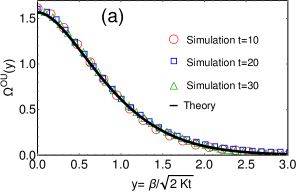
Refer to caption
Refer to caption
Figure 12: (a) Comparision of the scaling function Ξ©O​U​(y)superscriptΞ©π‘‚π‘ˆπ‘¦\Omega^{OU}(y) in Eq. (116) for AOUPs (shown by solid black line) with the results obtained from numerical simulation (shown by symbols) for three different times. We have chosen K=2,Ξ³=0.001formulae-sequence𝐾2𝛾0.001K=2,~{}\gamma=0.001 and D=0.5𝐷0.5D=0.5. (b) Plot of the scaling form and scaling function π’žβ€‹(y)π’žπ‘¦\mathcal{C}(y) obtained in Eqs. (119) and (51) respectively (shown by solid black line) and comparision with the same obtained from numerical simulation for three different values of t𝑑t (shown by different symbols). The parameters chosen are K=2,Ξ³=2formulae-sequence𝐾2𝛾2K=2,~{}\gamma=2 and D=1.7𝐷1.7D=1.7. For both (a) and (b), the simulation is done with N=150𝑁150N=150 particles.

4.2.3 Covariance and unequal time correlations for t1≫τA,t2≫τAformulae-sequencemuch-greater-thansubscript𝑑1subscript𝜏𝐴much-greater-thansubscript𝑑2subscript𝜏𝐴t_{1}\gg\tau_{A},~{}t_{2}\gg\tau_{A}:

We now look at ⟨x0​(t1)​xβ​(t2)⟩cA​O​U​Psuperscriptsubscriptdelimited-⟨⟩subscriptπ‘₯0subscript𝑑1subscriptπ‘₯𝛽subscript𝑑2π‘π΄π‘‚π‘ˆπ‘ƒ\langle x_{0}(t_{1})x_{\beta}(t_{2})\rangle_{c}^{AOUP} in Eq. (105) when both t1subscript𝑑1t_{1} and t2subscript𝑑2t_{2} are larger than the activity time scale Ο„Asubscript𝜏𝐴\tau_{A}. For γ​t1β†’βˆžβ†’π›Ύsubscript𝑑1\gamma t_{1}\to\infty, we use Eq. (100) to approximate β„‹1​(γ​t1,w2,1,tr)≃1γ​t1​w2​(eβˆ’(trβˆ’1)​w2βˆ’eβˆ’(tr+1)​w2)similar-to-or-equalssubscriptβ„‹1𝛾subscript𝑑1superscript𝑀21subscriptπ‘‘π‘Ÿ1𝛾subscript𝑑1superscript𝑀2superscript𝑒subscriptπ‘‘π‘Ÿ1superscript𝑀2superscript𝑒subscriptπ‘‘π‘Ÿ1superscript𝑀2\mathcal{H}_{1}(\gamma t_{1},w^{2},1,t_{r})\simeq\frac{1}{\gamma t_{1}w^{2}}\left(e^{-(t_{r}-1)w^{2}}-e^{-(t_{r}+1)w^{2}}\right) and insert it in Eq. (105) and performing integration over w𝑀w gives the scaling relation

⟨x0​(t1)​xβ​(t2)⟩cA​O​U​P≃DA​2​t1π​K​𝒬​(Ξ²2​K​t1,t2t1),for ​1Ξ³β‰ͺt1≀t2,formulae-sequencesimilar-to-or-equalssuperscriptsubscriptdelimited-⟨⟩subscriptπ‘₯0subscript𝑑1subscriptπ‘₯𝛽subscript𝑑2π‘π΄π‘‚π‘ˆπ‘ƒsubscript𝐷𝐴2subscript𝑑1πœ‹πΎπ’¬π›½2𝐾subscript𝑑1subscript𝑑2subscript𝑑1much-less-thanforΒ 1𝛾subscript𝑑1subscript𝑑2\displaystyle\langle x_{0}(t_{1})x_{\beta}(t_{2})\rangle_{c}^{AOUP}\simeq D_{A}\sqrt{\frac{2t_{1}}{\pi K}}~{}\mathcal{Q}\left(\frac{\beta}{\sqrt{2Kt_{1}}},\frac{t_{2}}{t_{1}}\right),~{}~{}~{}~{}~{}~{}\text{for }\frac{1}{\gamma}\ll t_{1}\leq t_{2}, (117)

where the scaling function 𝒬​(y,tr)𝒬𝑦subscriptπ‘‘π‘Ÿ\mathcal{Q}(y,t_{r}) is given in Eq. (80) and DA=DΞ³2subscript𝐷𝐴𝐷superscript𝛾2D_{A}=\frac{D}{\gamma^{2}}. The result is identical to that of the RTP in Eq. (79) as both models converge to the Brownian motion when t≫τAmuch-greater-than𝑑subscript𝜏𝐴t\gg\tau_{A}. In Fig. 10(b), we have presented a comparision of the scaling function 𝒬​(y,tr)𝒬𝑦subscriptπ‘‘π‘Ÿ\mathcal{Q}(y,t_{r}) with the same obtained from the numerical simulations for three sets t1subscript𝑑1t_{1} and t2subscript𝑑2t_{2}. We observe an excellent match of simulation results with the analytical form of 𝒬​(y,tr)𝒬𝑦subscriptπ‘‘π‘Ÿ\mathcal{Q}(y,t_{r}).

By appropriately manipulating ⟨x0​(t1)​xβ​(t2)⟩cA​O​U​Psuperscriptsubscriptdelimited-⟨⟩subscriptπ‘₯0subscript𝑑1subscriptπ‘₯𝛽subscript𝑑2π‘π΄π‘‚π‘ˆπ‘ƒ\langle x_{0}(t_{1})x_{\beta}(t_{2})\rangle_{c}^{AOUP} in Eq. (117), it is easy to show that the auto correlation and covariance have the scaling form

⟨x0​(t1)​x0​(t2)⟩cA​O​U​P≃DA​2​t1π​K​ℳ​(t2t1),for ​τAβ‰ͺt1≀t2,formulae-sequencesimilar-to-or-equalssuperscriptsubscriptdelimited-⟨⟩subscriptπ‘₯0subscript𝑑1subscriptπ‘₯0subscript𝑑2π‘π΄π‘‚π‘ˆπ‘ƒsubscript𝐷𝐴2subscript𝑑1πœ‹πΎβ„³subscript𝑑2subscript𝑑1much-less-thanforΒ subscript𝜏𝐴subscript𝑑1subscript𝑑2\displaystyle\langle x_{0}(t_{1})x_{0}(t_{2})\rangle_{c}^{AOUP}\simeq D_{A}\sqrt{\frac{2t_{1}}{\pi K}}~{}\mathcal{M}\left(\frac{t_{2}}{t_{1}}\right),~{}~{}~{}~{}~{}~{}~{}~{}~{}~{}~{}~{}\text{for }\tau_{A}\ll t_{1}\leq t_{2}, (118)
⟨x0​(t)​xβ​(t)⟩cA​O​U​P≃DA​2​tπ​Kβ€‹π’žβ€‹(Ξ²2​K​t),for ​t≫τA,formulae-sequencesimilar-to-or-equalssuperscriptsubscriptdelimited-⟨⟩subscriptπ‘₯0𝑑subscriptπ‘₯π›½π‘‘π‘π΄π‘‚π‘ˆπ‘ƒsubscript𝐷𝐴2π‘‘πœ‹πΎπ’žπ›½2𝐾𝑑much-greater-thanfor 𝑑subscript𝜏𝐴\displaystyle\langle x_{0}(t)x_{\beta}(t)\rangle_{c}^{AOUP}\simeq D_{A}\sqrt{\frac{2t}{\pi K}}~{}\mathcal{C}\left(\frac{\beta}{\sqrt{2Kt}}\right),~{}~{}~{}~{}~{}~{}~{}~{}~{}~{}~{}\text{for }t\gg\tau_{A}, (119)

where the scaling functions π’žβ€‹(y)π’žπ‘¦\mathcal{C}(y) and ℳ​(tr)β„³subscriptπ‘‘π‘Ÿ\mathcal{M}(t_{r}) are given in Eqs. (51) and (67) respectively. In Figure 11(b) and 12(b), we have numerically illustrated the scaling relations in Eqs. (118) and (119) respectively. We observe excellent agreement with the numerical simulations. Once again, we emphasise that in this time regime (≫τA)much-greater-thanabsentsubscript𝜏𝐴(\gg\tau_{A}), the scaling functions for RTP and AOUP models are same because they essentially become harmonically coupled chain of Brownian particles.

Before closing this section, we accentuate that for AOUP also, the correlation ⟨x0​(t1)​xβ​(t2)⟩cA​O​U​Psuperscriptsubscriptdelimited-⟨⟩subscriptπ‘₯0subscript𝑑1subscriptπ‘₯𝛽subscript𝑑2π‘π΄π‘‚π‘ˆπ‘ƒ\langle x_{0}(t_{1})x_{\beta}(t_{2})\rangle_{c}^{AOUP} exhibits non-monotonic behaviour with respect to t2subscript𝑑2t_{2}. This is shown in Fig. 6(b) for Ξ²=0𝛽0\beta=0 and Ξ²β‰ 0𝛽0\beta\neq 0 along with the comparision with the simulations. We see that it increases initially with rise in t2subscript𝑑2t_{2}, attains its maximum value and then starts decreasing thereafter. As discussed for RTP, the non-monotonic behaviour can be understood by looking at the asymptotic expressions of ⟨x0​(t1)​xβ​(t2)⟩cA​O​U​Psuperscriptsubscriptdelimited-⟨⟩subscriptπ‘₯0subscript𝑑1subscriptπ‘₯𝛽subscript𝑑2π‘π΄π‘‚π‘ˆπ‘ƒ\langle x_{0}(t_{1})x_{\beta}(t_{2})\rangle_{c}^{AOUP} for t2≫t1much-greater-thansubscript𝑑2subscript𝑑1t_{2}\gg t_{1} when t2β‰ͺ1Ξ³much-less-thansubscript𝑑21𝛾t_{2}\ll\frac{1}{\gamma} and t2≫1Ξ³much-greater-thansubscript𝑑21𝛾t_{2}\gg\frac{1}{\gamma}. When both t1β‰ͺ1Ξ³much-less-thansubscript𝑑11𝛾t_{1}\ll\frac{1}{\gamma} and t2β‰ͺ1Ξ³much-less-thansubscript𝑑21𝛾t_{2}\ll\frac{1}{\gamma}, it can be shown using Eq. (111) that ⟨x0​(t1)​xβ​(t2)⟩cA​O​U​Psuperscriptsubscriptdelimited-⟨⟩subscriptπ‘₯0subscript𝑑1subscriptπ‘₯𝛽subscript𝑑2π‘π΄π‘‚π‘ˆπ‘ƒ\langle x_{0}(t_{1})x_{\beta}(t_{2})\rangle_{c}^{AOUP} increases as ∼t2similar-toabsentsubscript𝑑2\sim\sqrt{t_{2}} for t2≫t1much-greater-thansubscript𝑑2subscript𝑑1t_{2}\gg t_{1}. On the other hand when t1≫τAmuch-greater-thansubscript𝑑1subscript𝜏𝐴t_{1}\gg\tau_{A} and t2≫τAmuch-greater-thansubscript𝑑2subscript𝜏𝐴t_{2}\gg\tau_{A}, using Eq. (117), we find that ⟨x0​(t1)​xβ​(t2)⟩cA​O​U​Psuperscriptsubscriptdelimited-⟨⟩subscriptπ‘₯0subscript𝑑1subscriptπ‘₯𝛽subscript𝑑2π‘π΄π‘‚π‘ˆπ‘ƒ\langle x_{0}(t_{1})x_{\beta}(t_{2})\rangle_{c}^{AOUP} decays as ∼1/t2similar-toabsent1subscript𝑑2\sim 1/\sqrt{t_{2}}. This means that at some intermediate t2subscript𝑑2t_{2}, it will exhibit the maximum value.

4.3 Large but finite N𝑁N:

We now look at the correlation ⟨x0​(t1)​xβ​(t2)⟩cA​O​U​Psuperscriptsubscriptdelimited-⟨⟩subscriptπ‘₯0subscript𝑑1subscriptπ‘₯𝛽subscript𝑑2π‘π΄π‘‚π‘ˆπ‘ƒ\langle x_{0}(t_{1})x_{\beta}(t_{2})\rangle_{c}^{AOUP} when N𝑁N is large but has finite value. As done for RTP, one can, in principle, start from the the exact expression of ⟨x0​(t1)​xβ​(t2)⟩cA​O​U​Psuperscriptsubscriptdelimited-⟨⟩subscriptπ‘₯0subscript𝑑1subscriptπ‘₯𝛽subscript𝑑2π‘π΄π‘‚π‘ˆπ‘ƒ\langle x_{0}(t_{1})x_{\beta}(t_{2})\rangle_{c}^{AOUP} in Eq. (102) and analyse it for the large but finite N𝑁N case. However, we follow a different route by noting that the dynamics of RTP and AOUP are identical to that of the Brownian motion when the obervation time is larger than the activity time scale. Hence the scaling results obtained in Eq. (84) and (85) for ⟨x0​(t1)​xβ​(t2)⟩cR​T​Psuperscriptsubscriptdelimited-⟨⟩subscriptπ‘₯0subscript𝑑1subscriptπ‘₯𝛽subscript𝑑2𝑐𝑅𝑇𝑃\langle x_{0}(t_{1})x_{\beta}(t_{2})\rangle_{c}^{RTP} will also be valid for AOUP with DRsubscript𝐷𝑅D_{R} replaced by DA=DΞ³2subscript𝐷𝐴𝐷superscript𝛾2D_{A}=\frac{D}{\gamma^{2}}. Accordingly we have

⟨x0​(t1)​xβ​(t2)⟩cA​O​U​P≃2​DA​NK​𝒲​(t2t1,Ξ²N,K​t1N2),similar-to-or-equalssuperscriptsubscriptdelimited-⟨⟩subscriptπ‘₯0subscript𝑑1subscriptπ‘₯𝛽subscript𝑑2π‘π΄π‘‚π‘ˆπ‘ƒ2subscript𝐷𝐴𝑁𝐾𝒲subscript𝑑2subscript𝑑1𝛽𝑁𝐾subscript𝑑1superscript𝑁2\displaystyle\langle x_{0}(t_{1})x_{\beta}(t_{2})\rangle_{c}^{AOUP}\simeq\frac{2D_{A}N}{K}~{}\mathcal{W}\left(\frac{t_{2}}{t_{1}},\frac{\beta}{N},\frac{Kt_{1}}{N^{2}}\right), (120)

where the scaling function 𝒲​(tr,z,y)𝒲subscriptπ‘‘π‘Ÿπ‘§π‘¦\mathcal{W}(t_{r},z,y) is given in Eq. (85). Once again, we can use Eq.(120) to obtain various scaling relations for the variance, covariance and auto correlation as

⟨x0​(t1)​x0​(t2)⟩cA​O​U​P≃2​DA​NK​ℛ​(t2t1,K​t1N2),similar-to-or-equalssuperscriptsubscriptdelimited-⟨⟩subscriptπ‘₯0subscript𝑑1subscriptπ‘₯0subscript𝑑2π‘π΄π‘‚π‘ˆπ‘ƒ2subscript𝐷𝐴𝑁𝐾ℛsubscript𝑑2subscript𝑑1𝐾subscript𝑑1superscript𝑁2\displaystyle\langle x_{0}(t_{1})x_{0}(t_{2})\rangle_{c}^{AOUP}\simeq\frac{2D_{A}N}{K}~{}\mathcal{R}\left(\frac{t_{2}}{t_{1}},\frac{Kt_{1}}{N^{2}}\right), (121)
⟨x0​(t)​xβ​(t)⟩cA​O​U​P≃2​DA​NK​Ψ​(Ξ²N,K​tN2),similar-to-or-equalssuperscriptsubscriptdelimited-⟨⟩subscriptπ‘₯0𝑑subscriptπ‘₯π›½π‘‘π‘π΄π‘‚π‘ˆπ‘ƒ2subscript𝐷𝐴𝑁𝐾Ψ𝛽𝑁𝐾𝑑superscript𝑁2\displaystyle\langle x_{0}(t)x_{\beta}(t)\rangle_{c}^{AOUP}\simeq\frac{2D_{A}N}{K}~{}\Psi\left(\frac{\beta}{N},\frac{Kt}{N^{2}}\right), (122)
⟨x02​(t)⟩cA​O​U​P≃2​DA​NK​Φ​(K​tN2),similar-to-or-equalssuperscriptsubscriptdelimited-⟨⟩superscriptsubscriptπ‘₯02π‘‘π‘π΄π‘‚π‘ˆπ‘ƒ2subscript𝐷𝐴𝑁𝐾Φ𝐾𝑑superscript𝑁2\displaystyle\langle x_{0}^{2}(t)\rangle_{c}^{AOUP}\simeq\frac{2D_{A}N}{K}\Phi\left(\frac{Kt}{N^{2}}\right), (123)

where the scaling functions ℛ​(tr,z),Ψ​(z,y)β„›subscriptπ‘‘π‘Ÿπ‘§Ξ¨π‘§π‘¦\mathcal{R}(t_{r},z),~{}\Psi(z,y) and Φ​(y)Φ𝑦\Phi(y) are given in Eqs. (97), (94) and (88) respectively. In Figure 8(b), we have compared the scaling form in Eq. (123) with numerical simulations for three different values of N𝑁N. We observe excellent agreement for all values of N𝑁N.

Refer to caption
Refer to caption
Figure 13: Comparision of the scaling functions 𝒯1A​B​(y)superscriptsubscript𝒯1𝐴𝐡𝑦\mathcal{T}_{1}^{AB}(y) (left panel) and 𝒯2A​B​(y)superscriptsubscript𝒯2𝐴𝐡𝑦\mathcal{T}_{2}^{AB}(y) (right panel) in Eqs. (139) and (140) with the numerical simulations. For both plots, we have chosen K=2,Dr​o​t=0.5formulae-sequence𝐾2subscriptπ·π‘Ÿπ‘œπ‘‘0.5K=2,~{}D_{rot}=0.5 and vA=1subscript𝑣𝐴1v_{A}=1. Simulation is done with N=100𝑁100N=100.

5 MSD, COVARIANCE AND TWO POINT CORRELATION FOR ABP CHAIN

We now study the two point correlation function for N𝑁N active Brownian particles with nearest neighbour harmonic interactions in a chain. As discussed before, for ABP, we have r→α​(t)=(xα​(t),yα​(t))subscriptβ†’π‘Ÿπ›Όπ‘‘subscriptπ‘₯𝛼𝑑subscript𝑦𝛼𝑑\vec{r}_{\alpha}(t)=\left(x_{\alpha}(t),y_{\alpha}(t)\right). To solve the Langevin equations (1), once again, we take the Fourier transformation with respect to α𝛼\alpha (see Eq. (21)) and rewrite Eqs. (1) in terms of the Foruier variables as

d​rΒ―β†’sd​t=βˆ’as​rΒ―β†’s+FΒ―β†’sA​B​P​(t),𝑑subscriptβ†’Β―π‘Ÿπ‘ π‘‘π‘‘subscriptπ‘Žπ‘ subscriptβ†’Β―π‘Ÿπ‘ superscriptsubscript→¯𝐹𝑠𝐴𝐡𝑃𝑑\displaystyle\frac{d\vec{\bar{r}}_{s}}{dt}=-a_{s}\vec{\bar{r}}_{s}+\vec{\bar{F}}_{s}^{ABP}(t), (124)

where rΒ―β†’s​(t)=(xΒ―s​(t),yΒ―s​(t))subscriptβ†’Β―π‘Ÿπ‘ π‘‘subscriptΒ―π‘₯𝑠𝑑subscript¯𝑦𝑠𝑑\vec{\bar{r}}_{s}(t)=\left(\bar{x}_{s}(t),\bar{y}_{s}(t)\right) and FΒ―β†’sA​B​P​(t)=(ΞΎΒ―s​(t),ψ¯s​(t))superscriptsubscript→¯𝐹𝑠𝐴𝐡𝑃𝑑subscriptΒ―πœ‰π‘ π‘‘subscriptΒ―πœ“π‘ π‘‘\vec{\bar{F}}_{s}^{ABP}(t)=\left(\bar{\xi}_{s}(t),\bar{\psi}_{s}(t)\right). As done for RTP and AOUP in A, we solve Eq. (124) and use the correlations in Eqs. (7), (8) and (9) to write the connected correlations for xΒ―s​(t)subscriptΒ―π‘₯𝑠𝑑\bar{x}_{s}(t) and zΒ―s​(t)subscript¯𝑧𝑠𝑑\bar{z}_{s}(t) as

⟨xΒ―s​(t1)​xΒ―sβ€²βˆ—β€‹(t2)⟩cA​B​P=vA22​N​ℍ1​(Dr​o​t,as,t1,t2)​δs,sβ€²,superscriptsubscriptdelimited-⟨⟩subscriptΒ―π‘₯𝑠subscript𝑑1superscriptsubscriptΒ―π‘₯superscript𝑠′subscript𝑑2𝑐𝐴𝐡𝑃superscriptsubscript𝑣𝐴22𝑁subscriptℍ1subscriptπ·π‘Ÿπ‘œπ‘‘subscriptπ‘Žπ‘ subscript𝑑1subscript𝑑2subscript𝛿𝑠superscript𝑠′\displaystyle\langle\bar{x}_{s}(t_{1})\bar{x}_{s^{\prime}}^{*}(t_{2})\rangle_{c}^{ABP}=\frac{v_{A}^{2}}{2N}~{}\mathbb{H}_{1}\left(D_{rot},a_{s},t_{1},t_{2}\right)\delta_{s,s^{\prime}}, (125)
⟨yΒ―s​(t1)​yΒ―sβ€²βˆ—β€‹(t2)⟩cA​B​P=vA22​N​ℍ2​(Dr​o​t,as,t1,t2)​δs,sβ€².superscriptsubscriptdelimited-⟨⟩subscript¯𝑦𝑠subscript𝑑1superscriptsubscript¯𝑦superscript𝑠′subscript𝑑2𝑐𝐴𝐡𝑃superscriptsubscript𝑣𝐴22𝑁subscriptℍ2subscriptπ·π‘Ÿπ‘œπ‘‘subscriptπ‘Žπ‘ subscript𝑑1subscript𝑑2subscript𝛿𝑠superscript𝑠′\displaystyle\langle\bar{y}_{s}(t_{1})\bar{y}_{s^{\prime}}^{*}(t_{2})\rangle_{c}^{ABP}=\frac{v_{A}^{2}}{2N}~{}\mathbb{H}_{2}\left(D_{rot},a_{s},t_{1},t_{2}\right)\delta_{s,s^{\prime}}. (126)

Note that here also, we take t1≀t2subscript𝑑1subscript𝑑2t_{1}\leq t_{2} without loss of generality. Also, assubscriptπ‘Žπ‘ a_{s} is given in Eq. (26) and the functions ℍ1/2​(m,n,t1,t2)subscriptℍ12π‘šπ‘›subscript𝑑1subscript𝑑2\mathbb{H}_{1/2}(m,n,t_{1},t_{2}) are given by

ℍp​(a,b,t1,t2)subscriptβ„π‘π‘Žπ‘subscript𝑑1subscript𝑑2\displaystyle\mathbb{H}_{p}(a,b,t_{1},t_{2}) =ℋ​(a,b,t1,t2)+(βˆ’1)pβˆ’1​𝒱​(a,b,t1,t2)absentβ„‹π‘Žπ‘subscript𝑑1subscript𝑑2superscript1𝑝1π’±π‘Žπ‘subscript𝑑1subscript𝑑2\displaystyle=\mathcal{H}(a,b,t_{1},t_{2})+(-1)^{p-1}\mathcal{V}(a,b,t_{1},t_{2})
βˆ’2​δp,1​(eβˆ’a​t1βˆ’eβˆ’b​t1)​(eβˆ’a​t2βˆ’eβˆ’b​t2)(bβˆ’a)2,2subscript𝛿𝑝1superscriptπ‘’π‘Žsubscript𝑑1superscript𝑒𝑏subscript𝑑1superscriptπ‘’π‘Žsubscript𝑑2superscript𝑒𝑏subscript𝑑2superscriptπ‘π‘Ž2\displaystyle-2\delta_{p,1}\frac{\left(e^{-at_{1}}-e^{-bt_{1}}\right)\left(e^{-at_{2}}-e^{-bt_{2}}\right)}{(b-a)^{2}}, (127)

with p=1,2𝑝12p=1,2 and ℋ​(a,b,t1,t2)β„‹π‘Žπ‘subscript𝑑1subscript𝑑2\mathcal{H}(a,b,t_{1},t_{2}) is given in Eq. (55) and 𝒱​(m,n,t1,t2)π’±π‘šπ‘›subscript𝑑1subscript𝑑2\mathcal{V}(m,n,t_{1},t_{2}) is defined as

𝒱​(a,b,t1,t2)=a​eβˆ’b​|t1βˆ’t2|​(eβˆ’4​a​t1βˆ’eβˆ’2​b​t1)(bβˆ’a)​(bβˆ’3​a)​(bβˆ’2​a)βˆ’eβˆ’b​t2​(eβˆ’a​t1βˆ’eβˆ’b​t1)βˆ’eβˆ’a​t2​(eβˆ’3​a​t1βˆ’eβˆ’b​t1)(bβˆ’a)​(bβˆ’3​a).π’±π‘Žπ‘subscript𝑑1subscript𝑑2π‘Žsuperscript𝑒𝑏subscript𝑑1subscript𝑑2superscript𝑒4π‘Žsubscript𝑑1superscript𝑒2𝑏subscript𝑑1π‘π‘Žπ‘3π‘Žπ‘2π‘Žsuperscript𝑒𝑏subscript𝑑2superscriptπ‘’π‘Žsubscript𝑑1superscript𝑒𝑏subscript𝑑1superscriptπ‘’π‘Žsubscript𝑑2superscript𝑒3π‘Žsubscript𝑑1superscript𝑒𝑏subscript𝑑1π‘π‘Žπ‘3π‘Ž\displaystyle\begin{split}\mathcal{V}(a,b,t_{1},t_{2})=&\frac{ae^{-b|t_{1}-t_{2}|}\left(e^{-4at_{1}}-e^{-2bt_{1}}\right)}{(b-a)(b-3a)(b-2a)}\\ &-\frac{e^{-bt_{2}}\left(e^{-at_{1}}-e^{-bt_{1}}\right)-e^{-at_{2}}\left(e^{-3at_{1}}-e^{-bt_{1}}\right)}{(b-a)(b-3a)}.\end{split} (128)

Next we use correlations of the Fourier variables xΒ―s​(t)subscriptΒ―π‘₯𝑠𝑑\bar{x}_{s}(t) and yΒ―s​(t)subscript¯𝑦𝑠𝑑\bar{y}_{s}(t) in Eqs. (125) and (126) to write the unequal time correlation in positions as

⟨x0​(t1)​xβ​(t2)⟩cA​B​P=vA22​Nβ€‹βˆ‘s=0Nβˆ’1cos⁑(2​π​s​βN)​ℍ1​(Dr​o​t,as,t1,t2),subscriptsuperscriptdelimited-⟨⟩subscriptπ‘₯0subscript𝑑1subscriptπ‘₯𝛽subscript𝑑2𝐴𝐡𝑃𝑐superscriptsubscript𝑣𝐴22𝑁superscriptsubscript𝑠0𝑁12πœ‹π‘ π›½π‘subscriptℍ1subscriptπ·π‘Ÿπ‘œπ‘‘subscriptπ‘Žπ‘ subscript𝑑1subscript𝑑2\displaystyle\langle x_{0}(t_{1})x_{\beta}(t_{2})\rangle^{ABP}_{c}=\frac{v_{A}^{2}}{2N}\sum_{s=0}^{N-1}\cos\left(\frac{2\pi s\beta}{N}\right)\mathbb{H}_{1}\left(D_{rot},a_{s},t_{1},t_{2}\right), (129)
⟨y0​(t1)​yβ​(t2)⟩cA​B​P=vA22​Nβ€‹βˆ‘s=0Nβˆ’1cos⁑(2​π​s​βN)​ℍ2​(Dr​o​t,as,t1,t2).subscriptsuperscriptdelimited-⟨⟩subscript𝑦0subscript𝑑1subscript𝑦𝛽subscript𝑑2𝐴𝐡𝑃𝑐superscriptsubscript𝑣𝐴22𝑁superscriptsubscript𝑠0𝑁12πœ‹π‘ π›½π‘subscriptℍ2subscriptπ·π‘Ÿπ‘œπ‘‘subscriptπ‘Žπ‘ subscript𝑑1subscript𝑑2\displaystyle\langle y_{0}(t_{1})y_{\beta}(t_{2})\rangle^{ABP}_{c}=\frac{v_{A}^{2}}{2N}\sum_{s=0}^{N-1}\cos\left(\frac{2\pi s\beta}{N}\right)\mathbb{H}_{2}\left(D_{rot},a_{s},t_{1},t_{2}\right). (130)

As done for RTP and AOUP, we will analyse the correlations in the Nβ†’βˆžβ†’π‘N\to\infty limit to extract various scaling forms and scaling functions. In this limit, one can change the summation in the R.H.S. of Eqs. (129) and (130) to integrals and rewrite

⟨x0​(t1)​xβ​(t2)⟩cA​B​P≃vA24β€‹Ο€β€‹βˆ«βˆ’Ο€Ο€π‘‘q​cos⁑(q​β)​ℍ1​(Dr​o​t,bq,t1,t2),similar-to-or-equalssubscriptsuperscriptdelimited-⟨⟩subscriptπ‘₯0subscript𝑑1subscriptπ‘₯𝛽subscript𝑑2𝐴𝐡𝑃𝑐superscriptsubscript𝑣𝐴24πœ‹superscriptsubscriptπœ‹πœ‹differential-dπ‘žπ‘žπ›½subscriptℍ1subscriptπ·π‘Ÿπ‘œπ‘‘subscriptπ‘π‘žsubscript𝑑1subscript𝑑2\displaystyle\langle x_{0}(t_{1})x_{\beta}(t_{2})\rangle^{ABP}_{c}\simeq\frac{v_{A}^{2}}{4\pi}\int_{-\pi}^{\pi}dq~{}\cos(q\beta)~{}\mathbb{H}_{1}\left(D_{rot},b_{q},t_{1},t_{2}\right), (131)
⟨y0​(t1)​yβ​(t2)⟩cA​B​P≃vA24β€‹Ο€β€‹βˆ«βˆ’Ο€Ο€π‘‘q​cos⁑(q​β)​ℍ2​(Dr​o​t,bq,t1,t2),similar-to-or-equalssubscriptsuperscriptdelimited-⟨⟩subscript𝑦0subscript𝑑1subscript𝑦𝛽subscript𝑑2𝐴𝐡𝑃𝑐superscriptsubscript𝑣𝐴24πœ‹superscriptsubscriptπœ‹πœ‹differential-dπ‘žπ‘žπ›½subscriptℍ2subscriptπ·π‘Ÿπ‘œπ‘‘subscriptπ‘π‘žsubscript𝑑1subscript𝑑2\displaystyle\langle y_{0}(t_{1})y_{\beta}(t_{2})\rangle^{ABP}_{c}\simeq\frac{v_{A}^{2}}{4\pi}\int_{-\pi}^{\pi}dq~{}\cos(q\beta)~{}\mathbb{H}_{2}\left(D_{rot},b_{q},t_{1},t_{2}\right), (132)

where bq=4​K​sin2⁑(q/2)subscriptπ‘π‘ž4𝐾superscript2π‘ž2b_{q}=4K\sin^{2}(q/2). In what follows, we will analyse ⟨x0​(t1)​xβ​(t2)⟩cA​B​Psubscriptsuperscriptdelimited-⟨⟩subscriptπ‘₯0subscript𝑑1subscriptπ‘₯𝛽subscript𝑑2𝐴𝐡𝑃𝑐\langle x_{0}(t_{1})x_{\beta}(t_{2})\rangle^{ABP}_{c} and ⟨y0​(t1)​yβ​(t2)⟩cA​B​Psubscriptsuperscriptdelimited-⟨⟩subscript𝑦0subscript𝑑1subscript𝑦𝛽subscript𝑑2𝐴𝐡𝑃𝑐\langle y_{0}(t_{1})y_{\beta}(t_{2})\rangle^{ABP}_{c} for (i) t1β‰ͺΟ„K,t2β‰ͺΟ„Kformulae-sequencemuch-less-thansubscript𝑑1subscript𝜏𝐾much-less-thansubscript𝑑2subscript𝜏𝐾t_{1}\ll\tau_{K},~{}t_{2}\ll\tau_{K} and (ii) t1≫τK,t2≫τKformulae-sequencemuch-greater-thansubscript𝑑1subscript𝜏𝐾much-greater-thansubscript𝑑2subscript𝜏𝐾t_{1}\gg\tau_{K},~{}t_{2}\gg\tau_{K} keeping the ratio t2t1subscript𝑑2subscript𝑑1\frac{t_{2}}{t_{1}} fixed. Finally, we look at these correlations for finite but large N𝑁N.

Refer to caption
Refer to caption
Figure 14: Illustration of the asymptotic behaviours of ⟨xΞ±2​(t)⟩cA​B​Psuperscriptsubscriptdelimited-⟨⟩superscriptsubscriptπ‘₯𝛼2𝑑𝑐𝐴𝐡𝑃\langle x_{\alpha}^{2}(t)\rangle_{c}^{ABP} (left panel) and ⟨yΞ±2​(t)⟩cA​B​Psuperscriptsubscriptdelimited-⟨⟩superscriptsubscript𝑦𝛼2𝑑𝑐𝐴𝐡𝑃\langle y_{\alpha}^{2}(t)\rangle_{c}^{ABP} (right panel) for Ο„k<<t<<Ο„Amuch-less-thansubscriptπœπ‘˜π‘‘much-less-thansubscript𝜏𝐴\tau_{k}<<t<<\tau_{A} (shown by green line in both plots) and Ο„k<<Ο„A<<tmuch-less-thansubscriptπœπ‘˜subscript𝜏𝐴much-less-than𝑑\tau_{k}<<\tau_{A}<<t (shown by black line in both plots) where Ο„A=1Dr​o​tsubscript𝜏𝐴1subscriptπ·π‘Ÿπ‘œπ‘‘\tau_{A}=\frac{1}{D_{rot}}. The corresponding analytic expressions are given in Eqs .(145) - (148). For both plots, we have chosen K=2,Dr​o​t=0.5formulae-sequence𝐾2subscriptπ·π‘Ÿπ‘œπ‘‘0.5K=2,~{}D_{rot}=0.5 and vA=1subscript𝑣𝐴1v_{A}=1. Simulation is done with N=100𝑁100N=100

5.1 Case I: t1β‰ͺΟ„K,t2β‰ͺΟ„Kformulae-sequencemuch-less-thansubscript𝑑1subscript𝜏𝐾much-less-thansubscript𝑑2subscript𝜏𝐾t_{1}\ll\tau_{K},~{}t_{2}\ll\tau_{K}:

We first look at the correlations in Eqs. (131) and (132) when both t1subscript𝑑1t_{1} and t2subscript𝑑2t_{2} are smaller than Ο„Ksubscript𝜏𝐾\tau_{K}. Since Ο„Ksubscript𝜏𝐾\tau_{K} is the smallest time scale in the problem, we expand the correlations up to leading order in t1subscript𝑑1t_{1} and t2subscript𝑑2t_{2}. Using Eq. (127), we approximate ℍ1​(Dr​o​t,as,t1,t2)≃23​Dr​o​t2​t13​(2​t2βˆ’t1)similar-to-or-equalssubscriptℍ1subscriptπ·π‘Ÿπ‘œπ‘‘subscriptπ‘Žπ‘ subscript𝑑1subscript𝑑223superscriptsubscriptπ·π‘Ÿπ‘œπ‘‘2superscriptsubscript𝑑132subscript𝑑2subscript𝑑1\mathbb{H}_{1}(D_{rot},a_{s},t_{1},t_{2})\simeq\frac{2}{3}D_{rot}^{2}t_{1}^{3}(2t_{2}-t_{1}) and ℍ2​(Dr​o​t,as,t1,t2)≃2​Dr​o​t​t12​(t2βˆ’t13)similar-to-or-equalssubscriptℍ2subscriptπ·π‘Ÿπ‘œπ‘‘subscriptπ‘Žπ‘ subscript𝑑1subscript𝑑22subscriptπ·π‘Ÿπ‘œπ‘‘superscriptsubscript𝑑12subscript𝑑2subscript𝑑13\mathbb{H}_{2}(D_{rot},a_{s},t_{1},t_{2})\simeq 2D_{rot}t_{1}^{2}\left(t_{2}-\frac{t_{1}}{3}\right) and insert these expressions in Eqs. (131) and (132) to get

⟨x0​(t1)​xβ​(t2)⟩cA​B​P≃13​vA2​Dr​o​t2​t13​(2​t2βˆ’t1)​δβ,0,t1≀t2β‰ͺΟ„K,formulae-sequencesimilar-to-or-equalssubscriptsuperscriptdelimited-⟨⟩subscriptπ‘₯0subscript𝑑1subscriptπ‘₯𝛽subscript𝑑2𝐴𝐡𝑃𝑐13superscriptsubscript𝑣𝐴2superscriptsubscriptπ·π‘Ÿπ‘œπ‘‘2superscriptsubscript𝑑132subscript𝑑2subscript𝑑1subscript𝛿𝛽0subscript𝑑1subscript𝑑2much-less-thansubscript𝜏𝐾\displaystyle\langle x_{0}(t_{1})x_{\beta}(t_{2})\rangle^{ABP}_{c}\simeq\frac{1}{3}v_{A}^{2}D_{rot}^{2}t_{1}^{3}(2t_{2}-t_{1})\delta_{\beta,0},~{}~{}~{}~{}~{}t_{1}\leq t_{2}\ll\tau_{K}, (133)
⟨y0​(t1)​yβ​(t2)⟩cA​B​P≃vA2​Dr​o​t​t12​(t2βˆ’t13)​δβ,0,t1≀t2β‰ͺΟ„K.formulae-sequencesimilar-to-or-equalssubscriptsuperscriptdelimited-⟨⟩subscript𝑦0subscript𝑑1subscript𝑦𝛽subscript𝑑2𝐴𝐡𝑃𝑐superscriptsubscript𝑣𝐴2subscriptπ·π‘Ÿπ‘œπ‘‘superscriptsubscript𝑑12subscript𝑑2subscript𝑑13subscript𝛿𝛽0subscript𝑑1subscript𝑑2much-less-thansubscript𝜏𝐾\displaystyle\langle y_{0}(t_{1})y_{\beta}(t_{2})\rangle^{ABP}_{c}\simeq v_{A}^{2}D_{rot}t_{1}^{2}\left(t_{2}-\frac{t_{1}}{3}\right)\delta_{\beta,0},~{}~{}~{}~{}~{}t_{1}\leq t_{2}\ll\tau_{K}. (134)

Once again, the δβ,0subscript𝛿𝛽0\delta_{\beta,0} arises due to the fact that the particles do not interact with each other during this time scale. Also, note that putting Ξ²=0𝛽0\beta=0 and t1=t2=tsubscript𝑑1subscript𝑑2𝑑t_{1}=t_{2}=t, we recover the expression for variance as ⟨x02​(t)⟩cA​B​P≃13​vA2​Dr​o​t2​t4similar-to-or-equalssuperscriptsubscriptdelimited-⟨⟩superscriptsubscriptπ‘₯02𝑑𝑐𝐴𝐡𝑃13superscriptsubscript𝑣𝐴2superscriptsubscriptπ·π‘Ÿπ‘œπ‘‘2superscript𝑑4\langle x_{0}^{2}(t)\rangle_{c}^{ABP}\simeq\frac{1}{3}v_{A}^{2}D_{rot}^{2}t^{4} and ⟨y02​(t)⟩cA​B​P≃23​vA2​Dr​o​t​t3similar-to-or-equalssuperscriptsubscriptdelimited-⟨⟩superscriptsubscript𝑦02𝑑𝑐𝐴𝐡𝑃23superscriptsubscript𝑣𝐴2subscriptπ·π‘Ÿπ‘œπ‘‘superscript𝑑3\langle y_{0}^{2}(t)\rangle_{c}^{ABP}\simeq\frac{2}{3}v_{A}^{2}D_{rot}t^{3} . These expressions agree with the results obtained in [51] for a single ABP.

5.2 Case II: t1≫τK,t2≫τKformulae-sequencemuch-greater-thansubscript𝑑1subscript𝜏𝐾much-greater-thansubscript𝑑2subscript𝜏𝐾t_{1}\gg\tau_{K},~{}t_{2}\gg\tau_{K}:

We next consider ⟨x0​(t1)​xβ​(t2)⟩cA​B​Psubscriptsuperscriptdelimited-⟨⟩subscriptπ‘₯0subscript𝑑1subscriptπ‘₯𝛽subscript𝑑2𝐴𝐡𝑃𝑐\langle x_{0}(t_{1})x_{\beta}(t_{2})\rangle^{ABP}_{c} and ⟨y0​(t1)​yβ​(t2)⟩cA​B​Psubscriptsuperscriptdelimited-⟨⟩subscript𝑦0subscript𝑑1subscript𝑦𝛽subscript𝑑2𝐴𝐡𝑃𝑐\langle y_{0}(t_{1})y_{\beta}(t_{2})\rangle^{ABP}_{c} in Eqs. (131) and (132) when both t1subscript𝑑1t_{1} and t2subscript𝑑2t_{2} are larger than Ο„Ksubscript𝜏𝐾\tau_{K}. Inserting ℍ1/2​(Dr​o​t,bq,t1,t2)subscriptℍ12subscriptπ·π‘Ÿπ‘œπ‘‘subscriptπ‘π‘žsubscript𝑑1subscript𝑑2\mathbb{H}_{1/2}\left(D_{rot},b_{q},t_{1},t_{2}\right) from Eq. (127) in Eqs. (131) and (132), we find integrals of the form βˆΌβˆ«π‘‘q​h​(q)​exp​[βˆ’K​t1​sin2⁑(q/2)]similar-toabsentdifferential-dπ‘žβ„Žπ‘žexpdelimited-[]𝐾subscript𝑑1superscript2π‘ž2\sim\int dq~{}h(q)~{}\text{exp}\left[-Kt_{1}\sin^{2}(q/2)\right] where h​(q)β„Žπ‘žh(q) is some function of qπ‘žq. For K​t1β†’βˆžβ†’πΎsubscript𝑑1Kt_{1}\to\infty with Nβ†’βˆžβ†’π‘N\to\infty already taken, such integrals will be dominated by small values of qπ‘žq which means we can approximate bq≃K​q2similar-to-or-equalssubscriptπ‘π‘žπΎsuperscriptπ‘ž2b_{q}\simeq Kq^{2} as done before. With this approximation, the correlations become

⟨x0​(t1)​xβ​(t2)⟩cA​B​P≃vA24​π​t13Kβ€‹βˆ«βˆ’βˆžβˆžπ‘‘w​cos⁑(w​βK​t1)​ℍ1​(Dr​o​t​t1,w2,1,t2t1),similar-to-or-equalssubscriptsuperscriptdelimited-⟨⟩subscriptπ‘₯0subscript𝑑1subscriptπ‘₯𝛽subscript𝑑2𝐴𝐡𝑃𝑐superscriptsubscript𝑣𝐴24πœ‹superscriptsubscript𝑑13𝐾superscriptsubscriptdifferential-d𝑀𝑀𝛽𝐾subscript𝑑1subscriptℍ1subscriptπ·π‘Ÿπ‘œπ‘‘subscript𝑑1superscript𝑀21subscript𝑑2subscript𝑑1\displaystyle\langle x_{0}(t_{1})x_{\beta}(t_{2})\rangle^{ABP}_{c}\simeq\frac{v_{A}^{2}}{4\pi}\sqrt{\frac{t_{1}^{3}}{K}}\int_{-\infty}^{\infty}dw~{}\cos\left(\frac{w\beta}{\sqrt{Kt_{1}}}\right)~{}\mathbb{H}_{1}\left(D_{rot}t_{1},w^{2},1,\frac{t_{2}}{t_{1}}\right), (135)
⟨y0​(t1)​yβ​(t2)⟩cA​B​P≃vA24​π​t13Kβ€‹βˆ«βˆ’βˆžβˆžπ‘‘w​cos⁑(w​βK​t1)​ℍ2​(Dr​o​t​t1,w2,1,t2t1).similar-to-or-equalssubscriptsuperscriptdelimited-⟨⟩subscript𝑦0subscript𝑑1subscript𝑦𝛽subscript𝑑2𝐴𝐡𝑃𝑐superscriptsubscript𝑣𝐴24πœ‹superscriptsubscript𝑑13𝐾superscriptsubscriptdifferential-d𝑀𝑀𝛽𝐾subscript𝑑1subscriptℍ2subscriptπ·π‘Ÿπ‘œπ‘‘subscript𝑑1superscript𝑀21subscript𝑑2subscript𝑑1\displaystyle\langle y_{0}(t_{1})y_{\beta}(t_{2})\rangle^{ABP}_{c}\simeq\frac{v_{A}^{2}}{4\pi}\sqrt{\frac{t_{1}^{3}}{K}}\int_{-\infty}^{\infty}dw~{}\cos\left(\frac{w\beta}{\sqrt{Kt_{1}}}\right)~{}\mathbb{H}_{2}\left(D_{rot}t_{1},w^{2},1,\frac{t_{2}}{t_{1}}\right). (136)
Refer to caption
Refer to caption
Figure 15: Comparision of the scaling functions 𝒫1A​B​(y,tr)superscriptsubscript𝒫1𝐴𝐡𝑦subscriptπ‘‘π‘Ÿ\mathcal{P}_{1}^{AB}(y,t_{r}) (left panel) and 𝒫2A​B​(y,tr)superscriptsubscript𝒫2𝐴𝐡𝑦subscriptπ‘‘π‘Ÿ\mathcal{P}_{2}^{AB}(y,t_{r}) (right panel) given in Eqs. (150) and (152) with the numerical simulations. We have conducted the comparision for three sets of values of t1subscript𝑑1t_{1} and t2subscript𝑑2t_{2} keeping the ratio tr=t2t1subscriptπ‘‘π‘Ÿsubscript𝑑2subscript𝑑1t_{r}=\frac{t_{2}}{t_{1}} fixed. For both plots, we have taken K=2,Dr​o​t=0.001,vA=1.5formulae-sequence𝐾2formulae-sequencesubscriptπ·π‘Ÿπ‘œπ‘‘0.001subscript𝑣𝐴1.5K=2,~{}D_{rot}=0.001,~{}v_{A}=1.5 and N=100𝑁100N=100 for the simulation.

5.2.1 MSD:

Using these expressions, we first study the MSD of the position of tagged particle and consider other correlations subsequently. To get the MSD, we put Ξ²=0𝛽0\beta=0 and t1=t2=tsubscript𝑑1subscript𝑑2𝑑t_{1}=t_{2}=t in Eqs. (135) and (136) and rewrite

⟨x02​(t)⟩cA​B​P≃vA2​t3/24​π​K​𝒯1A​B​(Dr​o​t​t),t≫τK,formulae-sequencesimilar-to-or-equalssuperscriptsubscriptdelimited-⟨⟩superscriptsubscriptπ‘₯02𝑑𝑐𝐴𝐡𝑃superscriptsubscript𝑣𝐴2superscript𝑑324πœ‹πΎsuperscriptsubscript𝒯1𝐴𝐡subscriptπ·π‘Ÿπ‘œπ‘‘π‘‘much-greater-than𝑑subscript𝜏𝐾\displaystyle\langle x_{0}^{2}(t)\rangle_{c}^{ABP}\simeq\frac{v_{A}^{2}t^{3/2}}{4\pi\sqrt{K}}~{}\mathcal{T}_{1}^{AB}\left(D_{rot}t\right),~{}~{}~{}~{}~{}t\gg\tau_{K}, (137)
⟨y02​(t)⟩cA​B​P≃vA2​t3/24​π​K​𝒯2A​B​(Dr​o​t​t),t≫τK,formulae-sequencesimilar-to-or-equalssuperscriptsubscriptdelimited-⟨⟩superscriptsubscript𝑦02𝑑𝑐𝐴𝐡𝑃superscriptsubscript𝑣𝐴2superscript𝑑324πœ‹πΎsuperscriptsubscript𝒯2𝐴𝐡subscriptπ·π‘Ÿπ‘œπ‘‘π‘‘much-greater-than𝑑subscript𝜏𝐾\displaystyle\langle y_{0}^{2}(t)\rangle_{c}^{ABP}\simeq\frac{v_{A}^{2}t^{3/2}}{4\pi\sqrt{K}}~{}\mathcal{T}_{2}^{AB}\left(D_{rot}t\right),~{}~{}~{}~{}~{}t\gg\tau_{K}, (138)

where the scaling functions 𝒯1A​B​(y)superscriptsubscript𝒯1𝐴𝐡𝑦\mathcal{T}_{1}^{AB}(y) and 𝒯2A​B​(y)superscriptsubscript𝒯2𝐴𝐡𝑦\mathcal{T}_{2}^{AB}(y) are given by

𝒯1A​B​(y)=βˆ«βˆ’βˆžβˆžπ‘‘w​ℍ1​(y,w2,1,1),superscriptsubscript𝒯1𝐴𝐡𝑦superscriptsubscriptdifferential-d𝑀subscriptℍ1𝑦superscript𝑀211\displaystyle\mathcal{T}_{1}^{AB}(y)=\int_{-\infty}^{\infty}dw~{}\mathbb{H}_{1}(y,w^{2},1,1), (139)
𝒯2A​B​(y)=βˆ«βˆ’βˆžβˆžπ‘‘w​ℍ2​(y,w2,1,1).superscriptsubscript𝒯2𝐴𝐡𝑦superscriptsubscriptdifferential-d𝑀subscriptℍ2𝑦superscript𝑀211\displaystyle\mathcal{T}_{2}^{AB}(y)=\int_{-\infty}^{\infty}dw~{}\mathbb{H}_{2}(y,w^{2},1,1). (140)

In Fig. 13, we have compared the scaling functions with the results of the numerical simulation. We get an excellent match. To get interesting scaling of the MSD with respect to t𝑑t, we look at the asymptotics of these scaling functions. We find that 𝒯1A​B​(y)superscriptsubscript𝒯1𝐴𝐡𝑦\mathcal{T}_{1}^{AB}(y) and 𝒯2A​B​(y)superscriptsubscript𝒯2𝐴𝐡𝑦\mathcal{T}_{2}^{AB}(y) has the following asymptotics:

𝒯1A​B​(y)superscriptsubscript𝒯1𝐴𝐡𝑦\displaystyle\mathcal{T}_{1}^{AB}(y) ≃256​(2βˆ’1)​π105​y2βˆ’256​π​(16​2βˆ’17)945​y3,as ​yβ†’0,formulae-sequencesimilar-to-or-equalsabsent25621πœ‹105superscript𝑦2256πœ‹16217945superscript𝑦3β†’as 𝑦0\displaystyle\simeq\frac{256(\sqrt{2}-1)\sqrt{\pi}}{105}y^{2}-{\frac{256\sqrt{\pi}\left(16\sqrt{2}-17\right)}{945}y^{3}},~{}~{}~{}~{}~{}\text{as }y\to 0, (141)
≃2​2​πy+O​(yβˆ’2),as ​yβ†’βˆž,formulae-sequencesimilar-to-or-equalsabsent22πœ‹π‘¦π‘‚superscript𝑦2β†’as 𝑦\displaystyle\simeq\frac{2\sqrt{2\pi}}{y}+{O\left(y^{-2}\right)},~{}~{}~{}~{}~{}~{}~{}~{}~{}~{}~{}~{}~{}~{}~{}~{}~{}~{}~{}~{}~{}~{}~{}~{}~{}~{}~{}~{}~{}~{}~{}~{}~{}~{}~{}~{}~{}~{}~{}~{}\text{as }y\to\infty, (142)
𝒯2A​B​(y)superscriptsubscript𝒯2𝐴𝐡𝑦\displaystyle\mathcal{T}_{2}^{AB}(y) ≃64​(2βˆ’1)​π15​yβˆ’64​π105​(8​2βˆ’9)​y2,as ​yβ†’0,formulae-sequencesimilar-to-or-equalsabsent6421πœ‹15𝑦64πœ‹105829superscript𝑦2β†’as 𝑦0\displaystyle\simeq\frac{64(\sqrt{2}-1)\sqrt{\pi}}{15}y-{\frac{64\sqrt{\pi}}{105}\left(8\sqrt{2}-9\right)y^{2}},~{}~{}~{}~{}~{}~{}~{}~{}\text{as }y\to 0, (143)
≃2​2​πy+O​(yβˆ’2),as ​yβ†’βˆž.formulae-sequencesimilar-to-or-equalsabsent22πœ‹π‘¦π‘‚superscript𝑦2β†’as 𝑦\displaystyle\simeq\frac{2\sqrt{2\pi}}{y}+{O\left(y^{-2}\right)},~{}~{}~{}~{}~{}~{}~{}~{}~{}~{}~{}~{}~{}~{}~{}~{}~{}~{}~{}~{}~{}~{}~{}~{}~{}~{}~{}~{}~{}~{}~{}~{}~{}~{}~{}~{}~{}\text{as }y\to\infty. (144)

Inserting these asymptotics in the expression of ⟨x02​(t)⟩cA​B​Psuperscriptsubscriptdelimited-⟨⟩superscriptsubscriptπ‘₯02𝑑𝑐𝐴𝐡𝑃\langle x_{0}^{2}(t)\rangle_{c}^{ABP} and ⟨y02​(t)⟩cA​B​Psuperscriptsubscriptdelimited-⟨⟩superscriptsubscript𝑦02𝑑𝑐𝐴𝐡𝑃\langle y_{0}^{2}(t)\rangle_{c}^{ABP} in Eqs. (137) and (138), we get

⟨x02​(t)⟩cA​B​Psuperscriptsubscriptdelimited-⟨⟩superscriptsubscriptπ‘₯02𝑑𝑐𝐴𝐡𝑃\displaystyle\langle x_{0}^{2}(t)\rangle_{c}^{ABP} ≃64​(2βˆ’1)105​π​vA2​Dr​o​t2K​t7/2+O​(t9/2),for ​τKβ‰ͺtβ‰ͺΟ„A,formulae-sequencesimilar-to-or-equalsabsent6421105πœ‹superscriptsubscript𝑣𝐴2superscriptsubscriptπ·π‘Ÿπ‘œπ‘‘2𝐾superscript𝑑72𝑂superscript𝑑92much-less-thanforΒ subscriptπœπΎπ‘‘much-less-thansubscript𝜏𝐴\displaystyle\simeq\frac{64(\sqrt{2}-1)}{105\sqrt{\pi}}\frac{v_{A}^{2}D_{rot}^{2}}{\sqrt{K}}~{}t^{7/2}+O\left(t^{9/2}\right),~{}~{}~{}~{}~{}~{}~{}\text{for }\tau_{K}\ll t\ll\tau_{A}, (145)
≃vA22​Dr​o​t​2​tπ​K+O​(tβˆ’1/2),for ​τKβ‰ͺΟ„Aβ‰ͺt,formulae-sequencesimilar-to-or-equalsabsentsuperscriptsubscript𝑣𝐴22subscriptπ·π‘Ÿπ‘œπ‘‘2π‘‘πœ‹πΎπ‘‚superscript𝑑12much-less-thanforΒ subscript𝜏𝐾subscript𝜏𝐴much-less-than𝑑\displaystyle\simeq\frac{v_{A}^{2}}{2D_{rot}}\sqrt{\frac{2t}{\pi K}}+O\left(t^{-1/2}\right),~{}~{}~{}~{}~{}~{}~{}~{}~{}~{}~{}~{}~{}~{}~{}~{}~{}~{}~{}~{}\text{for }\tau_{K}\ll\tau_{A}\ll t, (146)
⟨y02​(t)⟩cA​B​Psuperscriptsubscriptdelimited-⟨⟩superscriptsubscript𝑦02𝑑𝑐𝐴𝐡𝑃\displaystyle\langle y_{0}^{2}(t)\rangle_{c}^{ABP} ≃16​(2βˆ’1)15​π​vA2​Dr​o​tK​t5/2+O​(t7/2),for ​τKβ‰ͺtβ‰ͺΟ„A,formulae-sequencesimilar-to-or-equalsabsent162115πœ‹superscriptsubscript𝑣𝐴2subscriptπ·π‘Ÿπ‘œπ‘‘πΎsuperscript𝑑52𝑂superscript𝑑72much-less-thanforΒ subscriptπœπΎπ‘‘much-less-thansubscript𝜏𝐴\displaystyle\simeq\frac{16(\sqrt{2}-1)}{15\sqrt{\pi}}\frac{v_{A}^{2}D_{rot}}{\sqrt{K}}~{}t^{5/2}+O\left(t^{7/2}\right),~{}~{}~{}~{}~{}~{}~{}\text{for }\tau_{K}\ll t\ll\tau_{A}, (147)
≃vA22​Dr​o​t​2​tπ​K+O​(tβˆ’1/2),for ​τKβ‰ͺΟ„Aβ‰ͺt.formulae-sequencesimilar-to-or-equalsabsentsuperscriptsubscript𝑣𝐴22subscriptπ·π‘Ÿπ‘œπ‘‘2π‘‘πœ‹πΎπ‘‚superscript𝑑12much-less-thanforΒ subscript𝜏𝐾subscript𝜏𝐴much-less-than𝑑\displaystyle\simeq\frac{v_{A}^{2}}{2D_{rot}}\sqrt{\frac{2t}{\pi K}}+O\left(t^{-1/2}\right),~{}~{}~{}~{}~{}~{}~{}~{}~{}~{}~{}~{}~{}~{}~{}~{}~{}~{}~{}~{}\text{for }\tau_{K}\ll\tau_{A}\ll t. (148)

We have illustrated these asymptotic behaviours in Fig. 14 for both ⟨x02​(t)⟩cA​B​Psuperscriptsubscriptdelimited-⟨⟩superscriptsubscriptπ‘₯02𝑑𝑐𝐴𝐡𝑃\langle x_{0}^{2}(t)\rangle_{c}^{ABP} (left panel) and ⟨y02​(t)⟩cA​B​Psuperscriptsubscriptdelimited-⟨⟩superscriptsubscript𝑦02𝑑𝑐𝐴𝐡𝑃\langle y_{0}^{2}(t)\rangle_{c}^{ABP} (right panel) where we have also compared with the numerical simulations. We observe an excellent match. Note that for tβ‰ͺΟ„Amuch-less-than𝑑subscript𝜏𝐴t\ll\tau_{A}, we see that ⟨x02​(t)⟩cA​B​Psuperscriptsubscriptdelimited-⟨⟩superscriptsubscriptπ‘₯02𝑑𝑐𝐴𝐡𝑃\langle x_{0}^{2}(t)\rangle_{c}^{ABP} scales as t7/2superscript𝑑72t^{7/2} which is different than the t3/2superscript𝑑32t^{3/2} and t5/2superscript𝑑52t^{5/2} scaling for RTP and AOUP respectively. This non-trivial scaling arises due to the interplay of activity and caging effects of the neighbouring particles. On the other hand, we find that ⟨y02​(t)⟩cA​B​Psuperscriptsubscriptdelimited-⟨⟩superscriptsubscript𝑦02𝑑𝑐𝐴𝐡𝑃\langle y_{0}^{2}(t)\rangle_{c}^{ABP} has t5/2superscript𝑑52t^{5/2} scaling for tβ‰ͺΟ„Amuch-less-than𝑑subscript𝜏𝐴t\ll\tau_{A} which is same as that for the AOUP (see Eq. (109)). This results from the fact that for tβ‰ͺΟ„Amuch-less-than𝑑subscript𝜏𝐴t\ll\tau_{A}, the dynamics for the y𝑦y-coordinate of ABP and AOUP is exactly same. For t≫τAmuch-greater-than𝑑subscript𝜏𝐴t\gg\tau_{A}, we recover the result of the Brownian motion with an effective diffusion constant DA​B​P=vA22​Dr​o​tsubscript𝐷𝐴𝐡𝑃superscriptsubscript𝑣𝐴22subscriptπ·π‘Ÿπ‘œπ‘‘D_{ABP}=\frac{v_{A}^{2}}{2D_{rot}}.

We now revert to the unequal time position correlations in Eqs. (135) and (136) and analyse it for (i) Ο„Kβ‰ͺt1≀t2β‰ͺΟ„Amuch-less-thansubscript𝜏𝐾subscript𝑑1subscript𝑑2much-less-thansubscript𝜏𝐴\tau_{K}\ll t_{1}\leq t_{2}\ll\tau_{A} and (ii) Ο„Kβ‰ͺΟ„Aβ‰ͺt1≀t2much-less-thansubscript𝜏𝐾subscript𝜏𝐴much-less-thansubscript𝑑1subscript𝑑2\tau_{K}\ll\tau_{A}\ll t_{1}\leq t_{2}.

Refer to caption
Refer to caption
Figure 16: Comparision of the scaling functions β„’1A​B​(tr)superscriptsubscriptβ„’1𝐴𝐡subscriptπ‘‘π‘Ÿ\mathcal{L}_{1}^{AB}(t_{r}) (left panel) and β„’2A​B​(y,tr)superscriptsubscriptβ„’2𝐴𝐡𝑦subscriptπ‘‘π‘Ÿ\mathcal{L}_{2}^{AB}(y,t_{r}) (right panel) given in Eqs. (155) and (156) with the numerical simulations (shown by symbols) for three different values of t1subscript𝑑1t_{1}. For both plots, wehave taken K=2,Dr​o​t=0.0001,vA=1formulae-sequence𝐾2formulae-sequencesubscriptπ·π‘Ÿπ‘œπ‘‘0.0001subscript𝑣𝐴1K=2,~{}D_{rot}=0.0001,~{}v_{A}=1 and N=100𝑁100N=100 for the simulation.

5.2.2 Covariance and unequal time correlations for t1β‰ͺΟ„A,t2β‰ͺΟ„Aformulae-sequencemuch-less-thansubscript𝑑1subscript𝜏𝐴much-less-thansubscript𝑑2subscript𝜏𝐴{t_{1}\ll\tau_{A},~{}t_{2}\ll\tau_{A}}:

We first consider ⟨x0​(t1)​xβ​(t2)⟩cA​B​Psubscriptsuperscriptdelimited-⟨⟩subscriptπ‘₯0subscript𝑑1subscriptπ‘₯𝛽subscript𝑑2𝐴𝐡𝑃𝑐\langle x_{0}(t_{1})x_{\beta}(t_{2})\rangle^{ABP}_{c} and ⟨y0​(t1)​yβ​(t2)⟩cA​B​Psubscriptsuperscriptdelimited-⟨⟩subscript𝑦0subscript𝑑1subscript𝑦𝛽subscript𝑑2𝐴𝐡𝑃𝑐\langle y_{0}(t_{1})y_{\beta}(t_{2})\rangle^{ABP}_{c} when both t1subscript𝑑1t_{1} and t2subscript𝑑2t_{2} are smaller than the activity time scale Ο„A=1Dr​o​tsubscript𝜏𝐴1subscriptπ·π‘Ÿπ‘œπ‘‘\tau_{A}=\frac{1}{D_{rot}}. For this case, we use Eq. (127) to approximate

ℍ1​(Dr​o​t​t1β†’0,w2,1,tr)≃2​Dr​o​t2​t12w8similar-to-or-equalssubscriptℍ1β†’subscriptπ·π‘Ÿπ‘œπ‘‘subscript𝑑10superscript𝑀21subscriptπ‘‘π‘Ÿ2superscriptsubscriptπ·π‘Ÿπ‘œπ‘‘2superscriptsubscript𝑑12superscript𝑀8\displaystyle\mathbb{H}_{1}\left(D_{rot}t_{1}\to 0,w^{2},1,t_{r}\right)\simeq\frac{2D_{rot}^{2}t_{1}^{2}}{w^{8}} [eβˆ’w2​(1+tr)βˆ’4eβˆ’w2​trβˆ’4eβˆ’w2\displaystyle\left[e^{-w^{2}(1+t_{r})}-4e^{-w^{2}t_{r}}-4e^{-w^{2}}\right.
+(3βˆ’2w2)eβˆ’w2​(trβˆ’1)+4(2βˆ’2w2+w4)],\displaystyle\left.+(3-2w^{2})e^{-w^{2}(t_{r}-1)}+4(2-2w^{2}+w^{4})\right],

inserting which in Eq. (135), we find that ⟨x0​(t1)​xβ​(t2)⟩cA​B​Psubscriptsuperscriptdelimited-⟨⟩subscriptπ‘₯0subscript𝑑1subscriptπ‘₯𝛽subscript𝑑2𝐴𝐡𝑃𝑐\langle x_{0}(t_{1})x_{\beta}(t_{2})\rangle^{ABP}_{c} has the scaling form

⟨x0​(t1)​xβ​(t2)⟩cA​B​P≃vA2​Dr​o​t2​t17/22​π​K​𝒫1A​B​(Ξ²2​K​t1,t2t1),for ​t1≀t2β‰ͺΟ„A,formulae-sequencesimilar-to-or-equalssubscriptsuperscriptdelimited-⟨⟩subscriptπ‘₯0subscript𝑑1subscriptπ‘₯𝛽subscript𝑑2𝐴𝐡𝑃𝑐superscriptsubscript𝑣𝐴2superscriptsubscriptπ·π‘Ÿπ‘œπ‘‘2superscriptsubscript𝑑1722πœ‹πΎsuperscriptsubscript𝒫1𝐴𝐡𝛽2𝐾subscript𝑑1subscript𝑑2subscript𝑑1forΒ subscript𝑑1subscript𝑑2much-less-thansubscript𝜏𝐴\displaystyle\langle x_{0}(t_{1})x_{\beta}(t_{2})\rangle^{ABP}_{c}\simeq\frac{v_{A}^{2}D_{rot}^{2}t_{1}^{7/2}}{2\pi\sqrt{K}}~{}\mathcal{P}_{1}^{AB}\left(\frac{\beta}{\sqrt{2Kt_{1}}},\frac{t_{2}}{t_{1}}\right),~{}~{}~{}~{}~{}\text{for }t_{1}\leq t_{2}\ll\tau_{A}, (149)

where the scaling function 𝒫1A​B​(y,tr)superscriptsubscript𝒫1𝐴𝐡𝑦subscriptπ‘‘π‘Ÿ\mathcal{P}_{1}^{AB}(y,t_{r}) is given by

𝒫1A​B​(y,tr)=βˆ«βˆ’βˆžβˆždwcos⁑(2​w​y)w8[eβˆ’w2​(1+tr)βˆ’4eβˆ’w2​trβˆ’4eβˆ’w2+(3βˆ’2w2)eβˆ’w2​(trβˆ’1).+4(2βˆ’2w2+w4)].\displaystyle\begin{split}\mathcal{P}_{1}^{AB}(y,t_{r})&=\int_{-\infty}^{\infty}dw~{}\frac{\cos\left(\sqrt{2}wy\right)}{w^{8}}\left[e^{-w^{2}(1+t_{r})}-4e^{-w^{2}t_{r}}-4e^{-w^{2}}\right.\\ &~{}~{}~{}~{}~{}~{}~{}~{}~{}~{}~{}~{}~{}~{}~{}~{}~{}~{}~{}~{}~{}~{}~{}+(3-2w^{2})e^{-w^{2}(t_{r}-1)}\Big{.}+4(2-2w^{2}+w^{4})\Big{]}.\end{split} (150)

Similarly for the y𝑦y-coordinate, we get

⟨y0​(t1)​yβ​(t2)⟩cA​B​P≃vA2​Dr​o​t​t15/22​π​K​𝒫2A​B​(Ξ²2​K​t1,t2t1),for ​t1≀t2β‰ͺΟ„A,formulae-sequencesimilar-to-or-equalssubscriptsuperscriptdelimited-⟨⟩subscript𝑦0subscript𝑑1subscript𝑦𝛽subscript𝑑2𝐴𝐡𝑃𝑐superscriptsubscript𝑣𝐴2subscriptπ·π‘Ÿπ‘œπ‘‘superscriptsubscript𝑑1522πœ‹πΎsuperscriptsubscript𝒫2𝐴𝐡𝛽2𝐾subscript𝑑1subscript𝑑2subscript𝑑1forΒ subscript𝑑1subscript𝑑2much-less-thansubscript𝜏𝐴\displaystyle\langle y_{0}(t_{1})y_{\beta}(t_{2})\rangle^{ABP}_{c}\simeq\frac{v_{A}^{2}D_{rot}t_{1}^{5/2}}{2\pi\sqrt{K}}~{}\mathcal{P}_{2}^{AB}\left(\frac{\beta}{\sqrt{2Kt_{1}}},\frac{t_{2}}{t_{1}}\right),~{}~{}~{}~{}~{}\text{for }t_{1}\leq t_{2}\ll\tau_{A}, (151)

where the scaling function 𝒫2A​B​(y,tr)superscriptsubscript𝒫2𝐴𝐡𝑦subscriptπ‘‘π‘Ÿ\mathcal{P}_{2}^{AB}(y,t_{r}) is given in terms of 𝒫O​U​(y,tr)superscriptπ’«π‘‚π‘ˆπ‘¦subscriptπ‘‘π‘Ÿ\mathcal{P}^{OU}(y,t_{r}) in Eq. (112) as

𝒫2A​B​(y,tr)=𝒫O​U​(y,tr).superscriptsubscript𝒫2𝐴𝐡𝑦subscriptπ‘‘π‘Ÿsuperscriptπ’«π‘‚π‘ˆπ‘¦subscriptπ‘‘π‘Ÿ\displaystyle\mathcal{P}_{2}^{AB}(y,t_{r})=\mathcal{P}^{OU}(y,t_{r}). (152)

In Fig. 15, we have compared the scaling functions 𝒫1A​B​(y,tr)superscriptsubscript𝒫1𝐴𝐡𝑦subscriptπ‘‘π‘Ÿ\mathcal{P}_{1}^{AB}(y,t_{r}) (left panel) and 𝒫2A​B​(y,tr)superscriptsubscript𝒫2𝐴𝐡𝑦subscriptπ‘‘π‘Ÿ\mathcal{P}_{2}^{AB}(y,t_{r}) (right panel) with the numerical simulations. The comparision is performed for three sets of t1subscript𝑑1t_{1} and t2subscript𝑑2t_{2} keeping the ratio tr=t2t1subscriptπ‘‘π‘Ÿsubscript𝑑2subscript𝑑1t_{r}=\frac{t_{2}}{t_{1}} fixed. For all values, the numerical data match with the analytic results. Note that the scaling form in Eq. (149) for ⟨x0​(t1)​xβ​(t2)⟩cA​B​Psubscriptsuperscriptdelimited-⟨⟩subscriptπ‘₯0subscript𝑑1subscriptπ‘₯𝛽subscript𝑑2𝐴𝐡𝑃𝑐\langle x_{0}(t_{1})x_{\beta}(t_{2})\rangle^{ABP}_{c} is different than the same for the RTP and AOUP in Eqs. (76) and (111) repsectively. To illustrate this difference more clearly, it is instructive to look at the large y𝑦y behaviour of 𝒫1A​B​(y,tr)superscriptsubscript𝒫1𝐴𝐡𝑦subscriptπ‘‘π‘Ÿ\mathcal{P}_{1}^{AB}(y,t_{r}). For large y𝑦y, we find 𝒫1A​B​(yβ†’βˆž,tr)∼yβˆ’10​exp​(βˆ’y22​(tr+1))similar-tosuperscriptsubscript𝒫1𝐴𝐡→𝑦subscriptπ‘‘π‘Ÿsuperscript𝑦10expsuperscript𝑦22subscriptπ‘‘π‘Ÿ1\mathcal{P}_{1}^{AB}(y\to\infty,t_{r})\sim y^{-10}~{}\text{exp}\left(-\frac{y^{2}}{2(t_{r}+1)}\right). Although for all models, the scaling function decays as ∼f​(y)​exp​(βˆ’y22​(tr+1))similar-toabsent𝑓𝑦expsuperscript𝑦22subscriptπ‘‘π‘Ÿ1\sim f(y)\text{exp}\left(-\frac{y^{2}}{2(t_{r}+1)}\right), the form of f​(y)𝑓𝑦f(y) is very different, namely (i) f​(y)=yβˆ’4𝑓𝑦superscript𝑦4f(y)=y^{-4} (RTP), (ii) f​(y)=yβˆ’6𝑓𝑦superscript𝑦6f(y)=y^{-6} (AOUP) and (iii) f​(y)=yβˆ’8𝑓𝑦superscript𝑦8f(y)=y^{-8} (ABP xπ‘₯x- coordinate). On the other hand, the scaling form for ⟨y0​(t1)​yβ​(t2)⟩cA​B​Psuperscriptsubscriptdelimited-⟨⟩subscript𝑦0subscript𝑑1subscript𝑦𝛽subscript𝑑2𝑐𝐴𝐡𝑃\langle y_{0}(t_{1})y_{\beta}(t_{2})\rangle_{c}^{ABP} in Eq. (151) is exactly same as for AOUP in Eq. (111). This arises due to the fact, mentioned earlier, that for observation time smaller than the activity time scale, the dynamics of AOUP and that of the y𝑦y-coordinate of the ABP are essentially the same.

Note that for Ξ²=0𝛽0\beta=0, Eqs. (149) and (151) reduce to the auto correlation of the position ⟨x0​(t1)​x0​(t2)⟩cA​B​Psubscriptsuperscriptdelimited-⟨⟩subscriptπ‘₯0subscript𝑑1subscriptπ‘₯0subscript𝑑2𝐴𝐡𝑃𝑐\langle x_{0}(t_{1})x_{0}(t_{2})\rangle^{ABP}_{c} and ⟨y0​(t1)​y0​(t2)⟩cA​B​Psubscriptsuperscriptdelimited-⟨⟩subscript𝑦0subscript𝑑1subscript𝑦0subscript𝑑2𝐴𝐡𝑃𝑐\langle y_{0}(t_{1})y_{0}(t_{2})\rangle^{ABP}_{c} which follow the scaling form

⟨x0​(t1)​x0​(t2)⟩cA​B​P≃vA2​Dr​o​t2​t17/22​π​K​ℒ1A​B​(t2t1),for ​t1≀t2β‰ͺΟ„A,formulae-sequencesimilar-to-or-equalssubscriptsuperscriptdelimited-⟨⟩subscriptπ‘₯0subscript𝑑1subscriptπ‘₯0subscript𝑑2𝐴𝐡𝑃𝑐superscriptsubscript𝑣𝐴2superscriptsubscriptπ·π‘Ÿπ‘œπ‘‘2superscriptsubscript𝑑1722πœ‹πΎsuperscriptsubscriptβ„’1𝐴𝐡subscript𝑑2subscript𝑑1forΒ subscript𝑑1subscript𝑑2much-less-thansubscript𝜏𝐴\displaystyle\langle x_{0}(t_{1})x_{0}(t_{2})\rangle^{ABP}_{c}\simeq\frac{v_{A}^{2}D_{rot}^{2}t_{1}^{7/2}}{2\pi\sqrt{K}}~{}\mathcal{L}_{1}^{AB}\left(\frac{t_{2}}{t_{1}}\right),~{}~{}~{}~{}~{}\text{for }t_{1}\leq t_{2}\ll\tau_{A}, (153)
⟨y0​(t1)​y0​(t2)⟩cA​B​P≃vA2​Dr​o​t​t15/22​π​K​ℒ2A​B​(t2t1),for ​t1≀t2β‰ͺΟ„A,formulae-sequencesimilar-to-or-equalssubscriptsuperscriptdelimited-⟨⟩subscript𝑦0subscript𝑑1subscript𝑦0subscript𝑑2𝐴𝐡𝑃𝑐superscriptsubscript𝑣𝐴2subscriptπ·π‘Ÿπ‘œπ‘‘superscriptsubscript𝑑1522πœ‹πΎsuperscriptsubscriptβ„’2𝐴𝐡subscript𝑑2subscript𝑑1forΒ subscript𝑑1subscript𝑑2much-less-thansubscript𝜏𝐴\displaystyle\langle y_{0}(t_{1})y_{0}(t_{2})\rangle^{ABP}_{c}\simeq\frac{v_{A}^{2}D_{rot}t_{1}^{5/2}}{2\pi\sqrt{K}}~{}\mathcal{L}_{2}^{AB}\left(\frac{t_{2}}{t_{1}}\right),~{}~{}~{}~{}~{}\text{for }t_{1}\leq t_{2}\ll\tau_{A}, (154)

where the scaling functions β„’1,2A​B​(tr)superscriptsubscriptβ„’12𝐴𝐡subscriptπ‘‘π‘Ÿ\mathcal{L}_{1,2}^{AB}(t_{r}) are given by

β„’1A​B​(tr)=16​π105​[(1+tr)7/2βˆ’4​(1+tr7/2)+trβˆ’1​(4βˆ’5​trβˆ’2​tr2+3​tr3)],superscriptsubscriptβ„’1𝐴𝐡subscriptπ‘‘π‘Ÿ16πœ‹105delimited-[]superscript1subscriptπ‘‘π‘Ÿ7241superscriptsubscriptπ‘‘π‘Ÿ72subscriptπ‘‘π‘Ÿ145subscriptπ‘‘π‘Ÿ2superscriptsubscriptπ‘‘π‘Ÿ23superscriptsubscriptπ‘‘π‘Ÿ3\displaystyle\mathcal{L}_{1}^{AB}(t_{r})=\frac{16\sqrt{\pi}}{105}\left[(1+t_{r})^{7/2}-4\left(1+t_{r}^{7/2}\right)+\sqrt{t_{r}-1}\left(4-5t_{r}-2t_{r}^{2}+3t_{r}^{3}\right)\right], (155)
β„’2A​B​(tr)=8​π15​[(tr+1)5/2+(trβˆ’1)5/2βˆ’2​(1+tr5/2)].superscriptsubscriptβ„’2𝐴𝐡subscriptπ‘‘π‘Ÿ8πœ‹15delimited-[]superscriptsubscriptπ‘‘π‘Ÿ152superscriptsubscriptπ‘‘π‘Ÿ15221superscriptsubscriptπ‘‘π‘Ÿ52\displaystyle\mathcal{L}_{2}^{AB}(t_{r})=\frac{8\sqrt{\pi}}{15}\left[(t_{r}+1)^{5/2}+(t_{r}-1)^{5/2}-2(1+t_{r}^{5/2})\right]. (156)
Refer to caption
Refer to caption
Figure 17: Comparision of Ξ©1A​B​(y)subscriptsuperscriptΩ𝐴𝐡1𝑦\Omega^{AB}_{1}(y) and Ξ©2A​B​(y)subscriptsuperscriptΩ𝐴𝐡2𝑦\Omega^{AB}_{2}(y) in Eqs. (159) and (160) with the numerical simulations for three different values of t𝑑t (shown by different symbols). For both plots, we have chosen K=2,Dr​o​t=0.001formulae-sequence𝐾2subscriptπ·π‘Ÿπ‘œπ‘‘0.001K=2,~{}D_{rot}=0.001 and vA=1.5subscript𝑣𝐴1.5v_{A}=1.5. For simulations, we have taken N=200𝑁200N=200.

Expectedly for y𝑦y-coordinate, the scaling relation in Eq. (154) is same as for the AOUP in Eq. (114). In Fig. 16, we have compared the scaling functions β„’1,2A​B​(tr)superscriptsubscriptβ„’12𝐴𝐡subscriptπ‘‘π‘Ÿ\mathcal{L}_{1,2}^{AB}(t_{r}) with the same obtained from the numerical simulations for three different values of t1subscript𝑑1t_{1}. For all values, the numerical data match with our analytic expressions.

Finally, we look at the equal time correlations ⟨x0​(t)​xβ​(t)⟩cA​B​Psubscriptsuperscriptdelimited-⟨⟩subscriptπ‘₯0𝑑subscriptπ‘₯𝛽𝑑𝐴𝐡𝑃𝑐\langle x_{0}(t)x_{\beta}(t)\rangle^{ABP}_{c} and ⟨y0​(t)​yβ​(t)⟩cA​B​Psubscriptsuperscriptdelimited-⟨⟩subscript𝑦0𝑑subscript𝑦𝛽𝑑𝐴𝐡𝑃𝑐\langle y_{0}(t)y_{\beta}(t)\rangle^{ABP}_{c} which is obtained by putting t1=t2=tsubscript𝑑1subscript𝑑2𝑑t_{1}=t_{2}=t in Eqs. Eqs. (149) and (151) respectively. The correlations possess the scaling form

⟨x0​(t)​xβ​(t)⟩cA​B​P≃vA2​Dr​o​t2​t7/22​π​K​Ω1A​B​(Ξ²2​K​t),for ​τkβ‰ͺtβ‰ͺΟ„A,formulae-sequencesimilar-to-or-equalssuperscriptsubscriptdelimited-⟨⟩subscriptπ‘₯0𝑑subscriptπ‘₯𝛽𝑑𝑐𝐴𝐡𝑃superscriptsubscript𝑣𝐴2superscriptsubscriptπ·π‘Ÿπ‘œπ‘‘2superscript𝑑722πœ‹πΎsuperscriptsubscriptΞ©1𝐴𝐡𝛽2𝐾𝑑much-less-thanforΒ subscriptπœπ‘˜π‘‘much-less-thansubscript𝜏𝐴\displaystyle\langle x_{0}(t)x_{\beta}(t)\rangle_{c}^{ABP}\simeq\frac{v_{A}^{2}D_{rot}^{2}t^{7/2}}{2\pi\sqrt{K}}~{}\Omega_{1}^{AB}\left(\frac{\beta}{\sqrt{2Kt}}\right),~{}~{}~{}~{}~{}~{}~{}~{}~{}~{}~{}\text{for }\tau_{k}\ll t\ll\tau_{A}, (157)
⟨y0​(t)​yβ​(t)⟩cA​B​P≃vA2​Dr​o​t​t5/22​π​K​Ω2A​B​(Ξ²2​K​t),for ​τkβ‰ͺtβ‰ͺΟ„A,formulae-sequencesimilar-to-or-equalssuperscriptsubscriptdelimited-⟨⟩subscript𝑦0𝑑subscript𝑦𝛽𝑑𝑐𝐴𝐡𝑃superscriptsubscript𝑣𝐴2subscriptπ·π‘Ÿπ‘œπ‘‘superscript𝑑522πœ‹πΎsuperscriptsubscriptΞ©2𝐴𝐡𝛽2𝐾𝑑much-less-thanforΒ subscriptπœπ‘˜π‘‘much-less-thansubscript𝜏𝐴\displaystyle\langle y_{0}(t)y_{\beta}(t)\rangle_{c}^{ABP}\simeq\frac{v_{A}^{2}D_{rot}t^{5/2}}{2\pi\sqrt{K}}~{}\Omega_{2}^{AB}\left(\frac{\beta}{\sqrt{2Kt}}\right),~{}~{}~{}~{}~{}~{}~{}~{}~{}~{}~{}\text{for }\tau_{k}\ll t\ll\tau_{A}, (158)

where the scaling functions Ξ©1/2A​B​(y)superscriptsubscriptΞ©12𝐴𝐡𝑦\Omega_{1/2}^{AB}(y) are given by

Ξ©1A​B​(y)=Ο€630[22eβˆ’y24(384+348y2+40y4+y6)βˆ’16​eβˆ’y22​(48+87​y2+20​y4+y6)βˆ’2​π​y​Erfc​(y2)​(840+420​y2+42​y4+y6).+82​πyErfc(y2)(105+105y2+21y4+y6)],and,\displaystyle\begin{split}\Omega_{1}^{AB}(y)=\frac{\sqrt{\pi}}{630}&\left[2\sqrt{2}e^{-\frac{y^{2}}{4}}\left(384+348y^{2}+40y^{4}+y^{6}\right)\right.\\ &-16e^{-\frac{y^{2}}{2}}\left(48+87y^{2}+20y^{4}+y^{6}\right)\\ &-\sqrt{2\pi}y~{}\text{Erfc}\left(\frac{y}{2}\right)\left(840+420y^{2}+42y^{4}+y^{6}\right)\\ &\Big{.}+8\sqrt{2\pi}y~{}\text{Erfc}\left(\frac{y}{\sqrt{2}}\right)\left(105+105y^{2}+21y^{4}+y^{6}\right)\Big{]},~{}~{}~{}\text{and,}\end{split} (159)
Ξ©2A​B​(y)=superscriptsubscriptΞ©2𝐴𝐡𝑦absent\displaystyle\Omega_{2}^{AB}(y)= Ξ©O​U​(y),superscriptΞ©π‘‚π‘ˆπ‘¦\displaystyle\Omega^{OU}(y), (160)

where Ξ©O​U​(y)superscriptΞ©π‘‚π‘ˆπ‘¦\Omega^{OU}(y) is given in Eq.(116). We have illustrated these scaling behaviours in Fig.17 where we have also performed comparision with the numerical simulations for three different values of t𝑑t. For all t𝑑t, we observe convergence of the numerical data with our analytic results.

5.2.3 Covariance and unequal time correlations for t1≫τA,t2≫τAformulae-sequencemuch-greater-thansubscript𝑑1subscript𝜏𝐴much-greater-thansubscript𝑑2subscript𝜏𝐴t_{1}\gg\tau_{A},~{}t_{2}\gg\tau_{A}:

When the observation time is greater than the activity time scale, all three models, namely ABP, RTP and AOUP converge to the Brownian motion with an effective diffusion constant. This means that the scaling results obtained for ⟨x0​(t1)​xβ​(t2)⟩cR​T​Psubscriptsuperscriptdelimited-⟨⟩subscriptπ‘₯0subscript𝑑1subscriptπ‘₯𝛽subscript𝑑2𝑅𝑇𝑃𝑐\langle x_{0}(t_{1})x_{\beta}(t_{2})\rangle^{RTP}_{c} in Eq. (79) for RTP will also remain valid for the ABP with DRsubscript𝐷𝑅D_{R} replaced by DA​B​P=vA22​Dr​o​tsubscript𝐷𝐴𝐡𝑃superscriptsubscript𝑣𝐴22subscriptπ·π‘Ÿπ‘œπ‘‘D_{ABP}=\frac{v_{A}^{2}}{2D_{rot}} . Consequently, we get

⟨x0​(t1)​xβ​(t2)⟩cA​B​Pβ‰ƒβŸ¨y0​(t1)​yβ​(t2)⟩cA​B​P≃DA​B​P​2​t1π​K​𝒬​(Ξ²2​K​t1,t2t1),similar-to-or-equalssubscriptsuperscriptdelimited-⟨⟩subscriptπ‘₯0subscript𝑑1subscriptπ‘₯𝛽subscript𝑑2𝐴𝐡𝑃𝑐subscriptsuperscriptdelimited-⟨⟩subscript𝑦0subscript𝑑1subscript𝑦𝛽subscript𝑑2𝐴𝐡𝑃𝑐similar-to-or-equalssubscript𝐷𝐴𝐡𝑃2subscript𝑑1πœ‹πΎπ’¬π›½2𝐾subscript𝑑1subscript𝑑2subscript𝑑1\displaystyle\langle x_{0}(t_{1})x_{\beta}(t_{2})\rangle^{ABP}_{c}\simeq\langle y_{0}(t_{1})y_{\beta}(t_{2})\rangle^{ABP}_{c}\simeq D_{ABP}\sqrt{\frac{2t_{1}}{\pi K}}~{}\mathcal{Q}\left(\frac{\beta}{\sqrt{2Kt_{1}}},\frac{t_{2}}{t_{1}}\right), (161)

for Ο„Aβ‰ͺt1≀t2much-less-thansubscript𝜏𝐴subscript𝑑1subscript𝑑2\tau_{A}\ll t_{1}\leq t_{2} where 𝒬​(y,tr)𝒬𝑦subscriptπ‘‘π‘Ÿ\mathcal{Q}(y,t_{r}) is given in Eq. (80). One can also get Eq. (161) starting from Eqs. (135) and (136) and performing same simplifications as done for RTP and AOUP. By suitably changing Ξ²,t1𝛽subscript𝑑1\beta,~{}t_{1} and t2subscript𝑑2t_{2} in this equation, one can easily obtain the scaling relations for the MSD, covariance and position auto correlations as seen for RTP and AOUP as given in Eqs.Β (118,Β 119) with DAsubscript𝐷𝐴D_{A} replaced by DA​B​P=vA2/(2​Dr​o​t)subscript𝐷𝐴𝐡𝑃superscriptsubscript𝑣𝐴22subscriptπ·π‘Ÿπ‘œπ‘‘D_{ABP}=v_{A}^{2}/(2D_{rot}). In Figure 18, we have verified the scaling relation in Eq. (161) with the results of the numerical simulations. We observe an excellent match.

5.3 Large but finite N𝑁N

Since for this case also the observation time is larger than the activity time scale, the scaling results obtained for ⟨x0​(t1)​xβ​(t2)⟩cR​T​Psubscriptsuperscriptdelimited-⟨⟩subscriptπ‘₯0subscript𝑑1subscriptπ‘₯𝛽subscript𝑑2𝑅𝑇𝑃𝑐\langle x_{0}(t_{1})x_{\beta}(t_{2})\rangle^{RTP}_{c} in Eq. (84) for RTP will also remain valid for the ABP as a result of which we have

⟨x0​(t1)​xβ​(t2)⟩cA​B​Pβ‰ƒβŸ¨y0​(t1)​yβ​(t2)⟩cA​B​P≃2​DA​B​P​NK​𝒲​(t2t1,Ξ²N,K​t1N2)similar-to-or-equalssubscriptsuperscriptdelimited-⟨⟩subscriptπ‘₯0subscript𝑑1subscriptπ‘₯𝛽subscript𝑑2𝐴𝐡𝑃𝑐subscriptsuperscriptdelimited-⟨⟩subscript𝑦0subscript𝑑1subscript𝑦𝛽subscript𝑑2𝐴𝐡𝑃𝑐similar-to-or-equals2subscript𝐷𝐴𝐡𝑃𝑁𝐾𝒲subscript𝑑2subscript𝑑1𝛽𝑁𝐾subscript𝑑1superscript𝑁2\displaystyle\langle x_{0}(t_{1})x_{\beta}(t_{2})\rangle^{ABP}_{c}\simeq\langle y_{0}(t_{1})y_{\beta}(t_{2})\rangle^{ABP}_{c}\simeq\frac{2D_{ABP}N}{K}~{}\mathcal{W}\left(\frac{t_{2}}{t_{1}},\frac{\beta}{N},\frac{Kt_{1}}{N^{2}}\right) (162)

where 𝒲​(tr,y,z)𝒲subscriptπ‘‘π‘Ÿπ‘¦π‘§\mathcal{W}(t_{r},y,z) is given in Eq. (85) and DA​B​P=vA22​Dr​o​tsubscript𝐷𝐴𝐡𝑃superscriptsubscript𝑣𝐴22subscriptπ·π‘Ÿπ‘œπ‘‘D_{ABP}=\frac{v_{A}^{2}}{2D_{rot}}. Once again, we can use Eq. (162) to obtain the scaling relations for the MSD, covariance and position auto fluctuations as done for RTP and AOUP.
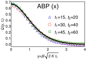
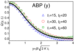
Refer to caption
Refer to caption
Figure 18: Comparision of the scaling relation in Eq. (161) for xπ‘₯x-coordinate (left panel) and y𝑦y-coordinate (right panel) of the ABP (shown by black line) with the same obtained from the numerical simulation (shown by symbols). For both plots, we have chosen K=2,vA=1.5,Dr​o​t=1formulae-sequence𝐾2formulae-sequencesubscript𝑣𝐴1.5subscriptπ·π‘Ÿπ‘œπ‘‘1K=2,~{}v_{A}=1.5,~{}D_{rot}=1 and N=100𝑁100N=100 for simulation.

6 Conclusions

To summarize, we have studied a chain of N𝑁N active particles with nearest neighbour quadratic interaction. We considered three models of active particles, namely, run and tumble particle, active Ornstein-Uhlenbeck particle and active Brownian particle. While the first two models are considered in one dimension, the ABP has been studied in two dimension. For all models, there exists three time scales - (i) Ο„K=1Ksubscript𝜏𝐾1𝐾\tau_{K}=\frac{1}{K} due to the interaction among particles, (ii) Ο„A=1ΞΆ/1Ξ³/1Dr​o​tsubscript𝜏𝐴1𝜁1𝛾1subscriptπ·π‘Ÿπ‘œπ‘‘\tau_{A}=\frac{1}{\zeta}~{}/\frac{1}{\gamma}~{}/\frac{1}{D_{rot}} due to the activity of RTPΒ /Β AOUPΒ /Β ABP. and (iii) Ο„N=N2Ksubscriptπœπ‘superscript𝑁2𝐾\tau_{N}=\frac{N^{2}}{K} due to the finiteness of the ring (note that Ο„Kβ‰ͺΟ„Aβ‰ͺΟ„Nmuch-less-thansubscript𝜏𝐾subscript𝜏𝐴much-less-thansubscriptπœπ‘\tau_{K}\ll\tau_{A}\ll\tau_{N} as shown in Fig. 2 ). We investigated various statistical quantities for the position of the tagged particles which were shown to exhibit interesting scaling structures depending on where the observation time t𝑑t lies. We emphasise that using our simple and analytically tractable model, we were able to re-derive many features which are seen in particles with non-trivial interactions.

We first looked at the MSD of the tagged particle’s position. For all models, there is a crossover of the MSD from super-diffusive scaling (∼tΞΌ)similar-toabsentsuperscriptπ‘‘πœ‡(\sim t^{\mu}) for tβ‰ͺΟ„Amuch-less-than𝑑subscript𝜏𝐴t\ll\tau_{A} to the sub-diffusive scaling (∼t)similar-toabsent𝑑(\sim\sqrt{t}) for t≫τAmuch-greater-than𝑑subscript𝜏𝐴t\gg\tau_{A} with ΞΌ=32πœ‡32\mu=\frac{3}{2} for RTP, ΞΌ=52πœ‡52\mu=\frac{5}{2} for AOUP, ΞΌ=72(=52)πœ‡annotated72absent52\mu=\frac{7}{2}~{}\left(=\frac{5}{2}\right) for x​(y)π‘₯𝑦x~{}(y)-coordinate of ABP. We analytically computed the crossover function that connects these two distinct scaling regimes in Eqs. (37) and (107) for RTP and AOUP respectively and in Eqs. (139) and (140) for ABP. Note that tΞΌsuperscriptπ‘‘πœ‡t^{\mu} scaling of the MSD arises due to the interplay of the activity and caging effect due to the surrounding particles. Furthermore, we also studied the MSD for tβˆΌΟ„Nsimilar-to𝑑subscriptπœπ‘t\sim\tau_{N} and showed that it exhibits crossover from t𝑑\sqrt{t} scaling for tβ‰ͺΟ„Nmuch-less-than𝑑subscriptπœπ‘t\ll\tau_{N} to the diffusive scaling for t≫τNmuch-greater-than𝑑subscriptπœπ‘t\gg\tau_{N} for all models. Here also, we explicitly computed the corresponding crossover function in Eq. (88). Such crossover behaviour for the MSD of active particles with hardcore repulsive interactions was predicted in [75] which we have rigorously derived in the simple setting of harmonic chain.

Next we studied the equal time two-point correlation function ⟨x0​(t)​xβ​(t)⟩csubscriptdelimited-⟨⟩subscriptπ‘₯0𝑑subscriptπ‘₯𝛽𝑑𝑐\langle x_{0}(t)x_{\beta}(t)\rangle_{c} for the two models. It was shown that ⟨x0​(t)​xβ​(t)⟩csubscriptdelimited-⟨⟩subscriptπ‘₯0𝑑subscriptπ‘₯𝛽𝑑𝑐\langle x_{0}(t)x_{\beta}(t)\rangle_{c} exhibits scaling forms with respect to y=Ξ²2​K​t𝑦𝛽2𝐾𝑑y=\frac{\beta}{\sqrt{2Kt}} with distinct scaling functions Ξ©R​T​(y)superscriptΩ𝑅𝑇𝑦\Omega^{RT}(y), Ξ©O​U​(y)superscriptΞ©π‘‚π‘ˆπ‘¦\Omega^{OU}(y) and Ξ©1/2A​B​(y)subscriptsuperscriptΩ𝐴𝐡12𝑦\Omega^{AB}_{1/2}(y) which were derived in Eqs. (47), (116), (159) and (160) respectively. On the other hand, all three models give rise to the same scaling form (as expected) for t≫τAmuch-greater-than𝑑subscript𝜏𝐴t\gg\tau_{A} with the corresponding scaling function π’žβ€‹(y)π’žπ‘¦\mathcal{C}(y) given in Eq. (51). In addition to these extreme limits, we also computed the correlation function when tβˆΌΟ„Asimilar-to𝑑subscript𝜏𝐴t\sim\tau_{A}.

We have also investigated the mean squared auto fluctuations ⟨xα​(t1)​xα​(t2)⟩csubscriptdelimited-⟨⟩subscriptπ‘₯𝛼subscript𝑑1subscriptπ‘₯𝛼subscript𝑑2𝑐\langle x_{\alpha}(t_{1})x_{\alpha}(t_{2})\rangle_{c} with t1≀t2subscript𝑑1subscript𝑑2t_{1}\leq t_{2}. Keeping the ratio tr=t2t1subscriptπ‘‘π‘Ÿsubscript𝑑2subscript𝑑1t_{r}=\frac{t_{2}}{t_{1}} fixed, we analysed the auto fluctuation for two different limits for t1subscript𝑑1t_{1} and t2subscript𝑑2t_{2} - (A) t1β‰ͺΟ„Amuch-less-thansubscript𝑑1subscript𝜏𝐴t_{1}\ll\tau_{A}, t2β‰ͺΟ„Amuch-less-thansubscript𝑑2subscript𝜏𝐴t_{2}\ll\tau_{A} and (B) t1≫τAmuch-greater-thansubscript𝑑1subscript𝜏𝐴t_{1}\gg\tau_{A}, t2≫τAmuch-greater-thansubscript𝑑2subscript𝜏𝐴t_{2}\gg\tau_{A}. For case (A), the three models exhibit distinct scaling functions β„’R​T​(tr)superscriptℒ𝑅𝑇subscriptπ‘‘π‘Ÿ\mathcal{L}^{RT}(t_{r}), β„’O​U​(tr)superscriptβ„’π‘‚π‘ˆsubscriptπ‘‘π‘Ÿ\mathcal{L}^{OU}(t_{r}) and β„’1/2A​B​(tr)subscriptsuperscriptℒ𝐴𝐡12subscriptπ‘‘π‘Ÿ\mathcal{L}^{AB}_{1/2}(t_{r}) which we have computed in Eqs. (61), (113), (155) and (156) respectively. However for case (B), all models converge to the same scaling function ℳ​(tr)β„³subscriptπ‘‘π‘Ÿ\mathcal{M}(t_{r}) in Eq. (67) for the auto correlation. We also showed that the auto correlation has a non-monotonic dependence on t2subscript𝑑2t_{2} in which ⟨xα​(t1)​xα​(t2)⟩csubscriptdelimited-⟨⟩subscriptπ‘₯𝛼subscript𝑑1subscriptπ‘₯𝛼subscript𝑑2𝑐\langle x_{\alpha}(t_{1})x_{\alpha}(t_{2})\rangle_{c} first increases with t2subscript𝑑2t_{2}, reaches a maximum value and then starts decreasing again. This non-monotonic nature of ⟨xα​(t1)​xα​(t2)⟩csubscriptdelimited-⟨⟩subscriptπ‘₯𝛼subscript𝑑1subscriptπ‘₯𝛼subscript𝑑2𝑐\langle x_{\alpha}(t_{1})x_{\alpha}(t_{2})\rangle_{c} is again the signature of the activity of the particles.

Finally, we studied the unequal time correlation function ⟨x0​(t1)​xβ​(t2)⟩csubscriptdelimited-⟨⟩subscriptπ‘₯0subscript𝑑1subscriptπ‘₯𝛽subscript𝑑2𝑐\langle x_{0}(t_{1})x_{\beta}(t_{2})\rangle_{c} (t1≀t2subscript𝑑1subscript𝑑2t_{1}\leq t_{2}) which also shows various scaling structures depending on where t1subscript𝑑1t_{1} and t2subscript𝑑2t_{2} lie. For case (A), ⟨x0​(t1)​xβ​(t2)⟩csubscriptdelimited-⟨⟩subscriptπ‘₯0subscript𝑑1subscriptπ‘₯𝛽subscript𝑑2𝑐\langle x_{0}(t_{1})x_{\beta}(t_{2})\rangle_{c} displays scaling form with respect to tr=t2t1subscriptπ‘‘π‘Ÿsubscript𝑑2subscript𝑑1t_{r}=\frac{t_{2}}{t_{1}} and y=Ξ²2​K​t1𝑦𝛽2𝐾subscript𝑑1y=\frac{\beta}{\sqrt{2Kt_{1}}} with the corresponding scaling functions 𝒫R​T​(y,tr)superscript𝒫𝑅𝑇𝑦subscriptπ‘‘π‘Ÿ\mathcal{P}^{RT}(y,t_{r}), 𝒫O​U​(y,tr)superscriptπ’«π‘‚π‘ˆπ‘¦subscriptπ‘‘π‘Ÿ\mathcal{P}^{OU}(y,t_{r}) and 𝒫1/2A​B​(y,tr)subscriptsuperscript𝒫𝐴𝐡12𝑦subscriptπ‘‘π‘Ÿ\mathcal{P}^{AB}_{1/2}(y,t_{r}) computed in Eqs. (77), (112), (150) and (152). For case (B), in conjunction to the previous cases, here also, the two models converge to the same scaling function 𝒬​(y,tr)𝒬𝑦subscriptπ‘‘π‘Ÿ\mathcal{Q}(y,t_{r}) given in Eq. (80). Interestingly, for a given β𝛽\beta, ⟨x0​(t1)​xβ​(t2)⟩csubscriptdelimited-⟨⟩subscriptπ‘₯0subscript𝑑1subscriptπ‘₯𝛽subscript𝑑2𝑐\langle x_{0}(t_{1})x_{\beta}(t_{2})\rangle_{c} also exhibits non-monotonic behaviour with respect to t2subscript𝑑2t_{2} in which it increases with t2subscript𝑑2t_{2}, attains a maximum and then starts decreasing again. Once again, this non-monotonic nature is the signature of the activity of the particles. A summary of results for all three models are given in Tables 1 and 2.

7 Acknowledgement

We thank Julien Cividini for fruitful discussions and important comments on the draft. AK and PS acknowledge support of the Department of Atomic Energy, Government of India, under project no.12-R&D-TFR-5.10-1100. AK acknowledges support from DST, Government of India grant under project No. ECR/2017/000634.

CΞ±1,Ξ±2​(t1,t2)=⟨xΞ±1​(t1)​xΞ±2​(t2)⟩csubscript𝐢subscript𝛼1subscript𝛼2subscript𝑑1subscript𝑑2subscriptdelimited-⟨⟩subscriptπ‘₯subscript𝛼1subscript𝑑1subscriptπ‘₯subscript𝛼2subscript𝑑2𝑐C_{\alpha_{1},\alpha_{2}}(t_{1},t_{2})=\langle x_{\alpha_{1}}(t_{1})x_{\alpha_{2}}(t_{2})\rangle_{c}
Quantities Model - RTPΒ /AOUP,Β Β Β  Ο„K=1K,Ο„A=1ΞΆ/1Ξ³formulae-sequencesubscript𝜏𝐾1𝐾subscript𝜏𝐴1𝜁1𝛾\tau_{K}=\frac{1}{K},~{}\tau_{A}=\frac{1}{\zeta}~{}/\frac{1}{\gamma} and Ο„N=N2Ksubscriptπœπ‘superscript𝑁2𝐾\tau_{N}=\frac{N^{2}}{K}.
MSD CΞ±,α​(t,t)subscript𝐢𝛼𝛼𝑑𝑑C_{\alpha,\alpha}(t,t) Nβ†’βˆžβ†’π‘N\to\infty Time β‰ͺΟ„Kmuch-less-thanabsentsubscript𝜏𝐾\ll\tau_{K} Time ≫τKmuch-greater-thanabsentsubscript𝜏𝐾\gg\tau_{K}
\addstackgap[.5]() ≃{v02​t2,Β (RTP)2​D3​t3,Β (AOUP)similar-to-or-equalsabsentcasessuperscriptsubscript𝑣02superscript𝑑2Β (RTP)otherwise2𝐷3superscript𝑑3Β (AOUP)otherwise\simeq\begin{cases}v_{0}^{2}t^{2},\text{ (RTP)}\\ \frac{2D}{3}t^{3},\text{ (AOUP)}\end{cases} ∼t3/2​𝒯R​T/O​U​(tΟ„A)similar-toabsentsuperscript𝑑32superscriptπ’―π‘…π‘‡π‘‚π‘ˆπ‘‘subscript𝜏𝐴\sim t^{3/2}~{}\mathcal{T}^{RT/OU}\left(\frac{t}{\tau_{A}}\right)
Eqs.Β (35) and (104) with Ο„A=1ΞΆ/1Ξ³subscript𝜏𝐴1𝜁1𝛾\tau_{A}=\frac{1}{\zeta}~{}/\frac{1}{\gamma} for RTP /AOUP,
see Eqs.Β (36) and (106)
\addstackgap[.5]() Large but finite N𝑁N ≃2​De​f​f​NK​Φ​(K​tN2)similar-to-or-equalsabsent2subscript𝐷𝑒𝑓𝑓𝑁𝐾Φ𝐾𝑑superscript𝑁2\simeq\frac{2D_{eff}N}{K}\Phi\left(\frac{Kt}{N^{2}}\right)
where Φ​(y)=y+βˆ‘s=1∞1βˆ’exp​(βˆ’8​π2​s2​y)4​π2​s2Φ𝑦𝑦superscriptsubscript𝑠11exp8superscriptπœ‹2superscript𝑠2𝑦4superscriptπœ‹2superscript𝑠2\Phi(y)=y+\sum_{s=1}^{\infty}\frac{1-\text{exp}({-8\pi^{2}s^{2}y})}{4\pi^{2}s^{2}}
and De​f​f=DR/DAsubscript𝐷𝑒𝑓𝑓subscript𝐷𝑅subscript𝐷𝐴D_{eff}=D_{R}~{}/D_{A} for RTPΒ /AOUP
Covariance C0,β​(t,t)subscript𝐢0𝛽𝑑𝑑C_{0,\beta}(t,t) Nβ†’βˆžβ†’π‘N\to\infty Time β‰ͺΟ„Kmuch-less-thanabsentsubscript𝜏𝐾\ll\tau_{K} Time ≫τKmuch-greater-thanabsentsubscript𝜏𝐾\gg\tau_{K}
\addstackgap[.5]() ≃δ0,β​{v02​t2,(RTP)2​D3​t3​(AOUP)similar-to-or-equalsabsentsubscript𝛿0𝛽casessuperscriptsubscript𝑣02superscript𝑑2(RTP)otherwise2𝐷3superscript𝑑3(AOUP)otherwise\simeq\delta_{0,\beta}\begin{cases}v_{0}^{2}t^{2},~{}\text{(RTP)}\\ \frac{2D}{3}t^{3}~{}\text{(AOUP)}\end{cases} ∼{tμ​ΩR​T/O​U​(Ξ²2​K​t);tβ‰ͺΟ„Atβ€‹π’žβ€‹(Ξ²2​K​t);t≫τA\sim\begin{cases}t^{\mu}~{}\Omega^{RT/OU}\left(\frac{\beta}{\sqrt{2Kt}}\right)\\ ~{}~{}~{}~{}~{}~{}~{}~{}~{};~{}t\ll\tau_{A}\\ \sqrt{t}~{}\mathcal{C}\left(\frac{\beta}{\sqrt{2Kt}}\right)\\ ~{}~{}~{}~{}~{}~{}~{}~{}~{}~{};~{}t\gg\tau_{A}\end{cases}
ΞΌ=32/52πœ‡3252\mu=\frac{3}{2}~{}/\frac{5}{2} for RTP/AOUP, see
Eqs.Β (47) and (115) for Ξ©R​T/O​U​(y)superscriptΞ©π‘…π‘‡π‘‚π‘ˆπ‘¦\Omega^{RT/OU}(y)
and Eq.Β (51) for π’žβ€‹(y)π’žπ‘¦\mathcal{C}(y).
\addstackgap[.5]() Large but finite N𝑁N ≃2​De​f​f​NK​Ψ​(Ξ²N,K​tN2)similar-to-or-equalsabsent2subscript𝐷𝑒𝑓𝑓𝑁𝐾Ψ𝛽𝑁𝐾𝑑superscript𝑁2\simeq\frac{2D_{eff}N}{K}\Psi\left(\frac{\beta}{N},\frac{Kt}{N^{2}}\right) where,
where Ψ​(z,y)=y+βˆ‘s=1∞cos⁑(2​π​s​z)​1βˆ’exp​(βˆ’8​π2​s2​y)4​π2​s2Ψ𝑧𝑦𝑦superscriptsubscript𝑠12πœ‹π‘ π‘§1exp8superscriptπœ‹2superscript𝑠2𝑦4superscriptπœ‹2superscript𝑠2\Psi(z,y)=y+\sum_{s=1}^{\infty}\cos(2\pi sz)\frac{1-\text{exp}({-8\pi^{2}s^{2}y})}{4\pi^{2}s^{2}}
and De​f​f=DR/DAsubscript𝐷𝑒𝑓𝑓subscript𝐷𝑅subscript𝐷𝐴D_{eff}=D_{R}~{}/D_{A} for RTPΒ /AOUP
Position Auto Correlation CΞ±,α​(t1,t2)subscript𝐢𝛼𝛼subscript𝑑1subscript𝑑2C_{\alpha,\alpha}(t_{1},t_{2}) Nβ†’βˆžβ†’π‘N\to\infty Time β‰ͺΟ„Kmuch-less-thanabsentsubscript𝜏𝐾\ll\tau_{K} Time ≫τKmuch-greater-thanabsentsubscript𝜏𝐾\gg\tau_{K}
\addstackgap[.5]() ≃{v02​t1​t2​(RTP)D​t12​(t2βˆ’t13)(AOUP)similar-to-or-equalsabsentcasessuperscriptsubscript𝑣02subscript𝑑1subscript𝑑2(RTP)otherwise𝐷superscriptsubscript𝑑12subscript𝑑2subscript𝑑13otherwise(AOUP)otherwise\simeq\begin{cases}v_{0}^{2}t_{1}t_{2}~{}\text{(RTP)}\\ Dt_{1}^{2}\left(t_{2}-\frac{t_{1}}{3}\right)\\ ~{}\text{(AOUP)}\end{cases} ∼{t1μ​ℒR​T/O​U​(t2t1);t1≀t2β‰ͺΟ„At1​ℳ​(t2t1);Ο„Aβ‰ͺt1≀t2\sim\begin{cases}t_{1}^{\mu}~{}\mathcal{L}^{RT/OU}\left(\frac{t_{2}}{t_{1}}\right)\\ ~{}~{}~{}~{}~{}~{}~{}~{}~{}~{}~{}~{};~{}t_{1}\leq t_{2}\ll\tau_{A}\\ \sqrt{t_{1}}~{}\mathcal{M}\left(\frac{t_{2}}{t_{1}}\right)\\ ~{}~{}~{}~{}~{}~{}~{}~{}~{}~{}~{}~{};~{}\tau_{A}\ll t_{1}\leq t_{2}\end{cases}
ΞΌ=32/52πœ‡3252\mu=\frac{3}{2}~{}/\frac{5}{2} for RTP/AOUP, see
Eqs. (61) and (113) for β„’R​T/O​U​(tr)superscriptβ„’π‘…π‘‡π‘‚π‘ˆsubscriptπ‘‘π‘Ÿ\mathcal{L}^{RT/OU}(t_{r})
and Eq. (67) for ℳ​(tr)β„³subscriptπ‘‘π‘Ÿ\mathcal{M}(t_{r})
\addstackgap[.5]() Large but finite N𝑁N ≃2​De​f​f​NK​ℛ​(t2t1,K​tN2)similar-to-or-equalsabsent2subscript𝐷𝑒𝑓𝑓𝑁𝐾ℛsubscript𝑑2subscript𝑑1𝐾𝑑superscript𝑁2\simeq\frac{2D_{eff}N}{K}\mathcal{R}\left(\frac{t_{2}}{t_{1}},\frac{Kt}{N^{2}}\right) where,
where ℛ​(tr,y)=y+βˆ‘s=1∞eβˆ’4​π2​s2​y​tr​Sinh​(4​π2​s2​y)2​π2​s2β„›subscriptπ‘‘π‘Ÿπ‘¦π‘¦superscriptsubscript𝑠1superscripte4superscriptπœ‹2superscript𝑠2𝑦subscriptπ‘‘π‘ŸSinh4superscriptπœ‹2superscript𝑠2𝑦2superscriptπœ‹2superscript𝑠2\mathcal{R}(t_{r},y)=y+\sum_{s=1}^{\infty}\text{e}^{-4\pi^{2}s^{2}yt_{r}}\frac{\text{Sinh}\left({4\pi^{2}s^{2}y}\right)}{2\pi^{2}s^{2}}
and De​f​f=DR/DAsubscript𝐷𝑒𝑓𝑓subscript𝐷𝑅subscript𝐷𝐴D_{eff}=D_{R}~{}/D_{A} for RTPΒ /AOUP.
CΞ±1,Ξ±2​(t1,t2)=⟨xΞ±1​(t1)​xΞ±2​(t2)⟩csubscript𝐢subscript𝛼1subscript𝛼2subscript𝑑1subscript𝑑2subscriptdelimited-⟨⟩subscriptπ‘₯subscript𝛼1subscript𝑑1subscriptπ‘₯subscript𝛼2subscript𝑑2𝑐C_{\alpha_{1},\alpha_{2}}(t_{1},t_{2})=\langle x_{\alpha_{1}}(t_{1})x_{\alpha_{2}}(t_{2})\rangle_{c}
Quantities Model - RTP /AOUP,Β Β Β Ο„K=1K,Ο„A=1ΞΆ/1Ξ³formulae-sequencesubscript𝜏𝐾1𝐾subscript𝜏𝐴1𝜁1𝛾\tau_{K}=\frac{1}{K},~{}\tau_{A}=\frac{1}{\zeta}~{}/\frac{1}{\gamma} and Ο„N=N2Ksubscriptπœπ‘superscript𝑁2𝐾\tau_{N}=\frac{N^{2}}{K}.
Unequal time correlation C0,β​(t1,t2)subscript𝐢0𝛽subscript𝑑1subscript𝑑2C_{0,\beta}(t_{1},t_{2}) Nβ†’βˆžβ†’π‘N\to\infty Time β‰ͺΟ„Kmuch-less-thanabsentsubscript𝜏𝐾\ll\tau_{K} Time ≫τKmuch-greater-thanabsentsubscript𝜏𝐾\gg\tau_{K}
≃δβ,0​{v02​t1​t2​(RTP)D​t12​(t2βˆ’t13)(AOUP)similar-to-or-equalsabsentsubscript𝛿𝛽0casessuperscriptsubscript𝑣02subscript𝑑1subscript𝑑2(RTP)otherwise𝐷superscriptsubscript𝑑12subscript𝑑2subscript𝑑13otherwise(AOUP)otherwise\simeq\delta_{\beta,0}\begin{cases}v_{0}^{2}t_{1}t_{2}~{}\text{(RTP)}\\ Dt_{1}^{2}\left(t_{2}-\frac{t_{1}}{3}\right)\\ ~{}\text{(AOUP)}\end{cases} ∼{t1μ​𝒫R​T/O​U​(Ξ²2​K​t1,t2t1);t1≀t2β‰ͺΟ„At1​𝒬​(Ξ²2​K​t1,t2t1);Ο„Aβ‰ͺt1≀t2\sim\begin{cases}t_{1}^{\mu}~{}\mathcal{P}^{RT/OU}\left(\frac{\beta}{\sqrt{2Kt_{1}}},\frac{t_{2}}{t_{1}}\right)\\ ~{}~{}~{}~{}~{}~{}~{}~{}~{}~{}~{}~{};~{}t_{1}\leq t_{2}\ll\tau_{A}\\ \sqrt{t_{1}}~{}\mathcal{Q}\left(\frac{\beta}{\sqrt{2Kt_{1}}},\frac{t_{2}}{t_{1}}\right)\\ ~{}~{}~{}~{}~{}~{}~{}~{}~{}~{}~{}~{};~{}\tau_{A}\ll t_{1}\leq t_{2}\end{cases}
ΞΌ=32/52πœ‡3252\mu=\frac{3}{2}~{}/\frac{5}{2} for RTP/AOUP, see
Eqs.Β (77) and (112) for 𝒫R​T/O​U​(y,tr)superscriptπ’«π‘…π‘‡π‘‚π‘ˆπ‘¦subscriptπ‘‘π‘Ÿ\mathcal{P}^{RT/OU}(y,t_{r})
and Eq.Β (80) for 𝒬​(y,tr)𝒬𝑦subscriptπ‘‘π‘Ÿ\mathcal{Q}(y,t_{r}).
\addstackgap[.5]() Large but finite N𝑁N ≃2​De​f​f​NK​𝒲​(t2t1,Ξ²N,K​t1N2)similar-to-or-equalsabsent2subscript𝐷𝑒𝑓𝑓𝑁𝐾𝒲subscript𝑑2subscript𝑑1𝛽𝑁𝐾subscript𝑑1superscript𝑁2\simeq\frac{2D_{eff}N}{K}~{}\mathcal{W}\left(\frac{t_{2}}{t_{1}},\frac{\beta}{N},\frac{Kt_{1}}{N^{2}}\right) where,
where 𝒲​(tr,z,y)=y+βˆ‘s=1∞cos⁑(2​π​s​z)​eβˆ’4​π2​s2​y​tr​Sinh​(4​π2​s2​y)2​π2​s2𝒲subscriptπ‘‘π‘Ÿπ‘§π‘¦π‘¦superscriptsubscript𝑠12πœ‹π‘ π‘§superscripte4superscriptπœ‹2superscript𝑠2𝑦subscriptπ‘‘π‘ŸSinh4superscriptπœ‹2superscript𝑠2𝑦2superscriptπœ‹2superscript𝑠2\mathcal{W}(t_{r},z,y)=y+\sum_{s=1}^{\infty}\cos\left(2\pi sz\right)\text{e}^{-4\pi^{2}s^{2}yt_{r}}\frac{\text{Sinh}\left({4\pi^{2}s^{2}y}\right)}{2\pi^{2}s^{2}}
and De​f​f=DR/DAsubscript𝐷𝑒𝑓𝑓subscript𝐷𝑅subscript𝐷𝐴D_{eff}=D_{R}~{}/D_{A} for RTPΒ /AOUP.
Table 1: Summary of the results on two-point position correlations in the harmonic chain of RTP and AOUP.
CΞ±1,Ξ±21​(t1,t2)=⟨xΞ±1​(t1)​xΞ±2​(t2)⟩csubscriptsuperscript𝐢1subscript𝛼1subscript𝛼2subscript𝑑1subscript𝑑2subscriptdelimited-⟨⟩subscriptπ‘₯subscript𝛼1subscript𝑑1subscriptπ‘₯subscript𝛼2subscript𝑑2𝑐C^{1}_{\alpha_{1},\alpha_{2}}(t_{1},t_{2})=\langle x_{\alpha_{1}}(t_{1})x_{\alpha_{2}}(t_{2})\rangle_{c}
CΞ±1,Ξ±22​(t1,t2)=⟨yΞ±1​(t1)​yΞ±2​(t2)⟩csubscriptsuperscript𝐢2subscript𝛼1subscript𝛼2subscript𝑑1subscript𝑑2subscriptdelimited-⟨⟩subscript𝑦subscript𝛼1subscript𝑑1subscript𝑦subscript𝛼2subscript𝑑2𝑐C^{2}_{\alpha_{1},\alpha_{2}}(t_{1},t_{2})=\langle y_{\alpha_{1}}(t_{1})y_{\alpha_{2}}(t_{2})\rangle_{c}
Quantities Model - ABP,Β Β Β  Ο„K=1K,Ο„A=1Dr​o​tformulae-sequencesubscript𝜏𝐾1𝐾subscript𝜏𝐴1subscriptπ·π‘Ÿπ‘œπ‘‘\tau_{K}=\frac{1}{K},~{}\tau_{A}=\frac{1}{D_{rot}} and Ο„N=N2Ksubscriptπœπ‘superscript𝑁2𝐾\tau_{N}=\frac{N^{2}}{K}.
MSD CΞ±,Ξ±p​(t,t)superscriptsubscript𝐢𝛼𝛼𝑝𝑑𝑑C_{\alpha,\alpha}^{p}(t,t) Nβ†’βˆžβ†’π‘N\to\infty Time β‰ͺΟ„Kmuch-less-thanabsentsubscript𝜏𝐾\ll\tau_{K} Time ≫τKmuch-greater-thanabsentsubscript𝜏𝐾\gg\tau_{K}
\addstackgap[.5]() ∼{t4,p=1t3,p=2similar-toabsentcasessuperscript𝑑4𝑝1otherwisesuperscript𝑑3𝑝2otherwise\sim\begin{cases}t^{4},~{}~{}~{}p=1\\ t^{3},~{}~{}~{}p=2\end{cases} ∼t3/2​𝒯pA​B​(Dr​o​t​t)similar-toabsentsuperscript𝑑32superscriptsubscript𝒯𝑝𝐴𝐡subscriptπ·π‘Ÿπ‘œπ‘‘π‘‘\sim t^{3/2}~{}\mathcal{T}_{p}^{AB}\left(D_{rot}t\right)
see Eqs.Β (133) and (134) see Eqs.Β (137) and (138)
\addstackgap[.5]() Large but finite N𝑁N ≃2​DA​B​P​NK​Φ​(K​tN2)similar-to-or-equalsabsent2subscript𝐷𝐴𝐡𝑃𝑁𝐾Φ𝐾𝑑superscript𝑁2\simeq\frac{2D_{ABP}N}{K}\Phi\left(\frac{Kt}{N^{2}}\right)
Φ​(z,y)=y+βˆ‘s=1∞1βˆ’exp​(βˆ’8​π2​s2​y)4​π2​s2Φ𝑧𝑦𝑦superscriptsubscript𝑠11exp8superscriptπœ‹2superscript𝑠2𝑦4superscriptπœ‹2superscript𝑠2\Phi(z,y)=y+\sum_{s=1}^{\infty}\frac{1-\text{exp}({-8\pi^{2}s^{2}y})}{4\pi^{2}s^{2}}
Covariance C0,Ξ²p​(t,t)superscriptsubscript𝐢0𝛽𝑝𝑑𝑑C_{0,\beta}^{p}(t,t) Nβ†’βˆžβ†’π‘N\to\infty Time β‰ͺΟ„Kmuch-less-thanabsentsubscript𝜏𝐾\ll\tau_{K} Time ≫τKmuch-greater-thanabsentsubscript𝜏𝐾\gg\tau_{K}
\addstackgap[.5]() ∼{t4​δ0,Ξ²,p=1t3​δ0,Ξ²,p=2similar-toabsentcasessuperscript𝑑4subscript𝛿0𝛽𝑝1otherwisesuperscript𝑑3subscript𝛿0𝛽𝑝2otherwise\sim\begin{cases}t^{4}\delta_{0,\beta},~{}~{}p=1\\ t^{3}\delta_{0,\beta},~{}~{}p=2\end{cases} ∼{tν​ΩpA​B​(Ξ²2​K​t);tβ‰ͺΟ„Atβ€‹π’žβ€‹(Ξ²2​K​t);t≫τA\sim\begin{cases}t^{\nu}~{}\Omega^{AB}_{p}\left(\frac{\beta}{\sqrt{2Kt}}\right)\\ ~{}~{}~{}~{}~{}~{}~{}~{}~{};~{}t\ll\tau_{A}\\ {\sqrt{t}~{}\mathcal{C}\left(\frac{\beta}{\sqrt{2Kt}}\right)}\\ ~{}~{}~{}~{}~{}~{}~{}~{}~{}~{};~{}t\gg\tau_{A}\end{cases}
see Eqs.Β (133) and (134) where Ξ½=72/52𝜈7252\nu=\frac{7}{2}~{}/\frac{5}{2} for p=1/2𝑝12p=1/2,
Ξ©1/2A​B​(y)superscriptsubscriptΞ©12𝐴𝐡𝑦\Omega_{1/2}^{AB}(y) are given in
Eqs.Β (159) and (160)
and π’žβ€‹(y)π’žπ‘¦\mathcal{C}(y) in Eq.Β (51).
\addstackgap[.5]() Large but finite N𝑁N ≃2​DA​B​P​NK​Ψ​(Ξ²N,K​tN2)similar-to-or-equalsabsent2subscript𝐷𝐴𝐡𝑃𝑁𝐾Ψ𝛽𝑁𝐾𝑑superscript𝑁2\simeq\frac{2D_{ABP}N}{K}\Psi\left(\frac{\beta}{N},\frac{Kt}{N^{2}}\right) where,
Ψ​(z,y)=y+βˆ‘s=1∞cos⁑(2​π​s​z)​1βˆ’exp​(βˆ’8​π2​s2​y)4​π2​s2Ψ𝑧𝑦𝑦superscriptsubscript𝑠12πœ‹π‘ π‘§1exp8superscriptπœ‹2superscript𝑠2𝑦4superscriptπœ‹2superscript𝑠2\Psi(z,y)=y+\sum_{s=1}^{\infty}\cos(2\pi sz)\frac{1-\text{exp}({-8\pi^{2}s^{2}y})}{4\pi^{2}s^{2}}
Position Auto Correlation CΞ±,Ξ±p​(t1,t2)subscriptsuperscript𝐢𝑝𝛼𝛼subscript𝑑1subscript𝑑2C^{p}_{\alpha,\alpha}(t_{1},t_{2}) Nβ†’βˆžβ†’π‘N\to\infty Time β‰ͺΟ„Kmuch-less-thanabsentsubscript𝜏𝐾\ll\tau_{K} Time ≫τKmuch-greater-thanabsentsubscript𝜏𝐾\gg\tau_{K}
\addstackgap[.5]() ∼{t13​(2​t2βˆ’t1),p=1t12​(t2βˆ’t13),p=2similar-toabsentcasessuperscriptsubscript𝑑132subscript𝑑2subscript𝑑1𝑝1otherwisesuperscriptsubscript𝑑12subscript𝑑2subscript𝑑13𝑝2otherwise\sim\begin{cases}t_{1}^{3}(2t_{2}-t_{1}),~{}~{}p=1\\ t_{1}^{2}\left(t_{2}-\frac{t_{1}}{3}\right),~{}~{}p=2\end{cases} ∼{t1ν​ℒpA​B​(t2t1);t1≀t2β‰ͺΟ„At1​ℳ​(t2t1);Ο„Aβ‰ͺt1≀t2\sim\begin{cases}t_{1}^{\nu}~{}\mathcal{L}^{AB}_{p}\left(\frac{t_{2}}{t_{1}}\right)\\ ~{}~{}~{}~{}~{}~{}~{}~{}~{};~{}t_{1}\leq t_{2}\ll\tau_{A}\\ {\sqrt{t_{1}}~{}\mathcal{M}\left(\frac{t_{2}}{t_{1}}\right)}\\ ~{}~{}~{}~{}~{}~{}~{}~{}~{};~{}\tau_{A}\ll t_{1}\leq t_{2}\end{cases}
see Eqs.Β (133) and (134) Ξ½=72/52𝜈7252\nu=\frac{7}{2}~{}/\frac{5}{2} for p=1/2𝑝12p=1/2, ℳ​(tr)β„³subscriptπ‘‘π‘Ÿ\mathcal{M}(t_{r})
is in Eq.Β (67) and β„’pA​B​(tr)subscriptsuperscriptℒ𝐴𝐡𝑝subscriptπ‘‘π‘Ÿ\mathcal{L}^{AB}_{p}(t_{r})
are in Eqs. (155) and (156).
\addstackgap[.5]() Large but finite N𝑁N ≃2​DA​B​P​NK​ℛ​(t2t1,K​tN2)similar-to-or-equalsabsent2subscript𝐷𝐴𝐡𝑃𝑁𝐾ℛsubscript𝑑2subscript𝑑1𝐾𝑑superscript𝑁2\simeq\frac{2D_{ABP}N}{K}\mathcal{R}\left(\frac{t_{2}}{t_{1}},\frac{Kt}{N^{2}}\right) where,
ℛ​(tr,y)=y+βˆ‘s=1∞eβˆ’4​π2​s2​y​tr​Sinh​(4​π2​s2​y)2​π2​s2β„›subscriptπ‘‘π‘Ÿπ‘¦π‘¦superscriptsubscript𝑠1superscripte4superscriptπœ‹2superscript𝑠2𝑦subscriptπ‘‘π‘ŸSinh4superscriptπœ‹2superscript𝑠2𝑦2superscriptπœ‹2superscript𝑠2\mathcal{R}(t_{r},y)=y+\sum_{s=1}^{\infty}\text{e}^{-4\pi^{2}s^{2}yt_{r}}\frac{\text{Sinh}\left({4\pi^{2}s^{2}y}\right)}{2\pi^{2}s^{2}}
CΞ±1,Ξ±21​(t1,t2)=⟨xΞ±1​(t1)​xΞ±2​(t2)⟩csubscriptsuperscript𝐢1subscript𝛼1subscript𝛼2subscript𝑑1subscript𝑑2subscriptdelimited-⟨⟩subscriptπ‘₯subscript𝛼1subscript𝑑1subscriptπ‘₯subscript𝛼2subscript𝑑2𝑐C^{1}_{\alpha_{1},\alpha_{2}}(t_{1},t_{2})=\langle x_{\alpha_{1}}(t_{1})x_{\alpha_{2}}(t_{2})\rangle_{c}
CΞ±1,Ξ±22​(t1,t2)=⟨yΞ±1​(t1)​yΞ±2​(t2)⟩csubscriptsuperscript𝐢2subscript𝛼1subscript𝛼2subscript𝑑1subscript𝑑2subscriptdelimited-⟨⟩subscript𝑦subscript𝛼1subscript𝑑1subscript𝑦subscript𝛼2subscript𝑑2𝑐C^{2}_{\alpha_{1},\alpha_{2}}(t_{1},t_{2})=\langle y_{\alpha_{1}}(t_{1})y_{\alpha_{2}}(t_{2})\rangle_{c}
Quantities Model - ABP,Β Β Β Ο„K=1K,Ο„A=1Dr​o​tformulae-sequencesubscript𝜏𝐾1𝐾subscript𝜏𝐴1subscriptπ·π‘Ÿπ‘œπ‘‘\tau_{K}=\frac{1}{K},~{}\tau_{A}=\frac{1}{D_{rot}} and Ο„N=N2Ksubscriptπœπ‘superscript𝑁2𝐾\tau_{N}=\frac{N^{2}}{K}.
Unequal time correlation C0,Ξ²p​(t1,t2)superscriptsubscript𝐢0𝛽𝑝subscript𝑑1subscript𝑑2C_{0,\beta}^{p}(t_{1},t_{2}) Nβ†’βˆžβ†’π‘N\to\infty Time β‰ͺΟ„Kmuch-less-thanabsentsubscript𝜏𝐾\ll\tau_{K} Time ≫τKmuch-greater-thanabsentsubscript𝜏𝐾\gg\tau_{K}
{∼t13​(2​t2βˆ’t1)​δβ,0,for ​p=1∼t12​(t2βˆ’t13)​δβ,0,for ​p=2casessimilar-toabsentsuperscriptsubscript𝑑132subscript𝑑2subscript𝑑1subscript𝛿𝛽0otherwisefor 𝑝1otherwisesimilar-toabsentsuperscriptsubscript𝑑12subscript𝑑2subscript𝑑13subscript𝛿𝛽0otherwisefor 𝑝2otherwise\begin{cases}\sim t_{1}^{3}(2t_{2}-t_{1})\delta_{\beta,0},\\ ~{}~{}~{}~{}~{}\text{for }p=1\\ \sim t_{1}^{2}\left(t_{2}-\frac{t_{1}}{3}\right)\delta_{\beta,0},\\ ~{}~{}~{}~{}~{}\text{for }p=2\end{cases} ∼{t1ν​𝒫pA​B​(Ξ²2​K​t1,t2t1);t1≀t2β‰ͺΟ„At1​𝒬​(Ξ²2​K​t1,t2t1);Ο„Aβ‰ͺt1≀t2\sim\begin{cases}t_{1}^{\nu}~{}\mathcal{P}^{AB}_{p}\left(\frac{\beta}{\sqrt{2Kt_{1}}},\frac{t_{2}}{t_{1}}\right)\\ ~{}~{}~{}~{}~{}~{}~{}~{}~{}~{}~{}~{};~{}t_{1}\leq t_{2}\ll\tau_{A}\\ \sqrt{t_{1}}~{}\mathcal{Q}\left(\frac{\beta}{\sqrt{2Kt_{1}}},\frac{t_{2}}{t_{1}}\right)\\ ~{}~{}~{}~{}~{}~{}~{}~{}~{}~{}~{}~{};~{}\tau_{A}\ll t_{1}\leq t_{2}\end{cases}
where Ξ½=72/52𝜈7252\nu=\frac{7}{2}~{}/\frac{5}{2} for p=1/2𝑝12p=1/2,
𝒬​(y,tr)𝒬𝑦subscriptπ‘‘π‘Ÿ\mathcal{Q}(y,t_{r}) is in Eq.Β (79) and
see Eqs.Β (133) and (134) 𝒫pA​B​(y,tr)subscriptsuperscript𝒫𝐴𝐡𝑝𝑦subscriptπ‘‘π‘Ÿ\mathcal{P}^{AB}_{p}(y,t_{r}) are in Eqs.Β (150)
and (152).
\addstackgap[.5]() Large but finite N𝑁N ≃2​DA​B​P​NK​𝒲​(t2t1,Ξ²N,K​t1N2)similar-to-or-equalsabsent2subscript𝐷𝐴𝐡𝑃𝑁𝐾𝒲subscript𝑑2subscript𝑑1𝛽𝑁𝐾subscript𝑑1superscript𝑁2\simeq\frac{2D_{ABP}N}{K}~{}\mathcal{W}\left(\frac{t_{2}}{t_{1}},\frac{\beta}{N},\frac{Kt_{1}}{N^{2}}\right) where,
𝒲​(tr,z,y)=y+βˆ‘s=1∞cos⁑(2​π​s​z)​eβˆ’4​π2​s2​y​tr​Sinh​(4​π2​s2​y)2​π2​s2𝒲subscriptπ‘‘π‘Ÿπ‘§π‘¦π‘¦superscriptsubscript𝑠12πœ‹π‘ π‘§superscripte4superscriptπœ‹2superscript𝑠2𝑦subscriptπ‘‘π‘ŸSinh4superscriptπœ‹2superscript𝑠2𝑦2superscriptπœ‹2superscript𝑠2\mathcal{W}(t_{r},z,y)=y+\sum_{s=1}^{\infty}\cos\left(2\pi sz\right)\text{e}^{-4\pi^{2}s^{2}yt_{r}}\frac{\text{Sinh}\left({4\pi^{2}s^{2}y}\right)}{2\pi^{2}s^{2}}
Table 2: Summary of the results on two-point position correlations in the harmonic chain of ABP.

Appendix A Computation of ⟨xΒ―s​(t)​xΒ―sβ€²βˆ—β€‹(t)⟩csubscriptdelimited-⟨⟩subscriptΒ―π‘₯𝑠𝑑superscriptsubscriptΒ―π‘₯superscript𝑠′𝑑𝑐\langle\bar{x}_{s}(t)\bar{x}_{s^{\prime}}^{*}(t)\rangle_{c} in Eqs. (30) and (99)

In this appendix, we will compute ⟨xΒ―s​(t)​xΒ―sβ€²βˆ—β€‹(t)⟩csubscriptdelimited-⟨⟩subscriptΒ―π‘₯𝑠𝑑superscriptsubscriptΒ―π‘₯superscript𝑠′𝑑𝑐\langle\bar{x}_{s}(t)\bar{x}_{s^{\prime}}^{*}(t)\rangle_{c} given in Eqs. (30) and (99) for RTPs and AOUPs respectively. To begin with, we rewrite FΒ―sA​(t)subscriptsuperscript¯𝐹𝐴𝑠𝑑\bar{F}^{A}_{s}(t) given by Eq. (25) as

FΒ―sA​(t)=1Nβ€‹βˆ‘Ξ±=0Nβˆ’1eβˆ’2​π​i​sN​α​FΞ±A​(t).subscriptsuperscript¯𝐹𝐴𝑠𝑑1𝑁superscriptsubscript𝛼0𝑁1superscript𝑒2πœ‹π‘–π‘ π‘π›Όsuperscriptsubscript𝐹𝛼𝐴𝑑\displaystyle\bar{F}^{A}_{s}(t)=\frac{1}{N}\sum_{\alpha=0}^{N-1}e^{-\frac{2\pi is}{N}\alpha}~{}F_{\alpha}^{A}(t). (163)

The unequal time correlation is given by ,

⟨FΒ―sA​(Ο„1)​FΒ―sβ€²Aβˆ—β€‹(Ο„2)⟩c=βˆ‘Ξ±=1Nβˆ’1eβˆ’2​π​i​αN​(sβˆ’sβ€²)β€‹βŸ¨FΞ±A​(Ο„1)​FΞ²#​(Ο„2)⟩c.subscriptdelimited-⟨⟩subscriptsuperscript¯𝐹𝐴𝑠subscript𝜏1subscriptsuperscript¯𝐹superscript𝐴superscript𝑠′subscript𝜏2𝑐superscriptsubscript𝛼1𝑁1superscript𝑒2πœ‹π‘–π›Όπ‘π‘ superscript𝑠′subscriptdelimited-⟨⟩subscriptsuperscript𝐹𝐴𝛼subscript𝜏1subscriptsuperscript𝐹#𝛽subscript𝜏2𝑐\displaystyle\langle\bar{F}^{A}_{s}(\tau_{1})\bar{F}^{A^{*}}_{s^{\prime}}(\tau_{2})\rangle_{c}=\sum_{\alpha=1}^{N-1}e^{-\frac{2\pi i\alpha}{N}(s-s^{\prime})}~{}\langle F^{A}_{\alpha}(\tau_{1})F^{\#}_{\beta}(\tau_{2})\rangle_{c}. (164)

where FΒ―sβ€²#β£βˆ—β€‹(Ο„2)subscriptsuperscript¯𝐹#superscript𝑠′subscript𝜏2\bar{F}^{\#~{}*}_{s^{\prime}}(\tau_{2}) is the complex conjugate of FΒ―sβ€²#​(Ο„2)subscriptsuperscript¯𝐹#superscript𝑠′subscript𝜏2\bar{F}^{\#}_{s^{\prime}}(\tau_{2}).

A.1 For RTP

Recall for RTP, FΞ±R​T​P​(t)=v0​σα​(t)superscriptsubscript𝐹𝛼𝑅𝑇𝑃𝑑subscript𝑣0subscriptπœŽπ›Όπ‘‘F_{\alpha}^{RTP}(t)=v_{0}\sigma_{\alpha}(t) as shown in Eq. (3). Substituting this in Eq. (164),

⟨FΒ―sR​T​P​(Ο„1)​FΒ―sβ€²R​T​Pβ£βˆ—β€‹(Ο„2)⟩c=v02N2β€‹βˆ‘Ξ±,Ξ²=1Nβˆ’1eβˆ’2​π​iN​(sβ€‹Ξ±βˆ’s′​β)β€‹βŸ¨ΟƒΞ±β€‹(Ο„1)​σβ​(Ο„2)⟩c,subscriptdelimited-⟨⟩subscriptsuperscript¯𝐹𝑅𝑇𝑃𝑠subscript𝜏1subscriptsuperscript¯𝐹𝑅𝑇𝑃superscript𝑠′subscript𝜏2𝑐superscriptsubscript𝑣02superscript𝑁2superscriptsubscript𝛼𝛽1𝑁1superscript𝑒2πœ‹π‘–π‘π‘ π›Όsuperscript𝑠′𝛽subscriptdelimited-⟨⟩subscriptπœŽπ›Όsubscript𝜏1subscriptπœŽπ›½subscript𝜏2𝑐\displaystyle\langle\bar{F}^{RTP}_{s}(\tau_{1})\bar{F}^{RTP*}_{s^{\prime}}(\tau_{2})\rangle_{c}=\frac{v_{0}^{2}}{N^{2}}\sum_{\alpha,\beta=1}^{N-1}e^{-\frac{2\pi i}{N}(s\alpha-s^{\prime}\beta)}\langle\sigma_{\alpha}(\tau_{1})\sigma_{\beta}(\tau_{2})\rangle_{c}, (165)

where FΒ―sβ€²R​T​Pβ£βˆ—β€‹(Ο„2)subscriptsuperscript¯𝐹𝑅𝑇𝑃superscript𝑠′subscript𝜏2\bar{F}^{RTP*}_{s^{\prime}}(\tau_{2}) is the complex conjugate of FΒ―sβ€²R​T​P​(Ο„2)subscriptsuperscript¯𝐹𝑅𝑇𝑃superscript𝑠′subscript𝜏2\bar{F}^{RTP}_{s^{\prime}}(\tau_{2}). The correlation βŸ¨ΟƒΞ±β€‹(Ο„1)​σβ​(Ο„2)⟩csubscriptdelimited-⟨⟩subscriptπœŽπ›Όsubscript𝜏1subscriptπœŽπ›½subscript𝜏2𝑐\langle\sigma_{\alpha}(\tau_{1})\sigma_{\beta}(\tau_{2})\rangle_{c} is given by Eq. (4). Inserting this in Eq. (165) gives,

⟨FΒ―sR​T​P​(Ο„1)​FΒ―sβ€²R​T​Pβ£βˆ—β€‹(Ο„2)⟩c=v02N2​eβˆ’2​΢​|Ο„1βˆ’Ο„2|β€‹βˆ‘Ξ±=1Nβˆ’1eβˆ’2​π​i​αN​(sβˆ’sβ€²).subscriptdelimited-⟨⟩subscriptsuperscript¯𝐹𝑅𝑇𝑃𝑠subscript𝜏1subscriptsuperscript¯𝐹𝑅𝑇𝑃superscript𝑠′subscript𝜏2𝑐superscriptsubscript𝑣02superscript𝑁2superscript𝑒2𝜁subscript𝜏1subscript𝜏2superscriptsubscript𝛼1𝑁1superscript𝑒2πœ‹π‘–π›Όπ‘π‘ superscript𝑠′\displaystyle\langle\bar{F}^{RTP}_{s}(\tau_{1})\bar{F}^{RTP*}_{s^{\prime}}(\tau_{2})\rangle_{c}=\frac{v_{0}^{2}}{N^{2}}~{}e^{-2\zeta|\tau_{1}-\tau_{2}|}~{}\sum_{\alpha=1}^{N-1}e^{-\frac{2\pi i\alpha}{N}(s-s^{\prime})}. (166)

Proceeding further we note that βˆ‘Ξ±=1Nβˆ’1eβˆ’2​π​i​αN​(sβˆ’sβ€²)=N​δs,sβ€²superscriptsubscript𝛼1𝑁1superscript𝑒2πœ‹π‘–π›Όπ‘π‘ superscript𝑠′𝑁subscript𝛿𝑠superscript𝑠′\sum_{\alpha=1}^{N-1}e^{-\frac{2\pi i\alpha}{N}(s-s^{\prime})}=N\delta_{s,s^{\prime}}. Using this in Eq. (165) gives,

⟨FΒ―sR​T​P​(Ο„1)​FΒ―sβ€²R​T​Pβ£βˆ—β€‹(Ο„2)⟩c=Ξ΄s,s′​v02N​eβˆ’2​΢​|Ο„1βˆ’Ο„2|.subscriptdelimited-⟨⟩subscriptsuperscript¯𝐹𝑅𝑇𝑃𝑠subscript𝜏1subscriptsuperscript¯𝐹𝑅𝑇𝑃superscript𝑠′subscript𝜏2𝑐subscript𝛿𝑠superscript𝑠′superscriptsubscript𝑣02𝑁superscript𝑒2𝜁subscript𝜏1subscript𝜏2\displaystyle\langle\bar{F}^{RTP}_{s}(\tau_{1})\bar{F}^{RTP*}_{s^{\prime}}(\tau_{2})\rangle_{c}=\delta_{s,s^{\prime}}\frac{v_{0}^{2}}{N}~{}e^{-2\zeta|\tau_{1}-\tau_{2}|}. (167)

Finally substituting this in ⟨xΒ―s​(t)​xΒ―sβ€²βˆ—β€‹(t)⟩csubscriptdelimited-⟨⟩subscriptΒ―π‘₯𝑠𝑑superscriptsubscriptΒ―π‘₯superscript𝑠′𝑑𝑐\langle\bar{x}_{s}(t)\bar{x}_{s^{\prime}}^{*}(t)\rangle_{c} in Eq. (29) and performing the integrations over Ο„1subscript𝜏1\tau_{1} and Ο„2subscript𝜏2\tau_{2}, we obtain the result quoted in Eq. (30).

A.2 For AOUP

For this case, we have FΒ―Ξ±A​O​U​P​(t)=λα​(t)superscriptsubscriptΒ―πΉπ›Όπ΄π‘‚π‘ˆπ‘ƒπ‘‘subscriptπœ†π›Όπ‘‘\bar{F}_{\alpha}^{AOUP}(t)=\lambda_{\alpha}(t) where the evolution of yα​(t)subscript𝑦𝛼𝑑y_{\alpha}(t) is given by Eq. (2). From this equation, it is easy to show that,

⟨FΞ±A​O​U​P​(Ο„1)​FΞ²A​O​U​P​(Ο„2)⟩csubscriptdelimited-⟨⟩superscriptsubscriptπΉπ›Όπ΄π‘‚π‘ˆπ‘ƒsubscript𝜏1superscriptsubscriptπΉπ›½π΄π‘‚π‘ˆπ‘ƒsubscript𝜏2𝑐\displaystyle\langle F_{\alpha}^{AOUP}(\tau_{1})F_{\beta}^{AOUP}(\tau_{2})\rangle_{c} =βŸ¨Ξ»Ξ±β€‹(Ο„1)​λβ​(Ο„2)⟩c,absentsubscriptdelimited-⟨⟩subscriptπœ†π›Όsubscript𝜏1subscriptπœ†π›½subscript𝜏2𝑐\displaystyle=\langle\lambda_{\alpha}(\tau_{1})\lambda_{\beta}(\tau_{2})\rangle_{c},
=δα,β​Dγ​(eβˆ’Ξ³β€‹|Ο„1βˆ’Ο„2|βˆ’eβˆ’Ξ³β€‹(Ο„1+Ο„2)).absentsubscript𝛿𝛼𝛽𝐷𝛾superscript𝑒𝛾subscript𝜏1subscript𝜏2superscript𝑒𝛾subscript𝜏1subscript𝜏2\displaystyle=\delta_{\alpha,\beta}\frac{D}{\gamma}\left(e^{-\gamma|\tau_{1}-\tau_{2}|}-e^{-\gamma(\tau_{1}+\tau_{2})}\right). (168)

Next we substitute this in ⟨FΒ―sA​O​U​P​(Ο„1)​FΒ―sβ€²A​O​U​Pβ£βˆ—β€‹(Ο„2)⟩csubscriptdelimited-⟨⟩subscriptsuperscriptΒ―πΉπ΄π‘‚π‘ˆπ‘ƒπ‘ subscript𝜏1subscriptsuperscriptΒ―πΉπ΄π‘‚π‘ˆπ‘ƒsuperscript𝑠′subscript𝜏2𝑐\langle\bar{F}^{AOUP}_{s}(\tau_{1})\bar{F}^{AOUP*}_{s^{\prime}}(\tau_{2})\rangle_{c} in Eq. (164) to obtain,

⟨FΒ―sA​O​U​P​(Ο„1)​FΒ―sβ€²A​O​U​Pβ£βˆ—β€‹(Ο„2)⟩c=Dγ​N2​[eβˆ’Ξ³β€‹|Ο„1βˆ’Ο„2|βˆ’eβˆ’Ξ³β€‹(Ο„1+Ο„2)]β€‹βˆ‘Ξ±=1Nβˆ’1eβˆ’2​π​i​αN​(sβˆ’sβ€²).subscriptdelimited-⟨⟩subscriptsuperscriptΒ―πΉπ΄π‘‚π‘ˆπ‘ƒπ‘ subscript𝜏1subscriptsuperscriptΒ―πΉπ΄π‘‚π‘ˆπ‘ƒsuperscript𝑠′subscript𝜏2𝑐𝐷𝛾superscript𝑁2delimited-[]superscript𝑒𝛾subscript𝜏1subscript𝜏2superscript𝑒𝛾subscript𝜏1subscript𝜏2superscriptsubscript𝛼1𝑁1superscript𝑒2πœ‹π‘–π›Όπ‘π‘ superscript𝑠′\displaystyle\langle\bar{F}^{AOUP}_{s}(\tau_{1})\bar{F}^{AOUP*}_{s^{\prime}}(\tau_{2})\rangle_{c}=\frac{D}{\gamma N^{2}}\left[e^{-\gamma|\tau_{1}-\tau_{2}|}-e^{-\gamma(\tau_{1}+\tau_{2})}\right]~{}\sum_{\alpha=1}^{N-1}e^{-\frac{2\pi i\alpha}{N}(s-s^{\prime})}. (169)

Again we use βˆ‘Ξ±=1Nβˆ’1eβˆ’2​π​i​αN​(sβˆ’sβ€²)=N​δs,sβ€²superscriptsubscript𝛼1𝑁1superscript𝑒2πœ‹π‘–π›Όπ‘π‘ superscript𝑠′𝑁subscript𝛿𝑠superscript𝑠′\sum_{\alpha=1}^{N-1}e^{-\frac{2\pi i\alpha}{N}(s-s^{\prime})}=N\delta_{s,s^{\prime}} in this equation to get,

⟨FΒ―sA​O​U​P​(Ο„1)​FΒ―sβ€²A​O​U​Pβ£βˆ—β€‹(Ο„2)⟩c=Ξ΄s,s′​Dγ​N​[eβˆ’Ξ³β€‹|Ο„1βˆ’Ο„2|βˆ’eβˆ’Ξ³β€‹(Ο„1+Ο„2)].subscriptdelimited-⟨⟩subscriptsuperscriptΒ―πΉπ΄π‘‚π‘ˆπ‘ƒπ‘ subscript𝜏1subscriptsuperscriptΒ―πΉπ΄π‘‚π‘ˆπ‘ƒsuperscript𝑠′subscript𝜏2𝑐subscript𝛿𝑠superscript𝑠′𝐷𝛾𝑁delimited-[]superscript𝑒𝛾subscript𝜏1subscript𝜏2superscript𝑒𝛾subscript𝜏1subscript𝜏2\displaystyle\langle\bar{F}^{AOUP}_{s}(\tau_{1})\bar{F}^{AOUP*}_{s^{\prime}}(\tau_{2})\rangle_{c}=\delta_{s,s^{\prime}}\frac{D}{\gamma N}\left[e^{-\gamma|\tau_{1}-\tau_{2}|}-e^{-\gamma(\tau_{1}+\tau_{2})}\right]. (170)

Substituting this in ⟨xΒ―s​(t)​xΒ―sβ€²βˆ—β€‹(t)⟩csubscriptdelimited-⟨⟩subscriptΒ―π‘₯𝑠𝑑superscriptsubscriptΒ―π‘₯superscript𝑠′𝑑𝑐\langle\bar{x}_{s}(t)\bar{x}_{s^{\prime}}^{*}(t)\rangle_{c} in Eq. (29) and performing the integrations over Ο„1subscript𝜏1\tau_{1} and Ο„2subscript𝜏2\tau_{2}, we obtain the result quoted in Eq. (99).

Appendix B Derivation of ⟨xΞ±2​(t)⟩cR​T​Psuperscriptsubscriptdelimited-⟨⟩subscriptsuperscriptπ‘₯2𝛼𝑑𝑐𝑅𝑇𝑃\langle x^{2}_{\alpha}(t)\rangle_{c}^{RTP} when t≫τKmuch-greater-than𝑑subscript𝜏𝐾t\gg\tau_{K}

In this appendix, we will derive the form of the mean square distance of the tagged particle which is given by Eq. (36) for the RTP. We begin with the expression of ⟨xΞ±2​(t)⟩cR​T​Psuperscriptsubscriptdelimited-⟨⟩subscriptsuperscriptπ‘₯2𝛼𝑑𝑐𝑅𝑇𝑃\langle x^{2}_{\alpha}(t)\rangle_{c}^{RTP} in Eq. (33) and define the integral

π’₯0​(a)subscriptπ’₯0π‘Ž\displaystyle\mathcal{J}_{0}\left(a\right) =βˆ«βˆ’Ο€Ο€π‘‘q​[𝒒​(a,bq,t)],absentsuperscriptsubscriptπœ‹πœ‹differential-dπ‘ždelimited-[]π’’π‘Žsubscriptπ‘π‘žπ‘‘\displaystyle=\int_{-\pi}^{\pi}dq\left[\mathcal{G}(a,b_{q},t)\right], (171)
=βˆ«βˆ’Ο€Ο€π‘‘q​[bq​(1+eβˆ’2​bq​t)βˆ’a​(1βˆ’eβˆ’2​bq​t)bq​(bq2βˆ’a2)],absentsuperscriptsubscriptπœ‹πœ‹differential-dπ‘ždelimited-[]subscriptπ‘π‘ž1superscript𝑒2subscriptπ‘π‘žπ‘‘π‘Ž1superscript𝑒2subscriptπ‘π‘žπ‘‘subscriptπ‘π‘žsuperscriptsubscriptπ‘π‘ž2superscriptπ‘Ž2\displaystyle=\int_{-\pi}^{\pi}dq\left[\frac{b_{q}(1+e^{-2b_{q}t})-a(1-e^{-2b_{q}t})}{b_{q}(b_{q}^{2}-a^{2})}\right], (172)

where in going from the first line to the second line, we have substituted the expression of 𝒒​(a,bq,t)π’’π‘Žsubscriptπ‘π‘žπ‘‘\mathcal{G}(a,b_{q},t) from Eq. (31). Note that bq=4​K​sin2⁑(q/2)subscriptπ‘π‘ž4𝐾superscript2π‘ž2b_{q}=4K\sin^{2}\left(q/2\right). Substituting the form of bqsubscriptπ‘π‘žb_{q} in Eq. (172), one finds terms like βˆΌβˆ«π‘‘q​exp​[βˆ’K​t​sin2⁑(q/2)]similar-toabsentdifferential-dπ‘žexpdelimited-[]𝐾𝑑superscript2π‘ž2\sim\int dq~{}\text{exp}\left[-Kt\sin^{2}(q/2)\right] which in the limit K​tβ†’βˆžβ†’πΎπ‘‘Kt\to\infty will be dominated by the small values of qπ‘žq. Therefore, we can approximate bq≃K​q2similar-to-or-equalssubscriptπ‘π‘žπΎsuperscriptπ‘ž2b_{q}\simeq Kq^{2}.

π’₯0​(a)subscriptπ’₯0π‘Ž\displaystyle\mathcal{J}_{0}(a) β‰ƒβˆ«βˆ’Ο€Ο€π‘‘q​[K​q2​(1+eβˆ’2​K​q2​t)βˆ’a​(1βˆ’eβˆ’2​K​q2​t)K​q2​(K2​q4βˆ’a2)]similar-to-or-equalsabsentsuperscriptsubscriptπœ‹πœ‹differential-dπ‘ždelimited-[]𝐾superscriptπ‘ž21superscript𝑒2𝐾superscriptπ‘ž2π‘‘π‘Ž1superscript𝑒2𝐾superscriptπ‘ž2𝑑𝐾superscriptπ‘ž2superscript𝐾2superscriptπ‘ž4superscriptπ‘Ž2\displaystyle\simeq\int_{-\pi}^{\pi}dq\left[\frac{Kq^{2}(1+e^{-2Kq^{2}t})-a(1-e^{-2Kq^{2}t})}{Kq^{2}(K^{2}q^{4}-a^{2})}\right] (173)

Changing the variable w=2​K​t​q𝑀2πΎπ‘‘π‘žw=\sqrt{2Kt}~{}q and taking K​tβ†’βˆžβ†’πΎπ‘‘Kt\to\infty, we obtain

π’₯ν​(a)subscriptπ’₯πœˆπ‘Ž\displaystyle\mathcal{J}_{\nu}(a) ≃t32​Kβ€‹βˆ«βˆ’βˆžβˆžπ‘‘w​𝒒​(a​t,w22,1).similar-to-or-equalsabsentsuperscript𝑑32𝐾superscriptsubscriptdifferential-dπ‘€π’’π‘Žπ‘‘superscript𝑀221\displaystyle\simeq\sqrt{\frac{t^{3}}{2K}}\int_{-\infty}^{\infty}dw~{}\mathcal{G}\left(at,\frac{w^{2}}{2},1\right). (174)

We rewrite the expression of ⟨xΞ±2​(t)⟩cR​T​Psuperscriptsubscriptdelimited-⟨⟩superscriptsubscriptπ‘₯𝛼2𝑑𝑐𝑅𝑇𝑃\langle x_{\alpha}^{2}(t)\rangle_{c}^{RTP} in Eq. (33) for RTPs

⟨xΞ±2​(t)⟩cR​T​P≃v022​π​π’₯0​(2​΢),similar-to-or-equalssuperscriptsubscriptdelimited-⟨⟩superscriptsubscriptπ‘₯𝛼2𝑑𝑐𝑅𝑇𝑃superscriptsubscript𝑣022πœ‹subscriptπ’₯02𝜁\displaystyle\langle x_{\alpha}^{2}(t)\rangle_{c}^{RTP}\simeq\frac{v_{0}^{2}}{2\pi}~{}\mathcal{J}_{0}(2\zeta), (175)

where π’₯0​(2​΢)subscriptπ’₯02𝜁\mathcal{J}_{0}(2\zeta) is given by Eq. (172). For t≫1Kmuch-greater-than𝑑1𝐾t\gg\frac{1}{K}, we use the approximate expression of π’₯0​(2​΢)subscriptπ’₯02𝜁\mathcal{J}_{0}(2\zeta) in Eq. (174) to obtain the scaling form quoted in Eq. (36).

Appendix C Derivation of ⟨x0​(t)​xβ​(t)⟩cR​T​Psuperscriptsubscriptdelimited-⟨⟩subscriptπ‘₯0𝑑subscriptπ‘₯𝛽𝑑𝑐𝑅𝑇𝑃\langle x_{0}(t)x_{\beta}(t)\rangle_{c}^{RTP} when t≫τKmuch-greater-than𝑑subscript𝜏𝐾t\gg\tau_{K}

This appendix deals with the derivation of two-point correlation ⟨x0​(t)​xβ​(t)⟩cR​T​Psuperscriptsubscriptdelimited-⟨⟩subscriptπ‘₯0𝑑subscriptπ‘₯𝛽𝑑𝑐𝑅𝑇𝑃\langle x_{0}(t)x_{\beta}(t)\rangle_{c}^{RTP} when t≫τKmuch-greater-than𝑑subscript𝜏𝐾t\gg\tau_{K} which is written in Eq. (45) for RTP. We begin with the expressions of ⟨x0​(t)​xβ​(t)⟩cR​T​Psuperscriptsubscriptdelimited-⟨⟩subscriptπ‘₯0𝑑subscriptπ‘₯𝛽𝑑𝑐𝑅𝑇𝑃\langle x_{0}(t)x_{\beta}(t)\rangle_{c}^{RTP} as given in Eq. (44). Looking at these expressions, we consider the following integral,

ℐ0​(Ξ²,a)=βˆ«βˆ’Ο€Ο€π‘‘q​cos⁑(q​β)​𝒒​(a,bq,t),subscriptℐ0π›½π‘Žsuperscriptsubscriptπœ‹πœ‹differential-dπ‘žπ‘žπ›½π’’π‘Žsubscriptπ‘π‘žπ‘‘\displaystyle\mathcal{I}_{0}(\beta,a)=\int_{-\pi}^{\pi}dq~{}\cos\left(q\beta\right)\mathcal{G}(a,b_{q},t), (176)

Note that bq=4​K​sin2⁑(q/2)subscriptπ‘π‘ž4𝐾superscript2π‘ž2b_{q}=4K\sin^{2}\left(q/2\right). We now proceed to evaluate this integral for t≫1Kmuch-greater-than𝑑1𝐾t\gg\frac{1}{K}. Inserting the form of 𝒒​(m,bq,t)π’’π‘šsubscriptπ‘π‘žπ‘‘\mathcal{G}(m,b_{q},t) from Eq. (31) in Eq. (176), we get terms of the form βˆΌβˆ«π‘‘q​exp​(βˆ’4​K​t​sin2⁑(q/2))similar-toabsentdifferential-dπ‘žexp4𝐾𝑑superscript2π‘ž2\sim\int~{}dq~{}\text{exp}\left(-4Kt\sin^{2}(q/2)\right). For K​tβ†’βˆžβ†’πΎπ‘‘Kt\to\infty, such integrals will be dominated by the small values of qπ‘žq which implies we can approximate bq≃K​q2similar-to-or-equalssubscriptπ‘π‘žπΎsuperscriptπ‘ž2b_{q}\simeq Kq^{2}.

ℐ0​(Ξ²,a)subscriptℐ0π›½π‘Ž\displaystyle\mathcal{I}_{0}(\beta,a) β‰ƒβˆ«βˆ’Ο€Ο€π‘‘q​cos⁑(q​β)​[K​q2​(1+eβˆ’2​K​q2​t)βˆ’a​(1βˆ’eβˆ’2​K​q2​t)K​q2​(K2​q4βˆ’a2)].similar-to-or-equalsabsentsuperscriptsubscriptπœ‹πœ‹differential-dπ‘žπ‘žπ›½delimited-[]𝐾superscriptπ‘ž21superscript𝑒2𝐾superscriptπ‘ž2π‘‘π‘Ž1superscript𝑒2𝐾superscriptπ‘ž2𝑑𝐾superscriptπ‘ž2superscript𝐾2superscriptπ‘ž4superscriptπ‘Ž2\displaystyle\simeq\int_{-\pi}^{\pi}dq~{}\cos\left(q\beta\right)\left[\frac{Kq^{2}(1+e^{-2Kq^{2}t})-a(1-e^{-2Kq^{2}t})}{Kq^{2}(K^{2}q^{4}-a^{2})}\right]. (177)

Changing the variable w=2​K​t​q𝑀2πΎπ‘‘π‘žw=\sqrt{2Kt}~{}q and taking K​tβ†’βˆžβ†’πΎπ‘‘Kt\to\infty, we get

ℐ0​(Ξ²,a)subscriptℐ0π›½π‘Ž\displaystyle\mathcal{I}_{0}(\beta,a) ≃t32​Kβ€‹βˆ«βˆ’βˆžβˆžπ‘‘w​cos⁑(w​β2​K​t)​𝒒​(a​t,w22,1).similar-to-or-equalsabsentsuperscript𝑑32𝐾superscriptsubscriptdifferential-d𝑀𝑀𝛽2πΎπ‘‘π’’π‘Žπ‘‘superscript𝑀221\displaystyle\simeq\sqrt{\frac{t^{3}}{2K}}\int_{-\infty}^{\infty}dw~{}\cos\left(\frac{w~{}\beta}{\sqrt{2Kt}}\right)\mathcal{G}\left(at,\frac{w^{2}}{2},1\right). (178)

From the expression of ⟨x0​(t)​xβ​(t)⟩cR​T​Psuperscriptsubscriptdelimited-⟨⟩subscriptπ‘₯0𝑑subscriptπ‘₯𝛽𝑑𝑐𝑅𝑇𝑃\langle x_{0}(t)x_{\beta}(t)\rangle_{c}^{RTP} in Eq. (44), we observe that the correlation is given by,

⟨x0​(t)​xβ​(t)⟩cR​T​P≃v022​π​ℐ0​(Ξ²,2​΢),similar-to-or-equalssuperscriptsubscriptdelimited-⟨⟩subscriptπ‘₯0𝑑subscriptπ‘₯𝛽𝑑𝑐𝑅𝑇𝑃superscriptsubscript𝑣022πœ‹subscriptℐ0𝛽2𝜁\displaystyle\langle x_{0}(t)x_{\beta}(t)\rangle_{c}^{RTP}\simeq\frac{v_{0}^{2}}{2\pi}~{}\mathcal{I}_{0}\left(\beta,2\zeta\right), (179)

where ℐ0​(Ξ²,2​΢)subscriptℐ0𝛽2𝜁\mathcal{I}_{0}\left(\beta,2\zeta\right) is given in Eq. (176). For t≫1Kmuch-greater-than𝑑1𝐾t\gg\frac{1}{K}, using the approximate expression of ℐ0​(Ξ²,2​΢)subscriptℐ0𝛽2𝜁\mathcal{I}_{0}\left(\beta,2\zeta\right) obtained in Eq. (178), we recover the result quoted in Eq. (45).

References

References

  • [1] Lieb E H and Mattis D C 1966 Mathematical Physics in One Dimension. Exactly Solvable Models of Interacting Particles (Academic Press, New York)
  • [2] Ha Z N C 1996 Quantum Many-Body System in One Dimension (World Scientific, Singapore)
  • [3] Lebowitz J L 1987 Simple Models of Equilibrium and Nonequilibrium Phenomena (Elsevier, Amsterdam)
  • [4] Wioland H, Lushi E and Goldstein R 2016 New J. Phys. 18 075002
  • [5] Stenhammer J, Nardini C, Nash R, Marenduzzo D and Mozorov A 2017 Phys. Rev. Lett. 119 028005
  • [6] Reichhardt C and Reichhardt C 2014 Soft Matter 10 7502
  • [7] Gans W, Blumen A abd Amann A 1990 Large-Scale Molecular Systems Quantum and Stochastic Aspects - Beyond the Simple Molecular Picture (Plenum Press, New York and London)
  • [8] Ben-Avraham and Doering C R 1988 Phys. Rev. A 37 5007(R)
  • [9] Privman V 1997 Nonequilibrium Statistical Mechanics in One Dimension (Cambridge University Press)
  • [10] Harris T E 1965 J. Appl. Probab. 2 323
  • [11] Jepsen D W 1965 J. Math. Phys. 6 405
  • [12] Jerome K P 1974 Phys. Rev. A 9 557
  • [13] Alexander S and Pincus P 1978 Phys. Rev. B 18 2011
  • [14] RΓΆdenbeck C, KΓ€rger J and Hahn K 1998 Phys. Rev. E 57 4382
  • [15] Barkai E and Silbey R 2009 Phys. Rev. Lett. 102 050602
  • [16] Hegde C, Sabhapandit S and Dhar A 2014 Phys. Rev. Lett. 113 120601
  • [17] Ferrari P A and Fontes L R G 1998 Electron. J. Probab. 3 134
  • [18] Rajesh R and Majumdar S N 2001 Phys. Rev. E 64 036103
  • [19] Cividini J, Kundu A, Majumdar S N and Mukamel D 2016 J. Phys. A: Math. Theor. 49 085002
  • [20] Cividini J, Kundu A, Majumdar S N and Mukamel D 2016 J. Stat. Mech. 053212
  • [21] Kundu A and Cividini J 2016 Europhys. Lett. 115 54003
  • [22] Ponet A, BΓ©nichou O, DΓ©mery V and Oshanin G 2018 Phys. Rev. E 97 062119
  • [23] Ponet A, BΓ©nichou O, DΓ©mery V and Oshanin G 2019 Phys. Rev. Research 1 033089
  • [24] Gupta V, Nivarthi S S, McCormick A V and Davis H T 1995 Chem. Phys. Lett. 247 596
  • [25] Hahn K, KΓ€rger J and Kukla V 1996 Phys. Rev. Lett. 76 2762
  • [26] Wei Q H, Bechinger C and Leiderer P 2000 Science 287 625
  • [27] Ramaswamy S 2010 Annu. Rev. Condens. Matter Phys. 1 323-345
  • [28] Romanczuk P, BΓ€r M, Ebeling W, Lindner B and Schimansky-Geier L 2012 Eur. Phys. J.: Spec. Top. 202 1-162
  • [29] Marchetti M C, Joanny J F, Ramaswamy S, Liverpool T B, Prost J, Rao M and Simha A R 2013 Rev. Mod. Phys. 85 1143
  • [30] Ramaswamy S 2017 Active matter, J. Stat. Mech. 054002
  • [31] Schweitzer F 2003 Brownian Agents and Active Particles Collective Dynamics in the Natural and Social Sciences (Berlin: Springer)
  • [32] Bechinger C, Di Leonardo R, LΓΆwen H, Reichhardt C, Volpe G and Volpe G 2016 Rev. Mod. Phys. 88 045006
  • [33] Cates M E and Tailleur J 2015 Annu. Rev. Condens. Matter Phys. 6 219-244
  • [34] Gonnella G, Marenduzzo D, Suma A and Tiribocchi A 2015 C. R. Phys. 16 316-331
  • [35] Partridge B and Lee C F 2019 Phys. Rev. Lett. 123 068002
  • [36] Caprini L, Marconi U and Puglisi A 2020 Phys. Rev. Lett. 124 078001
  • [37] Ballerini M, Cabibbo N, Candelier R, Cavagna A, Cisbani E, Giardina I, Lecomte V, Orlandi A, Parisi G, Procaccini A, Viale M and Zdravkovic V 2008 Proc. Natl. Acad. Sci. USA 105 1232-37
  • [38] Katz Y, TunstrΓΈm K, Ioannou C C, Huepe C and Couzin I D 2011 Proc. Natl. Acad. Sci. USA 108 18720-25
  • [39] Redner G S, Hagan M F and Baskaran A 2013 Phys. Rev.Lett. 110 055701
  • [40] Bricard A, Caussin J B, Desreumaux N, Dauchot O, and Bartolo D 2013 Nature 503 95
  • [41] Solon A P, Fily Y, Baskaran A, Cates M, Kafri Y, Kardar M and Tailleur J 2015 Nature physics 11 673-678
  • [42] Basu U, Majumdar S N, Rosso A and Schehr G 2018 Phys. Rev. E 98 062121
  • [43] Malakar K, Das A, Kundu A, Kumar K V and Dhar A 2020 Phys. Rev. E 101 022610
  • [44] Chaudhuri D and Dhar A arXiv:2005.14234
  • [45] Pototsky A and Stark H 2012 EPL 98 50004
  • [46] Basu U, Majumdar S N, Rosso A and Schehr G 2019 Phy. Rev. E 100 062116
  • [47] Malakar K, Jemseena V, Kundu A, Kumar K V, Sabhapandit S, Majumdar S N, Redner S and Dhar A 2018 J. Stat. Mech. 043215.
  • [48] Dhar A, Kundu A, Majumdar S N, Sabhapandit S and Schehr G 2019 Phys. Rev. E 99 032132
  • [49] Basu U, Majumdar S N, Rosso A, Sabhapandit S and Schehr G 2020 J. Phys. A: Math. Theor. 53 09LT01
  • [50] Demaerel T and Maes C 2018 Phys. Rev. E 97 032604
  • [51] Basu U, Majumdar S N, Rosso A and Schehr G 2018 Phys. Rev. E 98 062121
  • [52] Angelani L, Di Leonardo R and Paoluzzi M 2014 Eur. Phys. J. E 37 59
  • [53] Scacchi A and Sharma A 2018 Molecular Physics 116 460-464
  • [54] Mori F, Doussal P L, Majumdar S N and Schehr G 2020 Phys. Rev. Lett. 124 090603
  • [55] Singh P and Kundu A 2019 J. Stat. Mech. 083205
  • [56] Hartmann A K, Majumdar S N, Schawe H and Schehr G 2020 J. Stat. Mech. 053401
  • [57] Singh P and Kundu A 2020 arXiv:2011.04716
  • [58] Woillez E, Zhao Y, Kafri Y, Lecomte V and Tailleur J 2019 Phys. Rev. Lett. 122 258001
  • [59] Majumdar S N and Evans M 2018 J. Phys. A: Math. Theor. 51 47.
  • [60] Kumar V, Sadekar O and Basu U 2020 Phys. Rev. E 102 052129
  • [61] Gradenigo G and Majumdar S N 2019 J. Stat. Mech. 053206
  • [62] Banerjee T, Majumdar S N, Rosso A and Schehr G 2020 Phys. Rev. E 101 052101
  • [63] Santra I, Basu U and Sabhapandit S 2020 Phys. Rev. E 101 062120
  • [64] Doussal P L, Majumdar S N and Schehr G 2020 EPL 130 40002
  • [65] Singh P, Sabhapandit S and Kundu A 2020 J. Stat. Mech. 083207
  • [66] Slowman A B, Evans M and Blythe R 2016 Phys. Rev. Lett. 116 218101
  • [67] Slowman A B, Evans M, and Blythe R 2017 J. Phys. A: Math. Theor. 50 37
  • [68] Mallmin E, Blythe R and Evans M 2019 J. Stat. Mech. 013204
  • [69] Das A, Kundu A and Dhar A 2020 J. Phys. A: Math. Theor. 53 345003
  • [70] Doussal P L, Majumdar S. N. and Schehr G. 2019 Phys. Rev. E 100 012113
  • [71] Cates M E 2019 arXiv:1904.01330
  • [72] Teomy E and Metzler R 2019 J. Phys. A: Math. Theor. 52 385001
  • [73] Teomy E and Metzler R 2019 J. Stat. Mech. 103211
  • [74] Galanti M, Fanelli D and Piazza F 2013 Eur. Phys. J. B 86 456
  • [75] Dolai P, Das A, Kundu A, Dasgupta C, Dhar A and Vijay Kumar K 2020 Soft Matter 16 7077-7087
  • [76] Put S, Berx J and Vanderzande C 2019 J. Stat. Mech. 123205
  • [77] Lizana L, AmbjΓΆrnsso T, Taloni A, Barkai E and Lomholt M A 2010 Phys. Rev. E 81 051118
  • [78] Krapivsky P L, Mallick K and Sadhu T 2015 J. Stat. Mech. P09007