LCCNet: LiDAR and Camera Self-Calibration using Cost Volume Network

Abstract

Multi-sensor fusion is for enhancing environment perception and 3D reconstruction in self-driving and robot navigation. Calibration between sensors is the precondition of effective multi-sensor fusion. Laborious manual works and complex environment settings exist in old-fashioned calibration techniques for Light Detection and Ranging (LiDAR) and camera. We propose an online LiDAR-Camera Self-calibration Network (LCCNet), different from the previous CNN-based methods. LCCNet can be trained end-to-end and predict the extrinsic parameters in real-time. In the LCCNet, we exploit the cost volume layer to express the correlation between the RGB image features and the depth image projected from point clouds. Besides using the smooth L1-Loss of the predicted extrinsic calibration parameters as a supervised signal, an additional self-supervised signal, point cloud distance loss, is applied during training. Instead of directly regressing the extrinsic parameters, we predict the decalibrated deviation from initial calibration to the ground truth. The calibration error decreases further with iterative refinement and the temporal filtering approach in the inference stage. The execution time of the calibration process is 24ms for each iteration on a single GPU. LCCNet achieves a mean absolute calibration error of $0.297cm$ in translation and $0.017{}^{\circ}$ in rotation with miscalibration magnitudes of up to $\pm 1.5m$ and $\pm 20{}^{\circ}$ on the KITTI-odometry dataset, which is better than the state-of-the-art CNN-based calibration methods. The code will be publicly available at https://github.com/LvXudong-HIT/LCCNet

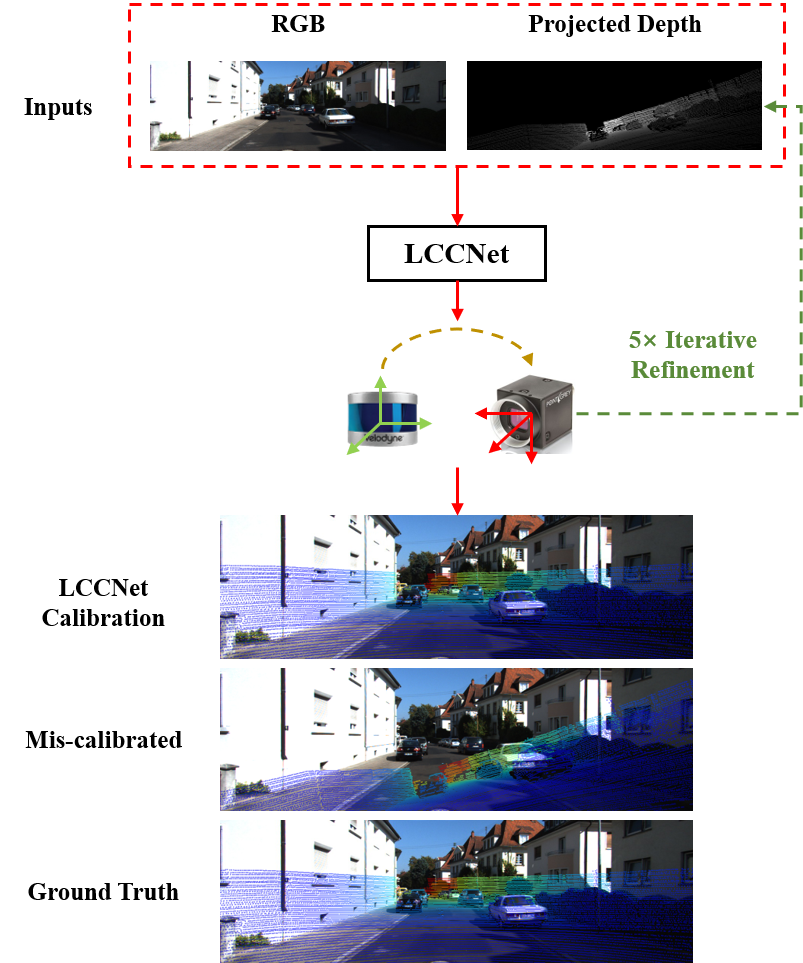
Figure 1: The proposed LCCNet takes the RGB and the projected depth image as inputs to predict the extrinsic parameters between the LiDAR and the camera. The point clouds are re-projected by the predicted extrinsic parameters. The re-projected depth image and the RGB image will be the subsequent inputs of the LCCNet. This process is called iterative refinement. After five times iterative refinements, we obtain the final extrinsic parameters estimation.

1 Introduction

In the past few years, research on autonomous driving technology has developed rapidly. The working environment of autonomous driving is very complex and highly dynamic. No single sensor can ensure stable perception in all scenarios. The fusion of the LiDAR and the camera can provide accurate and stable perception for the surrounding environments or benefit for 3D reconstruction. The basis of LiDAR-camera fusion is the accurate extrinsic calibration, that is, precise estimation of the relative rigid body transformation. LiDAR point cloud and camera image belong to heterogeneous data. Point clouds are sparse 3D data, while images are dense 2D data. Calibration needs to accurately extract the 2D-3D matching correspondences between the pairs of a temporally synchronized camera and LiDAR frames.

Some early calibration works utilized artificial markers, such as checkerboard and specific calibration plates, to calibrate LiDAR and cameras. Most marker-based calibration algorithms are time-consuming, laborious, and offline, not suitable for self-driving car production. During the vehicle’s operation, the position between the sensors will drift slightly with the running time. After a period of operation, the sensors need to be re-calibrated again to eliminate the accumulated error caused by drift. Some current calibration methods for LiDAR and cameras focus on fully automatic and target-less online self-calibration. However, most online self-calibration methods have strict requirements on calibration scenarios, and the calibration accuracy is not as high as offline calibration algorithms based on markers. Some researchers try to apply deep learning to the calibration tasks, using neural networks to predict the 6-DoF rigid body transformation between the two sensors. These methods directly fuse the features extracted from the image and the point cloud without considering the correlation between these two features. e This article proposes a new method for predicting extrinsic calibration parameters of an RGB camera and a LiDAR. More specifically, our contribution can be concluded as follows:

1. LCCNet is a novel end-to-end learning network for LiDAR-Camera extrinsic self-calibration. The network consists of three parts: feature extraction network, feature matching layer, and global feature aggregation network. We use the quaternion as the ground truth during training. Besides the smooth L1-Loss between the predicted calibration and ground truth, an additional point cloud distance loss is presented.

2. The feature matching layer constructs a cost volume that stores the matching costs for RGB features and the corresponding Depth features. To our best knowledge, it is the first deep learning-based LiDAR-camera self-calibration approach that considering the correlation between features of different sensors.

3. To further improve the calibration accuracy, iterative refinement and multiple frames analysis is applied. LCCNet has the best accuracy-speed trade-off compared to other state-of-the-art learning-based calibration methods.

2 Related Work

The calibration between LiDAR and camera can be formulated as a 2D-3D registration problem to obtain the transformation of two sensors’ coordinates. The calibration has three main solutions: (a) Target-based; (b) Target-less; (c) Learning-based.

2.1 Target-based methods

Geige et al. [3] realized LiDAR-camera calibration by multiple printed checkboard patterns on the walls and floors. Define a camera as a reference, all checkerboards in the target image are assigned to the nearest position in the reference image given the expectation. Wang et al. [21] developed a new automatic extrinsic calibration method for 3D LiDAR and panoramic camera using checkerboard. Multiple chessboards or auxiliary calibration object are utilized to provide extra 3D-3D or 2D-3D point correspondences [8, 1].

To obtain more accurate 3D-3D or 2D-3D point correspondences, custom-made markers with a specific appearance, such as polygon plates, hollow circles, unmarked planes, and spherical targets, are introduced for calibration. Park et al. [12] estimated the corresponding 3D points by LiDAR scans on the edges of adjacent polygonal planar boards. The 2D vertical lines detected from the RGB image and the 3D vertical lines estimated from the LiDAR point cloud were regarded as calibration correspondences. [4] employed hollow circles as the calibration target to find the center of the circle in 2D image data and 3D LiDAR point cloud, respectively. Pusztai et al. [13] adopted a carton of known size as the calibration plate to detect the box’s surface. Mishra et al. [10] proposed a LiDAR-camera extrinsic estimation algorithm on unmarked plane target by utilizing Planar Surface Point to Plane and Planar Edge Point to back-projected Plane geometric constraint. The surfaces and contours of the sphere can be accurately detected on point clouds and camera images, respectively. Thus, the spherical targets can achieve fast, and robust extrinsic calibration [9, 19].

2.2 Target-less methods

Tamas et al. [17] proposed a nonlinear explicit correspondence-less calibration method regarding the calibration problem as a 2D-3D registration of a common LiDAR-camera region. Minimal information like depth data and shape of areas are applied to construct the nonlinear registration system, which directly provides the calibration parameters of the LiDAR-camera. Furthermore, [16] advanced a new method of estimating 3D LiDAR and Omnidirectional Cameras’ extrinsic calibration. Without using 2D-3D corresponding points or complex similarity measurement, this method depends on a set of corresponding regions and regresses the pose by solving a small nonlinear system of equations. Pandey et al. [11] adopted the effective correlation coefficient between the surface reflectivity measured by LiDAR and the intensity measured by a camera as one of the extrinsic parameters calibration function, while the other parameters remain unchanged.

Registering the gradient direction of the data obtained by LiDAR and camera was another target-less method. [18] estimated the extrinsic parameter by minimizing the gradient’s misalignment to realize data registration. Kang et al. [6] employed the projection model-based edge alignment to construct the cost function, taking full advantage of the dense photometric and sparse geometry measurements.

2.3 Learning-based methods

RegNet [14] leverages the Convolutional Neural Networks (CNNs) to predict the 6-DoF extrinsic parameters between LiDAR and camera. CalibNet [5] proposed a geometrically supervised deep network capable of automatically estimating the 6-DoF extrinsic parameters in real-time. The end-to-end training is performed by maximizing the geometric and photometric consistency between the input image and the point cloud. RGGNet [22] utilized the Riemannian geometry and deep generative model to build a tolerance-aware loss function.

Semantic information is introduced for obtaining an ideal initial extrinsic parameter. SOIC [20] transforms the initialization problem into the PNP problem of the semantic centroid. In this work, a matching constraint cost function based on the image’s semantic elements and the LiDAR point cloud is presented. By minimizing the cost function, the optimal calibration parameter is obtained. Zhu et al. [23] regard extrinsic calibration as an optimization problem using semantic features to build a novel calibration quality metric.

3 Method

We leverage CNNs to predict the 6-DoF extrinsic calibration between LiDAR and the camera. Our proposed method’s workflow block diagram is shown in Figure 2.

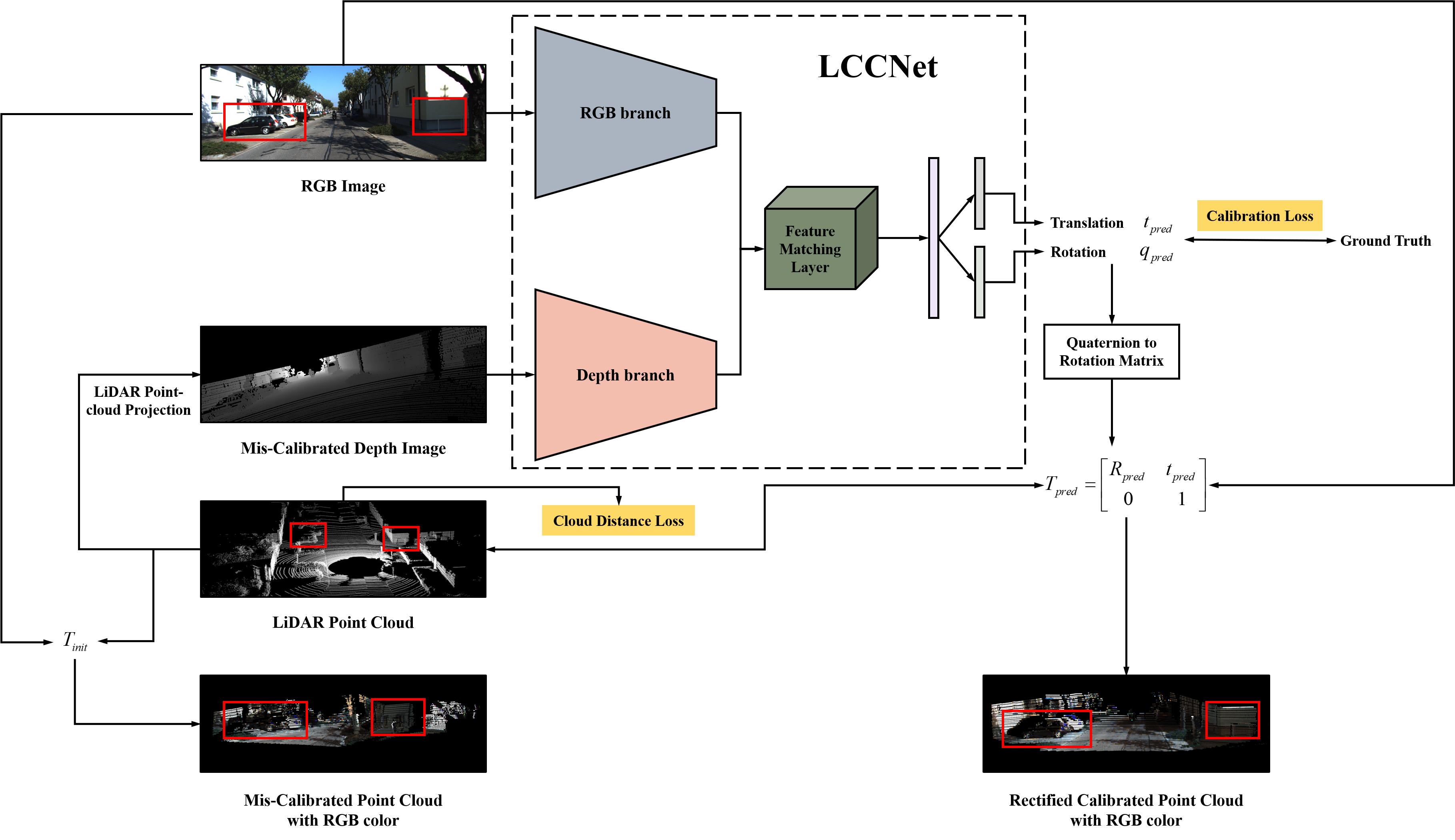
Figure 2: The workflow of our proposed method for the estimation of the extrinsic calibration parameters between 3D LiDAR and 2D camera. The network takes an RGB image from a calibrated camera and a projected sparse depth image from a mis-calibrated LiDAR as input. The output of the network is a 6-DoF rigid-body transformation ${{T}_{pred}}$ that represents the deviation between the initial extrinsic ${{T}_{init}}$ and the ground truth extrinsic ${{T}_{LC}}$. As shown, we notice that the 3D structure highlighted using red rectangles fails to project to their 2D counterparts with the mis-calibrated depth image. When using the predicted transformation ${{T}_{pred}}$ to revise the ${{T}_{init}}$, we can reconstruct a more consistent and accurate 3D scene structure.

3.1 Input Processing

Given initial extrinsic ${{T}_{init}}$ and camera intrinsic $K$, we can generate the depth image by projecting each 3D LiDAR point cloud ${{P}_{i}}=[\begin{matrix}{{X}_{i}}&{{Y}_{i}}&{{Z}_{i}}\end{matrix}]\in{{\mathbb{R}}^{3}}$ from the LiDAR scan onto a virtual image plane with a 2D pixel coordinate ${{p}_{i}}=\left[\begin{matrix}{{u}_{i}}&{{v}_{i}}\end{matrix}\right]\in{{\mathbb{R}}^{2}}$. The projection process is expressed as follows:

$$Z_{i}^{init}\cdot\widehat{{{p}_{i}}} ={Z_{i}^{init}}{{\left[\begin{matrix}{{u}_{i}}&{{v}_{i}}&1\\ \end{matrix}\right]}^{T}}$$ (1)

$$=K\left[{{R}_{init}}|{{t}_{init}}\right]\widehat{{{P}_{i}}}$$

$$=K\left[{{R}_{init}}|{{t}_{init}}\right]{{\left[\begin{matrix}{{X}_{i}}&{{Y}_{i}}&{{Z}_{i}}&1\\ \end{matrix}\right]}^{T}}$$

$${{T}_{init}}=\left[\begin{matrix}{{R}_{init}}&{{t}_{init}}\\ 0&1\\ \end{matrix}\right]$$ (2)

where $\widehat{{{P}_{i}}}$ and $\widehat{{{p}_{i}}}$ represent the homogeneous coordinates of ${{P}_{i}}$ and ${{p}_{i}}$, ${R}_{init}$ and ${t}_{init}$ are the rotation matrix and translation vector of ${T}_{init}$. By using a Z-buffer method, the depth image ${{D}_{init}}$ is computed to determine the visibility of points along the same projection line, where every pixel $({{u}_{i}},{{v}_{i}})$ preserves the depth value $Z_{i}^{init}$ of a 3D point ${{P}_{i}}$ on camera coordinate.

3.2 Network Architecture

The proposed calibration network comprises three parts: feature extraction network, feature matching layer, and feature global aggregation. Since the parameters in each part are differentiable, CNN can be trained end-to-end. We will describe the structure and function of each part of this section.

3.2.1 Feature Extraction Network

The feature extraction network consists of 2 symmetric branches, extracting the RGB image and depth image features. For the RGB branch, we use a pre-trained ResNet-18 network, excluding the full connection layer. The architecture of the depth branch is consistent with the RGB branch. In the depth branch, we switch RELU to Leaky RELU as the activation function.

3.2.2 Feature Matching Layer

After extracting features from two input modalities, a feature matching layer is adopted to calculate the matching cost for associating a pixel in RGB feature maps ${{x}_{rgb}}$ with its corresponding depth feature maps ${{x}_{lidar}}$. Inspired by PWC-Net [15], we take advantage of the correlation layer for feature matching. We define the constructed cost volume as the correlation between ${{x}_{rgb}}$ and ${{x}_{lidar}}$ that stores the matching cost:

$$cv({{p}_{1}},{{p}_{2}})=\frac{1}{N}{{(c({{x}_{rgb}}({{p}_{1}})))}^{T}}c({{x}_{lidar}}({{p}_{2}}))$$ (3)

where $c(x)$ is the flattened vector of feature maps $x$, $N$ is the length of the column vector $c(x)$, $T$is the transpose operator. For the features, we need to compute a local cost volume with a limited range of $d$ pixels, i.e.,${{\left|{{p}_{1}}-{{p}_{2}}\right|}_{\infty}}\leq d$. Since the input feature maps are very small, $1/32$ of the full resolution images, we need to set the value $d$ very small ($d=2$ in this paper). The dimension of the 3D cost volume $cv$ is ${{d}^{2}}\times H\times W$, where $H$ and $W$ donate the height and width of feature maps ${{x}_{rgb}}$ and ${{x}_{lidar}}$, respectively.

3.2.3 Feature Global Aggregation

LCCNet regresses the 6-DoF rigid-body transformation between LiDAR and camera with cost volume features. This network consists of a full connection layer with 512 neurons and two branches with stacked full connection layers representing rotation and translation. The output of the network is a $1\times 3$ translation vector. ${{t}_{pred}}$ and a $1\times 4$ rotation quaternion ${{q}_{pred}}$.

3.3 Loss Function

Given an input pair composed of an RGB image $I$ and a depth image ${{D}_{init}}$, we use two types of loss terms during training: regression loss ${{L}_{T}}$ and point cloud distance loss ${{L}_{P}}$.

$$L={{\lambda}_{T}}{{L}_{T}}+{{\lambda}_{P}}{{L}_{P}}$$ (4)

where ${{\lambda}_{T}}$ and ${{\lambda}_{P}}$ denotes respective loss weight.

3.3.1 Regression Loss

For the translation vector ${{t}_{pred}}$, the smooth $L1$ loss is applied. The derivative of $L1$ loss is not unique at zero, which may affect the convergence of training. Compared to $L1$ loss, the smooth $L1$ loss is much smoother due to the square function’s usage near zero. Regarding the rotation loss ${{L}_{q}}$, since quaternions are essentially directional information, Euclidean distance cannot accurately describe the difference between the two quaternions. Therefore, we use angular distance to represent the difference between quaternions, as defined below:

$${{L}_{R}}={{D}_{a}}({{q}_{gt}},{{q}_{pred}})$$ (5)

where ${{q}_{gt}}$ is the ground truth of quaternion, ${{q}_{pred}}$ is the prediction, ${{D}_{a}}$ is the angular distance of two quaternions [7]. The total regression loss ${{L}_{T}}$ is the combination of translation and rotation loss:

$${{L}_{T}}={{\lambda}_{t}}{{L}_{t}}+{{\lambda}_{q}}{{L}_{R}}$$ (6)

where ${L}_{t}$ is the smooth $L1$ loss for translation, ${{\lambda}_{t}}$ and ${{\lambda}_{q}}$ denotes respective loss weight.

3.3.2 Point Cloud Distance Loss

Besides the regression loss, a point cloud distance constrain is added to the loss function. After transforming the quaternion ${{q}_{pred}}$ to a rotation matrix ${{R}_{pred}}$, we can obtain the homogeneous matrix ${{T}_{pred}}$:

$${{T}_{pred}}=\left[\begin{matrix}{{R}_{pred}}&{{t}_{pred}}\\ 0&1\\ \end{matrix}\right]$$ (7)

Given a group of LiDAR point cloud $P=\left\{{{P}_{1}},{{P}_{2}},\ldots,{{P}_{N}}\right\},{{P}_{i}}\in{{\mathbb{R}}^{3}}$, the point cloud distance loss ${{L}_{P}}$ is defined as:

$${{L}_{p}}=\frac{1}{N}\sum\limits_{i=1}^{N}{{{\left\|T_{LC}^{-1}\cdot T_{pred}^{-1}\cdot{{T}_{init}}\cdot{{P}_{i}}-{{P}_{i}}\right\|}_{2}}}$$ (8)

where ${T}_{LC}$ is the LiDAR-Camera extrinsic matrix, $N$ is the number of point clouds, ${{\left\|\cdot\right\|}_{2}}$ denotes the $L2$ Normalization.

3.4 Calibration Inference and Refinement

The extrinsic calibration parameter between the uncalibrated LiDAR and camera can be obtained by combining the predicted results ${{T}_{pred}}$ of the calibration network and the initial calibration parameter ${{T}_{init}}$. The extrinsic calibration parameter is expressed as:

$${{\widehat{T}}_{LC}}=T_{pred}^{-1}\cdot{{T}_{init}}$$ (9)

In this paper, we train multiple networks on different mis-calibration ranges. We choose the same translation and rotation range as [14]: $\left[-x,x\right],x=\left\{1.5m,1.0m,0.5m,0.2m,0.1m\right\}$, $\left[-y,y\right]$, $y=\left\{20{}^{\circ},10{}^{\circ},5{}^{\circ},2{}^{\circ},1{}^{\circ}\right\}$. The latter smaller range is determined by the maximum mean absolute error (MAE) of the predicted results after training the network using the former larger range. The RGB image and the projected depth map will input the largest range $(\pm 1.5m,\pm 20{}^{\circ})$ network. We regard the prediction ${{T}_{pred}}$ as ${{T}_{0}}$, and re-project the LiDAR point cloud with ${T_{0}^{-1}\cdot{{T}_{init}}}$ to generate a new depth image including more projected LiDAR points. The new depth image and the same RGB image will input to the second range $(\pm 1.0m,\pm 10{}^{\circ})$ network to predict new transformation ${{T}_{1}}$. The aforementioned process is iterated five times to get the final extrinsic calibration matrix.

$${{\widehat{T}}_{LC}}={{\left({{T}_{0}}\cdot{{T}_{1}}\ldots{{T}_{5}}\right)}^{-1}}\cdot{{T}_{init}}$$ (10)

The calibration accuracy can be improved by using the multi-range network iterative refinement. We use the median of the predicted results of multiple frames as the final estimation of the extrinsic parameters.

4 Experiments and Discussion

We evaluate our proposed calibration approach on the KITTI odometry dataset. In this section, we detail the data preprocessing, evaluation metrics, training procedure and discuss the results of different experiments.

4.1 Dataset Preparation

We use the odometry branch of the KITTI dataset [2] to verify our proposed algorithm. KITTI Odometry dataset consists of 21 sequences from different scenarios. The dataset provides calibration parameters between each sensor, among which the calibration parameters between LiDAR and camera were obtained by [3] as the ground truth of extrinsic calibration parameters. In this paper, we only consider the calibration between the LiDAR and the left color camera. Specifically, we used sequences from 01 to 20 for train and validation (39011 frames) and sequence 00 for test (4541 frames). The test dataset is spatially independent of the training dataset, except for a very small subset sequence (about 200 frames), so it can be assumed that the test scenario is not in the training data.

To solve the insufficiency of training data, we add a random deviation $\Delta T$ within a reasonable range to the extrinsic calibration matrix of LiDAR and camera. In this paper, we define the extrinsic parameter ${{T}_{LC}}$ as the Euclidean transformation from the LiDAR coordinate to the camera coordinate. After adding the random parameter $\Delta T$ to ${{T}_{LC}}$, the initial extrinsic ${{T}_{init}}=\Delta T\cdot{{T}_{LC}}$ is obtained. By randomly changing the deviation value, we can acquire a large amount of training data.

4.2 Evaluation Metrics

The experimental results are analyzed according to the rotation and translation of the calibration parameters. The Euclidian distance between the vectors evaluates the translation vector. The absolute error of the translation vector is expressed as follows:

$${{E}_{t}}={{\left\|{{t}_{pred}}-{{t}_{gt}}\right\|}_{2}}$$ (11)

where ${{\left\|\cdot\right\|}_{2}}$ denotes the 2-norm of a vector. We also test the translation vector’s absolute error in $X,Y,Z$ directions, respectively.

Quaternions represent the rotation part. Since quaternion means direction, we use quaternion angle distance to illustrate the difference between quaternions. To test the extrinsic rotation matrix’s angle error on three degrees, we need to transform the rotation matrix to Euler angles and compute the angle error of Roll, Pitch, and Yaw.

4.3 Training Details

During the training stage, we use Adam Optimizer with an initial learning rate $3{{e}^{-4}}$. We train our proposed calibration network on two Nvidia GP100 GPU with batch size 120 and total epochs 120. For the multi-range network, it is not necessary to retrain each network from scratch. Instead, a large-range model can be regarded as the pre-trained model for small-range training to speed up the training process. The model’s training epoch with the largest range is set to 120, while the others are set to 50.

4.4 Results and discussion

The visual results of the multi-range iterations are shown in Figure 3. The final calibration results are shown in Table 1. It is obvious that after multi-range iterations, the calibration error is further reduced and the error distribution is concentrated at a smaller value. Our approach achieves a mean square translation error of 1.588cm, a mean translation error of 0.361cm (x, y, z: 0.243cm, 0.380cm, 0.459cm), and a mean quaternion angle error of $0.163{}^{\circ}$, a mean angle error of $0.030{}^{\circ}$(roll, pitch, yaw: $0.030{}^{\circ},\text{ }0.019{}^{\circ},\text{ }0.040{}^{\circ}$).

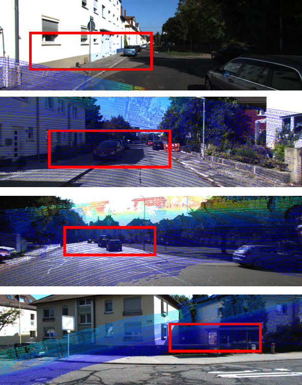
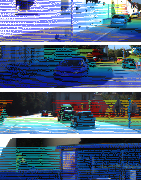
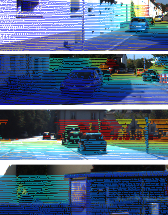
Figure 3: Results of different single-shot calibration after multi-range iteration on the test dataset. (a) Initial Calibration, (b) Ground truth, (c) Calibration results.

Table 1: The results of the multi-range network iteration

Results of multi-range		Translation (cm)				Rotation (∘)
		${{E}_{t}}$	X	Y	Z	${{E}_{R}}$	Roll	Pitch	Yaw
After $20{}^{\circ}/1.5\operatorname{m}$ network	Mean	17.834	11.849	5.169	7.613	1.235	0.170	0.676	0.594
	Median	13.423	14.415	5.337	4.188	0.898	0.033	0.615	0.549
	Std.	17.165	5.783	3.847	6.492	1.427	0.260	0.580	0.216
After $10{}^{\circ}/1.0\operatorname{m}$ network	Mean	6.291	2.045	4.195	2.238	0.594	0.378	0.391	0.405
	Median	5.662	1.929	3.066	2.437	0.452	0.271	0.156	0.218
	Std.	3.494	1.629	3.673	1.683	0.637	0.422	0.480	0.453
After $5{}^{\circ}/0.5\operatorname{m}$ network	Mean	3.915	1.267	2.212	1.107	0.414	0.309	0.330	0.334
	Median	3.712	1.390	2.410	1.057	0.297	0.028	0.026	0.071
	Std.	0.809	0.686	0.989	0.570	0.541	0.507	0.538	0.479
After $2{}^{\circ}/0.2\operatorname{m}$ network	Mean	2.069	0.664	0.633	0.281	0.288	0.132	0.103	0.081
	Median	1.592	0.475	0.455	0.316	0.215	0.038	0.040	0.045
	Std.	1.859	0.497	0.581	0.112	0.465	0.196	0.140	0.099
After $1{}^{\circ}/0.1\operatorname{m}$ network	Mean	1.588	0.243	0.380	0.459	0.163	0.030	0.019	0.040
	Median	1.011	0.262	0.358	0.352	0.121	0.030	0.001	0.022
	Std.	1.776	0.053	0.253	0.254	0.435	0.019	0.031	0.039

From Figure 4, we can find that our proposed calibration method can accurately predict the extrinsic calibration parameters for different random initial parameters. Although there is a great difference between the two initial parameters shown in Figure 4(a), their corresponding calibration results are almost in full accord. Figure 4(c) also shows that the two tests’ error distributions are very similar. The proposed method has a high tolerance for the deviation of initial extrinsic parameters; that is, the algorithm can perform the calibration task accurately even a few point clouds are projected into the image. The results of the multiple frames analysis are exhibited in Table 2, the algorithm achieves a mean square translation error of 1.010cm, a mean translation error of 0.297cm (x, y, z: 0.262cm, 0.271cm, 0.357cm) and a mean quaternion angle error of $0.122{}^{\circ}$, a mean angle error of $0.017{}^{\circ}$(roll, pitch, yaw: $0.020{}^{\circ},\text{ }0.012{}^{\circ},\text{ }0.019{}^{\circ}$). The comparison results with other learning-based extrinsic calibration methods in Table 3 express that our proposed method is superior to these state-of-the-art algorithms. Due to most of the training datasets are the same, we do not re-train the baselines.

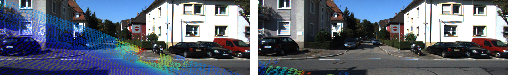
(a) Initial calibration

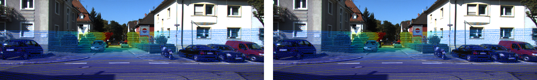
(b) Calibration results

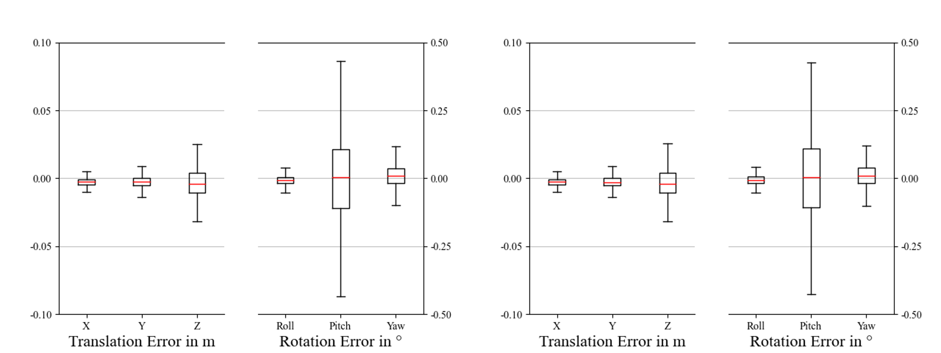
(c) Calibration error with temporal filtering

Figure 4: Examples of the error distribution for a miscalibration, which is fixed over the test sequence. Five networks are executed iteratively ($20{}^{\circ}/1.5m,10{}^{\circ}/1.0m,5{}^{\circ}/0.5m,2{}^{\circ}/0.2m,1{}^{\circ}/0.1m$).

Table 2: The results of the calibration error with multiple frames analysis

Results	Translation (cm)				Rotation (∘)
	${{E}_{t}}$	X	Y	Z	${{E}_{R}}$	Roll	Pitch	Yaw
Mean	1.010	0.262	0.271	0.357	0.122	0.020	0.012	0.019
Median	1.010	0.260	0.274	0.337	0.122	0.020	0.010	0.019
Std.	0.007	0.087	0.109	0.148	0.001	0.008	0.007	0.009

Table 3: Comparison results with other learning-based calibration algorithms.

Method	Mis-calibrated range	Translation absolute Error (cm)				Rotation absolute Error (∘)
		mean	X	Y	Z	mean	Roll	Pitch	Yaw
Regnet [14]	$[-1.5m,1.5m]/[-20{}^{\circ},20{}^{\circ}]$	6	7	7	4	0.28	0.24	0.25	0.36
Calibnet [5]	$[-0.2m,0.2m]/[-10{}^{\circ},10{}^{\circ}]$	4.34	4.2	1.6	7.22	0.41	0.18	0.9	0.15
Ours	$[-1.5m,1.5m]/[-20{}^{\circ},20{}^{\circ}]$	0.297	0.262	0.271	0.357	0.017	0.020	0.012	0.019

5 Conclusion

We propose a novel learning-based extrinsic calibration method for the 3D LiDAR and the 2D camera. The calibration network consists of three parts: feature extraction network, feature matching layer and feature global aggregation network. We construct a cost volume between the RGB features and the depth features for feature matching instead of concatenating them directly compared to other learning-based approaches. To deal with the training data’s insufficiency, we add a random deviation to the extrinsic transformation matrix. Therefore, the network does not predict the extrinsic parameters between LiDAR and camera directly, but the random deviation. Besides the extrinsic ground truth’s supervision, we also add a point cloud constrain to the loss function. Iteratively refinement with multi-range networks and multiple frames analysis will further decrease the calibration error. Our method achieves a mean absolute calibration error of $0.297cm$ in translation and $0.017{}^{\circ}$ in rotation with miscalibration magnitudes of up to $\pm 1.5m$ and $\pm 20{}^{\circ}$, which is superior to other state-of-the-art learning-based methods.

References

- [1] Pei An, Tao Ma, Kun Yu, Bin Fang, Jun Zhang, Wenxing Fu, and Jie Ma. Geometric calibration for lidar-camera system fusing 3d-2d and 3d-3d point correspondences. Optics express, 28(2):2122–2141, 2020.
- [2] Andreas Geiger, Philip Lenz, and Raquel Urtasun. Are we ready for autonomous driving? the kitti vision benchmark suite. In IEEE Conf. Comput. Vis. Pattern Recog., pages 3354–3361. IEEE, 2012.
- [3] Andreas Geiger, Frank Moosmann, Ömer Car, and Bernhard Schuster. Automatic camera and range sensor calibration using a single shot. In 2012 IEEE International Conference on Robotics and Automation (ICRA), pages 3936–3943. IEEE, 2012.
- [4] Carlos Guindel, Jorge Beltrán, David Martín, and Fernando García. Automatic extrinsic calibration for lidar-stereo vehicle sensor setups. In 2017 IEEE 20th international conference on intelligent transportation systems (ITSC), pages 1–6. IEEE, 2017.
- [5] Ganesh Iyer, R Karnik Ram, J Krishna Murthy, and K Madhava Krishna. Calibnet: Geometrically supervised extrinsic calibration using 3d spatial transformer networks. In 2018 IEEE/RSJ International Conference on Intelligent Robots and Systems (IROS), pages 1110–1117. IEEE, 2018.
- [6] Jaehyeon Kang and Nakju L Doh. Automatic targetless camera–lidar calibration by aligning edge with gaussian mixture model. Journal of Field Robotics, 37(1):158–179, 2020.
- [7] Alex Kendall, Matthew Grimes, and Roberto Cipolla. Posenet: A convolutional network for real-time 6-dof camera relocalization. In Int. Conf. Comput. Vis., pages 2938–2946, 2015.
- [8] Eung-su Kim and Soon-Yong Park. Extrinsic calibration between camera and lidar sensors by matching multiple 3d planes. Sensors, 20(1):52, 2020.
- [9] Julius Kümmerle, Tilman Kühner, and Martin Lauer. Automatic calibration of multiple cameras and depth sensors with a spherical target. In 2018 IEEE/RSJ International Conference on Intelligent Robots and Systems (IROS), pages 1–8. IEEE, 2018.
- [10] Subodh Mishra, Gaurav Pandey, and Srikanth Saripalli. Extrinsic calibration of a 3d-lidar and a camera. In 2020 IEEE Intelligent Vehicles Symposium (IV), pages 1765–1770, 2020.
- [11] Gaurav Pandey, James R McBride, Silvio Savarese, and Ryan M Eustice. Automatic extrinsic calibration of vision and lidar by maximizing mutual information. Journal of Field Robotics, 32(5):696–722, 2015.
- [12] Yoonsu Park, Seokmin Yun, Chee Sun Won, Kyungeun Cho, Kyhyun Um, and Sungdae Sim. Calibration between color camera and 3d lidar instruments with a polygonal planar board. Sensors, 14(3):5333–5353, 2014.
- [13] Zoltan Pusztai and Levente Hajder. Accurate calibration of lidar-camera systems using ordinary boxes. In Int. Conf. Comput. Vis., pages 394–402, 2017.
- [14] Nick Schneider, Florian Piewak, Christoph Stiller, and Uwe Franke. Regnet: Multimodal sensor registration using deep neural networks. In 2017 IEEE intelligent vehicles symposium (IV), pages 1803–1810. IEEE, 2017.
- [15] Deqing Sun, Xiaodong Yang, Ming-Yu Liu, and Jan Kautz. Pwc-net: Cnns for optical flow using pyramid, warping, and cost volume. In IEEE Conf. Comput. Vis. Pattern Recog., pages 8934–8943, 2018.
- [16] Levente Tamas, Robert Frohlich, and Zoltan Kato. Relative pose estimation and fusion of omnidirectional and lidar cameras. In Eur. Conf. Comput. Vis., pages 640–651. Springer, 2014.
- [17] Levente Tamas and Zoltan Kato. Targetless calibration of a lidar-perspective camera pair. In Int. Conf. Comput. Vis., pages 668–675, 2013.
- [18] Zachary Taylor, Juan Nieto, and David Johnson. Multi-modal sensor calibration using a gradient orientation measure. Journal of Field Robotics, 32(5):675–695, 2015.
- [19] Tekla Tóth, Zoltán Pusztai, and Levente Hajder. Automatic lidar-camera calibration of extrinsic parameters using a spherical target. In 2020 IEEE International Conference on Robotics and Automation (ICRA), pages 8580–8586. IEEE, 2020.
- [20] Weimin Wang, Shohei Nobuhara, Ryosuke Nakamura, and Ken Sakurada. Soic: Semantic online initialization and calibration for lidar and camera. arXiv preprint arXiv:2003.04260, 2020.
- [21] Weimin Wang, Ken Sakurada, and Nobuo Kawaguchi. Reflectance intensity assisted automatic and accurate extrinsic calibration of 3d lidar and panoramic camera using a printed chessboard. Remote Sensing, 9(8):851, 2017.
- [22] Kaiwen Yuan, Zhenyu Guo, and Z Jane Wang. Rggnet: Tolerance aware lidar-camera online calibration with geometric deep learning and generative model. IEEE Robotics and Automation Letters, 5(4):6956–6963, 2020.
- [23] Yufeng Zhu, Chenghui Li, and Yubo Zhang. Online camera-lidar calibration with sensor semantic information. In 2020 IEEE International Conference on Robotics and Automation (ICRA), pages 4970–4976. IEEE, 2020.