Coarse to Fine: Multi-label Image Classification with Global/Local Attention

Abstract

In our daily life, the scenes around us are always with multiple labels especially in a smart city, i.e., recognizing the information of city operation to response and control. Great efforts have been made by using Deep Neural Networks to recognize multi-label images. Since multi-label image classification is very complicated, people seek to use the attention mechanism to guide the classification process. However, conventional attention-based methods always analyzed images directly and aggressively. It is difficult for them to well understand complicated scenes. In this paper, we propose a global/local attention method that can recognize an image from coarse to fine by mimicking how human-beings observe images. Specifically, our global/local attention method first concentrates on the whole image, and then focuses on local specific objects in the image. We also propose a joint max-margin objective function, which enforces that the minimum score of positive labels should be larger than the maximum score of negative labels horizontally and vertically. This function can further improve our multi-label image classification method. We evaluate the effectiveness of our method on two popular multi-label image datasets (i.e., Pascal VOC and MS-COCO). Our experimental results show that our method outperforms state-of-the-art methods.

I Introduction

In a smart city[1, 2], multi-label scenes are much common, and accurately recognizing multiple label is quite important. For example, by recognizing every traffic routes and analyzing flows through monitors, a smart city is able to ease traffic jams. Recently, some study about multi-label image classification in smart cities are draw attention of researchers[3, 4]. Multi-label image classification seeks to recognize all possible objects/labels in a given image. Because of the dramatic development of deep learning and the availability of large-scale datasets such as ImageNet [5], there exist many studies on single-label image classification [6, 7]. However, scenes around us are always with multiple objects/labels. Unfortunately, multi-label image classification are more difficult than single-label one since the complicated structure and the internal label dependencies.

Recently, methods based on Deep Neural Networks become popular. On the one hand, due to the success of Convolutional Neural Networks (CNNs) on single-label image classification, a large number of methods directly apply CNNs to multi-label tasks[8, 9, 10, 11]. On the other hand, some researchers additionally leverage Recurrent Neural Networks (RNNs) to model the dependencies among labels [12, 13, 14]. However, all the aforementioned works consider to indiscriminately analyze the whole image when building a multi-label image classification model, so that useless and redundant information would be equally taken into account. For example, some blank or blur backgrounds may be behind key objects in an image are equally used in the model learning process.

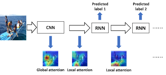
In this paper, inspired by the success of the attention mechanism [15, 16, 17, 18],we propose a global/local attention method to for multi-label image classification that can classify images from coarse to fine. The model can imitate how human beings observe a scenery image—they first observes the image with a global attention to find the areas that may have objects, and then focuses on these areas to consider what object is inside each area. The process is simply shown in Fig. 1. The global attention, which is generated from the final convolutional layer in CNN, denotes a general attentive area, i.e., an overview of an image. Then, we generate local attention in every step of RNN, which denotes each specific attentive area for each predicted label. Additionally, we propose a joint max-margin objective function to separate the positive and negative prediction in the time domain, which can effectively improve the performance. We evaluate our method on two popular multi-label image datasets, and the experimental results show that our method is better than the other state-of-the arts.

Figure 1: The schematic of the proposed architecture. The encoder CNN extracts feature from images, and computes the global attention from the feature map. Then, the attended features are sent to the decoder RNN. At every step of RNN, we focus on each local attention to guide the prediction.

II Related Work

II-A Multi-label image classification

Multi-label classification is with wide applications in many areas, especially for image classification, and lots of efforts have been made for this task. Traditional methods can be decomposed into two categories [19], i.e.the problem transformation [20, 21, 22] and algorithm adaptation [23, 24]. Recently, methods based on CNNs become popular in single-label image classification for its strong capability in learning discriminative features. Some researchers attempted to directly apply CNNs on multi-label image classification. Gong et al.  [8] built a CNN architecture similar to [9] to tackle this problem, and trained a CNN model with top-k ranking objectives. Wei et al.  [11] fine-tuned the network pre-trained on ImageNet [5] with the squared loss for multi-label image classification (I-FT). Some works employed an object detection framework to strengthen the performance of CNNs. For example, Wei et al.  provided a regional solution that allows predicting labels independently at the regional level (H-FT). Some approaches use RNNs to model label dependencies. Wang et al.  [12] utilized CNNs to extract image features, and then utilized RNNs to model correlations among labels. In [12], the authors combined the image embedding with the output of Long Short-Term Memory (LSTM) every step, and then passed the combined vector to the final fully connected layer to predict the current label. Liu et al.  [14] regularized CNN by ground truth semantic concepts, and then used the prediction to set the LSTM initial states. Although the performance of multi-label classification has been significantly improved by using CNNs and RNNs, these methods always consider to extract features from the whole image. This results in that much redundant information would be equally considered in the multi-label classification model training process. In fact, relevant objects may be only little parts of an image. Some researchers started to leverage the attention mechanism to guide multi-label classification.

II-B Attention mechanism

The attention mechanism forces a learning model to focus on relevant parts of an original data. Bahdanau et al.  [15] proposed a model to search a set of possible positions while generating the target word in Neural Machine Translation. This mechanism was then applied to the research field that combines vision and language. In [16], Xu et al.  took hard and soft attention-based methods to generate image descriptions. You et al.  [18] ran a set of attribute detectors to get a list of visual attributes and fuse them into the RNN hidden state. Lu et al.  [25] proposed a co-attention model that combines the language information and the image information in the task of Visual Question Answering. With the attention mechanism, the model can learn the attention by itself, which can intuitively guide the model to observe the data. However, few works applied this mechanism to the multi-label image classification. Zhu et al.  [26] proposed to learn semantic and spatial relations jointly and generate attention maps for all labels. Although their work computed attentions for all labels, this may also result in a large number of additional parameters.

In this paper, we argue that the attention can also be learned from coarse to fine. Almost all existing attention-based methods analyzed the whole image directly and cursorily, and we think this should follow a progress. When coming across a complicated scene, we need to look around in general firstly and then search specific objects one by one. Therefore, we propose a global-local attention method for multi-label image classification. The details of our proposed method will be explained in Section III.

III Method

III-A Problem definition

Multi-label classification is to predict all possible labels for an image. Given a set of images $\mathcal{X}=\{\bm{x}_{1},\bm{x}_{2},\dots,\bm{x}_{N}\}$ and their corresponding labels $\mathcal{Y}=\{\bm{y}_{1},\bm{y}_{2},\dots,\bm{y}_{N}\}$, where $N$ is the number of images in the set, our work is to learn a hypothesis $h:\mathcal{X}\rightarrow\mathcal{Y}$ that maps an input image $\bm{x}$ to output $\bm{y}$. For the i-th image $\bm{x}_{i}$, we denote the corresponding labels as $\bm{y}_{i}=\{y_{i1},y_{i2},\dots,y_{iC}\}$, where $y_{ij}=1$ means the image $\bm{x}_{i}$ is labeled with label $j$ while $y_{ij}=0$ is on the contrary. $C$ is the number of possible labels.

III-B The framework of our model

Our overall model follows the encoder-decoder design pattern [27], which transforms data from one representation to another. In the proposed model, the encoder is a VGG-16 model [6], which has been proved to extract features from image effectively. From the VGG-16 model, we extract two types of features from each image. The first type of features comes from the final convolutional layer, presenting the structural information of an image and denoting as $\bm{f}_{conv}=\{\bm{a}_{1},\bm{a}_{2},\dots,\bm{a}_{L}\}$, where $L$ is the number of regions in the feature map. The other type of features is from the last fully-connected layer, including more higher-level information of an image and denoting as $\bm{f}_{fc}$. The decoder is an RNN model. In this paper, we used Long Short-Term Memory [28] (LSTM). LSTM adds three extra gates to the vanilla RNN, i.e., the input gate, the forget gate and the output gate. Following [12], multiple labels in multi-label classification can be regarded as a sequence, and the RNN decoder is used to recognize each specific object one by one.

III-C Visual attention mechanism

In this section, we describe our visual attention mechanism. In our model, we leverage two types of attentions, i.e., the global attention and the local attention. For the global attention, a more general attentive area is highlighted, while a more fine-grained one is highlighted for local attention.

III-C1 Global attention

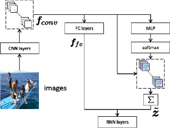
Our global attention $\hat{\bm{\alpha}}=\{\hat{\alpha}_{1},\hat{\alpha}_{2},\dots,\hat{\alpha}_{N}\}$ is computed from $\bm{f}_{conv}$. For the $i$-th region, it corresponds to a positive weight

(a) Global attention

(b) Local attention

Figure 2: The architecture to obtain global and local attention.

$$\hat{\alpha}_{i}=\text{softmax}(\tanh(\bm{W}_{g}\bm{a}_{i}+\bm{b}_{g})),$$ (1)

where $\hat{\alpha}_{i}$ is a scalar presenting the degree of the $i$-th region’s importance. With $\hat{\bm{\alpha}}$, we can compute the excepted aligned global context $\hat{\bm{z}}$, and the process can be shown in Fig. 2(a).

$$\hat{\bm{z}}=\sum_{i=1}^{N}\hat{\alpha}_{i}\bm{a}_{i}.$$ (2)

Note that we used the sum of all weighted $\bm{a}_{i}$ to compute the expected aligned contexts. This attentive context shows how the weight influences the feature maps.Thus, unlike traditional sequence learning that zero-initializing LSTM, in our architecture, we initialized it with the average of $\hat{\bm{z}}$.

$$\bm{c}_{0}=I_{c}(\hat{\bm{z}}/L),~{}\bm{h}_{0}=I_{h}(\hat{\bm{z}}/L),$$ (3)

The initialization of parameters is quite important. [29] considered that the attention mechanism lacks global modeling abilities in common sequential learning. Initializing the memory cell and the hidden state in this way helps LSTM learn the whole non-attentive feature maps and a glance to the original image. Moreover, because $\hat{\bm{z}}$ is an attentive global context, our model can first give a general area that may contain some meaningful objects.

III-C2 Local attention

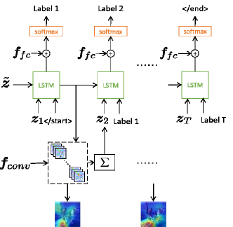
After the proposed model has observed an image in a general way, we expect our model like human beings to focus on every specific object. Therefore, as shown in Fig. 2(b), our model computes local attention at each step of LSTM.

For all regions at step $t$, similar to the global attention, we used a positive weight $\bm{\beta}_{t}=\{\beta_{t1},\beta_{t2},\dots,\beta_{tN}\}$ to decide which location is the right attentive place for the next label. Its element $\beta_{ti}$ is computed by

$$\beta_{ti}=\text{softmax}({g(\bm{a}_{i},\bm{h}_{t-1})}).$$ (4)

In Eq. (4), $\beta_{ti}$ presents the prior hidden state $\bm{h}_{t-1}$, $g$ is a simple Multi-Layer Perceptron, which reflects the importance of the feature $\bm{a}_{i}$ as well as the hidden state $\bm{h}_{t-1}$ and decides the next state of LSTM. Therefore, LSTM is forced to pay more attention to these regions with larger weights. Then, we can compute the dynamic context $\bm{z}_{t}$ as follows.

$$\bm{z}_{t}=\beta_{t}\cdot\phi(\{\bm{a}_{i}\},\bm{\alpha}_{t})=\beta_{t}\sum_{i=1}^{N}\alpha_{ti}\bm{a}_{i}.$$ (5)

We treated their set $\bm{z}_{t}$ as another special features and feeded them into LSTM as the next input. That means for every step of the LSTM’s recurrence, the model must take the possible area into account and overlook some unimportant information. As a consequence, following [30], the forward passing at step $t$ can be defined as follows.

$$\bm{g}_{t} =\tanh(\bm{W}_{xc}\bm{y}_{t}+\bm{W}_{hc}\bm{h}_{t-1}+\bm{W}_{zc}\bm{z}_{t}+\bm{b}_{c}),$$ (6)

$$\bm{i}_{t} =\sigma(\bm{W}_{xi}\bm{y}_{t}+\bm{W}_{hi}\bm{h}_{t-1}+\bm{W}_{zi}\bm{z}_{t}+\bm{b}_{i}),$$ (7)

$$\bm{f}_{t} =\sigma(\bm{W}_{xf}\bm{y}_{t}+\bm{W}_{hf}\bm{h}_{t-1}+\bm{W}_{zf}\bm{z}_{t}+\bm{b}_{f}),$$ (8)

$$\bm{o}_{t} =\sigma(\bm{W}_{xo}\bm{y}_{t}+\bm{W}_{ho}\bm{h}_{t-1}+\bm{W}_{zo}\bm{z}_{t}+\bm{b}_{o}),$$ (9)

$$\bm{c}_{t} =\bm{f}_{t}\odot\bm{c}_{t-1}+\bm{i}_{t}\odot\bm{g}_{t},$$ (10)

$$\bm{h}_{t} =\bm{o}_{t}\odot\tanh(\bm{c}_{t}),$$ (11)

where all $\bm{W}$-s and $\bm{b}$-s are trainable weights and biases. $\bm{y}_{t}$ denotes the input label in step $t$, and $\bm{h}_{t-1}$ is the last hidden state.

III-D Objective function

III-D1 Horizontal max-margin objective

We obtained a prediction at every step for the $i$-th image. Therefore, we will obtain a set of predictions $\bm{P}_{i}=\{\bm{p}_{i1},\bm{p}_{i2},\dots,\bm{p}_{iT}\}$ at the end of the sequence. For the prediction at the $t$-th step $\bm{p}_{it}$, it is a vector with length $L$, where $L$ is the number of all classes. Actually, we obtained the final prediction $\hat{\bm{p}}_{i}=\{p_{i}^{j},p_{i}^{j},\dots,p_{i}^{j}\}$ by a max-pooling for each class. For the $j$-th class, we have

$$p_{i}^{j}=\text{max}(p_{i1}^{j},p_{i2}^{j},\dots,p_{iT}^{j}).$$ (12)

To separate the positive and negative prediction, we assumed that a max margin is between the minimum positive and maximum negative prediction. That is,

$$\text{min}_{+}(\hat{\bm{p}}_{i})>\text{max}_{-}(\hat{\bm{p}}_{i})+\epsilon$$ (13)

where $\text{min}_{+}(\hat{\bm{p}}_{i})$ and $\text{max}_{-}(\hat{\bm{p}}_{i})$ mean the minimum positive and the maximum negative prediction respectively. $\epsilon$ is the joint max-margin, and is pre-defined before training. As a result, we have a constrain for the prediction as follows.

$$R_{1}=\sum_{i=1}^{N}\text{max}(\text{min}_{+}(\hat{\bm{p}}_{i})-\text{max}_{-}(\hat{\bm{p}}_{i})+\epsilon,0)$$ (14)

TABLE I: Experimental Results on Pascal VOC 2007.

	plane	bike	bird	boat	bottle	bus	car	cat	chair	cow	table	dog	horse	motor	person	plant	sheep	sofa	train	tv	mAP
INRIA	77.2	69.3	56.2	66.6	45.5	68.1	83.4	53.6	58.3	51.1	62.2	45.2	78.4	69.7	86.1	52.4	54.4	54.3	75.8	62.1	63.5
FV	75.7	64.8	52.8	70.6	30.0	64.1	77.5	55.5	55.6	41.8	56.3	41.7	76.3	64.4	82.7	28.3	39.7	56.6	79.7	51.5	58.3
CNN-SVM	88.5	81.0	83.5	82.0	42.0	72.5	85.3	81.6	59.9	58.5	66.5	77.8	81.8	78.8	90.2	54.8	71.1	62.6	87.4	71.8	73.9
I-FT	91.4	84.7	87.5	81.8	40.2	73.0	86.4	84.8	51.8	63.9	67.9	82.7	84.0	76.9	90.4	51.5	79.9	54.3	89.5	65.8	74.5
HCP-1000C	95.1	90.1	92.8	89.9	51.5	80.0	91.7	91.6	57.7	77.8	70.9	89.3	89.3	85.2	93.0	64.0	85.7	62.7	94.4	78.3	81.5
HCP-2000C	96.0	92.1	93.7	93.4	58.7	84.0	93.4	92.0	62.8	89.1	76.3	91.4	95.0	87.8	93.1	69.9	90.3	68.0	96.8	80.6	85.2
CNN-RNN	96.7	83.1	94.2	92.8	61.2	82.1	89.1	94.2	64.2	83.6	70.0	92.4	91.7	84.2	93.7	59.8	93.2	75.3	99.7	78.6	84.0
VGG	96.5	89.5	92.8	92.8	58.0	85.6	90.0	92.5	70.3	85.2	76.0	91.7	89.9	87.0	94.3	68.8	87.1	68.3	97.3	80.7	84.7
VGG+LSTM	96.7	91.1	93.8	92.7	55.4	81.7	90.2	91.0	67.6	83.9	75.4	91.7	94.3	90.8	94.8	65.5	86.6	67.5	97.1	79.4	84.4
VGG+LSTM+L	97.0	92.5	93.8	93.3	59.3	82.6	90.6	92.0	73.4	82.4	76.6	92.4	94.2	91.4	95.3	67.9	88.6	70.1	96.8	81.5	85.2
VGG+LSTM+L/G	97.5	91.0	94.2	95.0	56.2	84.9	90.9	92.3	71.6	86.8	76.2	92.0	94.6	89.5	95.5	66.4	86.2	70.0	96.9	81.4	85.4
VGG+LSTM+L/G+MM	97.0	92.4	94.4	93.6	59.1	83.8	90.7	92.5	69.8	84.2	76.9	91.8	95.1	91.1	96.2	66.2	88.0	69.2	96.2	82.6	85.6

Figure 3: Visualization of the attentive images on PASCAL VOC 2007.

Figure 4: Visualization of attentive images on PASCAL VOC 2007 for every 10 epochs.

TABLE II: Experimental Results on MS-COCO.

Method	P@3/5(%)$\uparrow$	R@3/5(%)$\uparrow$	F@3/5(%)$\uparrow$	H@3/5$\downarrow$	A@3/5(%)$\uparrow$	1-err(%)$\downarrow$	C$\downarrow$	rloss$\downarrow$	mAP(%)$\uparrow$
CNN [12]	-/-	-/-	-/-	-/-	-/-	-	-	-	57.20
CNN-RNN [12]	-/-	-/-	-/-	-/-	-/-	-	-	-	61.20
VGG	58.78/42.23	71.96/81.14	64.70/55.55	0.029/0.046	46.25/36.98	11.25	49.31	0.032	63.94
VGG+LSTM	57.92/41.18	70.87/79.24	63.74/54.19	0.030/0.047	45.32/35.79	12.12	47.81	0.050	61.54
VGG+LSTM+L	58.76/42.55	71.67/81.45	64.58/55.90	0.029/0.045	46.19/37.33	12.33	49.80	0.031	63.93
VGG+LSTM+L/G	58.98/42.62	71.86/81.43	64.79/55.95	0.029/0.045	46.40/37.52	11.88	49.83	0.029	64.07
VGG+LSTM+L/G+MM	59.08/42.72	71.95/81.67	64.88/56.10	0.029/0.045	46.46/37.39	11.61	49.63	0.031	64.64

III-D2 Vertical max-margin objective

With only the horizontal max-margin objective, the distance between positive and negative labels will be larger. However, for each step, we only expect to predict one label. Thus, even if the label is not predicted, the margin still exists. Therefore, we proposed another vertical max-margin objective. The prediction list $\bm{P}_{i}=\{\bm{p}_{i1},\bm{p}_{i2},\dots,\bm{p}_{iT}\}$ can be regarded as a matrix $\bm{Q}\in\mathbb{R}^{T\times L}$, and $\bm{Q}_{i}=[\bm{p}_{i1},\bm{p}_{i2},\dots,\bm{p}_{iT}]^{\top}$, where the $t$-th row presents the prediction in step $t$ and the $l$-th column presents the $l$-th class. Thus, for each class the minimum positive and maximum negative also have a max margin.

$$\text{min}_{+}(\bm{Q}_{i,j})>\text{max}_{-}(\bm{Q}_{i,j})+\epsilon_{v},~{}~{}j\in{1,2,\dots,L}.$$ (15)

where $\text{min}_{+}(\bm{Q}_{i,j})$ means the minimum positive prediction on class $j$ for each step, and $\text{max}_{-}(\bm{Q}_{i,j})$ means the maximum negative prediction. The constrain in the vertical direction can be denoted as

$$R_{2}=\sum_{i=1}^{N}\text{max}(\text{min}_{+}(\bm{Q}_{i,j})-\text{max}_{-}(\bm{Q}_{i,j})+\epsilon_{v},0)$$ (16)

III-D3 Final objective

Although we do prediction at every step of RNN, we defined the final prediction as the max-pooling of the prediction of each step. Formally, given a training sample $\{\bm{x}_{i},\bm{y}_{i}\}$, we expect the model to give the prediction $\hat{\bm{y}_{i}}$.

We construct the final objective function as

$$\mathcal{L}(\mathcal{X},\mathcal{Y})$$ (17)

$$= -\frac{1}{N}\sum_{i=1}^{N}\sum_{j=1}^{C}[y_{ij}\log(\hat{y}_{ij})+(1-y_{ij})\log(1-\hat{y}_{ij})]$$

$$+\lambda_{1}R_{1}+\lambda_{2}R_{2},$$

where $\lambda_{1}$ and $\lambda_{2}$ are the regular parameters.

IV Experiments

IV-A Datasets and Experimental Settings

We used two popular multi-label image datasets, i.e., The PASCAL Visual Object Classes Challenge (Pascal VOC) [31] and Microsoft COCO (MS-COCO) [32], to evaluate our method. Pascal VOC 2007 has 5,011 training examples and 4,952 testing examples of 20 classes. MS-COCO dataset [32] has 123,287 images (82,783 training and 40,504 validating examples) of 80 different classes.

For the proposed method, we used VGG-16 [6] as our back-bone model of the encoder CNN. The ${\bm{f}}_{conv}$ are extracted from the last convolutional layer conv5_3 and ${\bm{f}}_{fc}$ are extracted from the last fully-connected layer fc_7. The parameters of VGG-16 are pre-trained on ImageNet. We set $\lambda_{1}=5\times 10^{-2}$ and $\lambda_{2}=5\times 10^{-2}$ to determine the importance of the max-margin regular term. In our experimental results, we used “L” and “G” to represent the model with local attention and/or global attention respectively. And we used “MM” to represent the model with joint max-margin objective. We used the several common metrics (Precision[P], Recall[R], F1-Score[F], Hamming loss[H], Accuracy[A], One error[1-err], Coverage[C], Rank loss[rloss], Mean average precision[mAP]) to evaluate our method and comparison methods, and X@$k$ means metric X on top $k$. $\downarrow$ means the lower the metric, the better the performance is, while $\uparrow$ is on the contrary.

IV-B Performance on Pascal VOC

We first evaluated our method on Pascal VOC 2007. The comparison to the state-of-the-art methods is shown in Table I. Comparison methods include the follows:

• INRIA [33] combines object localization and image classification efficiently and makes both improved.

• FV [34] applies Fisher Kernel [35] to multi-label image classification.

• CNN-SVM uses CNN to extract the feature of images and classifies images with SVM [36, 37, 38].

• IFT trains an AlexNet with a softmax loss.

• [11], based on IFT, fine-tunes the network with multiple hypotheses, and augments 1000/2000 additional classes.

• CNN-RNN [12] uses a CNN as an encoder and a RNN as a decoder, and predicts labels sequentially.

From Table I, We can see that our method outperforms these state-of-the-arts. First, our VGG+LSTM+L that leverages the local attention has the same performance (85.2% mAP) with HCP-2000C, but the latter additionally trains the model with extra 2000 classes. Second, With global attention, our VGG+LSTM+L/G is better than VGG+LSTM+L, and reaches to 85.4% in terms of mAP. At last, when we use the joint max-margin objective, our VGG+LSTM+L/G+MM achieves the best performance (85.6%), which shows the constructed joint max-margin objective can effectively improve the classification.

IV-C Performance on MS-COCO

We then evaluated our method on the dataset MS-COCO, and the experimental results are shown in Table II. First, our VGG+LSTM+L/G+MM is better than all other methods in most metrics; In terms of mAP, it reaches 64.64% , outperforming VGG+LSTM+L/G (64.07%). Second, from Table II, we can see that the performance of VGG+LSTM+L/G+MM on both top-$3$ and top-$5$ are better than that of other methods on most metrics. At last, the performance of VGG and VGG+LSTM+L is close, and this is probably because MS-COCO is a large dataset and the correlations among labels in it is not obvious. For example, the label “person” has much higher frequency than other labels. When the current prediction is “person”, it is difficult to determine which label to predict in the next step. Another evidence is that the performance of VGG+LSTM is worse than that of both VGG and VGG+LSTM+L.

IV-D Visualization of attention

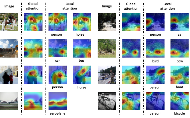
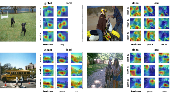
We visualized the attentive areas for the images on PASCAL VOC 2007 by up-sampling the attention weights with a factor of $2^{4}=16$ and applying a Gaussian filter. We showed the predictions and the relative attentive areas of images in Fig. 3 and  4. Fig. 3 represents some visualized results of global and local attention and Fig. 4 shows the trend for attention updating every 10 epochs. From Fig. 3 and  4, we can see when predicting the related labels of an image, the model first observed the image in general (the attentive areas are covered most of the region of the image). Then at each step of RNN, the model focused on smaller areas that may contain specific target objects. This is very similar to human thinking that people observe an image, they always glance the whole image, and then they consider the relationships inside the image, and focus on their attention on some specific objects.

Conclusions

In this paper, we proposed a novel model that uses a global/local attention mechanism for multi-label image classification. In our model, we first let the model focus on a more coarse area of an image, i.e., a global attention on the image. Then, with the guidance of the global attention, the model can predict each label one by one with the local attention, which can attentively help the model focus on some specific objects. Additionally, we proposed a joint max-margin objective that defines two max-margin in vertical and horizontal directions, respectively. Finally, we evaluated our method on two popular multi-label image datasets, i.e., Pascal VOC 2007 and MS-COCO. Our experimental results showed the superiority of the proposed method.

References

- [1] A. Cocchia, “Smart and digital city: A systematic literature review,” in Smart city. Springer, 2014, pp. 13–43.
- [2] K. Su, J. Li, and H. Fu, “Smart city and the applications,” in Electronics, Communications and Control (ICECC), 2011 International Conference on. IEEE, 2011, pp. 1028–1031.
- [3] G. Sanghi, N. Kanungo, S. Deshmukh, and S. Agarwal, “Automatic multi-label image annotation for smart cities,” in IEEE Region 10 Symposium (TENSYMP), 2017. IEEE, 2017, pp. 1–4.
- [4] A. Alhamoud, V. Muradi, D. Böhnstedt, and R. Steinmetz, “Activity recognition in multi-user environments using techniques of multi-label classification,” in Proceedings of the 6th International Conference on the Internet of Things. ACM, 2016, pp. 15–23.
- [5] J. Deng, W. Dong, R. Socher, L.-J. Li, K. Li, and L. Fei-Fei, “Imagenet: A large-scale hierarchical image database,” in Computer Vision and Pattern Recognition, 2009. CVPR 2009. IEEE Conference on. IEEE, 2009, pp. 248–255.
- [6] K. Simonyan and A. Zisserman, “Very deep convolutional networks for large-scale image recognition,” arXiv preprint arXiv:1409.1556, 2014.
- [7] K. He, X. Zhang, S. Ren, and J. Sun, “Deep residual learning for image recognition,” in Proceedings of the IEEE Conference on Computer Vision and Pattern Recognition, 2016, pp. 770–778.
- [8] Y. Gong, Y. Jia, T. Leung, A. Toshev, and S. Ioffe, “Deep convolutional ranking for multilabel image annotation,” arXiv preprint arXiv:1312.4894, 2013.
- [9] A. Krizhevsky, I. Sutskever, and G. E. Hinton, “Imagenet classification with deep convolutional neural networks,” in Advances in Neural Information Processing Systems 25, F. Pereira, C. J. C. Burges, L. Bottou, and K. Q. Weinberger, Eds. Curran Associates, Inc., 2012, pp. 1097–1105.
- [10] A. Sharif Razavian, H. Azizpour, J. Sullivan, and S. Carlsson, “Cnn features off-the-shelf: an astounding baseline for recognition,” in Proceedings of the IEEE Conference on Computer Vision and Pattern Recognition Workshops, 2014, pp. 806–813.
- [11] Y. Wei, W. Xia, J. Huang, B. Ni, J. Dong, Y. Zhao, and S. Yan, “Cnn: Single-label to multi-label,” arXiv preprint arXiv:1406.5726, 2014.
- [12] J. Wang, Y. Yang, J. Mao, Z. Huang, C. Huang, and W. Xu, “Cnn-rnn: A unified framework for multi-label image classification,” in Proceedings of the IEEE Conference on Computer Vision and Pattern Recognition, 2016, pp. 2285–2294.
- [13] J. Jin and H. Nakayama, “Annotation order matters: Recurrent image annotator for arbitrary length image tagging,” arXiv preprint arXiv:1604.05225, 2016.
- [14] F. Liu, T. Xiang, T. M. Hospedales, W. Yang, and C. Sun, “Semantic regularisation for recurrent image annotation,” arXiv preprint arXiv:1611.05490, 2016.
- [15] D. Bahdanau, K. Cho, and Y. Bengio, “Neural machine translation by jointly learning to align and translate,” arXiv preprint arXiv:1409.0473, 2014.
- [16] K. Xu, J. Ba, R. Kiros, K. Cho, A. Courville, R. Salakhudinov, R. Zemel, and Y. Bengio, “Show, attend and tell: Neural image caption generation with visual attention,” in International Conference on Machine Learning, 2015, pp. 2048–2057.
- [17] Z. Zhou, Y. Wang, Q. J. Wu, C.-N. Yang, and X. Sun, “Effective and efficient global context verification for image copy detection,” IEEE Transactions on Information Forensics and Security, vol. 12, no. 1, pp. 48–63, 2017.
- [18] Q. You, H. Jin, Z. Wang, C. Fang, and J. Luo, “Image captioning with semantic attention,” pp. 4651–4659, 2016.
- [19] M.-L. Zhang and Z.-H. Zhou, “A review on multi-label learning algorithms,” IEEE transactions on knowledge and data engineering, vol. 26, no. 8, pp. 1819–1837, 2014.
- [20] M. R. Boutell, J. Luo, X. Shen, and C. M. Brown, “Learning multi-label scene classification,” Pattern recognition, vol. 37, no. 9, pp. 1757–1771, 2004.
- [21] J. Read, B. Pfahringer, G. Holmes, and E. Frank, “Classifier chains for multi-label classification,” Machine Learning and Knowledge Discovery in Databases, pp. 254–269, 2009.
- [22] ——, “Classifier chains for multi-label classification,” Machine learning, vol. 85, no. 3, pp. 333–359, 2011.
- [23] M.-L. Zhang and Z.-H. Zhou, “Ml-knn: A lazy learning approach to multi-label learning,” Pattern recognition, vol. 40, no. 7, pp. 2038–2048, 2007.
- [24] A. Clare and R. D. King, “Knowledge discovery in multi-label phenotype data,” in European Conference on Principles of Data Mining and Knowledge Discovery. Springer, 2001, pp. 42–53.
- [25] J. Lu, J. Yang, D. Batra, and D. Parikh, “Hierarchical question-image co-attention for visual question answering,” in Advances In Neural Information Processing Systems, 2016, pp. 289–297.
- [26] F. Zhu, H. Li, W. Ouyang, N. Yu, and X. Wang, “Learning spatial regularization with image-level supervisions for multi-label image classification,” arXiv preprint arXiv:1702.05891, 2017.
- [27] Z. Pan, P. Jin, J. Lei, Y. Zhang, X. Sun, and S. Kwong, “Fast reference frame selection based on content similarity for low complexity hevc encoder,” Journal of Visual Communication and Image Representation, vol. 40, no. part B, pp. 516–524, 2016.
- [28] S. Hochreiter and J. Schmidhuber, “Long short-term memory,” Neural computation, vol. 9, no. 8, pp. 1735–1780, 1997.
- [29] Z. Yang, Y. Yuan, Y. Wu, W. W. Cohen, and R. R. Salakhutdinov, “Review networks for caption generation,” in Advances in Neural Information Processing Systems, 2016, pp. 2361–2369.
- [30] W. Zaremba and I. Sutskever, “Learning to execute,” arXiv preprint arXiv:1410.4615, 2014.
- [31] M. Everingham, L. Van Gool, C. K. Williams, J. Winn, and A. Zisserman, “The pascal visual object classes (voc) challenge,” International journal of computer vision, vol. 88, no. 2, pp. 303–338, 2010.
- [32] T.-Y. Lin, M. Maire, S. Belongie, J. Hays, P. Perona, D. Ramanan, P. Dollár, and C. L. Zitnick, “Microsoft coco: Common objects in context,” in European Conference on Computer Vision. Springer, 2014, pp. 740–755.
- [33] H. Harzallah, F. Jurie, and C. Schmid, “Combining efficient object localization and image classification,” in Computer Vision, 2009 IEEE 12th International Conference on. IEEE, 2009, pp. 237–244.
- [34] F. Perronnin, J. Sánchez, and T. Mensink, “Improving the fisher kernel for large-scale image classification,” Computer Vision–ECCV 2010, pp. 143–156, 2010.
- [35] T. Jaakkola and D. Haussler, “Exploiting generative models in discriminative classifiers,” in Advances in neural information processing systems, 1999, pp. 487–493.
- [36] B. Gu and V. S. Sheng, “A solution path algorithm for a general parametric quadratic programming problem,” IEEE Transactions on Neural Networks and Learning Systems, vol. 28, no. 5, pp. 1241–1248, 2017.
- [37] B. Gu, X. Sun, and V. S. Sheng, “Structural minimax probability machine,” IEEE Transactions on Neural Networks and Learning Systems, vol. 28, no. 7, pp. 646–1656, 2017.
- [38] B. Gu, V. S. Sheng, K. Y. Tay, W. Romano, and S. Li, “Incremental support vector learning for ordinal regression,” IEEE Transactions on Neural Networks and Learning Systems, vol. 26, no. 7, pp. 1403–1416, 2015.