Extreme Flow Decomposition for Multi-Source Multicast with Intra-Session Network Coding

Abstract

Network coding (NC), when combined with multipath routing, enables a linear programming (LP) formulation for a multi-source multicast with intra-session network coding (MISNC) problem. However, it is still hard to solve using conventional methods due to the enormous scale of variables or constraints. In this paper, we try to solve this problem in terms of throughput maximization from an algorithmic perspective. We propose a novel formulation based on the extereme flow decomposition technique, which facilitates the design and analysis of approximation and online algorithms. For the offline scenario, we develop a fully polynomial time approximation scheme (FPTAS) which can find a $(1+\omega)$-approximation solution for any specified $\omega>0$. For the online scenario, we develop an online primal-dual algorithm which proves $O(1)$-competitive and violates link capacities by a factor of $O(\log m)$, where $m$ is the link number. The proposed algorithms share an elegant primal-dual form and thereby have inherent advantages of simplicity, efficiency, and scalability. To better understand the advantages of the extereme flow decomposition approach, we devise delicate numerical examples on an extended butterfly network. We validate the effects of algorithmic parameters and make an interesting comparison between the proposed FPTAS and online algorithm. The results show that the online algorithm has satisfactory performance while keeping the overall link utilization acceptable compared with the FPTAS.

I Introduction

Among various potential benefits brought by Network Coding (NC), the most significant one is to maximize the multicast throughput in wired networks, or to improve the reliability and hence the unicast throughput in wireless neworks [29]. NC and multipath routing are essential to formulate a multicast optimization problem with Intra-Session Network Coding (ISNC) to a Linear Program (LP) based on the classical Multi-Commodity Flow (MCF) models [1]. Even so, the LP is hard to solve using conventional methods due to the enormous scale of variables or constraints. Naturally, this area of research divides into two major classes: Single-source multicast with ISNC (SISNC) and Multi-source multicast with ISNC (MISNC).

There are volumes of research outputs that optimize multicast performance or analyze the user behaviors in SISNC, while few attention has been paid to the fundamental MISNC problem due to its computation complexity. It is therefore significant to design efficient algorithms that can exactly or approximately solve the LP problem.

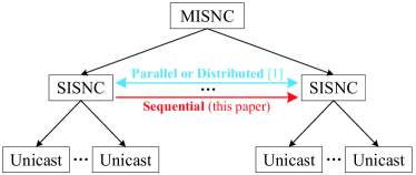
Figure 1: Comparison of approaches used in [1] and this paper.

In our prior work [1], as shown in Fig. 1, we demonstrate that the original MISNC problem can be solved in a two-level decomposition framework. At the upper level, a multi-source multicast is decomposed into a series of single-source multicast and at the lower level, each single-source multicast is further decomposed into a series of unicast. The solution is by nature an exact algorithm features a design philosophy of trading time for space. In this paper, however, we investigate the MISNC problem from the perspective of how to efficiently obtain approximate solutions, which features a design philosophy of trading accuracy for time and space. Moreover, the sequential processing structure enables an online implementation which has great realistic significance. Also, we focus on the upper level in this paper due to practical consideration and analytical tractability. In summary, we aim to tackle the following challenges.

• How to establish computationally tractable model to maximize the multicast throughput by leveraging the linear structural properties of ISNC?

• Further, how to design efficient algorithms to approximately solve the model with performance guarantees in both offline and online scenarios?

The problems are non-trivial due to the fact that the MISNC problem cannot be formulated into path-based or tree-based models using conventional methods, and thus cannot be solved by adapting from existing algorithms designed for gereral MCF problems without NC. More importantly, it is still unclear how to choose a set of multiple multicast trees that is optimal for the objective function [23]. The reasons for this are two-fold: first, the number of multicast trees in a network can be exponentially large; second, the link sharing relationship between different trees caused by NC is intractable [23].

Inspired by the facts that a min-cost SISNC problem can be efficiently solved in a distributed or parallel manner [1, 6], and that a min-cost computation module is convenient to be integrated into a primal-dual scheme [22, 13], we formulate the MISNC problem based on the extreme flow decomposition technique [13] and develop primal-dual algorithms with guaranteed worst case performance for both offline and online settings. Specifically, the contributions are as follows.

• We propose a novel optimization formulation based on the extereme flow decomposition for the MISNC problem, which facilitates the design and analysis of approximation and online algorithms.

• For the offline setting, we develop a fully polynomial time approximation scheme (FPTAS) which can find a $(1+\omega)$-approximation solution for any specified $\omega>0$ in time that is a polynomial function of the network size.

• For the online setting, we develop online algorithms with exact and approximate min-cost computation modules, respectively. Both of them are designed in a primal-dual style and prove to be $O(1)$-competitive and violate link capacities by a factor of $O(\log m)$, where $m$ is the link number.

• We prove the performance bounds for the proposed algorithms and, to better understand the advantages of the extereme flow decomposition, we devise delicate numerical examples on a prototype network to illustrate the effects of the algorithmic parameters and make a direct comparison between the FPTAS and the online algorithm.

The rest of this paper is organized as follows. We review related work in Section II. We introduce the system model and assumptions in Section III. We formulate the offline and online MISNC problems and develop approximation and online algorithms in Sections IV and V, respectively, followed by the crucial min-cost computation modules in Section VI. We then present numerical examples in Section VII. Finally, we conclude in Section VIII. All proofs are presented in the appendix. Main notation is summarized in Table I.

II Related Work

II-A Intra-Session Network Coding (ISNC)

ISNC is recently attracting public attention with the prolifiration of new generation of wireless networks. Xu et al. [28] employ network coding and coalition game theory to jointly optimize the network throughput and content service satisfaction degree in mobile edge computing networks. Wang et al. [27] propose a cooperative multicast for layered streaming in a heterogeneous D2D-enhanced cellular network. Malathy et al. [26] present a mixed routing scheme which combines network coding and backpressure routing in a large-scale IoT network. In this scheme, network coding is used to minimize the network congestion, reduce the redundant packets, and enhance the throughput. Zhu et al. [30] propose a Miss-and-Forward paradigm for ISNC, where a relay node is assigned to exploit the space diversity. ISNC is also combined with the opportunistic routing to improve the reliability and throughput in multi-hop wireless networks [29].

Regarding the wired networks, existing works mainly focus on the SISNC problems partly because of the tractable scale of LP formulations for such case [6, 4, 5]. These works can be roughly classified into two categaries. First, all the receivers of a multicast are assumed to cooperate with each other to reach some global traffic engineering objectives, such as minimum cost, maximum throughput, minimum Maximum Link Utilization (MLU). Second, each multicast receiver is assumed to be selfish and greedily routes its flows, thus whether there exists an equilibrium needs to be considered.

The considered MISNC problem falls into the first class and for this problem, only heuristics [2], approximation algorithms [8] with no desirable performance guarantees, and suboptimal solutions [9] are proposed. In [1], we formulated an LP for the MISNC problem in order to minimize the MLU. We then presented a dual-dual decomposition approach [10] whereby the original problem is decomposed into a series of minimum-cost flow subproblems plus a centralized computation. As such, the subproblems can be efficiently solved in a parallel or decentralized manner.

Essentially, the key components are all to solve a set of multicast optimization problems. The decomposition in [1] occurs in spatial dimension, where multiple multicast requests can be processed simultaneously by different computation entities, or can of course be processed sequencially by the same computation entity. In this paper, the decomposition occurs in temporal dimension, where multiple multicast requests must be processed sequencially, although the order is not important. On the other hand, the decomposition method in [1] is by nature an exact algorithm which aims to trade time for space. The centralized computation part involves a somewhat inefficient subgradient iteration module over a convex set. The proposed algorithms in this paper are by nature approximation algorithms which sacrifice accuracy for computation efficiency. We can use an appropriately chosen parameter to reach a trade-off in practice. In both of the two decomposition methods, however, the updates of dual link weights at the upper level should be executed in a centralized manner.

II-B Primal-Dual Algorithms for Network Flow Problems

The primal-dual scheme has been employed to solve a variety of MCF-based network flow problems [7], including both approximation algorithms and online algorithms. According to the problem sturctures, different meta-structures, i.e., the basic routing units, are taken into account, see Table II.

A long line of works have addressed the design of FPTAS for MCF under unicast scenarios [22, 21, 12]. For multicast, Sengupta et al. [14] develop a family of FPTASs that can maximize multicast streaming capacity and corresponding multicast trees in node capacitated P2P networks. The algorithms involve smallest price tree construction in the innermost loops. Kodialam et al. [15, 16] adapt the FPTAS to maximize the achievable rates in multi-hop wireless networks by jointly considering routing and scheduling problems. The major difference is that the capacity constraint is specially designed for the wireless mesh nodes, and is flexible enough to handle various wireless interference conditions and channel models. Bhatia et al. [17] present FPTAS to maximize the throughput with fast restoration against link and node failures. However, the generic path, used as the meta-structure, is no longer a simple path but consists of a primary path and a backup detour. Agarwal et al. [3] formulate the SDN controller optimization problem for traffic engineering with evolutinary deployment of SDN routing devices and develop an FPTAS for solving the problem. In recent years, many works extend the shortest-path or min-cost tree based algorithms to design policy-aware routing algorithms that steer network flows through predefined service function chains under network function virtualizaiton environment in order to maximize the total flow demands [18, 19, 20]. Bhatia et al. [24] design FPTAS and online primal-dual algorithms to determine the optimal parameters for segment routing in both offline and online settings, and also consider the restoration from node or link failures [25].

Unlike the above works, we treat each SISNC as an MCF, or equivalently, a feasible extreme flow in the flow polytope [13]. In this way, the proposed FPTAS features a two-level (phase-iteration) structure which outperforms the three-level (phase-iteration-step) structures due to a substantial reduction in the number of loops as well as in running time. The proposed online algorithm also benefits from this and thus achieve a disirable network throughput because multipath routing is inherently supported.

III System Model

Let $G=(V,E)$ be a directed network, where $V$ is the node set and $E$ is the link set. The number of nodes and links are denoted by $n$ and $m$, respectively. There are a set of multicast requests $R$ to be transmitted through the network. Each request $r\in R$ is associated with one source $s_{r}\in V$ and a set $T_{r}\in V$ of receivers. We assume that all receivers in $T_{r}$ receive service at the same rate $d_{r}$ from $s_{r}$.

TABLE I: Notations

Notation	Description
$G=(V,E)$	A directed network where $V$ represents the node set and $E$ the link (edge) set.
$n,m$	Node number and link number of $G$, respectively.
$r$	Request $r$.
$R,|R|$	Request set $R$ and its cardinality.
$s_{r}$, $T_{r}$	Source node and target node set of request $r$.
$d_{r}$	Size of request $r$.
$c_{e}$	Capacity of link $e$.
${{\Pi}_{r}}$	Flow polytope for request $r$.
$V({\Pi_{r}})$	Set of extreme flows (extreme points) of ${{\Pi}_{r}}$.
$f_{e}$	Flow value that an extreme flow $f$ imposes on link $e$.
${x_{r}^{f}}$	Flow amount of request $r$ routed as a scaled extreme flow $f$.
${X_{r}^{f}}$	Integer indicating whether a request $r$ has been accepted to route as a scaled extreme flow $f$.
$x_{e}$	Total flow value on link $e$.
$p_{e}$	Dual variable associated with each link $e$.
$z_{r}$	Dual variable associated with each request $r$.
$\lambda$	Maximum multiplier such that multicast rate $\lambda{{d}_{r}}$ can be supported for $r$.
$\epsilon$	Global tunable parameter of FPTAS.
$\phi$	Global tunable parameter of online algorithm.
LP	Linear program.
MCF	Multi-commodity flow.
ISNC	Intra-session network coding.
SISNC	Single-source multicast with ISNC.
MISNC	Multi-source multicast with ISNC.
FPTAS	Fully polynomial time approximation scheme.

III-A Intra-Session Network Coding (ISNC)

To focus on the major challenges, we make the following assumptions in this paper.

• Solving the problem includes two decoupled stages: first, computing the routing subgraph; second, determining the random coding scheme on the routing subgraph [11, 6]. We concentrate on the former and do not go deep into the coding details.

• We assume that NC is only allowed within a multicast request (ISNC) and disallowed among different multicast requests because of the impracticability and computational intractability [1, 4].

Under the second assumption, the MISNC model can be viewed as a group of SISNC coupled by link capacity constriants. The following theorem summarizes the most important property for an SISNC.

Theorem 1: In a directed network with network coding, a multicast rate is feasible if and only if it is feasible to each receiver independently. When using random linear coding schemes, there is a fully decentralized approach to achieve the min-cost multicast with strictly convex cost functions.

Proof: Refer to [6]. ∎

III-B Extreme Flow Decomposition

We adapt some definitions on the extreme flow decomposition in [13] to our problem as follows.

Definition 1: For each multicast request $r=({{s}_{r}},{{T}_{r}},{{d}_{r}})$, ${{\Pi}_{r}}$ denote the flow polytope of unit flows $f$ (i.e., $|f|=1$) from $s_{r}$ to $T_{r}$ in $G$ that satisfy: ${{f}_{e}}\leq\frac{{{c}_{e}}}{{{d}_{r}}},\forall e$. We say that request $r$ is feasible if ${{\Pi}_{r}}\neq\varnothing$.

Definition 2: The set of extreme flows (extreme points) of ${{\Pi}_{r}}$ is denoted by $V({\Pi_{r}})$. Each extreme point represents a feasible flow which must saturates some links. Any feasible flow can be represented by the linear combination of extreme flows.

The comparison of various decomposition methods is given in Table II. When designing a primal-dual algorithm, the path or tree decomposition has a three-level (phase-iteration-step) structure, while the extreme flow decomposition has a two-level (phase-iteration) structure.

TABLE II: Comparison of various decomposition methods

Strategy	Meta-structure	Routing	Computation	Feasible flow
Path decomposition	path	shortest path	unicast	sum of path flows
Tree decomposition	tree	Steiner tree	multicast	sum of tree flows
Extreme flow decomposition	extreme flow	min-cost MCF	unicast, multicast (ISNC)	linear combination of extreme flows

IV Offline Network Throughput Maximization

In the offline setting, we asume all the multicast requests are known in advance. The objective is to simultaneously maximize the multicast throughput of all the requests. We first present the offline formulation and then develop an approximation algorithm.

IV-A Problem Formulation

Similar to the well-kwown maximum concurrent flow problem [22], the objective is to find the largest $\lambda$ such that there is an MCF which routes at least $\lambda{{d}_{r}}$ for all requests $r$. Thus, the problem can be formulated as the following LP.

max $$\lambda (P_{\rm off})$$

s.t. $$\sum\limits_{f\in V({{\Pi}_{r}})}{{{y}_{f}}}\geq\lambda{{d}_{r}}, \forall r.$$ (1)

$$\sum\limits_{r}{\sum\limits_{f\in V({{\Pi}_{r}})}{{{f}_{e}}{{y}_{f}}}}\leq{{c}_{e}}, \forall e.$$ (2)

$${{y}_{f}}\geq 0, \forall r,\forall f\in V({{\Pi}_{r}}).$$

$$\lambda\in\mathbb{R}.$$

Similar to a typical MCF formulation, constraints (1) and (2) imply the flow conservation and capacity limitation, respectively. By associating a price $p_{e}$ with each link $e$ and a weight $z_{r}$ with each request $r$, we write the dual to the above LP as:

min $$D(p):=\sum\limits_{e}{{{p}_{e}}{{c}_{e}}} (D_{\rm off})$$

s.t. $$\sum\limits_{e}{{{p}_{e}}{{f}_{e}}}\geq{{z}_{r}}, \forall r,\forall f\in V({{\Pi}_{r}}).$$ (3)

$$\sum\limits_{r}{{{z}_{r}}{{d}_{r}}}\geq 1.$$ (4)

$$z_{r}\geq 0, \forall r.$$

$${p_{e}}\geq 0, \forall e.$$

Recall that a flow polytope may have exponentially many vertices. Thus in the worst case, there could be at most exponential number of variables in $(P_{\rm off})$. As far as we know, no tractable general-purpose LP solver can be directly applied to such problem even for a medium sized network.

IV-B Approximation Algorithm

We design an FPTAS to solve the problem. The FPTAS is a primal-dual algorithm which includes an outer loop of a primal-dual update and an inner loop of min-cost MCF path computation.

The algorithm to solve the problem starts by assigning a precomputed price of $\frac{\delta}{{{c_{e}}}}$ to all links $e$.

The algorithm proceeds in phases. In each phase, we route $d_{r}$ units of flow from node $s_{r}$ to $T_{r}$ for each multicast request $r$. A phase ends when all multicast requests are routed.

The flow of value $d_{r}$ of request $r$ is routed from $s_{r}$ to $T_{r}$ in multiple iterations as follows. In each iteration, a min-cost MCF path with unit request size from $s_{r}$ to $T_{r}$ that minimizes the left-hand side of constraint (3) under current link prices is computed.

The path is computated in Section VI. The amount of flow sent along this path in an iteration is $d_{r}$.

After the flow of value $d_{r}$ is sent along the MCF path, the flow value and the link price at each link along the path $f^{*}$ are updated as follows:

1) Update the flow value $x_{e}$ as

$${x_{e}}\leftarrow{x_{e}}+{f^{*}_{e}}{d_{r}}$$

2) Update the link prices $p_{e}$ as

$${{p}_{e}}\leftarrow{{p}_{e}}\left(1+\epsilon\frac{{f^{*}_{e}}{d_{r}}}{{{c}_{e}}}\right)$$

The update happens after each iteration associated with routing a complete request $d_{r}$. The algorithm terminates when the dual objective function value $D(p)$ becomes less than one.

When the algorithm terminates, dual feasibility constraints will be satisfied. However, link capacity constraints (2) in the primal solution will be violated, since we were working with the original (not the residual) link capacities at each stage. To remedy this, we scale down the traffic at each link uniformly so that the link capacity constraints are satisfied.

Note that unlike the existing three-level FPTASs, FPTAS ISNC needs not to compute a bottleneck, or maximum allowable flow rate in the flow value update since in the Min-Cost SISNC Computation module the link capacities have been scaled down by a factor $d_{r}$.

Theorem 2: For any specified $\omega>0$, Algorithm 1 computes a $(1+\omega)$-approximation solution. If the algorithmic parameters are $\epsilon(\omega)=1-{{(1+\omega)}^{-\frac{1}{3}}}$ and $\delta(\omega)={{\left(\frac{1-\epsilon}{m}\right)}^{\frac{1}{\epsilon}}}$, the running time is $O\left(\frac{|R|\log|R|}{\epsilon}{{\log}_{1+\epsilon}}\frac{m}{1-\epsilon}{{{T_{{\rm{NC}}}}}}\right)$, where $T_{\rm{NC}}$ is the time required to compute a min-cost unit MCF for SISNC.

Proof: See Appendix. ∎

Algorithm 1 FPTAS for MISNC

  Input: ${p_{e}}\leftarrow\frac{\delta}{{{c_{e}}}},\forall e$; $x_{e}\leftarrow 0,\forall e$; $\rho\leftarrow 0$

  while $D(p)<1$ do

     for $\forall r\in R$ do

        Invoke Algorithm 4 to compute the min-cost unit MCF from $s_{r}$ to $T_{r}$ in $G$ under the link price system $p$. Denote $f^{*}$ as the min-cost unit MCF.

        for $\forall e\in f^{*}$ do

           ${x_{e}}\leftarrow{x_{e}}+{f^{*}_{e}}{d_{r}}$

           ${{p}_{e}}\leftarrow{{p}_{e}}\left(1+\epsilon\frac{{f^{*}_{e}}{d_{r}}}{{{c}_{e}}}\right)$

        end for

     end for

     $\rho\leftarrow\rho+1$

     $D(p)\leftarrow\sum\limits_{e}{{p_{e}}{c_{e}}}$

  end while

  ${x_{e}}=\frac{{{x_{e}}}}{{{{\log}_{1+\epsilon}}\frac{{1}}{\delta}}},\forall e$

  $\lambda=\frac{{\rho-1}}{{{{\log}_{1+\epsilon}}\frac{1}{\delta}}}$

  Output: ${x_{e}}$; $\lambda$

V Online Network Throughput Maximization

In the online setting, the multicast requests arrive one by one without the knowledge of future arrivals. The objective is to accept as many multicast requests as possible. We first formulate the online problem and then develop an online primal-dual algorithm.

V-A Problem Formulation

Based on the maximum multicommodity flow problem [22], the online problem can be formulated as the following ILP.

max $$\sum\limits_{r}{{{d}_{r}}\sum\limits_{f\in V({{\Pi}_{r}})}{X_{r}^{f}}} (P_{\rm on})$$

s.t. $$\sum\limits_{f\in V({\Pi_{r}})}{X_{r}^{f}}\leq 1, \forall r.$$ (5)

$$\sum\limits_{r}{{{d}_{r}}\sum\limits_{f\in V({{\Pi}_{r}})}{{{f}_{e}}X_{r}^{f}}}\leq{{c}_{e}}, \forall e.$$ (6)

$$X_{r}^{f}\in\{0,1\}, \forall r,\forall f\in V({{\Pi}_{r}}).$$

Similar to the offline formulation, constraints (5) and (6) imply the flow conservation and capacity limitation, respectively. The integer $X_{r}^{f}$ indicates whether or not a request $r$ has been accepted to route as a scaled extreme flow $f$. We then consider the LP relaxation of this problem where $X_{r}^{f}\in\{0,1\}$ is relaxed to $X_{r}^{f}\geq 0$. Note that $X_{r}^{f}\leq 1$ is already implied by constraint (5). By associating a price $p_{e}$ with each link $e$ and a weight $z_{r}$ with each request $r$, we can write the dual to the above LP as:

min $$\sum\limits_{r}{{z_{r}}}{\rm{+}}\sum\limits_{e}{{p_{e}}{c_{e}}} (D_{\rm on})$$

s.t. $${z_{r}}\geq{d_{r}}\left({1-\sum\limits_{e}{{p_{e}}{f_{e}}}}\right), \forall r,\forall f\in V({\Pi_{r}}).$$ (7)

$$z_{r}\geq 0, \forall r.$$

$${p_{e}}\geq 0, \forall e.$$

V-B Online Algorithm

We design an online primal-dual algorithm which includes an outer loop of a primal-dual update and an inner loop of min-cost MCF path computation.

The algorithm to solve the problem starts by assigning a precomputed price of zero to all links $e$.

The algorithm proceeds in iterations and each iteration corresponds to a request. Upon the arrival of a new request $r$, we try to route $d_{r}$ units of flow from node $s_{r}$ to $T_{r}$, for each multicast request $r$.

In each iteration, a min-cost MCF path with unit request size from $s_{r}$ to $T_{r}$ that maximizes the right-hand side of constraint (7) under current link prices computed according to Section VI.

If the min-cost value is larger than one, the request is rejected. Otherwise, the request is accepted, and the entire flow $d_{r}$ of request $r$ is routed along the min-cost MCF path.

After the flow is sent, the flow value and the link price at each link along the path $f^{*}$ are updated as follows:

1) Update the flow value $X_{r}^{{f}}$ as

$$X_{r}^{{f^{*}}}\leftarrow 1,$$

which implies $X_{r}^{f}=0,\forall f\neq{f^{*}}$ according to constraint (5).

2) Update the link prices $p_{e}$ as

$${p_{e}}\leftarrow{p_{e}}\left({1+\frac{{{f^{*}_{e}}{d_{r}}}}{{{c_{e}}}}}\right){\rm{+}}\frac{\phi}{{m}}\frac{{{f^{*}_{e}}{d_{r}}}}{{{c_{e}}}},\phi>0$$

Parameter $\phi$ is designed to provide a tradeoff between the competitiveness of the online algorithm and the degree of violation of the capacity constraints. That is, a smaller $\phi$ leads to larger network throughput as well as a larger degree of violation on the link capacities [19].

Definition 3: If the MCF generated by an online algorithm is $\alpha$-competitive and violates the link capacity constraints by at most $\beta$, the online algorithm is said to be $\left\{\alpha,\beta\right\}$-competitive. $\alpha$ and $\beta$ are also called competitive ratio and violation ratio, respectively.

Theorem 3: Algorithm 2 is an all-or-nothing, non-preemptive, monotone, and $\left\{{O\left(1\right),O\left({\log m}\right)}\right\}$-competitive, more specifically $\left\{{{{1+\phi}},\log\left({\frac{{Bm}}{\phi}+1}\right)}\right\}$-competitive, online algorithm.

Proof: See Appendix. ∎

Algorithm 2 Online Algorithm for MISNC

  Input: $p_{e}\leftarrow 0,\forall e$

  while Upon the arrival of request $r$ do

     Invoke Algorithm 4 to compute the min-cost unit MCF from $s_{r}$ to $T_{r}$ in $G$ under the link price system $p$. Denote $f^{*}$ as the min-cost unit MCF.

     if $L>1$ then

        Reject $r$;

     else

        Accept $r$;

        $X_{r}^{{f^{*}}}\leftarrow 1$

        ${z_{r}}\leftarrow{d_{r}}\left({1-L}\right)$

        for $\forall e\in f^{*}$ do

           ${p_{e}}\leftarrow{p_{e}}\left({1+\frac{{{f^{*}_{e}}{d_{r}}}}{{{c_{e}}}}}\right){\rm{+}}\frac{\phi}{{m}}\frac{{{f^{*}_{e}}{d_{r}}}}{{{c_{e}}}}$,

           where $\phi>0$.

        end for

     end if

  end while

  Output: $X_{r}^{f}$

V-C Online Algorithm with Flow Shifting

The modified online algorithm, as presented in Algorithm 3, has a similar structure to Algorithm 2. The parameters $\eta$, $\sigma$ (and $\sigma:=\max{\{\eta,\mu\}}$) will be determined in Section VI-B.

Theorem 4: Algorithm 3 is an all-or-nothing, non-preemptive, monotone, and $\left\{{O\left(1\right),O\left({\log m}\right)}\right\}$-competitive, more specifically $\left\{{1+\frac{\phi}{\sigma},\sigma\log\left({\frac{{Bm}}{\phi}+1}\right)}\right\}$-competitive, online algorithm.

Proof: See Appendix. ∎

It is obvious that Algorithm 3 has lower competitve ratio but higher violation ratio than Algorithm 2. However, the difference can only be reflected in theoretical analysis.

Algorithm 3 Online Algorithm for MISNC with Flow Shifting

  Input: $p_{e}\leftarrow 0,\forall e$

  while Upon the arrival of request $r$ do

     Invoke Algorithm 5 to compute the min-cost unit MCF from $s_{r}$ to $T_{r}$ in $G$ under the link price system $p$. Denote $f^{*}$ as the min-cost unit MCF.

     if $L>\lambda$ then

        Reject $r$;

     else

        Accept $r$;

        $X_{r}^{{f^{*}}}\leftarrow 1$

        ${z_{r}}\leftarrow{d_{r}}\left({1-\frac{L}{\sigma}}\right)$

        for $\forall e\in f^{*}$ do

           ${p_{e}}\leftarrow{p_{e}}\left({1+\frac{{{f^{*}_{e}}{d_{r}}}}{{\sigma{c_{e}}}}}\right){\rm{+}}\frac{\phi}{{m}}\frac{{{f^{*}_{e}}{d_{r}}}}{{\sigma{c_{e}}}}$,

           where $\phi>0$.

        end for

     end if

  end while

  Output: $X_{r}^{f}$

VI Min-Cost SISNC Computation

For the primal-dual algorithms in both offline and online cases, efficiently computing a min-cost MCF for a given price system is the key module in each iteration. The min-cost NC muilticast problem can be solved, either exactly or approximately, in many ways, such as optimization decomposition techniques or general LP solvers. In this section, we give an exact version of Min-Cost SISNC Computation in Algorithm 4 and an approximate version in Algorithm 5. The former is integrated into the FPTAS and the online algorithm while the latter is only for the online algorithm.

VI-A Exact Min-Cost SISNC Computation

According to [1, 6], the min-cost SISNC problem can be formulated as the following LP.

min $$\sum\limits_{e}{{{p}_{e}}{{f}_{e}}} (MNC)$$

s.t. $$\sum\limits_{p\in{{P}_{i}}}{f(p)}=1, \forall i.$$ (8)

$${{f}_{i,e}}:=\sum\limits_{e\in p\in{{P}_{i}}}{f(p)}\leq{{f}_{e}}, \forall i,\forall e.$$ (9)

$${f_{e}}\leq\frac{{{c_{e}}}}{{{d_{r}}}}, \forall e.$$ (10)

$$f(p), \forall p.$$

$${{f}_{e}}, \forall e.$$

Constraint (8) follows the rule of flow conservation with unit flow request. The index $i$ indicates a unicast from $s_{r}$ to one of the multicast receivers $i\in{T_{r}}$ and $P_{i}$ represents the path set of this unicast. Constraint (9) means that the conceptual link flow $f_{i,e}$ is constrained by the actual link flow $f_{e}$. This constraint characterizes the NC multicast. Constraint (10) ensures that the actual link flow $f_{e}$ is constrained by the scaled link capacity. Any feasible solution $f_{e}$ of problem (MNC) constitutes a unit multicast flow polytope ${{\Pi}_{r}}$ for request $r$.

Algorithm 4 Exact Min-Cost SISNC Computation

  Input: $G$; $r$; $p$

  Solve the problem (MNC) by invoking the decomposition algorithm in [6] or using an LP solver.

  The minimum cost of the unit MCF is:

   $L:=\mathop{\min}\limits_{f\in V({\Pi_{r}})}\sum\limits_{e}{{p_{e}}{f_{e}}}$

  The min-cost unit MCF is:

   $f^{*}:=\arg\mathop{\min}\limits_{f\in V({\Pi_{r}})}L$

  Output: $f^{*}$; $L$

Algorithm 5 Approximate Min-Cost SISNC Computation

  Input: $G$; $r$; $p$

  Solve the problem (MNC) by invoking the decomposition algorithm in [6] or using an LP solver.

  The minimum cost of the unit MCF is:

   $L:=\mathop{\min}\limits_{f\in V({\Pi_{r}})}\sum\limits_{e}{{p_{e}}{f_{e}}}$

  The min-cost unit MCF is:

   $f^{*}:=\arg\mathop{\min}\limits_{f\in V({\Pi_{r}})}L$

  for $\forall i\in{T_{r}}$ do

     Shift the path flows smaller than $\frac{1}{{2{w_{i}}^{2}}}$ to other flow paths from $s_{r}$ to $i$ according to the rules in [13].

  end for

  Update $f^{*}$ and $L$.

  Output: $f^{*}$; $L$

VI-B Approximate Min-Cost SISNC Computation

Algorithm 5 is in essence an approximate algorithm. It produces a solution where the min-cost value $L$ is at most $\eta$ times the optimum and the link loads of $f^{*}$ are at most $\mu$ times the link capacities. In the following, we call it a $(\eta,\mu)$-criteria algorithm. Based on this criteria, Algorithm 4 can be regarded as a $(1,1)$-criteria algorithm.

The core of Algorithm 5 is a simple flow shifting manipulation based on the outputs of Algorithm 4 . Denote the number of paths from $s_{r}$ to $i\in{T_{r}}$ by $w_{i}$. For each unicast from $s_{r}$ to $i$, shift the path flows smaller than $\frac{1}{{2{w_{i}}^{2}}}$ to other flow paths according to [13]. Since different unicast flows in an NC multicast can overlap with each other when sharing the link capacity, implied by constraints (9) and (10), the min-cost approximation ratio and the capacity violation ratio are identical to the unicast MCF case in [13], i.e., $\eta=\mu=2$.

Definition 4: Define the granularity ${F_{{\rm{min}}}}$ as the smallest link load value of $f^{*}$ [13]. In both of Algorithm 4 and Algorithm 5, ${F_{{\rm{min}}}}$ is a constant.

Theorem 5: In Algorithm 5, ${F_{{\rm{min}}}}$ is lower bounded by $\frac{1}{{2{w_{\max}}^{2}}}$, i.e.: ${F_{{\rm{min}}}}{\rm{\geq}}\frac{1}{{2{w_{\max}}^{2}}}$, where ${w_{\max}}=\mathop{\max}\limits_{i\in{T_{r}}}{w_{i}}$. Further, Algorithm 5 is a $(2,2)$-criteria algorithm.

Proof: Refer to [13]. ∎

As can be seen in the Appendix, the introduction of granularity is to upper bound the dual link price variables, and implies that a flow between a node pair should not be split into too many tiny sub flows. This generally holds in practice and is indispensable to prove the primal feasibility of the online algorithm. The flow shifting operation is designed to further lower bound the granularity for theoretical analysis and thereby makes Algorithm 3 less practical due to large implementation and computation overheads [13].

VII Numerical Examples

Considering that the proposed algorithms prove to run in polynomial time and have provable worst case performance and that we hope to clearly show the flow distribution over all the network links for ease of analysis, we use a prototype network for the MISNC problem, see Fig. 2, which is modified from the classical butterfly network [1, 9]. We use this network because it can clearly shows the nature of ISNC. That is, it is enough to characterize the link sharing within the same multicast session and the link competition between different multicast sessions. More importantly, it is also convenient to verify the correctness of our solutions since the optimum can be easily computed.

All network links have the same capacities 100 and the same weights 1. There are two type of multicast requests $r_{1}$ and $r_{2}$ to be transmitted. The source node sets and sink node sets are $s_{r_{1}}=\{1\}$, $T_{r_{1}}=\{8,10\}$ and $s_{r_{2}}=\{2\}$, $T_{r_{2}}=\{10,12\}$, respectively.

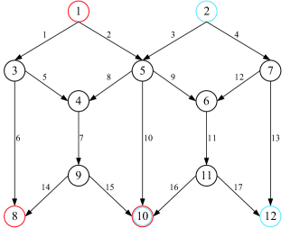
Figure 2: Testing topology [1]. Link indices are the numbers next to the links.

VII-A Offline Setting

Fig. 3 validates the parameter $\epsilon$ in terms of the routing performance metric $\lambda$ and the computation cost metric. The normalized computation time is defined as the ratio of real computation time to the real computation time when $\epsilon=0.1$ (a commonly used setting in literature). In the offline setting, the request size is set as $d_{r_{1}}=d_{r_{2}}=150$. Thus, the optimal value of $\lambda$ is exactly 1.

In Fig. 3, we can see that when $\epsilon$ decreases, $\lambda$ grows linearly while the computation time grows exponentially. The setting $\epsilon=0.1$ can reach a tradeoff between routing performance and computation cost.

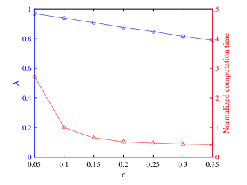
Figure 3: FPTAS. The optimal value of $\lambda$ is 1. The computation time under $\epsilon=0.1$ is used to normalize all the other settings of $\epsilon$.

VII-B Online Setting

Fig. 4 validates the parameter $\phi$ in terms of the routing performance metric acceptance ratio and the resource cost metric violation ratio. The acceptance ratio is defined as the ratio of accepted number of requests to the total request number. The violation ratio is defined as the maximum ratio of the real flow amount on a link to its capacity over all links. It can be obviously seen that the performance bottleneck is link 10, which dominates the violation ratio.

In the online setting, we generate 100 requests for request type 1 and 100 requests for request type 2. Without loss of generality, we make these requests have equal size $d_{r_{1}}=d_{r_{2}}=1.5$. All the 200 requests are randomly ordered and will be injected to the network one by one.

We reuse this request sequence in different $\phi$ values for the sake of fairness. Each multicast request is injected in the network at the ingress node 1 or 2, and is accepted if received by node set {8,10} or {10,12}, respectively.

From Fig. 4, if the capacity constraints are fully respected, the online algorithm when $\phi=4$ can reach an acceptance ratio of around 0.8, which is entirely satisfactory for an online setting.

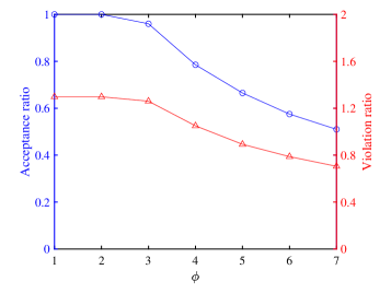
Figure 4: Online algorithm. A violation ratio larger than one means that the flow value on some link exceeds its capacity.

VII-C Comparison between the Two Settings

The two algorithms share a common primal-dual structure. The requests are processed one by one over a long time scale. We make delicate parameter settings for ease of comparison when testing the two algorithms. Specifically, the total request size 100 in the online setting equals to that in the offline setting.

Fig. 5 compares the link utilization between the two algorithms. As a whole, the link utilization of the online algorithm is quite close to that of the FPTAS. The online algorithm when $\phi=1$ accepts all the 200 requests at the cost of a noticable increase in link utilization, and thus in a violation ratio of around 1.2, with the bottleneck link 10.

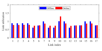
Figure 5: Comparison of link load. Offline ($\epsilon=0.1$). Online ($\phi=1$).

VIII Conclusion

In this paper, we investigate the MISNC problem in terms of throughput maximization. With the help of the extreme flow decomposition technique, we propose an FPTAS and online primal-dual algorithms for offline and online settings, respectively. All the proposed algorithms have provable performance guarantees. Numerical examples show that the FPTAS can asymptotically approach the optimum, and the online algorithm can achieve a desirable trade-off between the routing performance and the resource constraints violation.

As one of our future works, we aim to develop a min-cost version of FPTAS to replace the SISNC computation module used in this paper. We believe this can further accelerate the whole computation process.

Appendix

VIII-A Proofs for Algorithm 1

Lemma 1: When the FPTAS terminates, the primal solution needs to be scaled by a factor of at most ${\log_{1+\epsilon}}\frac{1}{\delta}$ to ensure primal feasibility (i.e., satisfying link capacity constraints).

Proof: Serialize all the iterations of all the phases into $l$ iterations. Define the flow scaling factor of link $e$ as:

$$\kappa:=\sum\limits_{i=1}^{l}{\frac{{{d_{r}^{(i)}}f_{e}^{(i)}}}{{{c_{e}}}}}$$

According to the update rule of $p_{e}$, we have:

$$p_{e}^{\rho-1,K}=\frac{\delta}{{{c_{e}}}}\prod\limits_{i=1}^{l}{\left({1+\epsilon\frac{{{d_{r}^{(i)}}f_{e}^{(i)}}}{{{c_{e}}}}}\right)}$$

Using the Taylor Formula, the inequality ${(1+x)^{a}}\leq 1+ax,\forall x,\forall a\in[0,1]$ holds. Setting $x=\epsilon$ and $a=\frac{{{d_{r}^{(i)}}f_{e}^{(i)}}}{{{c_{e}}}}\leq 1$, we have:

$$1>{c_{e}}p_{e}^{\rho-1,K} \geq\delta\prod\limits_{i=1}^{l}{{{\left({1+\epsilon}\right)}^{\frac{{{d_{r}^{(i)}}f_{e}^{(i)}}}{{{c_{e}}}}}}}$$

$${=}\delta{\left({1+\epsilon}\right)^{\sum\limits_{i=1}^{l}{\frac{{{d_{r}^{(i)}}{f_{e}^{(i)}}}}{{{c_{e}}}}}}}$$

$${=}\delta{\left({1+\epsilon}\right)^{\kappa}}$$

Hence, the lemma is proven.

$$\kappa<{\log_{1+\epsilon}}\frac{1}{\delta}$$

∎

Lemma 2: At the end of $\rho$ phases in the FPTAS, we have

$$\frac{\beta}{{\rho-1}}\leq\frac{\epsilon}{{(1-\epsilon)\ln\frac{{1-\epsilon}}{{m\delta}}}}$$

Proof: For a given $p$, $z_{j}$ is the minimum cost of shipping $d_{j}$ units of flow from $s_{j}$ to $T_{j}$ under price function $p$; henceforth denoted by ${\rm{mincost}}_{j}({p})$, i.e.:

$${\rm{mincost}}_{j}({p})=\mathop{\min}\limits_{f\in V({\Pi_{j}})}\sum\limits_{e}{p_{e}{f_{e}}}$$

Define

$$\alpha(p):=\sum\limits_{j=1}^{K}{{d_{j}}{\rm{mincos}}{{\rm{t}}_{j}}(p)}$$

$$D({p^{i,j}}) =\sum\limits_{e}{{c_{e}}p_{e}^{i,j}}$$

$$=D(p_{e}^{i,j-1})+\epsilon{d_{j}}\sum\limits_{e}{p_{e}^{i,j-1}f_{e}^{i,j}}$$

$$=D({p^{i,j-1}})+\epsilon{d_{j}}{\rm{mincos}}{{\rm{t}}_{j}}({p^{i,j-1}})$$

We now sum over all iterations during phase $i$ to obtain:

$$D({p^{i,K}}) {\leq}D({p^{i,0}})+\epsilon\sum\limits_{j=1}^{K}{{d_{j}}{\rm{mincos}}{{\rm{t}}_{j}}({p^{i,K}})}$$

$${=}D({p^{i,0}})+\epsilon\alpha({p^{i,K}})$$

$${=}D({p^{i-1,K}})+\epsilon\alpha({p^{i,K}})$$

Since $\beta\leq\frac{{D({p^{i,K}})}}{{\alpha({p^{i,K}})}}$, we have:

$$D({p^{i,K}})\leq\frac{{D({p^{i-1,K}})}}{{1-\frac{\epsilon}{\beta}}}$$

Using the initial value $D({p^{1,0}})=m\delta$, we have for $i\geq 1$

$$D({p^{i,K}})\leq\frac{{m\delta}}{{1-\epsilon}}{e^{\frac{{\epsilon(i-1)}}{{\beta(1-\epsilon)}}}}$$

The last step uses the assumption that $\beta\geq 1$. The procedure stops at the first phase $\rho$ for which

$$1\leq D({p^{\rho,K}})\leq\frac{{m\delta}}{{1-\epsilon}}{e^{\frac{{\epsilon(\rho-1)}}{{\beta(1-\epsilon)}}}}$$

which implies that

$$\frac{\beta}{{\rho-1}}\leq\frac{\epsilon}{{(1-\epsilon)\ln\frac{{1-\epsilon}}{{m\delta}}}}$$

∎

Proof of Theorem 2: The analysis of the algorithm proceeds as in [22, 14]. Since the constraints are based on extreme flows and are related to MISNC, the analysis is different.

1) Approximation ratio: We use $\gamma$, the ratio of the dual to the primal objective function values, to upper bound and represent the approximation ratio. Then we have

$$\frac{\mathcal{D}}{\mathcal{P}}:=\gamma<\frac{\beta}{\rho-1}{{\log}_{1+\epsilon}}\frac{1}{\delta}$$

Substituting the bound on $\frac{\beta}{\rho-1}$ from Lemma 2, we have

$$\gamma<\frac{\epsilon{{\log}_{1+\epsilon}}\frac{1}{\delta}}{(1-\epsilon)\ln\frac{1-\epsilon}{m\delta}}=\frac{\epsilon}{(1-\epsilon)\ln(1-\epsilon)}\frac{\ln\frac{1}{\delta}}{\ln\frac{1-\epsilon}{m\delta}}$$

Setting $\delta={{\left(\frac{1-\epsilon}{m}\right)}^{\frac{1}{\epsilon}}}$, we have $\gamma\leq{{(1-\epsilon)}^{-3}}$.

Equating the desired approximation factor $(1+\omega)$ to this ratio and solving for $\epsilon$, we get the value of $\epsilon$ stated in the theorem.

2) Running time: Using weak-duality from linear programming theory, we have

$$1\leq\gamma<\frac{\beta}{\rho-1}{{\log}_{1+\epsilon}}\frac{1}{\delta}$$

Then the number of phases $\rho$ is upper bounded by

$$\rho=\left\lceil\frac{\beta}{\epsilon}{{\log}_{1+\epsilon}}\frac{m}{1-\epsilon}\right\rceil$$

Note that the number of phases derived above is under the assumption $\beta\leq 2$. The case $\beta>2$ can be recast as $1\leq\beta\leq 2$ by scaling the link capacities and/or request sizes using the same technique in Section 5.2 of [22]. Then, the number of phases is at most $2\rho\log|R|$. We omit the details here.

Since each phase contains $|R|$ iterations, the total number of steps is at most

$${2|R|\log|R|\rho}\equiv{O\left(\frac{|R|\log|R|}{\epsilon}{{\log}_{1+\epsilon}}\frac{m}{1-\epsilon}\right)}$$

Multiplying the above by $T_{\rm{NC}}$, the running time of each iteration, proves the theorem.

∎

VIII-B Proofs for Algorithm 2

Proof of Theorem 3: The online algorithm is by nature an approximation algorithm, and the performance guarantee can be proved in three steps as in [24]. Since we use a multipath meta-structure (MCF) rather than a single-path meta-structure (path or walk) in the innermost loop of the algorithm, the proof, especially the competitive ratio analysis, is somewhat different.

1) Dual feasibility: We first show that the dual variables $p_{e}$ and $z_{r}$ generated in each iteration by the algorithm are feasible.

Let $f^{*}$ denote the intermediate node that minimizes ${\sum\limits_{e}{{p_{e}}{f_{e}}}}$.

Setting ${z_{r}}={d_{r}}\left({1-L}\right)$ makes the constraints ${z_{r}}\geq{d_{r}}\left({1-\sum\limits_{e}{{p_{e}}{f_{e}}}}\right)$ hold for all feasible extreme flows. The subsequent increase in $p_{e}$ will always maintain the inequality since $z_{r}$ does not change.

2) Competitive ratio: During the iteration where request $r$ is accepted, the increase in the primal function is:

$$\Delta\mathcal{P}=d_{r}$$

and the increase in the dual function is:

$$\Delta\mathcal{D}=z_{r}{+}\sum\limits_{e}{c_{e}}{\Delta p_{e}}.$$

Combining $z_{r}={d_{r}}\left({1-L}\right)$ and

$$\sum\limits_{e}{{c_{e}}\Delta{p_{e}}} =\sum\limits_{e}{{c_{e}}\left({{p_{e}}\frac{{f_{e}^{*}{d_{r}}}}{{{c_{e}}}}+\frac{\phi}{m}\frac{{f_{e}^{*}{d_{r}}}}{{{c_{e}}}}}\right)}$$

$$={d_{r}}\sum\limits_{e}{\left({{p_{e}}f_{e}^{*}+\frac{\phi}{m}f_{e}^{*}}\right)},$$

we have

$${z_{r}}{\rm{+}}\sum\limits_{e}{{c_{e}}\Delta{p_{e}}} ={d_{r}}\left({1+\frac{{\phi\sum\nolimits_{e}{f_{e}^{*}}}}{m}}\right)$$

$$\leq{d_{r}}(1+\phi)$$

The last inequality holds since $\sum\limits_{e}{f_{e}^{*}}\leq m$.

Therefore, the competitive ratio can be calculated as:

$$\frac{{\Delta\mathcal{D}}}{{\Delta\mathcal{P}}}{\rm{=}}\frac{{z_{r}{\rm{+}}\sum\nolimits_{e}{c_{e}}{\Delta p_{e}}}}{{d_{r}}}\leq{1+\phi}\equiv O(1)$$

3) Primal feasibility: We now show that the solution is almost primal feasible. The key of this step is to give the lower bound and upper bound of the link price $p_{e}$.

Denote the link price $p_{e}$ after request $r$ has been accepted and processed by $p(e,r)$, and the utilization of link $e$ as

$$\rho(e,r):=\frac{{F(e,r)}}{{{c_{e}}}}$$

First, we prove an lower bound of $p(e,r)$:

$$p(e,r)\geq\frac{\phi}{m}\left[{{e^{\rho(e,r)}}-1}\right]$$

We use the induction method. According to the update rule of $p_{e}$, we have:

$$p(e,r) \geq p(e,r-1)\left({1+\frac{{{d_{r}}f_{e}^{*}}}{{{c_{e}}}}}\right){\rm{+}}\frac{\phi}{m}\frac{{{d_{r}}f_{e}^{*}}}{{{c_{e}}}}$$

$$\geq\frac{\phi}{m}\left[{{e^{\rho(e,r-1)}}-1}\right]\left({1+\frac{{{d_{r}}f_{e}^{*}}}{{{c_{e}}}}}\right){\rm{+}}\frac{\phi}{m}\frac{{{d_{r}}f_{e}^{*}}}{{{c_{e}}}}$$

$$=\frac{\phi}{m}\left[{{e^{\rho(e,r-1)}}\left({1+\frac{{{d_{r}}f_{e}^{*}}}{{{c_{e}}}}}\right)-1}\right]$$

$$\geq\frac{\phi}{m}\left[{{e^{\rho(e,r)}}-1}\right]$$

The last inequality follows from:

$$\left({1+\frac{{{d_{r}}f_{e}^{*}}}{{{c_{e}}}}}\right)\approx{e^{\frac{{{d_{r}}f_{e}^{*}}}{{{c_{e}}}}}}$$

and

$$\rho(e,r)=\rho(e,r-1)+\frac{{{d_{r}}f_{e}^{*}}}{{{c_{e}}}}$$

Second, we prove an upper bound of $p(e,r)$:

$$p(e,r)\leq B$$

After request $r$ is accepted, the min-cost value $L\leq 1$. Then:

$$p(e,r-1){F_{{\rm{min}}}}\leq L\leq 1$$

According to the update rule of $p(e,r)$ and $\frac{{{d_{r}}f_{e}^{*}}}{{{c_{e}}}}\leq 1$, we have:

$$p(e,r)\leq\frac{1}{{{F_{{\rm{min}}}}}}\cdot{\rm{2+}}\frac{\phi}{m}\cdot 1=\frac{1}{{{F_{{\rm{min}}}}}}{\rm{+}}\frac{\phi}{m}\leq\frac{{1+\phi}}{{{F_{{\rm{min}}}}}}:=B$$

The last inequality follows from $m\geq 1\geq{F_{{\rm{min}}}}$. Combining the lower bound and the upper bound, we have:

$$\frac{F(e,r)}{c_{e}}:=\rho(e,r)\leq\log\left({\frac{{Bm}}{\phi}+1}\right)\equiv O(\log m)$$

∎

VIII-C Proofs for Algorithm 3

Proof of Theorem 4: Althought the proof is similar to that of Theorem 2, we still present it here for completeness.

1) Dual feasibility: Setting $z_{r}={d_{r}}\left({1-\frac{L}{\sigma}}\right)$ makes the dual constraints ${z_{r}}\geq{d_{r}}\left({1-\sum\limits_{e}{{p_{e}}{f_{e}}}}\right)$ hold for all feasible extreme flows. The subsequent increase in $p_{e}$ will always maintain the inequality since $z_{r}$ does not change.

2) Competitive ratio: During the iteration where request $r$ is accepted, the increases in the primal and dual objectives are:

$$\Delta\mathcal{P}=d_{r}$$

and

$$\Delta\mathcal{D}=z_{r}{+}\sum\limits_{e}{c_{e}}{\Delta p_{e}}.$$

Combining $z_{r}={d_{r}}\left({1-\frac{L}{\sigma}}\right)$ and

$$\sum\limits_{e}{{c_{e}}\Delta{p_{e}}} =\sum\limits_{e}{{c_{e}}\left({{p_{e}}\frac{{f_{e}^{*}{d_{r}}}}{{\sigma{c_{e}}}}+\frac{\phi}{m}\frac{{f_{e}^{*}{d_{r}}}}{{\sigma{c_{e}}}}}\right)}$$

$$={d_{r}}\sum\limits_{e}{\left({\frac{{{p_{e}}f_{e}^{*}}}{\sigma}+\frac{\phi}{{m}}\frac{{f_{e}^{*}}}{\sigma}}\right)},$$

we have

$${z_{r}}{\rm{+}}\sum\limits_{e}{{c_{e}}\Delta{p_{e}}} ={d_{r}}\left({1+\frac{{\phi\sum\nolimits_{e}{f_{e}^{*}}}}{\sigma m}}\right)$$

$$\leq{d_{r}}(1+\frac{\phi}{\sigma})$$

Therefore, the competitive ratio can be calculated as:

$$\frac{{\Delta\mathcal{D}}}{{\Delta\mathcal{P}}}{\rm{=}}\frac{{z_{r}{\rm{+}}\sum\nolimits_{e}{c_{e}}{\Delta p_{e}}}}{{d_{r}}}\leq{1+\frac{\phi}{\sigma}}\equiv O(1)$$

3) Primal feasibility: Denote the scaled utilization of link $e$ as

$$\rho(e,r):=\frac{{F(e,r)}}{{\sigma{c_{e}}}}$$

First, we prove an lower bound of $p(e,r)$:

$$p(e,r)\geq\frac{\phi}{m}\left[{{e^{\rho(e,r)}}-1}\right]$$

We use the induction method. According to the update rule of $p_{e}$, we have:

$$p(e,r) \geq p(e,r-1)\left({1+\frac{{{d_{r}}f_{e}^{*}}}{{\sigma{c_{e}}}}}\right){\rm{+}}\frac{\phi}{m}\frac{{{d_{r}}f_{e}^{*}}}{{\sigma{c_{e}}}}$$

$$\geq\frac{\phi}{m}\left[{{e^{\rho(e,r-1)}}-1}\right]\left({1+\frac{{{d_{r}}f_{e}^{*}}}{{\sigma{c_{e}}}}}\right){\rm{+}}\frac{\phi}{m}\frac{{{d_{r}}f_{e}^{*}}}{{\sigma{c_{e}}}}$$

$$=\frac{\phi}{m}\left[{{e^{\rho(e,r-1)}}\left({1+\frac{{{d_{r}}f_{e}^{*}}}{{\sigma{c_{e}}}}}\right)-1}\right]$$

$$\geq\frac{\phi}{m}\left[{{e^{\rho(e,r)}}-1}\right]$$

The last inequality follows from:

$$\left({1+\frac{{{d_{r}}f_{e}^{*}}}{{\sigma{c_{e}}}}}\right)\approx{e^{\frac{{{d_{r}}f_{e}^{*}}}{{\sigma{c_{e}}}}}}$$

and

$$\rho(e,r)=\rho(e,r-1)+\frac{{{d_{r}}f_{e}^{*}}}{{\sigma{c_{e}}}}$$

Second, we prove an upper bound of $p(e,r)$:

$$p(e,r)\leq B$$

After request $r$ is accepted, $L\leq\lambda$. Then:

$$p(e,r-1){F_{{\rm{min}}}}\leq L\leq\lambda$$

Following the update rule of $p(e,r)$ and $\frac{{{d_{r}}f_{e}^{*}}}{{\sigma{c_{e}}}}\leq 1$, we have:

$$p(e,r)\leq\frac{\lambda}{{{F_{{\rm{min}}}}}}\cdot{\rm{2+}}\frac{\phi}{m}\cdot 1=\frac{{2\lambda}}{{{F_{{\rm{min}}}}}}{\rm{+}}\frac{\phi}{m}\leq\frac{{2\lambda+\phi}}{{{F_{{\rm{min}}}}}}:=B$$

Combining the lower bound and the upper bound, we have:

$$\rho(e,r)\leq\log\left({\frac{{Bm}}{\phi}+1}\right)\equiv O(\log m)$$

Thus,

$$\frac{F(e,r)}{c_{e}}=\sigma\rho(e,r)\equiv O(\log m)$$

∎

References

- [1] J. Zhang, X. Zhang, M. Sun, et al., “Minimizing the maximum link utilization in multicast multi-commodity flow networks,” IEEE Communications Letters, vol. 22, no. 7, pp. 1478–1481, 2018.
- [2] R. Fabregat, Y. Donoso, F. Solano, et al., “Multitree routing for multicast flows: A genetic algorithm approach,” Recent Advances in Artificial Intelligence Research and Development, vol. 113, pp. 399, 2004.
- [3] S. Agarwal, M. Kodialam, and T. V. Lakshman, “Traffic engineering in software defined networks,” Proc. IEEE INFOCOM, 2013, pp. 2211–2219.
- [4] Z. Li, B. Li, and L. C. Lau, “On achieving maximum multicast throughput in undirected networks,” IEEE/ACM Transactions on Networking, vol. 14, no. SI, pp. 2467–2485, 2006.
- [5] C. Wu and B. Li, “Optimal rate allocation in overlay content distribution,” Proc. IFIP NETWORKING, 2007, pp. 678–690.
- [6] D. S. Lun, N. Ratnakar, R. Koetter, et al., “Achieving minimum-cost multicast: A decentralized approach based on network coding,” Proc. IEEE INFOCOM, 2005, pp. 1607–1617.
- [7] D. P. Bertsekas, Network Optimization: Continuous and Discrete Models. Belmont: Athena Scientific, 1998.
- [8] L. H. Huang, H. C. Hsu, S. H. Shen, et al., “Multicast traffic engineering for software-defined networks,” Proc. IEEE INFOCOM, 2016, pp. 1–9.
- [9] M. A. Raayatpanah, H. S. Fathabadi, B. H. Khalaj, et al., “Minimum cost multiple multicast network coding with quantized rates,” Computer Networks, vol. 57, no. 5, pp. 1113–1123, 2013.
- [10] D. P. Palomar and M. Chiang, “Alternative distributed algorithms for network utility maximization: Framework and applications,” IEEE Transactions on Automatic Control, vol. 52, no. 12, pp. 2254–2269, 2007.
- [11] T. Ho, M. Médard, R. Koetter, et al., “A random linear network coding approach to multicast,” IEEE Transactions on Information Theory, vol. 52, no. 10, pp. 4413–4430, 2006.
- [12] S. Agarwal, M. Kodialam, and T. V. Lakshman, “Traffic engineering in software defined networks,” in Proc. IEEE INFOCOM, 2013, pp. 2211-2219.
- [13] G. Even and M. Moti, “Online multi-commodity flow with high demands,” In Proc. International Workshop on Approximation and Online Algorithms, 2012.
- [14] S. Sengupta, S. Liu, M. Chen, et al., “Peer-to-peer streaming capacity,” IEEE Transactions on Information Theory, vol. 57, no. 8, pp. 5072–5087, 2011.
- [15] M. Kodialam and T. Nandagopal, “Characterizing achievable rates in multi-hop wireless networks: the joint routing and scheduling problem,” In Proc. ACM MOBICOM, 2003, pp. 42–54.
- [16] M. Kodialam and T. Nandagopal, “Characterizing the capacity region in multi-radio multi-channel wireless mesh networks,” In Proc. ACM MOBICOM, 2005, pp. 73–87.
- [17] R. S. Bhatia, M. Kodialam, T. V. Lakshman, et al., “Bandwidth guaranteed routing with fast restoration against link and node failures,” IEEE/ACM Transactions on Networking, vol. 16, no. 6, pp. 1321–1330, 2008.
- [18] Z. Cao, M. Kodialam, and T. V. Lakshman, “Traffic steering in software defined networks: Planning and online routing,” In Proc. ACM SIGCOMM, 2014, pp. 65–70.
- [19] Z. Xu, W. Liang, A. Galis, et al., “Throughput optimization for admitting NFV-enabled requests in cloud networks,” Computer Networks, vol. 143, pp. 15–29, 2018.
- [20] Y. Ma, W. Liang, J. Wu, et al., “Throughput maximization of NFV-enabled multicasting in mobile edge cloud networks,” IEEE Transactions on Parallel and Distributed Systems, vol. 31, no. 2, pp. 393–407, 2019.
- [21] G. Karakostas, “Faster approximation schemes for fractional multicommodity flow problems,” ACM Transactions on Algorithms, vol. 4, no. 1, pp. 1–17, 2008.
- [22] N. Garg and J. Koenemann, “Faster and simpler algorithms for multicommodity flow and other fractional packing problems,” SIAM Journal on Computing, vol. 37, no. 2, pp. 630–652, 2007.
- [23] T. Cui, L. Chen, and T. Ho, “Optimization based rate control for multicast with network coding: A multipath formulation,” In Proc. IEEE CDC, 2007, pp. 6041–6046.
- [24] R. Bhatia, F, Hao, M. Kodialam, and T.V. Lakshman, “Optimized network traffic engineering using segment routing,” in Proc. IEEE INFOCOM, 2015, pp. 657-665.
- [25] F, Hao, M. Kodialam, and T.V. Lakshman, “Optimizing restoration with segment routing,” in Proc. IEEE INFOCOM, 2016, pp. 1–9.
- [26] S. Malathy, V. Porkodi, A. Sampathkumar, et al., “An optimal network coding based backpressure routing approach for massive IoT network,” Wireless Networks, vol. 26, pp.3657–3674, 2020.
- [27] X. Wang, H. Li, M. Tong, et al., “Cooperative network-coded multicast for layered content delivery in D2D-enhanced HetNets,” in Proc. IEEE ISCC, 2019, pp. 1–6.
- [28] D. Xu, A. Samanta, Y. Li, et al., “Network coding for data delivery in caching at edge: Concept, model, and algorithms,” IEEE Transactions on Vehicular Technology, vol. 68, no. 10, pp. 10066–10080, 2019.
- [29] C. Zhang, C. Li, and Y. Chen, “Joint opportunistic routing and intra-flow network coding in multi-hop wireless networks: A survey,” IEEE Network, vol. 33, no. 1, pp. 113–119, 2019.
- [30] Y. Zhu, J. Li, Q. Huang, and D. Wu, “Miss and forward: Exploiting diversity with intrasession network coding,” IEEE Transactions on Vehicular Technology, vol. 67, no. 5, pp. 4020–4030, 2018.