Spin-circuit representation of spin-torque ferromagnetic resonance

Abstract

Spin-torque ferromagnetic resonance (ST-FMR) particularly using magnetic insulators and heavy metals possessing a giant spin Hall effect (SHE) has gotten a lot of attention for the development of spintronic devices. To devise complex functional devices, it is necessary to construct the equivalent spin-circuit representations of different phenomena. Such representation is useful to translate physical equations into circuit elements, benchmarking experiments, and then proposing creative and efficient designs. We utilize the superposition principle in circuit theory to separate the spin Hall magnetoresistance and spin pumping contributions in the ST-FMR experiments. We show that the proposed spin-circuit representation reproduces the standard results in literature. We further consider multilayers like a spin-valve structure with an SHE layer sandwiched by two magnetic layers and show how the corresponding spin-circuit representation can be constructed by simply writing a vector netlist and solved using circuit theory.

In ferromagnetic resonance (FMR) experiments, Silsbee, Janossy, and Monod (1979); Heinrich et al. (1987); Guan et al. (2007); Wang, Ramaswamy, and Yang (2018) a magnetization precesses around an effective magnetic field and the rotation is sustained by a transverse ac field acting as negative damping. Landau and Lifshitz (1935); Gilbert (2004) In spin-torque ferromagnetic resonance (ST-FMR) experiments, an in-plane alternating current in spin-orbit materials drives the magnetization precession in an adjacent magnet via direct spin Hall effect (SHE) Dyakonov and Perel (1971); *RefWorks:764; *RefWorks:1198; Murakami, Nagaosa, and Zhang (2003); *RefWorks:765; *RefWorks:902; Valenzuela and Tinkham (2006); Roy (2014) and it pumps spins into the spin-orbit layer detected as a charge voltage/current via inverse spin Hall effect (ISHE). Wang et al. (2006); Jiao and Bauer (2013); Azevedo et al. (2005); Saitoh et al. (2006) Spin pumping Tserkovnyak, Brataas, and Bauer (2002a); *RefWorks:1041; Tserkovnyak et al. (2005) is the reciprocal phenomenon Brataas et al. (2012) of spin-torque Slonczewski (1996); *RefWorks:155 according to Onsager’s reciprocity. Onsager (1931a); *RefWorks:1293 Although ST-FMR was developed first for metallic magnets, Liu et al. (2011); Wang et al. (2014); Zhang et al. (2015) later it has been shown that ST-FMR is also possible for magnetic insulators e.g., yttrium-iron-garnet (YIG), Jungfleisch et al. (2017) which is promising for the development of spintronic devices. Spin Hall magnetoresistance (SMR) Chen et al. (2013); Nakayama et al. (2013); Chiba, Bauer, and Takahashi (2014); Chiba et al. (2015); Schreier et al. (2015); Jungfleisch et al. (2015); Sklenar et al. (2015) i.e., the dependence of electrical resistance of spin-orbit material on the magnetization direction has been observed for magnetic insulators due to the simultaneous action of SHE and ISHE, and it is modulated by the magnetization direction via the interfacial spin transfer. The fundamental difference of SMR with other magnetoresistances (anisotropic magnetoresistance (AMR), Thomson (1856) giant magnetoresistance (GMR), Baibich et al. (1988); *RefWorks:433 tunneling magnetoresistance (TMR) Julliere (1975); *RefWorks:76; *RefWorks:33; *RefWorks:74) is that current does not need to pass through the magnet. Both longitudinal SMR and spin pumping contribute to the dc voltage/current detected in ST-FMR experiments.

Here we develop the spin-circuit representation of ST-FMR comprising both SMR and spin pumping. Circuit theory (Kirchhoff’s current and voltage laws, KCL and KVL, originating from the conservation of charge and energy, respectively) has been tremendously successful for the development of the transistor-based technology. Rabaey, Chandrakasan, and Nikoliç (2003) The physical equations are translated first into circuit elements for simplified understandings and it helps us to apply the principles of circuit theory e.g. superposition principle. Then we further analyze the circuit in this organized form, solve it programmatically, benchmark experiments, and can develop complex creative designs for applications. Rabaey, Chandrakasan, and Nikoliç (2003) Due to the advent of new materials and phenomena in the field of spintronics, it needs to connect different spin-circuit representations of different phenomena and this is necessary for the commercial developments e.g., SPICE (Simulation Program with Integrated Circuit Emphasis). hsp Such spintronic circuit models apply to quantum transport Sah (1971) as well. The voltages and currents at different nodes are of 4-components (1 for charge and 3 for spin vector) and the conductances are $4\times 4$ matrices ($c$-$z$-$x$-$y$ basis). Some spin-circuit representations that have been developed earlier are for ferromagnet (FM), normal metal (NM), FM-NM interface, spin Hall effect, and spin pumping. Brataas, Bauer, and Kelly (2006); Srinivasan et al. (2014); Hong, Sayed, and Datta (2016); Roy (2017a)

Figure 1 shows the schematic diagram of the ST-FMR setup. A longitudinal ac current in the SHE layer having a length $l$, width $w$, and thickness $t$ in the presence of a dc magnetic field drives the magnetization in the adjacent magnetic layer into precession via SHE and utilizing a bias-tee we can detect the dc voltage/current in the longitudinal direction due to SMR and spin pumping.

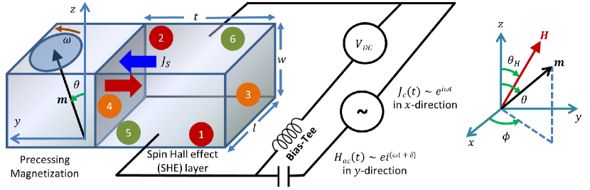
Figure 1: Schematic diagram of ST-FMR setup and axis assignments. With the help of a bias-tee, simultaneous ac transmission and dc voltage/current detection is possible in ST-FMR. A longitudinal ac current in $x$-direction $J_{c}$ across the surfaces marked by 1 and 2 of the SHE layer generates a transverse spin current density $J_{s}$ and it can drive the magnetization $\mathbf{m}$ into precession. $H$ is the applied dc magnetic field, $H_{ac}$ is the rf driving field produced from $J_{c}$ with a phase lag $\delta$, $\omega$ and $\theta$ are the precession frequency and angle, respectively. Spin potentials are developed across the surfaces marked by 3 and 4. Using a bias-tee, the dc voltage $V_{dc}$ can be detected and it comprises of both the contributions of longitudinal SMR and spin pumping due to ISHE. Also, charge potentials are developed across the surfaces marked by 5 and 6 due to transverse SMR. In the axis assignments, standard spherical coordinate system is used with azimuthal angle $\phi$ and polar angle $\theta$ for magnetization $\mathbf{m}$, and polar angle $\theta_{H}$ for the dc field $H$.

To develop the spin-circuit representation we can utilize the Ohm’s law with spin-orbit interaction (including both SHE and ISHE) Chen et al. (2013)

$$\left[{\begin{array}[]{c}\mathbf{J^{c}}\\ \mathbf{J^{z}}\\ \mathbf{J^{x}}\\ \mathbf{J^{y}}\\ \end{array}}\right]=\sigma\left[{\begin{array}[]{cccc}1&\theta_{sh}\mathbf{\hat{z}}\times&\theta_{sh}\mathbf{\hat{x}}\times&\theta_{sh}\mathbf{\hat{y}}\times\\ \theta_{sh}\mathbf{\hat{z}}\times&1&0&0\\ \theta_{sh}\mathbf{\hat{x}}\times&0&1&0\\ \theta_{sh}\mathbf{\hat{y}}\times&0&0&1\\ \end{array}}\right]\left[{\begin{array}[]{c}-\mathbf{\nabla}V^{c}\\ -\mathbf{\nabla}V^{z}\\ -\mathbf{\nabla}V^{x}\\ -\mathbf{\nabla}V^{y}\\ \end{array}}\right]$$

together with the charge and spin diffusion equations $\mathbf{\nabla\cdot J^{c}}=-\sigma\nabla^{2}V^{c}=0$ and $\mathbf{\nabla\cdot J^{x,y,z}}=-\sigma\nabla^{2}V^{x,y,z}=-(\sigma/\lambda^{2})V^{x,y,z}$, respectively, where $\mathbf{J^{c}}$ and $\mathbf{J^{x,y,z}}$ are current densities, and $V^{c}$ and $V^{x,y,z}$ are spin potentials, $\sigma$ is the conductivity, $\lambda$ is the spin diffusion length, and $\theta_{sh}$ is the spin Hall angle of the SHE layer.

Since we are not considering any charge component in the magnetic insulators, the generation of inverse spin Hall voltage is in the transverse direction due to the symmetry involved in the system, and unlike charge pumping, Brouwer (1998); *RefWorks:1324 a precessing magnet injects a pure spin current into surrounding conductors, Tserkovnyak, Brataas, and Bauer (2002a); *RefWorks:1041; Tserkovnyak et al. (2005) we consider a reduced 3-component version of the spin-circuit and show that it can reproduce the established expressions in literature for the dc voltage/current generated in ST-FMR experiments comprising both SMR and spin pumping. We further employ such formalism for multilayers like a spin-valve structure with an SHE layer sandwiched by two magnetic layers. Chen et al. (2013) We show how we can simply write a vector netlist comprising the conductances and voltage/current sources so that we can solve for the voltages/currents at the different nodes without invoking any boundary condition using a circuit solver. For complex structures, derivation of any analytical expression becomes tedious and this signifies the prowess of the spin-circuit approach.

Figure 2(a) shows the spin-circuit representation of ST-FMR that constitutes the spin-circuit representations of SHE layer, the charge current dependent spin current sources due to the charge to spin conversion in the SHE layer, and spin pumping. The instantaneous spin pumping can be represented by $\left[I_{sp}\right]=\left[G^{\uparrow\downarrow}\right]\left[V_{sp}\right]$, where $\left[V_{sp}\right]=(\hbar/2e)\,[0\;0\;1]^{T}$, $[G^{\uparrow\downarrow}]$ is the interfacial bare complex spin mixing conductance between the magnetic layer and the SHE layer represented in $(\mathbf{m},\mathbf{m^{\prime}},\mathbf{m}\times\mathbf{m^{\prime}})$ basis (where ^′ denotes the time derivative) as

$$\left[G^{\uparrow\downarrow}\right]=\left[\begin{array}[]{crr}0&0&0\\ 0&2G_{r}&2G_{i}\\ 0&-2G_{i}&2G_{r}\end{array}\right],$$ (1)

$\left[I_{sp}\right]=(\hbar/2e)\,[0\;2G_{i}\;2G_{r}]^{T}$ in $(\mathbf{m},\mathbf{m^{\prime}},\mathbf{m}\times\mathbf{m^{\prime}})$ basis, and $2G_{r(i)}$ is the real (imaginary) part of the bare complex spin mixing conductance $G^{\uparrow\downarrow}$. The bulk diffusion in the SHE layer can be represented by a $\pi$-circuit as shown in the Fig. 2(a) with $\left[G_{1(2)}\right]=G_{1(2)}\left[I_{3\times 3}\right]$, where $G_{1}=G_{\lambda}\mathrm{tanh}(t/2\lambda)$, $G_{2}=G_{\lambda}\mathrm{csch}(t/\lambda)$, $G_{\lambda}=\sigma lw/\lambda$, and $\left[I_{3\times 3}\right]$ is the ${3\times 3}$ identity matrix. The spin current sources in the Fig. 2(a) in $z$-$x$-$y$ basis can be written as

$$\left[I_{0,zxy}^{s}\right]=\beta G_{0}\left(V_{1}^{c}-V_{2}^{c}\right)\left[1\;0\;0\right]^{T}$$ (2)

where $G_{0}=\sigma tw/l$ and $\beta=\theta_{sh}l/t$. After converting to $(\mathbf{m},\mathbf{m^{\prime}},\mathbf{m}\times\mathbf{m^{\prime}})$ basis, the Equation (2) becomes (see supplementary material)

$$\left[I_{0}^{s}\right]=I_{0}^{s0}m_{z}\mathbf{m}+I_{0}^{s0}\frac{1}{\omega}\mathbf{m}\times\mathbf{m^{\prime}}$$ (3)

where $I_{0}^{s0}=\beta G_{0}\left(V_{1}^{c}-V_{2}^{c}\right)$.

Applying KCL at the nodes 3 and 4 in the spin-circuit shown in the Fig. 2(a), we get (see supplementary material)

$$\left[{\begin{array}[]{cc}\left[G_{1}\right]+\left[G_{2}\right]&-\left[G_{2}\right]\\ -\left[G_{2}\right]&\left[G_{1}\right]+\left[G_{2}\right]+\left[G^{\uparrow\downarrow}\right]\\ \end{array}}\right]\left[{\begin{array}[]{c}\left[V_{3}^{s}\right]\\ \left[V_{4}^{s}\right]\\ \end{array}}\right]=\left[{\begin{array}[]{c}-\left[I_{0}^{s}\right]\\ \left[I_{0}^{s}\right]+\left[I_{sp}\right]\\ \end{array}}\right].$$ (4)

Using the superposition principle in circuit theory, i.e., the contributions due to different voltage/current sources can be considered separately, we can determine the contributions due to SMR and spin pumping accordingly.

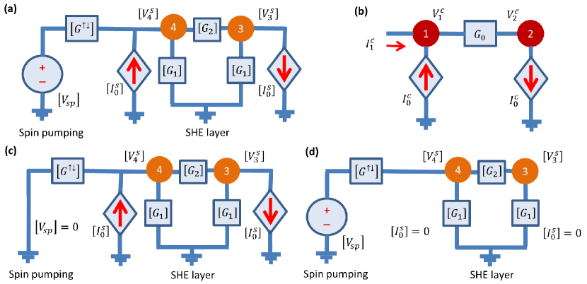
Figure 2: (a) Spin-circuit representation of ST-FMR. Spin potentials are developed at the surfaces marked by 3 and 4. $\left[I_{0}^{s}\right]$ is the charge current dependent spin current source due to SHE and $\left[V_{sp}\right]$ acts as the spin battery due to spin pumping. The bulk diffusion in the SHE layer can be represented by a $\pi$-circuit defined in the text. (b) The charge circuit for the spin-to-charge conversion by ISHE with the spin current dependent charge current sources $I_{0}^{c}$ with $G_{0}$ representing the conductance of the SHE layer. (c) Spin-circuit representation of ST-FMR without considering the spin battery $\left[V_{sp}\right]$. (d) Spin-circuit representation of ST-FMR without considering the spin current sources $\left[I_{0}^{s}\right]$.

Figure 2(b) shows the charge circuit counterpart comprising the spin current dependent charge current sources due to ISHE and the conductance $G_{0}$ of the SHE layer. A conductance in case the magnet is metallic can be included by putting the conductance in parallel to $G_{0}$ to account for the current shunting. Roy (2017a) The charge current sources in the Fig. 2(b) can be expressed as

$$I_{0}^{c}=\beta G_{0}\left(V_{3}^{z}-V_{4}^{z}\right).$$ (5)

Applying KCL at node 1 of the charge-circuit in Fig. 2(b), we get

$$I_{1}^{c}=-I_{0}^{c}+G_{0}\left(V_{1}^{c}-V_{2}^{c}\right).$$ (6)

The contribution due to SMR is given by the spin-circuit in the Fig. 2(c) as follows.

$$\left[{\begin{array}[]{cc}\left[G_{1}\right]+\left[G_{2}\right]&-\left[G_{2}\right]\\ -\left[G_{2}\right]&\left[G_{1}\right]+\left[G_{2}\right]+\left[G^{\uparrow\downarrow}\right]\\ \end{array}}\right]\left[{\begin{array}[]{c}\left[V_{3}^{s}\right]\\ \left[V_{4}^{s}\right]\\ \end{array}}\right]=\left[{\begin{array}[]{c}-\left[I_{0}^{s}\right]\\ \left[I_{0}^{s}\right]\\ \end{array}}\right].$$ (7)

After solving the above equations in the matrix form, we get

$$V_{3}^{m}-V_{4}^{m}=-\frac{2\,\mathrm{tanh}(t/2\lambda)}{G_{\lambda}}I_{0}^{s0}m_{z},$$ (8)

$$V_{3}^{m^{\prime}}-V_{4}^{m^{\prime}}=\frac{1}{G_{\lambda}}Im\{F(t)\}I_{0}^{s0}\frac{1}{\omega},$$ (9)

and

$$V_{3}^{m\times m^{\prime}}-V_{4}^{m\times m^{\prime}}=-\frac{\mathrm{tanh}(t/\lambda)}{G_{\lambda}}I_{0}^{s0}\frac{1}{\omega}$$

$$-\frac{(G_{\lambda}\mathrm{tanh}(t/\lambda)+2G_{r})\,\mathrm{tanh}^{2}(t/\lambda)\,\mathrm{tanh}^{2}(t/2\lambda)}{(G_{\lambda}\mathrm{tanh}(t/\lambda)+2G_{r})^{2}+4G_{i}^{2}}I_{0}^{s0}\frac{1}{\omega}$$ (10)

where

$$F(t)=\frac{(2G^{\uparrow\downarrow}/G_{\lambda})\,\mathrm{tanh}^{2}(t/2\lambda)}{1+(2G^{\uparrow\downarrow}/G_{\lambda})\,\mathrm{coth}(t/\lambda)}.$$ (11)

We can write the spin voltage differences in the longitudinal and transverse directions as follows (see supplementary material).

$$V_{3}^{z}-V_{4}^{z}=(V_{3}^{m}-V_{4}^{m})m_{z}+(V_{3}^{m\times m^{\prime}}-V_{4}^{m\times m^{\prime}})\left(1-m_{z}^{2}\right)\omega,$$ (12)

$$V_{3}^{x}-V_{4}^{x}= (V_{3}^{m}-V_{4}^{m})m_{x}-(V_{3}^{m^{\prime}}-V_{4}^{m^{\prime}})\,m_{y}\,\omega$$

$$-(V_{3}^{m\times m^{\prime}}-V_{4}^{m\times m^{\prime}})\,m_{z}m_{x}\,\omega.$$ (13)

From Equations (6) and (12), and using the equality $2\mathrm{tanh}(t/2\lambda)=\mathrm{tanh}(t/\lambda)\,(1+\mathrm{tanh}^{2}(t/2\lambda))$, we get

$$\frac{I_{1}^{c}}{tw}=\frac{\sigma}{l}\left(V_{1}^{c}-V_{2}^{c}\right) \left\{1+\theta_{SH}^{2}(\lambda/t)\left[2\mathrm{tanh}(t/2\lambda)\right.\right.$$

$$-\left.\left.(1-m_{z}^{2})\,Re\{F(t)\}\right]\right\}.$$ (14)

Using $I_{5}^{c}=\beta G_{0}\left(V_{3}^{x}-V_{4}^{x}\right)$ and Equation (13), we get

$$\frac{I_{5}^{c}}{lt}=-\theta_{SH}^{2}\frac{\sigma\lambda}{lt}\left(V_{1}^{c}-V_{2}^{c}\right)\left[m_{z}m_{x}\,Re+m_{y}\,Im\right]\,F(t).$$ (15)

The Equations (14) and (15) are known as longitudinal and transverse SMR, respectively and these results match the existing results in the literature. Chen et al. (2013); Hong, Sayed, and Datta (2016) Note that the SMR is proportional to the square of the spin Hall angle ($\theta_{sh}^{2}$) due to the coordinated action of SHE and ISHE, and therefore materials with higher values of $\theta_{sh}$ would aid in increasing the SMR.

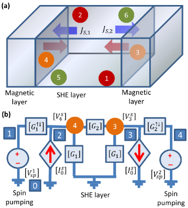
Figure 3: (a) A spin-valve structure employing SMR i.e., a trilayer with an SHE layer sandwiched by two magnetic insulator layers. The SMR will be dependent on the magnetization directions of the two magnetic layers. (b) The corresponding spin-circuit representation employing the two interfacial spin-mixing conductances $G_{1}^{\uparrow\downarrow}$ and $G_{2}^{\uparrow\downarrow}$. and two spin batteries $[V_{sp}^{1}]$ and $[V_{sp}^{2}]$. The spin-circuit representation of the SHE layer remains same as shown in the Fig. 2(a). Charge potentials are developed at the surfaces marked by 1 and 2, and marked by 5 and 6 and the charge-circuit as presented in the Fig. 2(b) remains same.

The contribution due to spin pumping is given by the spin-circuit in the Fig. 2(d) as follows.

$$\left[{\begin{array}[]{cc}\left[G_{1}\right]+\left[G_{2}\right]&-\left[G_{2}\right]\\ -\left[G_{2}\right]&\left[G_{1}\right]+\left[G_{2}\right]+\left[G^{\uparrow\downarrow}\right]\\ \end{array}}\right]\left[{\begin{array}[]{c}\left[V_{3}^{s}\right]\\ \left[V_{4}^{s}\right]\\ \end{array}}\right]=\left[{\begin{array}[]{c}0\\ \left[I_{sp}\right]\\ \end{array}}\right].$$ (16)

After solving the above equations in the matrix form, we get

$$\left.V_{3}^{m^{\prime}}-V_{4}^{m^{\prime}}\right|_{sp}=(\hbar/2e)Im\{\eta(t)\},$$ (17)

and

$$\left.V_{3}^{m\times m^{\prime}}-V_{4}^{m\times m^{\prime}}\right|_{sp}=(\hbar/2e)Re\{\eta(t)\}$$ (18)

where

$$\eta(t)=\frac{(2G^{\uparrow\downarrow}/G_{\lambda})\,\mathrm{tanh}(t/2\lambda)}{1+(2G^{\uparrow\downarrow}/G_{\lambda})\,\mathrm{coth}(t/\lambda)}.$$ (19)

Note that there is no contribution in the direction of $\mathbf{m}$ since we are not considering any spin-wave propagation or magnons. From Equation (5), we get

$$\left.\frac{I_{0}^{c}}{tw}\right|_{sp}=\frac{\hbar}{2e}\theta_{SH}\frac{\sigma}{t}\left[Re\{\eta(t)\}\left(\mathbf{m}\times\mathbf{m^{\prime}}\right)_{z}+Im\{\eta(t)\}\mathbf{m^{\prime}}_{z}\right],$$ (20)

which matches the mathematical expression derived in literature. Chiba, Bauer, and Takahashi (2014) Note that in the ST-FMR experiments, the longitudinal SMR and spin pumping contributions can be separated from the involved angular dependence.

For a more complex system e.g., a spin-valve employing SMR Chen et al. (2013) as shown in the Fig. 3, the analytical expressions become tedious and this clearly signifies the prowess of the spin-circuit approach. We can simply write a netlist [see the node numbers in squares in the Fig. 3(b)] as follows and solve that using a circuit solver.

⬇

conductances = [1 2 $G_{1}^{\uparrow\downarrow}$; 3 4 $G_{2}^{\uparrow\downarrow}$;

2 0 $[G_{1}]$; 2 3 $[G_{2}]$; 3 0 $[G_{1}]$];

voltageSources = [1 0 $[V_{sp}^{1}]$; 4 0 $[V_{sp}^{2}]$];

currentSources = [0 2 $[I_{0}^{s}]$; 3 0 $[I_{0}^{s}]$];

While using a circuit solver, there is also the other way that we can follow i.e., convert $G_{1}^{\uparrow\downarrow}$ and $G_{2}^{\uparrow\downarrow}$ to $z$-$x$-$y$ basis, but mathematically working with the $z$-$x$-$y$ basis is tedious and therefore is not followed for the derivation of analytical expressions here.

To summarize, we have developed the spin-circuit representation of ST-FMR and have shown that both the SMR and spin pumping contributions match the established mathematical expressions in literature. Such circuits when complex can be simply solved using a circuit solver and therefore helps in analysis, benchmarking experimental results, and proposing creative designs of functional devices. We do need to consider the interfacial spin memory loss, Roy (2020); Gupta et al. (2020); Flores et al. (2020); Dolui and Nikolić (2017); Belashchenko, Kovalev, and van Schilfgaarde (2016); Rojas-Sánchez et al. (2014) which lowers the conductivity. Recent calculations Roy (2020, 2017b, 2018); Tao et al. (2018); Yu et al. (2018); Berger et al. (2018) signify the Elliott-Yafet spin relaxation mechanism in heavy metals for which $\lambda$ is dependent on thickness as conductivity varies with thickness of the samples. ST-FMR can allow us to understand and estimate the relevant parameters in the system and such understandings can benefit the device design using SHE, Roy (2014); Ramaswamy et al. (2018) which has potential for building future spintronic devices, alongwith other promising energy-efficient emerging devices. Roy (2016)

See the supplementary material for detailed derivation.

This work was supported by Science and Engineering Research Board (SERB) of India via sanction order SRG/2019/002166.

The data that support the findings of this study are available from the corresponding author upon reasonable request.

References

- Silsbee, Janossy, and Monod (1979) R. H. Silsbee, A. Janossy, and P. Monod, Phys. Rev. B 19, 4382 (1979).
- Heinrich et al. (1987) B. Heinrich, K. B. Urquhart, A. S. Arrott, J. F. Cochran, K. Myrtle, and S. T. Purcell, Phys. Rev. Lett. 59, 1756 (1987).
- Guan et al. (2007) Y. Guan, W. E. Bailey, E. Vescovo, C.-C. Kao, and D. A. Arena, J. Magn. Magn. Mater. 312, 374 (2007).
- Wang, Ramaswamy, and Yang (2018) Y. Wang, R. Ramaswamy, and H. Yang, J. Phys. D: Appl. Phys 51, 273002 (2018).
- Landau and Lifshitz (1935) L. Landau and E. Lifshitz, Phys. Z. Sowjet. 8, 153 (1935).
- Gilbert (2004) T. L. Gilbert, IEEE Trans. Magn. 40, 3443 (2004).
- Dyakonov and Perel (1971) M. I. Dyakonov and V. I. Perel, Sov. Phys. JETP Lett. 13, 467 (1971).
- Hirsch (1999) J. E. Hirsch, Phys. Rev. Lett. 83, 1834 (1999).
- Zhang (2000) S. Zhang, Phys. Rev. Lett. 85, 393 (2000).
- Murakami, Nagaosa, and Zhang (2003) S. Murakami, N. Nagaosa, and S. C. Zhang, Science 301, 1348 (2003).
- Sinova et al. (2004) J. Sinova, D. Culcer, Q. Niu, N. A. Sinitsyn, T. Jungwirth, and A. H. MacDonald, Phys. Rev. Lett. 92, 126603 (2004).
- Sinova et al. (2015) J. Sinova, S. O. Valenzuela, J. Wunderlich, C. H. Back, and T. Jungwirth, Rev. Mod. Phys. 87, 1213 (2015).
- Valenzuela and Tinkham (2006) S. O. Valenzuela and M. Tinkham, Nature 442, 176 (2006).
- Roy (2014) K. Roy, J. Phys. D: Appl. Phys. 47, 422001 (2014).
- Wang et al. (2006) X. Wang, G. E. W. Bauer, B. J. van Wees, A. Brataas, and Y. Tserkovnyak, Phys. Rev. Lett. 97, 216602 (2006).
- Jiao and Bauer (2013) H. Jiao and G. E. W. Bauer, Phys. Rev. Lett. 110, 217602 (2013).
- Azevedo et al. (2005) A. Azevedo, L. H. Vilela-Leão, R. L. Rodríguez-Suárez, A. B. Oliveira, and S. M. Rezende, J. Appl. Phys. 97, 10C715 (2005).
- Saitoh et al. (2006) E. Saitoh, M. Ueda, H. Miyajima, and G. Tatara, Appl. Phys. Lett. 88, 182509 (2006).
- Tserkovnyak, Brataas, and Bauer (2002a) Y. Tserkovnyak, A. Brataas, and G. E. W. Bauer, Phys. Rev. Lett. 88, 117601 (2002a).
- Tserkovnyak, Brataas, and Bauer (2002b) Y. Tserkovnyak, A. Brataas, and G. E. W. Bauer, Phys. Rev. B 66, 224403 (2002b).
- Tserkovnyak et al. (2005) Y. Tserkovnyak, A. Brataas, G. E. W. Bauer, and B. I. Halperin, Rev. Mod. Phys. 77, 1375 (2005).
- Brataas et al. (2012) A. Brataas, Y. Tserkovnyak, G. E. W. Bauer, and P. J. Kelly, “Spin pumping and spin transfer,” in Spin Current, Vol. 17, edited by S. Maekawa, S. O. Valenzuela, E. Saitoh, and T. Kimura (Oxford University Press, 2012) pp. 87–135.
- Slonczewski (1996) J. C. Slonczewski, J. Magn. Magn. Mater. 159, L1 (1996).
- Berger (1996) L. Berger, Phys. Rev. B 54, 9353 (1996).
- Onsager (1931a) L. Onsager, Phys. Rev. 37, 405 (1931a).
- Onsager (1931b) L. Onsager, Phys. Rev. 38, 2265 (1931b).
- Liu et al. (2011) L. Liu, T. Moriyama, D. C. Ralph, and R. A. Buhrman, Phys. Rev. Lett. 106, 036601 (2011).
- Wang et al. (2014) Y. Wang, P. Deorani, X. Qiu, J. H. Kwon, and H. Yang, Appl. Phys. Lett. 105, 152412 (2014).
- Zhang et al. (2015) W. Zhang, W. Han, X. Jiang, S. H. Yang, and S. S. P. Parkin, Nature Phys. 11, 496 (2015).
- Jungfleisch et al. (2017) M. B. Jungfleisch, J. Ding, W.Zhang, W. Jiang, J. E. Pearson, V. Novosad, and A. Hoffmann, Nano Lett. 17, 8 (2017).
- Chen et al. (2013) Y. T. Chen, S. Takahashi, H. Nakayama, M. Althammer, S. T. B. Goennenwein, E. Saitoh, and G. E. W. Bauer, Phys. Rev. B 87, 144411 (2013).
- Nakayama et al. (2013) H. Nakayama, M. Althammer, Y. T. Chen, K. Uchida, Y. Kajiwara, D. Kikuchi, T. Ohtani, S. Geprägs, M. Opel, S. Takahashi, R. Gross, G. E. W. Bauer, S. T. B. Goennenwein, and E. Saitoh, Phys. Rev. Lett. 110, 206601 (2013).
- Chiba, Bauer, and Takahashi (2014) T. Chiba, G. E. W. Bauer, and S. Takahashi, Phys. Rev. Appl. 2, 034003 (2014).
- Chiba et al. (2015) T. Chiba, M. Schreier, G. E. W. Bauer, and S. Takahashi, J. Appl. Phys. 117, 17C715 (2015).
- Schreier et al. (2015) M. Schreier, T. Chiba, A. Niedermayr, J. Lotze, H. Huebl, S. Geprägs, S. Takahashi, G. E. W. Bauer, R. Gross, and S. T. B. Goennenwein, Phys. Rev. B 92, 144411 (2015).
- Jungfleisch et al. (2015) M. B. Jungfleisch, A. V. Chumak, A. Kehlberger, V. Lauer, D. H. Kim, M. C. Onbasli, C. A. Ross, M. Kläui, and B. Hillebrands, Phys. Rev. B 91, 134407 (2015).
- Sklenar et al. (2015) J. Sklenar, W. Zhang, M. B. Jungfleisch, W. Jiang, H. Chang, J. E. Pearson, M. Wu, J. B. Ketterson, and A. Hoffmann, Phys. Rev. B 92, 174406 (2015).
- Thomson (1856) W. Thomson, Philos. Trans. R. Soc. London 146, 649 (1856).
- Baibich et al. (1988) M. N. Baibich, J. M. Broto, A. Fert, F. NguyenVanDau, F. Petroff, P. Etienne, G. Creuzet, A. Friederich, and J. Chazelas, Phys. Rev. Lett. 61, 2472 (1988).
- Binasch et al. (1989) G. Binasch, P. Grünberg, F. Saurenbach, and W. Zinn, Phys. Rev. B 39, 4828 (1989).
- Julliere (1975) M. Julliere, Phys. Lett. A 54, 225 (1975).
- Butler et al. (2001) W. H. Butler, X. G. Zhang, T. C. Schulthess, and J. M. MacLaren, Phys. Rev. B 63, 054416 (2001).
- Parkin et al. (2004) S. S. P. Parkin, C. Kaiser, A. Panchula, P. M. Rice, B. Hughes, M. G. Samant, and S. H. Yang, Nature Mater. 3, 862 (2004).
- Yuasa et al. (2004) S. Yuasa, T. Nagahama, A. Fukushima, Y. Suzuki, and K. Ando, Nature Mater. 3, 868 (2004).
- Rabaey, Chandrakasan, and Nikoliç (2003) J. M. Rabaey, A. P. Chandrakasan, and B. Nikoliç, Digital Integrated Circuits (Pearson Education, 2003).
- (46) HSPICE, Circuit simulation software, Synopsys, www.synopsys.com.
- Sah (1971) C.-T. Sah, Phys. Stat. Sol. (a) 7, 541 (1971).
- Brataas, Bauer, and Kelly (2006) A. Brataas, G. E. W. Bauer, and P. J. Kelly, Phys. Rep. 427, 157 (2006).
- Srinivasan et al. (2014) S. Srinivasan, V. Diep, B. Behin-Aein, A. Sarkar, and S. Datta, “Modeling multi-magnet networks interacting via spin currents,” in Handbook of Spintronics, edited by Y. Xu, D. D. Awschalom, and J. Nitta (Springer Netherlands, Dordrecht, 2014) pp. 1–49.
- Hong, Sayed, and Datta (2016) S. Hong, S. Sayed, and S. Datta, IEEE Trans. Nanotech. 15, 225 (2016).
- Roy (2017a) K. Roy, Phys. Rev. Appl. (Lett.) 8, 011001 (2017a).
- Brouwer (1998) P. W. Brouwer, Phys. Rev. B 58, R10135 (1998).
- Büttiker, Thomas, and Prêtre (1994) M. Büttiker, H. Thomas, and A. Prêtre, Z. Phys. B 94, 133 (1994).
- Roy (2020) K. Roy, Appl. Phys. Lett. 117, 022404 (2020).
- Gupta et al. (2020) K. Gupta, R. J. H. Wesselink, R. Liu, Z. Yuan, and P. J. Kelly, Phys. Rev. Lett. 124, 087702 (2020).
- Flores et al. (2020) G. G. B. Flores, A. A. Kovalev, M. van Schilfgaarde, and K. D. Belashchenko, Phys. Rev. B 101, 224405 (2020).
- Dolui and Nikolić (2017) K. Dolui and B. K. Nikolić, Phys. Rev. B 96, 220403 (2017).
- Belashchenko, Kovalev, and van Schilfgaarde (2016) K. D. Belashchenko, A. A. Kovalev, and M. van Schilfgaarde, Phys. Rev. Lett. 117, 207204 (2016).
- Rojas-Sánchez et al. (2014) J. C. Rojas-Sánchez, N. Reyren, P. Laczkowski, W. Savero, J. P. Attané, C. Deranlot, M. Jamet, J. M. George, L. Vila, and H. Jaffrès, Phys. Rev. Lett. 112, 106602 (2014).
- Roy (2017b) K. Roy, Phys. Rev. B 96, 174432 (2017b).
- Roy (2018) K. Roy, Proc. SPIE Nanoscience (Spintronics XI) 10732, 1073207 (2018).
- Tao et al. (2018) X. Tao, Q. Liu, B. Miao, R. Yu, Z. Feng, L. Sun, B. You, J. Du, K. Chen, S. Zhang, L. Zhang, Z. Yuan, D. Wu, and H. Ding, Sci. Adv. 4, eaat1670 (2018).
- Yu et al. (2018) R. Yu, B. F. Miao, L. Sun, Q. Liu, J. Du, P. Omelchenko, B. Heinrich, M. Wu, and H. F. Ding, Phys. Rev. Mater. 2, 074406 (2018).
- Berger et al. (2018) A. J. Berger, E. R. J. Edwards, H. T. Nembach, O. Karis, M. Weiler, and T. J. Silva, Phys. Rev. B 98, 024402 (2018).
- Ramaswamy et al. (2018) R. Ramaswamy, J. M. Lee, K. Cai, and H. Yang, Appl. Phys. Rev. 5, 031107 (2018).
- Roy (2016) K. Roy, SPIN 6, 1630001 (2016).