Generalizable control for multiparameter quantum metrology

Abstract

Quantum control can be employed in quantum metrology to improve the precision limit for the estimation of unknown parameters. The optimal control, however, typically depends on the actual values of the parameters and thus needs to be designed adaptively with the updated estimations of those parameters. Traditional methods, such as gradient ascent pulse engineering (GRAPE), need to be rerun for each new set of parameters encountered, making the optimization costly, especially when many parameters are involved. Here we study the generalizability of optimal control, namely, optimal controls that can be systematically updated across a range of parameters with minimal cost. In cases where control channels can completely reverse the shift in the Hamiltonian due to a change in parameters, we provide an analytical method which efficiently generates optimal controls for any parameter starting from an initial optimal control found by either GRAPE or reinforcement learning. When the control channels are restricted, the analytical scheme is invalid, but reinforcement learning still retains a level of generalizability, albeit in a narrower range. In cases where the shift in the Hamiltonian is impossible to decompose to available control channels, no generalizability is found for either the reinforcement learning or the analytical scheme. We argue that the generalization of reinforcement learning is through a mechanism similar to the analytical scheme. Our results provide insights into when and how the optimal control in multiparameter quantum metrology can be generalized, thereby facilitating efficient implementation of optimal quantum estimation of multiple parameters, particularly for an ensemble of systems with ranges of parameters.

I Introduction

One of the main goals of quantum metrology is to identify the highest possible precision for the estimation of unknown parameters and find practical ways to approach that limit. There have been extensive studies on the optimization of probe states and measurements to achieve better precisions Humphreys et al. (2013); Pezzè et al. (2017); Yue et al. (2014); Yuan and Fung (2017). Recently, it was realized that quantum control during the evolution can be optimized to improve the precision in the estimation of a single parameter Yuan and Fung (2015); Liu and Yuan (2017a); Pang and Jordan (2017); Fraïsse and Braun (2017); Fiderer et al. (2019); Haine and Hope (2020) or multiple parameters Yuan (2016); Liu and Yuan (2017b). Numerical methods such as gradient ascent pulse engineering (GRAPE) have been employed to obtain optimal controls Khaneja et al. (2005); Liu and Yuan (2017a, b). The optimal controls, however, typically depend on the values of the parameters, which need to be adaptively updated with the accumulation of measurement data. In this process, one typically starts with a nominal (or assumed) value of the unknown parameter, finds the control optimal for that nominal value, and performs a measurement using that optimized control. This measurement gives an estimated value of the unknown parameter, along with an accuracy which should fall in a certain theoretical limit dependent on the control process. Then, if one is not satisfied with this theoretical limit, the process is repeated with a new control optimized at the last estimated value until a certain convergence criterion is met. For an ensemble of systems with parameters to be estimated, varying in a range, such optimization has to be repeated many times, making it resource consuming and cumbersome [see Fig. 1(a)]. A method that can systematically update optimal controls across a range of parameters with minimal cost, a characteristic termed generalizability, is then desirable, particularly for the estimation of multiple parameters as the search space becomes much larger, and performing a brand-new search of optimal controls for each set of parameters could become prohibitively expensive.

Reinforcement learning (RL) is an alternative method that can be used to estimate multiple parameters. The main idea of RL is to convert an optimization problem into a game, with the goals and constraints of the problem encapsulated as rules in the game. A computer agent, through playing the game in an emulator, obtains rewards depending on its performance. A procedure that maximizes rewards therefore leads to an optimized solution of the desired problem. Reinforcement learning has demonstrated its superior power in playing several types of games Mnih et al. (2013, 2015); Silver et al. (2016). It has also been shown to improve solutions to many problems in quantum information science Fösel et al. (2018), quantum control Bukov et al. (2018); Niu et al. (2019); Zhang et al. (2019); Lin et al. (2020), and in particular quantum metrology Xu et al. (2019); Schuff et al. (2020); Fiderer et al. (2021). In a previous work on the single-parameter quantum estimation, we have shown that RL has an important advantage: the generalizability Xu et al. (2019). An agent trained for one value of the parameter can be straightforwardly generalized to other values of the parameter, producing near-optimal controls [see Fig. 1(b)]. This makes RL efficient for quantum estimation with an ensemble of systems where the values of the parameter may vary within a certain range.

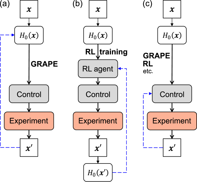
Figure 1: Illustrative flowcharts for estimating $\bm{x}$, a vector encapsulating all parameters to be estimated, using controls optimized by (a) GRAPE, (b) RL, and (c) the analytical scheme. In all panels, the blue dashed line indicates that subsequent control should be optimized according to updated estimations of the parameters of the previous step. In (a), GRAPE has to be rerun whenever an updated estimation of the parameters is encountered. In (b), the training of the RL agent is only conducted once and controls for updated parameters can be generated directly from the agent without additional training. In (c), while the initial optimal control has to be found by either GRAPE or RL, subsequent updates can be efficiently done according to Theorem 1.

The generalizability afforded by RL Sutton and Barto (2018) has been actively studied in the literature Tobin et al. (2017); Lee et al. (2020). While a complete understanding of its origin is still lacking, the present consensus is that the generalizability likely arises from the fact that an RL agent underfits the training data sut ; Cobbe et al. (2019); Sutton and Barto (2018). Recently, several schemes have been designed to quantify the generalization in RL Cobbe et al. (2019); Zhang et al. (2018); Packer et al. (2019), and it has been found that techniques such as domain randomization Tobin et al. (2017), network randomization Lee et al. (2020) and the prediction model Pathak et al. (2017) could improve the generalizability. In quantum parameter estimation, the updated estimations of parameters correspond to the updated environments in RL. Here the generalization of RL is essentially a problem of training an RL agent that works for an ensemble of systems with ranges of unknown parameters, as we have done in this work.

The main goal of this paper is to elucidate how the generalizability is maintained in the situation of multiparameter quantum estimation. To this purpose, we introduce an analytical method which adjusts the controls (already optimal for certain parameters) to reverse the shift of the Hamiltonian stemming from the change of the parameters so as to maintain the optimality [see Fig. 1(c)]. This analytical method only applies to the situation in which the controls are “complete,” i.e., there are sufficient control channels to absorb the shift in the Hamiltonian. In this situation, generalization using the analytical method is most effective as only the initial control for a chosen set of parameters needs to be found by RL or GRAPE. When the shift in the Hamiltonian due to a change in parameters can only be partially absorbed into available control channels, the analytical method is no longer valid. However, RL still provides generalizable optimal control, albeit for a narrower range of parameters, and we believe that the mechanism for the generalizability afforded by RL is similar to the analytical scheme. Finally, if the shift in the Hamiltonian cannot be decomposed into available control channels, such as the coupling between two spins considered in this paper, neither RL nor the analytical method provides any generalizability. In this case, one has to rerun either RL or GRAPE for each new set of parameters. Our results provide insights into when and how the optimal control in multiparameter quantum metrology can be generalized, thereby facilitating efficient implementation of optimal quantum estimation of multiple parameters, particularly for an ensemble of systems with ranges of parameters.

The remainder of the paper is organized as follows. In Sec. II we briefly review the theory on multiparameter estimation and present the two examples considered in this paper. Section III explains the methods used in this work, including GRAPE, RL, and the analytical scheme. In Sec. IV we show detailed results on the generalizability applied to the two examples. We summarize in Sec. V. Necessary details on the implementation of RL, the comparison between RL and GRAPE, and additional discussion about the generalizability are provided in the Appendixes.

II multiparameter quantum estimation

We consider the time evolution of a quantum state described by the master equation Breuer and Petruccione (2002)

$$\partial_{t}\rho(t)=\mathcal{L}[\rho(t)],$$ (1)

where $\mathcal{L}[\rho(t)]=-i[H,\rho(t)]+{\color[rgb]{0,0,0}\Gamma[\rho(t)]}$. ${\color[rgb]{0,0,0}\Gamma[\rho(t)]}$ describes the effect of noises and $H$ is the Hamiltonian that can be decomposed as

$$H=H_{0}(\bm{x})+\sum_{i=1}^{P}u_{i}(t)H_{i},$$ (2)

where $H_{0}(\bm{x})$ is the free evolution with $\bm{x}$, a vector encapsulating the unknown parameters of interest. The term $u_{i}(t)H_{i}$ represents the control Khaneja et al. (2005) and $P$ is the number of available control channels. We discretize the total evolution time $T$ into $N=T/\Delta t$ equal time slices, and a piecewise constant pulse sequence generates an evolution as

$$\rho(T)=\prod_{j=0}^{N-1}e^{\Delta t\mathcal{L}_{j}}\rho(0),$$ (3)

where $\mathcal{L}_{j}$ is the superoperator for the $j$th time slice. The control field is described by the sequence of $u_{i}(j\Delta t)$ on the interval $[0,T]$.

Given a positive-operator-valued measurement (POVM) $\quantity{\Pi_{y}}$, the covariance matrix of the measurements is lower bounded by Liu et al. (2020)

$$\operatorname{\mathrm{cov}}(\widehat{\bm{x}},\Pi_{y})\geqslant\frac{1}{n}\mathcal{F}_{\mathrm{cl}}^{-1}(\Pi_{y})\geqslant\frac{1}{n}\mathcal{F}^{-1},$$ (4)

where $\widehat{\bm{x}}$ is the unbiased estimator of $\bm{x}$ and $n$ is the number of repetitions. The first inequality is the Cramér-Rao bound, where $\operatorname{\mathcal{F}_{\mathrm{cl}}}(\Pi_{y})$ is the classical Fisher information matrix which depends on the choice of the measurement,

$$\mathcal{F}_{\mathrm{cl},\alpha\beta}=\sum_{y}\frac{\partial_{\bm{x}_{\alpha}}p_{y|\bm{x}}\partial_{\bm{x}_{\beta}}p_{y|\bm{x}}}{p_{y|\bm{x}}},$$ (5)

where $p_{y|\bm{x}}=\tr[\rho(t)\Pi_{y}]$. The second inequality is the quantum Cramér-Rao bound with $\mathcal{F}$ the quantum Fisher information matrix, which typically cannot be attained for the estimation of multiple parameters Liu et al. (2020). In this work we focus on the classical Cramér-Rao (CR) bound and take the trace of the covariance matrix as the figure of merit

$$|\delta\widehat{\bm{x}}|^{2}=\tr\operatorname{\mathrm{cov}}(\widehat{\bm{x}})\geqslant\operatorname{\tr\mathcal{F}_{\mathrm{cl}}^{-1}},$$ (6)

where $\Pi_{y}$ is omitted from the covariance matrix since a fixed POVM is used for each example and $\operatorname{\tr\mathcal{F}_{\mathrm{cl}}^{-1}}$ is the key quantity governing the precision of measurements that will be frequently referred to simply as the CR bound in the remainder of the paper.

In the following, we discuss the quantum parameter estimation under local controls on each qubit in the multiple-qubit system. The control Hamiltonian for $m$ qubits is

$$H_{c}(t)=\sum_{i=1}^{m}\bm{u}^{(i)}(t)\cdot\bm{\sigma}^{(i)},$$ (7)

where ${\bm{\sigma}}^{(i)}=(\sigma_{x}^{(i)},\sigma_{y}^{(i)},\sigma_{z}^{(i)})$ and $\sigma_{a}^{(i)}\equiv\mathbb{I}^{(1)}\otimes\cdots{\color[rgb]{0,0,0}\otimes}\mathbb{I}^{(i-1)}\otimes\sigma_{a}\otimes\mathbb{I}^{(i+1)}\otimes\cdots\otimes\mathbb{I}^{(m)}$. $\mathbb{I}$ is the $2\times 2$ identity matrix and $a=x,y,z$. The total number of control channels is $P=3m$. To compare with the optimal controls obtained with GRAPE, we will use the same examples studied in the previous work Liu and Yuan (2017b).

Example 1. The first example involves a two-qubit system where one qubit is in a magnetic field with both the magnitude and direction unknown. The other qubit acts as an ancillary qubit. The Hamiltonian of the first qubit is

$$H_{0}=\bm{B}\cdot\bm{\sigma}^{(1)},$$ (8)

where $\bm{B}=(B\sin\vartheta\cos\varphi,B\sin\vartheta\sin\varphi,B\cos\vartheta)$. The parameters to be estimated are $\bm{x}=(B,\vartheta,\varphi)$ characterizing the strength and direction of the magnetic field. The dephasing on the first qubit can be described by the Lindblad form,

$${\color[rgb]{0,0,0}\Gamma[\rho(t)]}=\frac{\gamma}{2}[\sigma_{z}^{(1)}\rho(t)\sigma_{z}^{(1)}-\rho(t)],$$ (9)

where $\gamma$ is the dephasing rate, which is set as $\gamma=0.2$ in our simulation. Different values of the dephasing rates are considered in Appendix D for comparison. We use the maximally entangled state $(\ket{00}+\ket{11})/\sqrt{2}$ as the probe state, and choose the projective measurement on the Bell bases $(\ket{00}\pm\ket{11})/\sqrt{2}$ and $(\ket{01}\pm\ket{10})/\sqrt{2}$.

Example 2. The second example is a $ZZ$-coupled two-qubit system. The Hamiltonian of the free evolution is

$$H_{0}=\omega_{1}\sigma^{(1)}_{z}+\omega_{2}\sigma^{(2)}_{z}+g\sigma^{(1)}_{z}\sigma^{(2)}_{z},$$ (10)

where $\bm{x}=(\omega_{1},\omega_{2},g)$ are the parameters to be estimated. Here $\omega_{1}$ and $\omega_{2}$ are individual magnetic fields along the $z$ direction, while $g$ is the $ZZ$-coupling strength. Both qubits suffer from dephasing dynamics

$$\Gamma[\rho(t)]=\sum_{i=1,2}\frac{\gamma_{i}}{2}[\sigma^{(i)}_{z}\rho(t)\sigma^{(i)}_{z}-\rho(t)],$$ (11)

where we set the dephasing rates $\gamma_{1}=\gamma_{2}=0.1$ in this work. Other values of the dephasing rates are studied in Appendix D. Under unitary dynamics (i.e., without noise), the optimal probe state for this system is $\ket{++}=(\ket{00}+\ket{01}+\ket{10}+\ket{11})/2$. We thus use $\ket{++}$ as the probe and the local measurements $\outerproduct{++}{++},\outerproduct{+-}{+-},\outerproduct{-+}{-+}$, and $\outerproduct{--}{--}$, where $\ket{\pm}=(\ket{0}\pm\ket{1})/\sqrt{2}$.

To facilitate the discussion, all parameters in this paper are considered dimensionless unless indicated otherwise, e.g., $B$, $\omega_{1}$, $\omega_{2}$, and $g$. The control fields are measured in the energy unit of 1 and the time $t$ is evaluated in the time unit of 1.

III Methods

III.1 Gradient ascent pulse engineering

For the case with only two parameters, Eq. (6) reduces to $\absolutevalue{\delta\widehat{\bm{x}}}^{2}\geqslant\det\operatorname{\mathcal{F}_{\mathrm{cl}}}/\tr\operatorname{\mathcal{F}_{\mathrm{cl}}}$. It is possible to derive the gradient of the CR bound with respect to the control field and perform GRAPE to find appropriate optimal controls Liu and Yuan (2017b). However, for the cases with more than two parameters, like the two examples above, taking the gradient of $\operatorname{\tr\mathcal{F}_{\mathrm{cl}}^{-1}}$ is not straightforward. Reference Liu and Yuan (2017b) introduced another objective function $f_{0}(T)$ as

$$f_{0}(T)^{-1}=\sum_{\alpha}\frac{1}{\mathcal{F}_{\mathrm{cl},\alpha\alpha}(T)},$$ (12)

which provides a lower bound to $\operatorname{\tr\mathcal{F}_{\mathrm{cl}}^{-1}}$ since $\quantity[\operatorname{\mathcal{F}_{\mathrm{cl}}^{-1}}]_{\alpha\alpha}\geqslant 1/\mathcal{F}_{\mathrm{cl},\alpha\alpha}$ and $\operatorname{\tr\mathcal{F}_{\mathrm{cl}}^{-1}}\geqslant\sum_{\alpha}1/\mathcal{F}_{\mathrm{cl},\alpha\alpha}$. Practically, the optimal controls are found by optimizing $f_{0}(T)$, even though it is not necessarily the optimization of the desired CR bound $\operatorname{\tr\mathcal{F}_{\mathrm{cl}}^{-1}}$. While we largely follows Ref. Liu and Yuan (2017b) to repeat the results obtained with GRAPE, we additionally apply the steepest gradient ascent method Ruder (2016) and the Adam method Kingma and Ba (2014) to update the control field, which are numerically more efficient than the simple updating scheme employed in Ref. Liu and Yuan (2017b).

The evolution of the density matrix must be evaluated $N^{2}$ times to compute the gradient with respect to control, while there are $N$ piecewise controls that need to be updated Xu et al. (2019). Though the time complexity of GRAPE can be reduced from $O{(N^{3})}$ to $O{(N^{2})}$ by spending more computer memory on storing the superoperators, the GRAPE method, as can be seen in Sec. IV, quickly becomes prohibitively expensive as the size of the problem increases.

III.2 Reinforcement learning

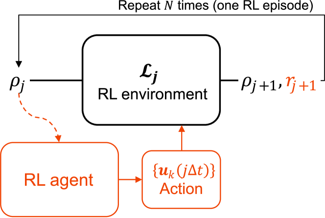
Figure 2: Schematics of the reinforcement learning framework. At the $j$th time step, the RL agent observes the current state as the density matrix $\rho_{j}\equiv\rho(j\Delta t)$ and takes an action as the control on the system. As a consequence, the state evolves to a new one at the $(j+1)$th time step while the agent receives an immediate reward. After completing one episode, the state is reset to the probe state.

For the piecewise control in Eq. (3), we can interpret the optimization problem as a Markov decision process in RL. Figure 2 shows the schematics of RL. The RL procedure is essentially an interaction between an agent and its environment, the latter of which involves a state space $\mathcal{S}$, an action space $\mathcal{A}$, and a numerical reward $\mathcal{R}$ Sutton and Barto (2018). The behavior of the agent is defined by a policy. In this work we use the deterministic policy, namely, it always maps $s_{j}\in\mathcal{S}$ to a specific action $a_{j}\in\mathcal{A}$ sil . At each time step $j$, the agent observes the current state $s_{j}$ and chooses an action $a_{j}\in\mathcal{A}$ according to its policy. The action $a_{j}$ constitutes the control $\bm{u}(j\Delta t)$ which steers the quantum state according to the dynamics of the environment described by the time evolution (1), while the agent receives an immediate reward $r_{j+1}$. The agent then observes the state $s_{j+1}$ and conducts action $a_{j+1}$ prescribed by the environment. This procedure is iterated until the target time $T$ (or total number of steps $N$) is reached, concluding one episode of RL. Each episode is summarized by a trajectory of states, actions, and rewards as $\quantity(s_{0},a_{0},r_{1},s_{1},\dots,a_{N-1},r_{N},s_{N})$. A replay memory is used to store $(s_{j},a_{j},r_{j+1},s_{j+1})$ (refered to as a sample) at each time step in the iteration. The RL agent is then trained using samples from the replay memory, which stabilizes the learning process Lin (1993); Mnih et al. (2013).

Since the action $a_{j}$ influences not only the immediate reward $r_{j+1}$ but also the future rewards $r_{k>j+1}$, the immediate reward alone is not an appropriate objective for training the RL agent. To take into account the future rewards, we define the total discounted reward $R_{j}=\sum_{k=j}^{N}\alpha^{k-j}_{\rm rl}r_{k+1}$ with $\alpha_{\rm rl}\in[0,1)$ the discount rate Sutton and Barto (2018). In practice, noises must be added to the actions chosen so as to prevent the simulation being trapped in a local minimum sil ; Lillicrap et al. (2015). Therefore, $R_{j}$ can have different values across different episodes, depending on the policy and the dynamics of the environment. We therefore use the expectation value $R_{j}$ across all episodes associated with the given deterministic policy and dynamics, $\mathbb{E}\quantity[R_{j}]$, as our objective. Practically, the RL agent maximizes the expected value of the total discounted reward at the initial state, $\mathbb{E}\quantity[R_{0}]$ Sutton and Barto (2018).

In this work we assume that the density matrix $\rho(j\Delta t)$ of any quantum state concerned is fully known to the agent Fösel et al. (2018); Xu et al. (2019); Schuff et al. (2020), which may not be true in experiments Leonhardt (1997); James et al. (2001). Our numerical simulation can be viewed as an emulator with regard to the RL procedure. In our numerical simulation, we must guess a value of the parameter to build the emulator for the RL agent. During one episode (either training or testing) of RL, the master equation is evaluated $N$ times in the RL environment. The time complexity for each episode is therefore $O{(N)}$. For a given problem, the training may actually be slower than GRAPE as a large prefactor is added depending on the details of the algorithm. Nevertheless, the generalizability afforded by RL can be advantageous in certain situations.

We employ the deep deterministic policy gradient (DDPG) reinforcement learning algorithm Lillicrap et al. (2015), which uses neural networks as function approximators of the agent. The agent’s policy is chosen to be deterministic for the following reasons. First, it can treat continuous actions as required in our problems. Second, computing the deterministic policy requires fewer samples than otherwise sil , which saves computational resources. Third, the main subject of our study is the generalizability, and having deterministic policies greatly facilitates evaluating the generalization of RL. The implementation of the DDPG procedure is detailed in Appendix A.

III.3 Analytical scheme

We now introduce the method of adjusting the optimal controls obtained for the parameters $\bm{x}$ to the new one $\bm{x}^{\prime}=\bm{x}+\delta\bm{x}$ so that it can offer a high precision of estimation at the new parameters. We emphasize that this method can only be used on a known initial control optimized at a specific parameter, with complete control channels available to reverse changes in the Hamiltonian. The Hamiltonian of the new value $\bm{x}^{\prime}$ can be rewritten as

$$H(\bm{x}^{\prime})=H_{0}(\bm{x})+\delta H{(\bm{x},\bm{x^{\prime}})}+\sum_{i=1}^{P}u_{i}(t)H_{i},$$ (13)

where $\delta H{(\bm{x},\bm{x^{\prime}})}=H_{0}(\bm{x}^{\prime})-H_{0}(\bm{x})$ is the change of the Hamiltonian of free evolution. Here $H_{c}(t)=\sum_{i=1}^{P}u_{i}(t)H_{i}$ is the control Hamiltonian on a total of $P$ channels. We are interested in the piecewise square pulses of Eq. (3) on the time interval $[0,T]$. The analytical method that generalizes optimal control to other parameters relies essentially on the following theorem.

Theorem 1.

For any $\bm{x}^{\prime}$, if $\delta H{(\bm{x},\bm{x^{\prime}})}$ can be decomposed into the linear combination $\delta H{(\bm{x},\bm{x^{\prime}})}=\sum_{i}\delta u_{\bm{x}\bm{x^{\prime}},i}H_{i}$ and the optimal control $\quantity{u_{i}}$ is known for the Hamiltonian $H_{0}(\bm{x})$, the optimal control for the Hamiltonian $H_{0}(\bm{x}^{\prime})$ is

$$u_{i}\to u_{i}-\delta u_{\bm{x}\bm{x^{\prime}},i}.$$ (14)

Proof.

When the control field $\quantity{u_{i}}$ changes to $u_{i}-\delta u_{\bm{x}\bm{x^{\prime}},i}$ on each time slice,

$$H(\bm{x}^{\prime}) = H_{0}(\bm{x})+\delta H{(\bm{x},\bm{x^{\prime}})}+\sum_{i=1}^{P}\quantity(u_{i}-\delta u_{\bm{x}\bm{x^{\prime}},i})H_{i}$$ (15)

$$= H_{0}(\bm{x})+\sum_{i=1}^{P}u_{i}H_{i}\equiv H(\bm{x}),$$

and the superoperators describing the dynamics with respect to $\bm{x}^{\prime}$ are $\mathcal{L}_{j}(\bm{x}^{\prime})=\mathcal{L}_{j}(\bm{x})$. Consequently, the states at each time step are $\rho_{\bm{x}^{\prime}}(j\Delta t)=\rho_{\bm{x}}(j\Delta t)$ according to the state evolution defined by Eq. (3). We can write down the derivative with respect to the parameters $x^{\prime}_{\alpha}$ at the final state in the first-order approximation

$$\partialderivative{\rho_{\bm{x}^{\prime}}(T)}{x^{\prime}_{\alpha}}=\sum_{j=0}^{N-1}D_{j}^{N-1}\partialderivative{\Delta t\mathcal{L}_{j}(\bm{x}^{\prime})}{x^{\prime}_{\alpha}}\rho_{\bm{x}}(j\Delta t),$$ (16)

where $D_{j}^{N-1}=e^{\Delta t\mathcal{L}_{N-1}}\cdots e^{\Delta t\mathcal{L}_{j+1}}e^{\Delta t\mathcal{L}_{j}}$. The partial derivative in Eq. (16) is simply the derivative over the same superoperator but with respect to the new parameters $\bm{x}^{\prime}$. First, we define a transformation, $\partial_{x^{\prime}_{\alpha}}\mathcal{L}_{j}(\bm{x}^{\prime})=\partial_{x_{\beta}}\mathcal{L}_{j}(\bm{x}){R}_{\beta\alpha}$ with summation over repeated indices, that maps the two partial derivatives to each other as follows.

When the partial derivative has an implicit form, we perform a change of variables $\partial_{x_{\alpha}}\mathcal{L}_{j}(\bm{x})=\partial_{z_{\beta}}\mathcal{L}_{j}(\bm{x}){C}_{\beta\alpha}(\bm{x})$, where the Jacobian matrix ${C}_{\beta\alpha}(\bm{x})=\partial z_{\beta}(\bm{x})/\partial x_{\alpha}$ and its inverse ${C}_{\alpha\beta}^{-1}(\bm{x})=\partial x_{\alpha}(\bm{x})/\partial z_{\beta}$. Although the optimal control and $\delta u_{\bm{x}\bm{x^{\prime}},i}$ naturally depend on the parameters $\bm{x}$ and $\bm{x^{\prime}}$, we stress that the control field $u_{i}$ in Eq. (15) is independent of $\bm{x}$ and $\bm{x^{\prime}}$, because $u_{i}$ has been optimized for the particular $\bm{x}$ and is kept constant, so $\partial_{z_{\beta}}\mathcal{L}_{j}(\bm{x})=-i\partial_{z_{\beta}}H_{0}^{\crossproduct}(\bm{x})$ with $H_{0}^{\crossproduct}(\bm{x})\ \bullet\equiv\quantity[H_{0}(\bm{x}),\bullet]$. Such new variables should be used such that $\partial_{z_{\beta}}H_{0}^{\crossproduct}$ has an explicit form and satisfies $\partial_{z_{\beta}}H_{0}^{\crossproduct}(\bm{x}^{\prime})=\partial_{z_{\beta}}H_{0}^{\crossproduct}(\bm{x})$. We can then rewrite $\partial_{x^{\prime}_{\alpha}}\mathcal{L}_{j}(\bm{x}^{\prime})$ and obtain the transformation matrix ${R}_{\beta\alpha}$,

$$\partial_{x^{\prime}_{\alpha}}\mathcal{L}_{j}(\bm{x}^{\prime}) =\partial_{x_{\beta}}\mathcal{L}_{j}(\bm{x}){C}^{-1}_{\beta\zeta}(\bm{x}){C}_{\zeta\alpha}(\bm{x}^{\prime})$$ (17)

$$\equiv\partial_{x_{\beta}}\mathcal{L}_{j}(\bm{x}){R}_{\beta\alpha}.$$

Substituting Eq. (17) in Eq. (16), we have

$$\partialderivative{\rho_{\bm{x}^{\prime}}(T)}{x^{\prime}_{\alpha}}=\sum_{\beta}\sum_{j=0}^{N-1}D_{j}^{N-1}\partialderivative{\Delta t\mathcal{L}_{j}(\bm{x})}{x_{\beta}}\rho_{\bm{x}}(j\Delta t){R}_{\beta\alpha}.$$ (18)

Therefore, the change in Eq. (14) leads to $\partial_{x^{\prime}_{\alpha}}\rho_{\bm{x}^{\prime}}(T)={R}_{\beta\alpha}\partial_{x_{\beta}}\rho_{\bm{x}}(T)$.

Next we calculate the classical CR bound for the parameters $\bm{x}$ and $\bm{x}^{\prime}$ using the POVM $\quantity{\Pi_{y}}$. Using the relation $\rho_{\bm{x}^{\prime}}(j\Delta t)=\rho_{\bm{x}}(j\Delta t)$ and the definition of the measurement $p_{y|\bm{x}}=\tr[\rho_{\bm{x}}(T)\Pi_{y}]$, we obtain the measurement $p_{y|\bm{x}^{\prime}}=p_{y|\bm{x}}$. Since $\partial_{x^{\prime}_{\alpha}}\rho_{\bm{x}^{\prime}}={R}_{\beta\alpha}\partial_{x_{\beta}}\rho_{\bm{x}}$, $\partial_{x_{\alpha}}p_{y|\bm{x}}=\tr[\partial_{x_{\alpha}}\rho(T)\Pi_{y}]$ yields $\partial_{x^{\prime}_{\alpha}}p_{y|\bm{x}^{\prime}}={R}_{\beta\alpha}\partial_{x_{\beta}}p_{y|\bm{x}}$. Thus, the classical Fisher information matrices satisfy $\operatorname{\mathcal{F}_{\mathrm{cl}}}(\bm{x}^{\prime})={R}^{T}\operatorname{\mathcal{F}_{\mathrm{cl}}}(\bm{x}){R}$ or $\operatorname{\mathcal{F}_{\mathrm{cl}}^{-1}}(\bm{x}^{\prime})={R}^{-1}\operatorname{\mathcal{F}_{\mathrm{cl}}^{-1}}(\bm{x})\quantity({R}^{-1})^{T}$. Taking the trace of both sides leads to

$$\operatorname{\tr\mathcal{F}_{\mathrm{cl}}^{-1}}(\bm{x}^{\prime})=\tr[{R}^{-1}\operatorname{\mathcal{F}_{\mathrm{cl}}^{-1}}(\bm{x})\quantity({R}^{-1})^{T}].$$ (19)

Regarding the parameters $\bm{x}$, the control $\quantity{u_{i}}_{\rm opt}$ is optimal in the sense that $\operatorname{\tr\mathcal{F}_{\mathrm{cl}}^{-1}}(\bm{x}|\quantity{u_{i}}_{\rm opt})\leqslant\operatorname{\tr\mathcal{F}_{\mathrm{cl}}^{-1}}(\bm{x}|\quantity{u_{i}})$. Since $\operatorname{\mathcal{F}_{\mathrm{cl}}^{-1}}$ is positive definite, Eq. (19) guarantees $\operatorname{\tr\mathcal{F}_{\mathrm{cl}}^{-1}}(\bm{x^{\prime}}|\quantity{u_{i}}_{\rm opt})\leqslant\operatorname{\tr\mathcal{F}_{\mathrm{cl}}^{-1}}(\bm{x^{\prime}}|\quantity{u_{i}})$, i.e., the adjusted control of Eq. (14) is optimal for the parameters $\bm{x}^{\prime}$.

Note that the theorem relies on the fact that the available control channels must be capable of absorbing the changes in the Hamiltonian, requiring complete channels of control. When the control is limited, e.g., only along one particular direction, the theorem is no longer applicable.

∎

IV Generalizability

In this section we compare results from different methods for ensembles of systems where the parameters take a range of values. In this case, the controls and estimated values of parameters must be updated adaptively Liu and Yuan (2017a). For the analytical method, we firstly optimize the controls for a chosen set of parameters using RL and GRAPE, and then analytically shift the controls with the new set of parameters according to Theorem 1. Since the analytical scheme directly modifies the control profile, it provides the most efficient method to generalize an optimal control to other parameters. For RL, an emulator for the new estimated value has to be created. The agent runs in the emulator and designs the quantum control by taking the states of each time step, which has a small computational cost $O{(N)}$. We will see that the generalizability of RL is retained for most parameters to be measured. We also consider the situation where the control channels are incomplete so the analytical scheme becomes inapplicable, while the generalizability of the RL agent is retained in a smaller range. On the other hand, for the change of the $ZZ$-coupling strength in Example 2, both the analytical scheme and the generalizability of RL fail, so the controls must be optimized by RL or GRAPE individually for each new value.

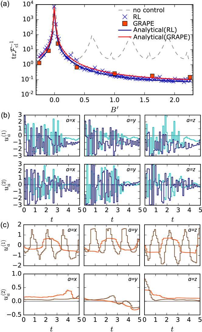
Figure 3: (a) Generalizability for the strength of the magnetic field in Example 1. For RL, we show $\operatorname{\tr\mathcal{F}_{\mathrm{cl}}^{-1}}$ at the target time $T=5$ as a function of $B^{\prime}$ in $[B-2\pi/T,B+2\pi/T]$ where $B=1$. We use the neural networks that are trained at $(B,\vartheta,\varphi)=(1,\pi/4,\pi/4)$ to generate the pulse sequences for $B^{\prime}$. The blue crosses show the results of RL. The red squares represent the results using new pulse sequences optimized by GRAPE. The solid dark blue (red) curve show the analytical results using the pulse sequences found by RL (GRAPE) at $(B,\vartheta,\varphi)=(1,\pi/4,\pi/4)$. The dashed gray curve shows the CR bound without control. (b) Representative pulse profiles obtained with RL. The cyan lines show the results of $B^{\prime}=B$. The purple lines show the results of $B^{\prime}=B+2\pi/T$. (c) Representative pulse profiles obtained with GRAPE. The red lines show the results of $B^{\prime}=B$. The brown lines show the results of $B^{\prime}=B+2\pi/T$.

Example 1. For the analytical method, due to Theorem 1, once we have the optimal control $\bm{u}^{(1)}$ for $\bm{B}$, we can update the control field as $\bm{u}^{(1)}\to\bm{u}^{(1)}-\quantity(\bm{B^{\prime}}-\bm{B})$ when the estimation of the parameter is updated to $\bm{B^{\prime}}$. At the same time, the RL policy is learned specifically at $\bm{B}$; then we generalize the trained policy network to the different magnetic field $\bm{B^{\prime}}$. In the simulation, the control fields and the RL agents are optimized at $(B,\vartheta,\varphi)=(1,\pi/4,\pi/4)$.

One of the simplest cases is that $\bm{B}$ and $\bm{B^{\prime}}$ are along the same direction. In Theorem 1 the matrix ${R}$ consists of the ratios ${R}_{BB}=1$, ${R}_{\vartheta\vartheta}=B^{\prime}/B$, and ${R}_{\varphi\varphi}=B^{\prime}/B$. All other elements are zero. The CR bound at the new value of the parameter is given by

$$\operatorname{\tr\mathcal{F}_{\mathrm{cl}}^{-1}}(\bm{B}^{\prime})=\delta\widehat{B}^{2}+\quantity(\frac{B}{B^{\prime}})^{2}\quantity(\delta\widehat{\vartheta}^{2}+\delta\widehat{\varphi}^{2}),$$ (20)

where $\delta\widehat{B}^{2}$, $\delta\widehat{\vartheta}^{2}$, and $\delta\widehat{\varphi}^{2}$ represent the diagonal terms of $\operatorname{\mathcal{F}_{\mathrm{cl}}^{-1}}(\bm{B})$. Here $\operatorname{\tr\mathcal{F}_{\mathrm{cl}}^{-1}}$ diverges at $B^{\prime}=0$, but with the increase of $B^{\prime}$ the value of $\operatorname{\tr\mathcal{F}_{\mathrm{cl}}^{-1}}$ decreases and it is lower bounded by $\delta\widehat{B}^{2}$.

Figure 3(a) shows the CR bound at the target time $T$ as a function of $B^{\prime}$, where $B^{\prime}$ is allowed to vary within $[B-2\pi/T,B+2\pi/T]$, while the direction of the magnetic field is fixed at $(\vartheta,\varphi)=(\pi/4,\pi/4)$. In Fig. 3(a) the dark blue and red solid lines correspond to the analytical scheme using the optimized controls obtained with RL and GRAPE, respectively, at $B=1$ (for the choice of the target time $T$ along with other details in the implementation of RL, see Appendix C). The results of evaluating the generalization of RL at different $B^{\prime}$ are shown by blue crosses. In addition, the CR bound obtained by rerunning the GRAPE procedure at selected $B^{\prime}$ is presented as red squares. The results of the CR bound from the generalization of RL are substantially lower than for the case without control in a large neighborhood around $B^{\prime}=1$, confirming the generalizability. In fact, for $B^{\prime}>1$, RL outperforms GRAPE, even if it is not trained or optimized specifically at those points. Moreover, the analytical scheme and the generalization of RL return similar values of the CR bounds, indicating that controls produced by a trained RL agent away from the training point is near optimal. For $|B^{\prime}|\lesssim 0.3$, no method offers notable improvement as the optimal solution diverges according to Eq. (20). We note that each of the GRAPE points costs on average more than or approximately $2$ h, meaning that rerunning the optimization in a range of $B^{\prime}$ would be prohibitively expensive. This demonstrates the effectiveness of RL and the analytical approaches.

Figure 3(b) shows representative pulse profiles found by RL, comparing the results found at the training point $B^{\prime}=B=1$ (cyan lines) and at a point away from the training point $B^{\prime}=B+2\pi/T$ (purple lines). Similarity between the two sets of pulses $\bm{u}^{(1)}$ is evident from the figure, suggesting that RL achieves generalizability through a mechanism similar to Theorem 1, i.e., the reversal of changes of the free evolution by adjusting available controls.

Fixing the strength $B$, we consider the change in the direction $(\vartheta,\varphi)$. Here we apply the change of variables transforming the spherical coordinates to Cartesian notation Yuan (2016). The Jacobian matrix and ${R}$ are much more complicated, and the classical Fisher information matrix is not necessarily diagonal for $\bm{B^{\prime}}$. Nevertheless, for $B^{\prime}=B=1$ and varying $(\vartheta^{\prime},\varphi^{\prime})$, the CR bound of $\bm{B^{\prime}}$ is given by

$$\operatorname{\tr\mathcal{F}_{\mathrm{cl}}^{-1}}(\bm{B}^{\prime})=C_{1}\delta\widehat{B}^{2}+C_{2}\delta\widehat{\vartheta}^{2}+C_{3}\delta\widehat{\varphi}^{2},$$ (21)

with

$$\begin{cases}C_{1}=\cos^{2}\vartheta+\sin^{2}\vartheta\quantity(\cos^{2}\Delta\varphi+\csc^{2}\vartheta^{\prime}\sin^{2}\Delta\varphi),\\ C_{2}=\sin^{2}\vartheta+\cos^{2}\vartheta\quantity(\cos^{2}\Delta\varphi+\csc^{2}\vartheta^{\prime}\sin^{2}\Delta\varphi),\\ C_{3}=\sin^{2}\vartheta\csc^{2}\vartheta^{\prime}\cos^{2}\Delta\varphi+\sin^{2}\vartheta\sin^{2}\Delta\varphi,\end{cases}$$

where $\Delta\varphi=\varphi^{\prime}-\varphi$ is the change in $\varphi$. This expression shows that $\Delta\varphi$ hardly shifts the optimal value of the CR bound, but $\vartheta^{\prime}$ has notable influences on the results. For example, if $\varphi^{\prime}=\varphi$ and $\vartheta^{\prime}$ varies, the CR bound would be

$$\operatorname{\tr\mathcal{F}_{\mathrm{cl}}^{-1}}(\bm{B}^{\prime})=\delta\widehat{B}^{2}+\delta\widehat{\vartheta}^{2}+{\color[rgb]{0,0,0}\sin^{2}{\vartheta}\csc^{2}{\vartheta^{\prime}}}\,\delta\widehat{\varphi}^{2},$$ (22)

and $\operatorname{\mathcal{F}_{\mathrm{cl}}^{-1}}(\bm{B}^{\prime})$ is block diagonal. The change of the parameter $\vartheta^{\prime}$ can have a strong influence on the estimation of $\varphi^{\prime}$. Specifically, the new lower bound $\delta\widehat{\varphi}^{\prime 2}$ has the smallest value at $\vartheta^{\prime}=\pi/2$ and diverges at $\vartheta^{\prime}=0,\pi$, i.e., the poles $\ket{0}$ and $\ket{1}$ on the Bloch sphere.

In Fig. 4 we show the results from the analytical scheme and the generalization of RL concerning the direction of the magnetic field, i.e., $\vartheta^{\prime}$ and $\varphi^{\prime}$ are varied within $[0,\pi]$ and $[0,2\pi]$, respectively. The strength of the magnetic field is fixed at $B=1$ and RL is trained at $(\vartheta,\varphi)=(\pi/4,\pi/4)$. Figure 4(a) shows the pseudo-color-plot of the CR bound. In a reasonably large neighborhood around the original training point $(\vartheta,\varphi)=(\pi/4,\pi/4)$, the RL-designed pulse sequences produce values of $\operatorname{\tr\mathcal{F}_{\mathrm{cl}}^{-1}}$ similar to those of the analytical method, indicating generalizability. Figure 4(b) and (c) each present a cut at fixed $\vartheta^{\prime}$ or $\varphi^{\prime}$ as indicated by the dashed lines in the right panel of Fig. 4(a). Figure 4(b) shows results with $\vartheta^{\prime}=\pi/4$ and $\varphi^{\prime}$ varying in $[0,2\pi]$. For the analytical method, it is clear that results initiated by RL have lower CR bounds as compared to the case with no control and GRAPE. This is also true in Fig. 4(c), which shows results with $\varphi^{\prime}=\pi/4$ and varying $\vartheta^{\prime}$ in $[0,\pi]$. Overall, quantum controls suppress the divergences that appear periodically in the no-control case at $\varphi^{\prime}=0,\pi$ or $\vartheta^{\prime}=\pi/2$, although the value of the CR bounds increases to infinity as $\vartheta^{\prime}$ approaches $0$ or $\pi$, as expected from Eq. (22). Scattered points showing results from GRAPE are found to be comparable to its corresponding analytical results, but we emphasize that here each point is a complete rerun of the full algorithm which is very expensive. On the other hand, RL provides suboptimal results with a much lower cost on the computational resources.

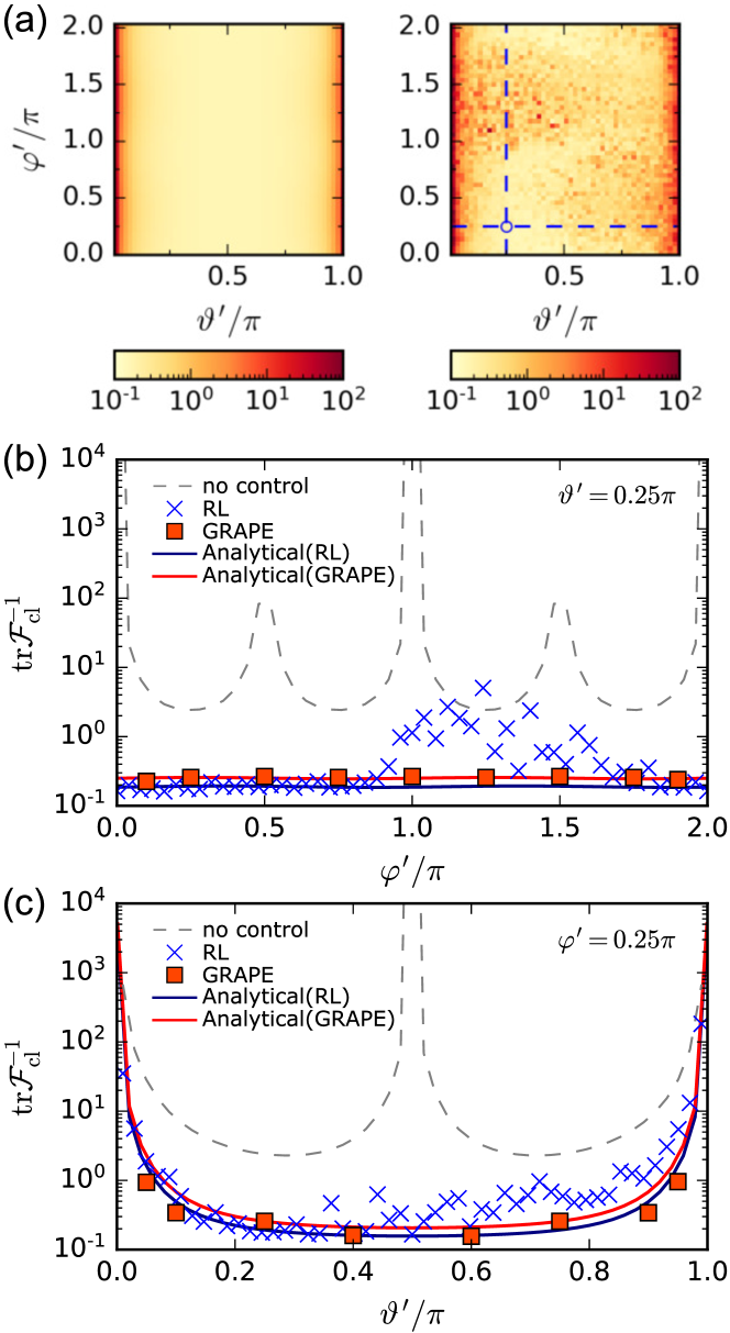
Figure 4: Generalizability for the direction of the magnetic field in Example 1. The strength of the magnetic field is fixed as $B=1$. (a) Pseudo-color-plots showing the CR bound $\operatorname{\tr\mathcal{F}_{\mathrm{cl}}^{-1}}$ at the target time $T=5$ as a function of the parameters $(\vartheta^{\prime},\varphi^{\prime})$ in the plane $[0,\pi]\times[0,2\pi]$. Note that the color bar has a logarithmic scale. Shown on the left is the CR bound using the analytical scheme. Shown on the right is the CR bound under controls generated by RL using the policy network trained at $(B,\vartheta,\varphi)=(1,\pi/4,\pi/4)$, the location of which is denoted by a blue circle. Two cuts (shown as blue dashed lines) correspond to the results in (b) and (c). (b) The CR bound as a function of $\varphi^{\prime}$ at fixed $\vartheta^{\prime}=0.25\pi$. (c) The CR bound as a function of $\vartheta^{\prime}$ at fixed $\varphi^{\prime}=0.25\pi$.

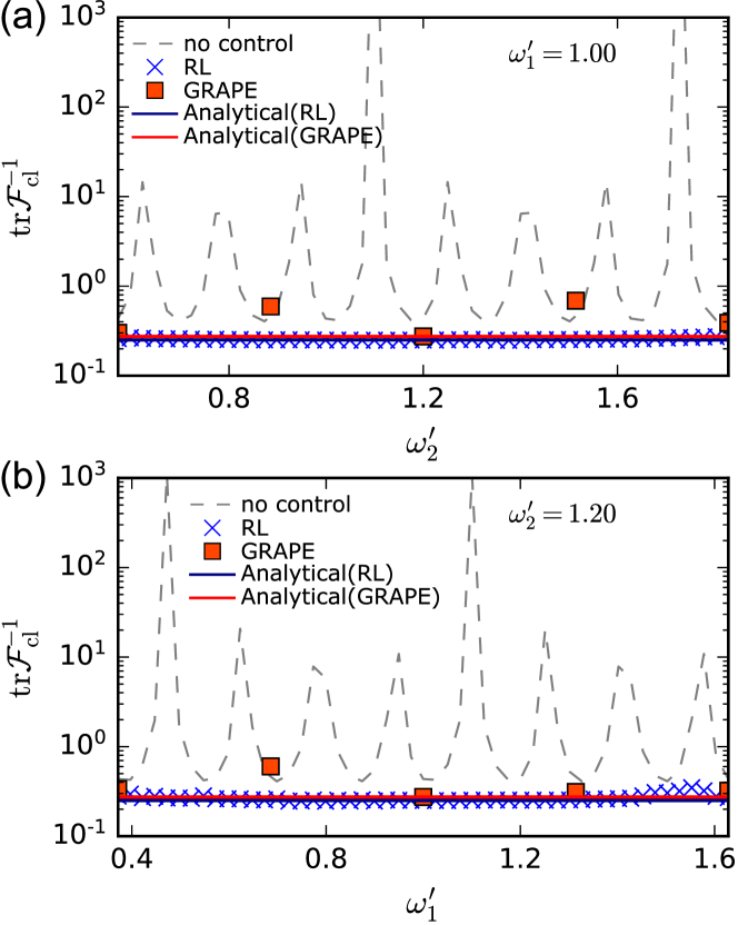
Figure 5: Generalizability for the individual magnetic fields in Example 2. The $ZZ$-coupling strength is fixed at $g=0.1$. (a) The CR bound as a function of $\omega_{2}^{\prime}$ at fixed $\omega_{1}^{\prime}=1.0$. (b) The CR bound as a function of $\omega_{1}^{\prime}$ at fixed $\omega_{2}^{\prime}=1.2$.

Example 2. The simplest case for coupling between qubits is the $ZZ$ coupling as in Eq. (10). Again, we introduce a change to the parameters $\bm{x}\to\bm{x}^{\prime}$, so $\delta H{(\bm{x},\bm{x^{\prime}})}=H_{0}(\bm{x}^{\prime})-H_{0}(\bm{x})=\sum_{k=1}^{2}\quantity(\omega_{k}^{\prime}-\omega_{k})\sigma_{z}^{(k)}+\quantity(g^{\prime}-g)\sigma_{z}^{(1)}\sigma_{z}^{(2)}$. When the individual magnetic fields $\omega_{k=1,2}$ change, it is straightforward to decompose the change $\delta H{(\omega_{k},\omega_{k}^{\prime})}$ into local controls $\sigma_{z}^{(k)}$. In the analytical scheme, control fields are adapted as $u_{z}^{(k)}\to u_{z}^{(k)}-\quantity(\omega_{k}^{\prime}-\omega_{k})$. Note that the partial derivative of $\omega_{k}\sigma_{z}^{(k)}$ with respect to $\omega_{k}$ is not a function of the parameter itself, i.e., ${R}=\mathbb{I}_{3}$ is a $3\times 3$ identity matrix. Thus, Theorem 1 proves that the optimal CR bound always stays at the same value $\operatorname{\tr\mathcal{F}_{\mathrm{cl}}^{-1}}(\bm{x}^{\prime})=\operatorname{\tr\mathcal{F}_{\mathrm{cl}}^{-1}}(\bm{x})$. For the generalization of RL, the RL agent is initially trained at the parameters $(\omega_{1},\omega_{2},g)=(1.0,1.2,0.1)$. Similar to Example 1, the trained RL agent will then be straightforwardly used on a range of $\omega_{1}^{\prime}$ and $\omega_{2}^{\prime}$.

In Fig. 5, we fix the $ZZ$-coupling strength and show the values of the CR bound with varying individual magnetic fields. To better illustrate the results, we fix one of $\omega_{1}^{\prime}$ and $\omega_{2}^{\prime}$ and vary the other. In Fig. 5(a), $\omega_{1}^{\prime}$ are fixed at 1.0 while $\omega_{2}^{\prime}$ varies, and in Fig. 5(b) we fix $\omega_{2}^{\prime}$ at 1.2 and change $\omega_{1}^{\prime}$. In both cases, the CR bounds obtained by the analytical method stay at constant values as noted above. Within the analytical scheme, initial controls obtained by RL give a slightly lower value of the CR bound. Meanwhile, RL shows a high level of generalizability since the CR bound is orders of magnitudes lower than that of no-control cases and is almost the same as those from the analytical method for a wide range of values. We have used GRAPE to optimize new control fields for selective $\omega_{k}^{\prime}$ and the results are represented by red squares. The fluctuation in the optimized values may arise from the fact that the optimization procedure of GRAPE might fall in a local minimum and that $f_{0}(T)$ [Eq. (12)] is different from the desired CR bound as noted in Sec. III.1.

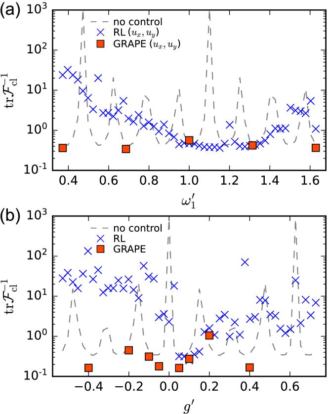
Figure 6: (a) Generalizability for the magnetic field using only the local controls $\sigma_{x}^{(1)}$, $\sigma_{y}^{(1)}$, $\sigma_{x}^{(2)}$ and $\sigma_{y}^{(2)}$. We show $\operatorname{\tr\mathcal{F}_{\mathrm{cl}}^{-1}}$ at the target time $T=5$ as a function of $\omega_{1}^{\prime}$ in $[1.0-\pi/T,1.0+\pi/T]$. The other parameters are fixed at $\omega_{2}^{\prime}=1.2$ and $g=0.1$. (b) Lack of generalizability for the $ZZ$-coupling strength. For RL, we show $\operatorname{\tr\mathcal{F}_{\mathrm{cl}}^{-1}}$ at the target time $T=5$ as a function of $g^{\prime}$ in $[0.1-\pi/T,0.1+\pi/T]$. The magnetic fields $\omega_{1}^{\prime}=1.0$ and $\omega_{2}^{\prime}=1.2$.

Under Example 2, we discuss two representative situations where the analytical method becomes inapplicable, where one must either apply GRAPE for each set of parameters or utilize the generalizability of RL.

In the first situation, we restrict the control channels to $\sigma_{x}^{(1)}$, $\sigma_{x}^{(2)}$, $\sigma_{y}^{(1)}$ and $\sigma_{y}^{(2)}$, so the shift $\delta H{(\omega_{k},\omega_{k}^{\prime})}\sim\sigma_{z}^{(k)}$ resulting from the change of $\omega_{k}$ can no longer be absorbed by local controls. In order to test the generalizability, the RL agent is trained at $(\omega_{1},\omega_{2},g)=(1.0,1.2,0.1)$ with the local controls $\sigma_{x}^{(1)}$, $\sigma_{y}^{(1)}$, $\sigma_{x}^{(2)}$, and $\sigma_{y}^{(2)}$. We study the magnetic field $\omega_{1}^{\prime}$ varying within $[1.0-\pi/T,1.0+\pi/T]$ while $\omega_{2}^{\prime}=1.2$. As shown in Fig. 6(a), the generalizability of RL is weaker, with reasonably low CR bounds seen in a smaller range $0.9\lesssim\omega_{1}^{\prime}\lesssim 1.3$ as a direct result of limited control channels.

In the second situation, the coupling strength $g$ changes and the analytical scheme no longer holds because the change $\delta H{(g,g^{\prime})}\sim\sigma_{z}^{(1)}\sigma_{z}^{(2)}$ cannot be simply decomposed into a combination of local controls, even with all control channels in Eq. (7) available. Figure 6(b) shows the CR bound under RL-designed controls as a function of $g^{\prime}$, which varies within $[0.1-\pi/T,0.1+\pi/T]$. The RL agent is trained at $(\omega_{1},\omega_{2},g)=(1.0,1.2,0.1)$. The values of the CR bound from RL are much higher than the no-control case, negating the generalizability with respect to the $ZZ$-coupling strength. Smaller values of the CR bound are attained by GRAPE, which means that the control fields now must be optimized for every individual $g^{\prime}$ using either GRAPE or RL but with the agent retrained at each individual new $g^{\prime}$ value. Practically, we note that quantum parameter estimation is not the only technique to measure the coupling strength. Taking the coupling between nuclear spins in molecules as an example, its magnitude can be determined by common splitting of spins and its sign can be found by spin-selective pluses Vandersypen and Chuang (2005). In other words, even if our generalizable quantum parameter estimation fails for the coupling between spins, our results on the strength of magnetic field $\omega_{k}$ are more relevant to experimental implementation.

V Conclusion

In this work we discussed the generalizability of the multiparameter quantum estimation schemes in two representative two-qubit systems in the presence of dephasing. Generalizability refers to a characteristic of a method that can derive from a known (initial) optimal control for a given set of parameters to the optimal control for another set of parameters, with minimal cost. The initial optimal control can be found by either RL or GRAPE. When the controls are complete, i.e., the shifts in the Hamiltonian due to change in parameters can be completely absorbed in the available control channels, one may generalize the optimal control using an analytical method. On the other hand, when the controls are limited such that these shifts cannot be completely absorbed in the available control channels, such as the case in which the control of a spin system is restricted to certain directions while the evolution of the spins does not have the restriction, the analytical scheme is invalid. However, RL retains a level of generalizability, albeit for a narrower range. Finally, if it is impossible to decompose the shift in the Hamiltonian into available controls, such as the $ZZ$ coupling of two spins in Example 2 considered here, neither RL nor the analytical scheme provides any generalizability and one must spend a great deal of resources to rerun either RL or GRAPE for each new set of parameters encountered. The analytical scheme provides important insight into when and how the generalizable optimal control of RL may be implemented, as the way RL generalizes controls is found to be similar to the analytical scheme. Our results should facilitate efficient implementation of optimal quantum estimation of multiple parameters, particularly for an ensemble of systems with ranges of parameters.

Appendix A Practical setup of RL

In the DDPG algorithm, the RL agent consists of a deep-$Q$ network denoted by $Q^{\mu}(s,a|\theta^{Q})$ and a (deterministic) policy network denoted by $\mu(s|\theta)$, which are parameterized by $\theta^{Q}$ and $\theta$ respectively. Here the state-action value function $Q^{\mu}\quantity(s_{j},a_{j})=\mathbb{E}\quantity[R_{j}|s_{j},a_{j}]$ describes the expected total discounted reward of state $s_{j}$ for taking the action $a_{j}$ Sutton and Barto (2018). The policy network has two hidden layers with 400 and 300 neurons, respectively. The deep-$Q$ network has two hidden layers with 400 and 300+$P$ neurons, respectively. Here $P$ represents the dimension of the action space, i.e., the number of control channels. Note that the second hidden layer in deep-$Q$ network concatenates the data from the output of its first hidden layer and the actions from the policy network. For both networks, the input layers take a 32-dimensional real vector corresponding to the fully known $4\times 4$ density matrix $\rho(j\Delta t)$. The elu activation function Paszke et al. (2019) is used after their hidden layers, and the final output layer of policy network uses tanh Paszke et al. (2019) to bound the actions.

The DDPG algorithm adapts two sets of neural networks similar to the deep-$Q$ learning: exploring the RL environment with one set of networks and training the other set (namely, the target networks) using the samples in a replay memory Mnih et al. (2013); Lillicrap et al. (2015). When performing the update to neural networks, we uniformly choose random samples from the replay memory so that the correlation between successive updates is removed, which reduces the variance of learning Sutton and Barto (2018). The Adam algorithm is used for the target deep-$Q$ and target policy networks with the learning rate $10^{-4}$ Paszke et al. (2019). Other hyperparameters are identical to the original DDPG paper Lillicrap et al. (2015).

In order to prevent the agent from learning undesirable solutions Sutton and Barto (2018), we define the reward function that has a nonzero value only at the target time $T$,

$$r_{j}=\begin{cases}0&{\color[rgb]{0,0,0}\text{for\quad}}j\neq N,\\ 100\sum_{n=1}^{4}10^{-10^{n}\operatorname{\tr\mathcal{F}_{\mathrm{cl}}^{-1}}}&{\color[rgb]{0,0,0}\text{for\quad}}j=N,\end{cases}$$ (23)

where the exponential encourages the agent to reduce $\operatorname{\tr\mathcal{F}_{\mathrm{cl}}^{-1}}$.

Appendix B Training procedure

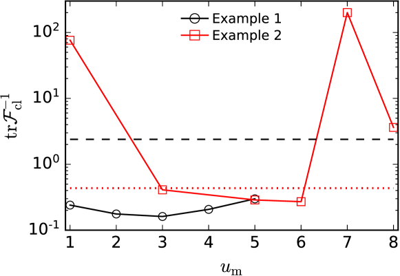
Figure 7: Performance of RL using different ranges of action space. We show the value of $\operatorname{\tr\mathcal{F}_{\mathrm{cl}}^{-1}}$ as a function of the range $u_{\mathrm{m}}$ where $|{u_{a}^{(i)}}|\leqslant u_{\mathrm{m}}$. The other parameters are $T=5$ and $\Delta t=0.1$. The same random seed is used. The black dashed and red dotted horizontals are the CR bound without control in Examples 1 and 2, respectively.

Training a neural network is usually time consuming, demanding heavy tuning of hyperparameters. In this section we investigate the performance of RL under different choices of the hyperparameters and exemplify the RL and GRAPE methods regarding their time complexity. The following simulations use the parameters $(B,\vartheta,\varphi)=(1,\pi/4,\pi/4)$ for Example 1 and $(\omega_{1},\omega_{2},g)=(1.0,1.2,0.1)$ for Example 2.

First, the controls in our simulation are piecewise square pulses where the strengths of controls, $u_{a}^{(i)}$, are directly relevant to the performance of RL. The range $|{u_{a}^{(i)}}|\leqslant u_{\mathrm{m}}$ significantly affects the efficiency and stability of the RL procedure. In Fig. 7 the results show that the range of control has little effect on $\operatorname{\tr\mathcal{F}_{\mathrm{cl}}^{-1}}$ at target time $T$ in Example 1, while the range can significantly affect the performance of RL in Example 2. From these results, we set the range as $|{u_{a}^{(i)}}|\leqslant 3$ in Example 1 and $|{u_{a}^{(i)}}|\leqslant 5$ in Example 2.

Second, we compare the training of RL using 2000, 10 000, and 20 000 RL episodes, with results shown in Fig. 8. For both Example 1 and Example 2 we have taken $T=5$ and $\Delta t=0.1$, so there are $50$ state-action pairs in each RL episode. The size of the replay memory is typically chosen as one-tenth of the total state-action pairs Mnih et al. (2013). The results show that in both cases, RL with fewer than 10 000 RL episodes fails to learn a good policy. In order to make the training satisfactory, we use 10 000 RL episodes with replay memory size of 50 000 in Example 1 and use 20 000 RL episodes with replay memory size 100 000 in Example 2. When $T$ is larger than $5$, longer RL training episodes and larger replay memory should be adapted accordingly.

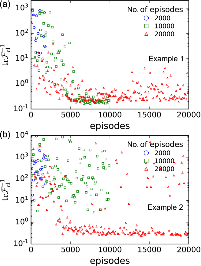
Figure 8: Training processes of RL in (a) Example 1 and (b) Example 2. Here $T=5$ and $\Delta t=0.1$. Blue marks represent results from a total of 2000 RL episodes with replay memory size 10 000, green marks correspond to a training involving 10 000 RL episodes with replay memory size 20 000, and red marks represent 20 000 RL episodes with replay memory size 100 000.

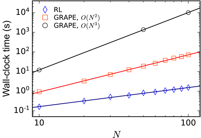
Figure 9: Time complexity of different methods. The $x$ axis shows the system size, i.e., the number of time slices $N$. The $y$ axis shows the wall-clock time cost in seconds. Diamonds on the blue line show the time cost in one RL training episode. Squares on the red line and circles on the black line are the times required by one iteration of GRAPE with and without storing the superoperators, respectively. Notice that the base-10 logarithmic scale is used for both axes.

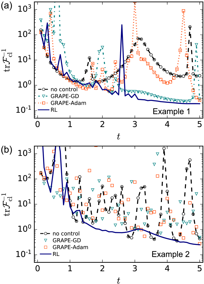
Figure 10: Classical CR bound $\operatorname{\tr\mathcal{F}_{\mathrm{cl}}^{-1}}$ as a function of $t$ in (a) Example 1 and (b) Example 2. The target time $T=5$. The parameters are $(B,\vartheta,\varphi)=(1,\pi/4,\pi/4)$ in Example 1 and $(\omega_{1},\omega_{2},g)=(1.0,1.2,0.1)$ in Example 2. The dashed black curves show the results without control. The solid blue curves show the results from RL. The dash-dotted green curves and the dotted orange curves represent results obtained by GRAPE with the steepest gradient ascent (GRAPE-GD) and Adam (GRAPE-Adam) methods, respectively. For GRAPE, the initial guess of the control is zero in Example 1 and the initial guess is random in Example 2.

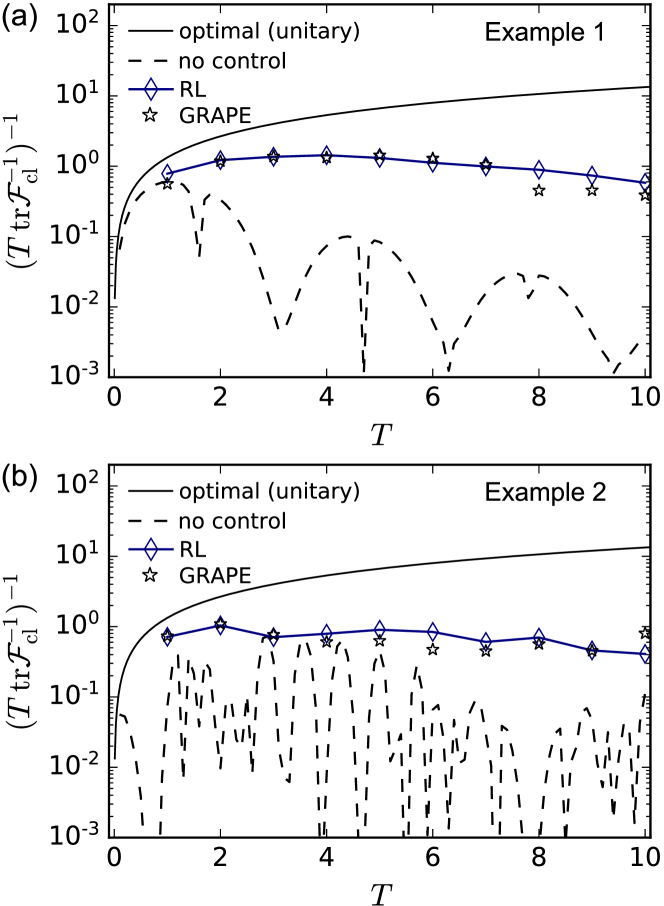
Figure 11: Plot of $\quantity(T\operatorname{\tr\mathcal{F}_{\mathrm{cl}}^{-1}})^{-1}$ as a function of the target time $T$ in (a) Example 1 with $(B,\vartheta,\varphi)=(1,\pi/4,\pi/4)$ and (b) Example 2 with $(\omega_{1},\omega_{2},g)=(1.0,1.2,0.1)$. Diamonds on the blue lines show results obtained by RL. Stars located at each $T$ are GRAPE results from Ref. Liu and Yuan (2017b). The dashed black curves show the value without control. The solid black curves represent the optimal precision limit $4T/3$ under unitary dynamics.

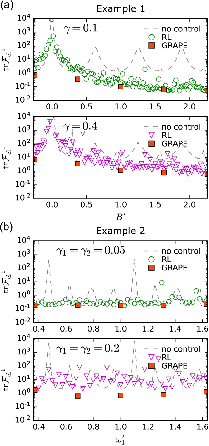
Figure 12: (a) Generalizability regarding the strength of the magnetic field in Example 1. Here $\operatorname{\tr\mathcal{F}_{\mathrm{cl}}^{-1}}$ evaluated at the target time $T=5$ is shown as a function of $B^{\prime}$ in $[B-2\pi/T,B+2\pi/T]$ where $B=1$. The RL agent is trained at $(B,\vartheta,\varphi)=(1,\pi/4,\pi/4)$ and the dephasing rate $\gamma=0.2$, which is subsequently used to generate control pulses for $B^{\prime}$ under dephasing rates $\gamma=0.1$ (upper panel) and $\gamma=0.4$ (lower panel). (b) Generalizability regarding individual magnetic fields in Example 2. The CR bounds evaluated at the target time $T=5$ are shown as a function of $\omega_{1}^{\prime}$ with fixed $\omega_{2}=1.2$ and coupling strength $g=0.1$. The RL agent is trained at $(\omega_{1},\omega_{2},g)=(1.0,1.2,0.1)$ and dephasing rates $\gamma_{1,2}=0.1$, which are subsequently used to generate control pulses for a range of $\omega_{1}^{\prime}$ under dephasing rates $\gamma_{1,2}=0.05$ (upper panel) and $\gamma_{1,2}=0.2$ (lower panel). The dashed gray curves show the CR bound without control for comparison.

Third, we discuss the time complexity of different methods as a function of $N$, the total number of time slices. As shown in Fig. 9, the RL method scales as $O{(N)}$. For the GRAPE methods, the slower one, $O{(N^{3})}$, has repeatedly calculated the master equation, but the faster one, $O{(N^{2})}$, uses more computer memory to store the superoperators. In general, RL requires about $10^{4}$ episodes to train an RL agent, but GRAPE needs about $10^{2}$ iterations to optimize a control field. For $T=5$ and $\Delta t=0.1$ used in this paper, $N=50$ and the total wall-clock time cost for RL and GRAPE to find the optimal control for a given set of parameters is actually comparable. We note that recent work suggests that the quantum version of the DDPG algorithm may offer a further speedup Wu et al. (2020).

Appendix C Implementation of RL

In this section we explain the details of the implementation of RL and compare the optimization from RL and GRAPE for both examples shown in Sec. II. While we largely follows Ref. Liu and Yuan (2017b) for GRAPE, we additionally apply the steepest gradient ascent method Ruder (2016) (results shown as GRAPE-GD) and the Adam method Kingma and Ba (2014) (results shown as GRAPE-Adam) to update the control field, which are numerically more efficient than the simple updating scheme. For RL, the state $s_{j}$ is a 32-dimensional vector corresponding to real and imaginary parts of elements in the $4\times 4$ density matrix $\rho(j\Delta t)$. The action $a_{j}$ is a six-dimensional vector consisting of elements in the control fields $\bm{u}^{(1)}(j\Delta t)$ and $\bm{u}^{(2)}(j\Delta t)$ on both qubits. For $j<N-1$, the immediate rewards are $r_{j+1}=0$, while $r_{N}$ is directly related to the CR bound $\operatorname{\tr\mathcal{F}_{\mathrm{cl}}^{-1}}$ (a detailed form is shown in Appendix A). In the RL procedure, the strength of the control field has a substantial impact on the outcome. A range is therefore imposed on the elements of control fields $u_{a}^{(i)}(t)\ (i=1,2)$ to avoid instability in the learning process. This range is set empirically as $|u_{a}^{(i)}|\leqslant 3$ for Example 1 and $|u_{a}^{(i)}|\leqslant 5$ for Example 2 as explained in Appendix B. No other restrictions on the RL procedure are imposed.

In Fig. 10(a) we show the values of the CR bound evolving from $t=0$ to the target time $t=T$ for Example 1 under quantum control. Overall, the CR bound is highest in the case of no control, indicating a low precision of the estimation. While all three methods produce lower CR bounds at the target time, spikes occur during the evolution using the GRAPE method, especially immediately before the target time. Instead, the precision under RL steadily saturates to the lowest value as the target time is reached. Results from RL is more desirable as in practice the time to implement the measurement may not be accurate Durkin (2010); Degen et al. (2017) and spikes in the CR bounds could result in a rather low precision when the measurement is not exerted precisely at the targeted time.

The time evolution of the CR bound for Example 2 is shown in Fig. 10(b). Again, results from RL steadily reach the lowest value, while results from all other methods are unstable over the course of the evolution. An interesting observation is that the result with no control is comparable to other methods at the target time, which may be due to the local measurement preventing all methods from reaching asymptotically optimal solutions Liu and Yuan (2017b); Liu et al. (2020); Humphreys et al. (2013); Szczykulska et al. (2016).

The CR bound under controls obtained from GRAPE fluctuates over the course of evolution because the control field is only optimized to minimize the bound at the final time. The RL agent, however, is trained to use samples from the replay memory, which breaks temporal correlation in each episode. In other words, the RL agent is trained to gradually steer states towards the final state. Therefore, as the system evolves close to the target time, the state is already very close to the final state, which is optimal for the estimation Liu and Yuan (2017a, b); Xu et al. (2019). This leads to less fluctuation in the results, as shown in Fig. 10. Therefore, although both RL and GRAPE are capable of finding optimal controls at the target time, results from RL have less fluctuation when the target time is approached, implying a certain level of robustness against the fluctuations in the time to exert the measurement.

Assuming that the target time is precisely known, we compare different methods on the optimized CR bound as a function of the final time $T$, namely, we allow $T$ to vary and use the reciprocal of the normalized CR bound, $\quantity(T\operatorname{\tr\mathcal{F}_{\mathrm{cl}}^{-1}})^{-1}$, for comparison. Under the unitary dynamics, the Heisenberg scaling can be attained for both examples Yuan (2016); Liu and Yuan (2017b), corresponding to $\quantity(T\operatorname{\tr\mathcal{F}_{\mathrm{cl}}^{-1}})^{-1}=4T/3$. In the presence of noises, $\quantity(T\operatorname{\tr\mathcal{F}_{\mathrm{cl}}^{-1}})^{-1}$ typically increases at the beginning of the evolution and decreases thereafter Liu and Yuan (2017b), suggesting that the averaged profit (each time unit) on the precision limit from the time evolution is maximal at a finite $T$, which is the optimal time to perform the measurement.

For Example 1, Fig. 11(a) shows the results of $\quantity(T\operatorname{\tr\mathcal{F}_{\mathrm{cl}}^{-1}})^{-1}$ vs $T$. As can be seen from the figure, the maximal value without control is achieved around $T\approx 1.2$, while the largest $\quantity(T\operatorname{\tr\mathcal{F}_{\mathrm{cl}}^{-1}})^{-1}$ obtained by RL occurs around $3\lesssim T\lesssim 5$, where the effect from control is maximized. As $T$ further increases, the accumulated dephasing effect becomes dominant and the controls may not optimally counteract the noise. For Example 2, Fig. 11(b) shows that without control, $\quantity(T\operatorname{\tr\mathcal{F}_{\mathrm{cl}}^{-1}})^{-1}$ attains the largest value around $T\approx 3$, but under RL the value of $\quantity(T\operatorname{\tr\mathcal{F}_{\mathrm{cl}}^{-1}})^{-1}$ fluctuates very little for $4\lesssim T\lesssim 6$, and tends to decrease for $T\gtrsim 6$. To ensure consistency, we have fixed $T=5$ for both examples in the main text. We also present GRAPE results using the same method of Ref. Liu and Yuan (2017b). As shown in Fig. 11, RL and GRAPE methods give comparable results for most values of $T$, with small differences at certain $T$ values.

Appendix D Generalizability under other values of the dephasing rates

In this appendix we study the generalizability of RL associated with varying values of the dephasing rates that are applied in both Example 1 and Example 2.

Figure 12(a) shows the CR bounds in Example 1 obtained as a function of varying magnetic field strength $B^{\prime}$ under different dephasing rates as indicated. The RL agent is trained at $(B,\vartheta,\varphi)=(1,\pi/4,\pi/4)$ and the dephasing rate $\gamma=0.2$, which is subsequently used to generate control pulses for $B^{\prime}$ under dephasing rates $\gamma=0.1$ (upper panel) and $\gamma=0.4$ (lower panel). For comparison, the CR bounds obtained by rerunning GRAPE at selected $B^{\prime}$ values are represented by squares, while the dashed curves show the CR bounds without control. As the dephasing rate becomes larger, the CR bound increases, indicating a lower precision due to enlarged noise as expected. For the smaller dephasing rate $\gamma=0.1$, the results from RL are comparable to those from GRAPE for $B^{\prime}>1$, even if the agent is not trained specifically at those values of $B^{\prime}$, indicating a good level of generalizability. For the larger dephasing rate $\gamma=0.4$, RL can no longer generate the pulse sequences as optimally as GRAPE, but the RL results are generally lower than the case without control for a wide range around $B^{\prime}=1$, suggesting that the generalizability is retained to a certain extent for larger dephasing rates. We emphasize that, for $|B^{\prime}|\sim 0$, no method provides a notable improvement as the optimal solution diverges according to Eq. (20).

Figure 12(b) shows the CR bounds in Example 2 obtained as a function of varying $\omega_{1}^{\prime}$ with $\omega_{2}^{\prime}$ fixed at 1.2 under different dephasing rates as indicated. The RL agent is trained at $(\omega_{1},\omega_{2},g)=(1.0,1.2,0.1)$ and the dephasing rate $\gamma_{1}=\gamma_{2}=0.1$, which is subsequently used to generate control pulses under dephasing rates $\gamma_{1}=\gamma_{2}=0.05$ (upper panel) and $\gamma_{1}=\gamma_{2}=0.2$ (lower panel). For the smaller dephasing rate $\gamma_{1,2}=0.05$, results from RL are similar to those from GRAPE, demonstrating a high level of generalizability as compared to the no-control case. On the other hand, for the larger dephasing rate $\gamma_{1,2}=0.2$, RL does not offer a notable improvement from the case without control and is inferior to GRAPE, implying that the generalizability is compromised by large noises. Enhancement of the ability of RL to accommodate large noises would be an important topic for further study, which would likely require more sophisticated techniques such as domain randomization Tobin et al. (2017) and network randomization Lee et al. (2020).

References

- Humphreys et al. (2013) P. C. Humphreys, M. Barbieri, A. Datta, and I. A. Walmsley, Phys. Rev. Lett. 111, 070403 (2013).
- Pezzè et al. (2017) L. Pezzè, M. A. Ciampini, N. Spagnolo, P. C. Humphreys, A. Datta, I. A. Walmsley, M. Barbieri, F. Sciarrino, and A. Smerzi, Phys. Rev. Lett. 119, 130504 (2017).
- Yue et al. (2014) J.-D. Yue, Y.-R. Zhang, and H. Fan, Sci. Rep. 4, 5933 (2014).
- Yuan and Fung (2017) H. Yuan and C.-H. F. Fung, npj Quantum Inf. 3, 14 (2017).
- Yuan and Fung (2015) H. Yuan and C.-H. F. Fung, Phys. Rev. Lett. 115, 110401 (2015).
- Liu and Yuan (2017a) J. Liu and H. Yuan, Phys. Rev. A 96, 012117 (2017a).
- Pang and Jordan (2017) S. Pang and A. Jordan, Nat. Commun. 8, 14695 (2017).
- Fraïsse and Braun (2017) J. M. E. Fraïsse and D. Braun, Phys. Rev. A 95, 062342 (2017).
- Fiderer et al. (2019) L. J. Fiderer, J. M. E. Fraïsse, and D. Braun, Phys. Rev. Lett. 123, 250502 (2019).
- Haine and Hope (2020) S. A. Haine and J. J. Hope, Phys. Rev. Lett. 124, 060402 (2020).
- Yuan (2016) H. Yuan, Phys. Rev. Lett. 117, 160801 (2016).
- Liu and Yuan (2017b) J. Liu and H. Yuan, Phys. Rev. A 96, 042114 (2017b).
- Khaneja et al. (2005) N. Khaneja, T. Reiss, C. Kehlet, T. Schulte-Herbrüggen, and S. J. Glaser, J. Magn. Reson. 172, 296 (2005).
- Mnih et al. (2013) V. Mnih, K. Kavukcuoglu, D. Silver, A. Graves, I. Antonoglou, D. Wierstra, and M. Riedmiller, arXiv:1312.5602.
- Mnih et al. (2015) V. Mnih, K. Kavukcuoglu, D. Silver, A. A. Rusu, J. Veness, M. G. Bellemare, A. Graves, M. Riedmiller, A. K. Fidjeland, G. Ostrovski, et al., Nature (London) 518, 529 (2015).
- Silver et al. (2016) D. Silver, A. Huang, C. J. Maddison, A. Guez, L. Sifre, G. van den Driessche, J. Schrittwieser, I. Antonoglou, V. Panneershelvam, M. Lanctot, S. Dieleman, D. Grewe, J. Nham, N. Kalchbrenner, I. Sutskever, T. Lillicrap, M. Leach, K. Kavukcuoglu, T. Graepel, and D. Hassabis, Nature (London) 529, 484 (2016).
- Fösel et al. (2018) T. Fösel, P. Tighineanu, T. Weiss, and F. Marquardt, Phys. Rev. X 8, 031084 (2018).
- Bukov et al. (2018) M. Bukov, A. G. R. Day, D. Sels, P. Weinberg, A. Polkovnikov, and P. Mehta, Phys. Rev. X 8, 031086 (2018).
- Niu et al. (2019) M. Y. Niu, S. Boixo, V. N. Smelyanskiy, and H. Neven, npj Quantum Inf. 5, 33 (2019).
- Zhang et al. (2019) X.-M. Zhang, Z. Wei, R. Asad, X.-C. Yang, and X. Wang, npj Quantum Inf. 5, 85 (2019).
- Lin et al. (2020) J. Lin, Z. Y. Lai, and X. Li, Phys. Rev. A 101, 052327 (2020).
- Xu et al. (2019) H. Xu, J. Li, L. Liu, Y. Wang, H. Yuan, and X. Wang, npj Quantum Inf. 5, 82 (2019).
- Schuff et al. (2020) J. Schuff, L. J. Fiderer, and D. Braun, New J. Phys. 22, 035001 (2020).
- Fiderer et al. (2021) L. J. Fiderer, J. Schuff, and D. Braun, PRX Quantum 2, 020303 (2021).
- Sutton and Barto (2018) R. S. Sutton and A. G. Barto, Reinforcement Learning: An Introduction (MIT Press, Cambridge, 2018).
- Tobin et al. (2017) J. Tobin, R. Fong, A. Ray, J. Schneider, W. Zaremba, and P. Abbeel, in Proceedings of the 2017 IEEE/RSJ International Conference on Intelligent Robots and Systems (IROS), Vancouver, 2017 (IEEE, Piscataway, 2017) pp. 23–30.
- Lee et al. (2020) K. Lee, K. Lee, J. Shin, and H. Lee, in International Conference on Learning Representations (ICLR) (2020).
- (28) Sutton, Richard S, Generalization in reinforcement learning: Successful examples using sparse coarse coding in Advances in Neural Information Processing Systems 8, edited by D. S. Touretzky and M. C. Mozer and M. E. Hasselmo (MIT Press, Cambridge, 1996) pp. 1038–1044.
- Cobbe et al. (2019) K. Cobbe, O. Klimov, C. Hesse, T. Kim, and J. Schulman, in Proceedings of the 36th International Conference on Machine Learning, Proceedings of Machine Learning Research, Vol. 97, edited by K. Chaudhuri and R. Salakhutdinov (PMLR, 2019) pp. 1282–1289.
- Zhang et al. (2018) A. Zhang, N. Ballas, and J. Pineau, arXiv:1806.07937.
- Packer et al. (2019) C. Packer, K. Gao, J. Kos, P. Krähenbühl, V. Koltun, and D. Song, arXiv:1810.12282.
- Pathak et al. (2017) D. Pathak, P. Agrawal, A. A. Efros, and T. Darrell, in Proceedings of the IEEE Conference on Computer Vision and Pattern Recognition Workshops, Honolulu, 2017 (IEEE, Piscataway, 2017), pp. 16–17.
- Breuer and Petruccione (2002) H.-P. Breuer and F. Petruccione, The Theory of Open Quantum Systems (Oxford University Press, Oxford, 2002).
- Liu et al. (2020) J. Liu, H. Yuan, X.-M. Lu, and X. Wang, J. Phys. A: Math. Theor. 53, 023001 (2020).
- Ruder (2016) S. Ruder, arXiv:1609.04747.
- Kingma and Ba (2014) D. P. Kingma and J. Ba, arXiv:1412.6980.
- (37) D. Silver, G. Lever, N. Heess, T. Degris, D. Wierstra, and M. Riedmiller, in Proceedings of the 31st International Conference on Machine Learning, Beijing, 2014, edited by Eric P. Xing and Tony Jebara (Microtome, Brookline, 2014) pp. 387–395.
- Lin (1993) L.-J. Lin, Reinforcement learning for robots using neural networks, Tech. Rep. (Carnegie-Mellon Univ Pittsburgh PA School of Computer Science, 1993).
- Lillicrap et al. (2015) T. P. Lillicrap, J. J. Hunt, A. Pritzel, N. Heess, T. Erez, Y. Tassa, D. Silver, and D. Wierstra, arXiv:1509.02971.
- Leonhardt (1997) U. Leonhardt, Measuring the Quantum State of Light, (Cambridge University Press, Cambridge, 1997), Vol. 22.
- James et al. (2001) D. F. V. James, P. G. Kwiat, W. J. Munro, and A. G. White, Phys. Rev. A 64, 052312 (2001).
- Vandersypen and Chuang (2005) L. M. K. Vandersypen and I. L. Chuang, Rev. Mod. Phys. 76, 1037 (2005).
- Paszke et al. (2019) A. Paszke, S. Gross, F. Massa, A. Lerer, J. Bradbury, G. Chanan, T. Killeen, Z. Lin, N. Gimelshein, L. Antiga et al., in Advances in Neural Information Processing Systems 32: Proceedings of the 33rd Conference on Neural Information Processing Systems, Vancouver, 2019, edited by H. Wallach, H. Larochelle, A. Beygelzimer, F. d’ Alché-Buc, E. Fox, and R. Garnett (Curran, Red Hook, 2019) pp. 8024–8035.
- Wu et al. (2020) S. Wu, S. Jin, D. Wen, and X. Wang, arXiv:2012.10711.
- Durkin (2010) G. A. Durkin, New J. Phys. 12, 023010 (2010).
- Degen et al. (2017) C. L. Degen, F. Reinhard, and P. Cappellaro, Rev. Mod. Phys. 89, 035002 (2017).
- Szczykulska et al. (2016) M. Szczykulska, T. Baumgratz, and A. Datta, Adv. Phys. X 1, 621 (2016).