Epidemic spreading

Abstract

We present an analysis of six deterministic models for epidemic spreading. The evolution of the number of individuals of each class is given by ordinary differential equations of the first order in time, which are set up by using the laws of mass action providing the rates of the several processes that define each model. The epidemic spreading is characterized by the frequency of new cases, which is the number of individuals that are becoming infected per unit time. It is also characterized by the basic reproduction number, which we show to be related to the largest eigenvalue of the stability matrix associated with the disease-free solution of the evolution equations. We also emphasize the analogy between the outbreak of an epidemic with a critical phase transition. When the density of the population reaches a critical value the spreading sets in, a result that was advanced by Kermack and McKendrick in their study of a model in which the recovered individuals acquire permanent immunization, which is one of the models analyzed here.

I Introduction

The control and possibly the eradication of an infectious disease is not fully successful without the knowledge of the mechanisms that determine its spreading in a population. A major contribution in this direction is provided by the theoretical study of epidemic spreading through the use of deterministic and stochastic models. The theoretical study of the epidemic spreading bailey1957 ; anderson1991 ; renshaw1991 ; mollison1995 ; hastings1997 ; keeling2008 is not new but it did not properly start before the physical basis for the causes of the infectious disease was established in the second half of the nineteenth century bailey1957 . By the end of the nineteenth century the mechanism of epidemic spreading, revealed by bacteriology, allowed the development of the first epidemic models bailey1957 .

Hammer in 1906, carried out an analysis of the measles epidemic considering that the infection spreads from person to person and depends on the number of the susceptible bailey1957 . In his studies of the relation between the number of mosquitoes and the incidence of malaria, Ross starting from 1908 formulated models for the transmission of the infectious diseases bailey1957 . In his book on the prevention of malaria of 1911 ross1911 , he employed ordinary differential equations to describe the evolution of the number of affected and unaffected individuals by a disease, and wrote the equations in terms of rates of several types, pointing out the major role of the infection rate.

A more general theory than that of Ross, but employing similar ideas, was developed by Kermack and McKendrick in 1927 kermack1927 . They proposed a model for an epidemic consisting of recovered individuals having permanent immunization. They were able to solve the differential equations that governs the time evolution of the number of susceptible, infected, and recovered, arriving at a remarkable theorem concerning the spreading threshold of an epidemic bailey1957 ; kermack1927 . If the density of the susceptible is smaller than a certain value, the epidemic does not outbreak. In other terms, if the infection rate is smaller than a critical value the disease does not spread.

In 1929, Soper developed deterministic models for measles by using difference equations bailey1957 , and by assuming that the operations of transmission are analogous to the mass law action of chemistry soper1929 . The equations developed by Kermack and McKendrick were also in accordance with this law which would become one of the most important concepts in theoretical epidemiology anderson1991 .

The deterministic models, employing ordinary differential equations, were carried further mainly after around 1945 bailey1957 . In 1952, Macdonald introduced a concept, which he called basic reproduction rate, concerning the threshold of spreading, with reference to the threshold theorem of Kermack and McKendrick macdonald1952 ; heesterbeek2015 . However, it was not before 1975 when the concept was reintroduced by Hethcote and by Dietz, that it became widely used heesterbeek2002 .

Around 1945, the stochastic approach for epidemic spreading, which had been originated earlier, received further development by Bartlett bailey1957 . He transformed the Kermack and McKendrick epidemic model into a stochastic model by treating the numbers of susceptible and infective individuals as stochastic variables bartlett1949 . The corresponding master equation in these two variables was obtained by Bailey bailey1957 ; bailey1953 and the stochastic version of the Kermack and McKendrick threshold theorem was advanced by Whittle whittle1955 . The model included two processes: the recovery of infected individual, who acquires permanent immunization, and the infection of a susceptible by the contact with an infective individual. These stochastic models can be understood as discrete generic random walk in a space whose axes are the numbers of various classes of individuals nisbet1982 ; tome2015L .

A distinct type of stochastic models for epidemic spreading takes into account the spatial structure in which real infectious diseases spread in a population harris1974 ; grassberger1983 ; grassberger1983a ; ohtsuki1986 ; satulovsky1994 ; durrett1995 ; antal2001 ; dammer2003 ; souza2010 ; tome2011 ; souza2013 ; tome2015 ; ruziska2017 . The spatial stochastic models are formulated in terms of several stochastic variables, one for each individual, and which take values corresponding to the class an individual belongs in with respect to the disease tome2015L . Usually, they are defined on a lattice that represents the spatial structure.

The spatial stochastic model allows us to derive the stochastic model of the generic random walk mentioned above by a suitable reduction of stochastic variables. This reduction can be made at the first level, represented by the numbers of individuals of each class, or at the second level, which takes into account the pairs of individuals tome2009 ; tome2011 . It is also possible from the spatial stochastic models to reach the deterministic evolution equations at the first level, which are the usual evolution equations such as the ones studied here, or at the second level where the numbers of pairs of individuals are taken into account satulovsky1994 ; souza2013 ; ana2017 .

Here we only consider the deterministic approach to the epidemic spreading, which still is a relevant approach to the study of epidemic spreading of various infectious diseases adriana2006 ; burattini2008 ; pinho2010 . We analyze models that are appropriate for the direct transmission of the disease, that is, when the transmission occurs from person to person, which is the case of most common infectious diseases such as measles, chickenpox, mumps, rubella, smallpox, common cold, and influenza, as well as the present covid-19. These models include the susceptible-infected-susceptible (SIS) ross1911 , the susceptible-infected-recovered (SIR) kermack1927 , and the susceptible-exposed-infected-recovered (SEIR) dietz1976 . The models that we considered here are those such that the total number of individuals is constant in time. We do not consider demographic processes, such as birth, death, and migration.

We present the main features that are used to characterize the spreading such as the reproduction number and the frequency of new cases, which is called the epidemic curve when it is plotted as a function of time. Our presentation emphasizes the analogy with the thermodynamic phase transition, the onset of spreading being understood as the critical point of a continuous thermodynamic phase transition, when the epidemic comes to an end, in which case the frequency of new cases vanishes, the size of the epidemic can be measured by the area under the epidemic curve, and can be understood the order parameter.

The spatial stochastic version of the SIS model was proposed by Harris harris1974 , who named it the contact process. It is widely studied not only because it describes an epidemic spreading but also because of its critical behavior grassberger1983a which is distinct from models describing system in thermodynamic equilibrium such as the Ising model tome2015L ; marro1999 ; henkel2008 . The SIS model describes the evolution of an infectious disease that becomes endemic. The simplest model that describes the evolution of a infectious disease that becomes extinct is the SIR model. Its spatial version was formulated by Grassberger grassberger1983 , who called it general epidemic process, and its critical behavior is distinct from the Ising model and also different from the SIS model tome2015L ; marro1999 ; henkel2008 .

It is worth pointing out that the approach to epidemic spreading, be it deterministic or stochastic, is extended to a more general context of the population dynamics tome2015L ; ribeiro2017 ; cunha2017 , as for instance in ecological problems such as the predator-prey dynamics satulovsky1994 ; tome2015L .

II Evolution equations

The spreading of an epidemic is understood as the time evolution of a population consisting of several classes of individuals pertaining to a certain community. The two main classes of individuals are the susceptible and the infective but other classes may also be present. As the epidemic evolves in time, an individual belonging in one class might change to another class through a transforming process. We remark that the members of the infective class are individuals that infect others. An individual that is infected by a disease but does not infect others belong in a distinct class, the exposed class.

The framework that is used here to analyze the population dynamics is borrowed from the theory of chemical kinetics. According to this theory, molecules of various species inside a vessel are subject to chemical reactions that transform molecules of one species into molecules of another species. The several classes of individuals are analogous to the chemical species, and the processes that transform an individual of one class to an individual of another class are analogous to chemical reactions.

As an example of the analogy, let us consider the process where an infective (I) individual recovers from the disease becoming a recovered (R) individual. This process is represented by

$${\rm I}\longrightarrow{\rm R},$$ (1)

which is understood as a reaction that transforms one I into one R, or the annihilation of one I and the simultaneous creation of one R. This type of reaction is called spontaneous.

Another example is the process of infection of a susceptible (S) individual who become infected by the contact with an infective (I) individual It is represented by

$${\rm S}\stackrel{{\scriptstyle\rm I}}{{\longrightarrow}}{\rm I},$$ (2)

where the symbol I over the arrow means that the reaction that transforms one S into one I needs the presence of one I. This type of reaction is called catalytic or more precisely auto-catalytic and I is the catalyst.

After introducing the analogy between chemical species and chemical reactions, on one side, and classes of individuals and transforming process, in the other, we introduce a second analogy. The time evolution of the numbers of individuals of each class, determined by the transforming processes, are understood as analogous to the chemical kinetic equations. These are ordinary differential equations of the first order in time involving the concentrations or the fractions of the various chemical species and are set up by the use of the law of mass action.

The primary question one wants to answer is how many individuals are there in each class. Thus we should seek for equations in the number of individuals in each class. However, it is more convenient to express the equations in terms of the density, which is the number of individuals per unit area, or in terms of the fraction of individuals in each class. To set up the evolution equations in either one of these two types of variables, we will employ the law of mass action, presented and explained in the Appendix. Here, we choose to write down the equations in terms of the fractions of each class of individuals.

As an example of the application of the law of mass action, consider the infection process represented by equation (2), and let us denote by $x$ the fraction of the susceptible and by $y$ the fraction of the infective. The contribution of this process to the evolution equation of both $x$ and $y$, in accordance with the law of mass action, is $bxy$, where $b$ is the infection rate constant, that is,

$$\frac{dx}{dt}=-bxy+\ldots,$$ (3)

$$\frac{dy}{dt}=bxy+\ldots,$$ (4)

where the dots indicate the contribution coming from other processes. Notice the presence of a minus sign in the first equation, because the number of the susceptible decreases in the infection process.

The evolution equations describing an epidemic consist of two or more equations that give the time variation of the fractions of the several classes of individuals. We assume that the total number of individuals is constant, so that the sum of all fractions equals one. They are solved with an initial condition that reflects what occurs in a real epidemic. At the beginning, all individuals are susceptible except a very small fraction of them that are infective.

Our presentation uses frequently the term rate, as in infection rate. It should not be confused with the variation in time, which is a derivative. One should also make a distinction between a rate and a rate constant which appears as a prefactor of a rate.

III Characterization

III.1 Epidemic curve

A relevant characterization of the evolution of an epidemic is the frequency of the number of individuals that are becoming infected, or the number of newly infected individuals per unit time, or simply the frequency of new cases. The ratio of this number and the total number of individuals we denote by $f$. When $f$ is plotted as a function of the time it is called the epidemic curve. The curve initially grows exponentially until an inflexion point after which it behaves in such a way as to reach a final value which may be zero, in which case the epidemic comes to an end, or nonzero, in which case the disease becomes endemic.

To determine $f$, we consider all processes of the type

$${\rm A}\stackrel{{\scriptstyle\rm I}}{{\longrightarrow}}{\rm B},$$ (5)

where B represents an infected and A a non-infected individual. We then use the law of mass action to determined the rate of this process. The sum of the rates of all process of this type is $f$. In the case of the auto-catalytic process of the preceding section, in which an S is transformed into one I, the frequency of new cases is $f=bxy$.

III.2 Phase transition

The spreading of a disease can be viewed as a thermodynamic phase transition. To understand this point we consider that the infection rate constant, denoted by $b$, takes several values. For small values, there is no spreading whereas for large values the epidemic spreads. Increasing $b$, one passes from a non-spreading regime to a spreading regime at a critical value $b_{c}$ that gives the onset of spreading. This condition may seem to make no reference to the closeness of the individuals, or equivalently to the density of the population. In a real process of infection, the contact, or at least the proximity of two individuals, is an important condition for the onset of spreading. Thus this feature should in some way be included in the theory. In fact, this is the case, as explained next.

In the Appendix, it is shown that the infection rate constant $b$ is proportional to the intrinsic rate constant $b^{*}$, that is,

$$b=\gamma b^{*},$$ (6)

where $\gamma$ is the ratio of the total number of individuals in a community and the area of the community, or the population density. The intrinsic rate constant $b^{*}$ is a measure of the strength of infection or the virulence of the disease and is density-independent. Let us define the critical density $\gamma_{c}=b_{c}/b^{*}$ and see what happens when one increases $\gamma=b/b^{*}$. When $\gamma$ increases, $b$ increases, and when it reaches the value $\gamma_{c}$, the rate constant reaches the critical value $b_{c}$, and the spreading outbreaks. In other words, when the density of the population reaches a critical value, the disease outbreaks. This is, in fact, the statement of the Kermack and McKendrick theorem, except that they refer to the density of the susceptible but at the beginning of spreading the population consist mostly of the susceptible.

It is usual to characterize the transition from a trivial phase to the significant phase by an order parameter, which is nonzero for the significant phase and zero for the trivial one. For the cases of an epidemic spreading that comes to an end, so that the frequency of new cases $f$ vanishes for the long term, the order parameter may be defined as the area $s$ of the epidemic curve,

$$s=\int_{0}^{\infty}fdt,$$ (7)

where $f$ here is understood as function of $t$.

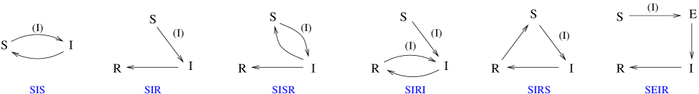
Figure 1: Representation of the processes involved in each epidemic spreading model. The classes of individuals are: susceptible (S), infective (I), recovered (R), and exposed (E). An I between parentheses indicates that the process is catalytic and I is the catalyst. The other processes are spontaneous. An exposed individual is infected but not infective. A recovered individual has permanent immunity in the SIR, SISR, and SEIR models.

III.3 Reproduction number

Another important characterization of the epidemic spreading is related to the number of individuals that are infected by a single infective individual. This number, called the reproduction number and denoted by $R$, is the ratio of two numbers and is defined more precisely as follows. During an interval of time $\tau$, the number of new cases is $N_{1}=fN\tau$, where $f$ is the frequency of new cases defined above and $N$ is the total number of individuals.

The question now arises about the number $N_{2}$ of the infective that are responsible for these new infections. If the number of the infective remains the same in the interval $\tau$, then $N_{2}$ would be equal to $N_{1}$. But if the infective increases by a certain amount $N_{3}$ then $N_{2}$ should be smaller, and in fact equal to $N_{1}-N_{3}$, and $R=N_{1}/(N_{1}-N_{3})$. In view that $N_{3}=N(dy/dt)\tau$, where $y$ is the fraction of infective we find

$$R=\frac{f}{f-dy/dt}.$$ (8)

As $f$ is the rate of a catalytic process, in which the infective is the catalyst, $f$ is proportional to $y$, that is, $f=gy$, which allows us to write

$$R=\frac{g}{g-d\ln y/dt}.$$ (9)

The basic reproduction number, denoted by $R_{0}$, is the reproduction number at the early stages of the spreading when the number of infective individuals is negligible and the whole population consists mostly of susceptible. Thus $R_{0}$ is obtained from $R$ by setting $x=1$ in the formula (9).

It is worth mentioning at this point a fundamental property that should be obeyed by the equations describing an epidemic. As the spreading of the disease needs the presence of an infected, then if $y=0$ there is no evolution meaning that the other variables should not vary in time. Therefore, the state consisting of $y=0$ and other variables constant should be a solution of the evolution equation. This state is the trivial solution and is called disease-free solution. In stochastic models, it is called absorbing state.

The stability analysis of the trivial solution is a way of determining the outbreak of the spreading. Linear stability reveals that the fraction of infective $y$ is dominated by the exponential behavior, $y=y_{0}e^{\alpha t}$, where $\alpha$ is the largest eigenvalue of the stability matrix. The onset of spreading occurs when $\alpha$ turns from a negative to a positive value. Thus, at the early stages of the spreading $y=y_{0}e^{\alpha t}$ and $x$ near one. Replacing these results in equation (9) we reach a relationship between the basic reproduction number and the exponent $\alpha$, which is

$$R_{0}=\frac{g_{0}}{g_{0}-\alpha},$$ (10)

where $g_{0}$ is the value of $g$ when $x=1$. As the onset of spreading occurs when $\alpha=0$, we see that the outbreak of spreading occurs at $R_{0}=1$, When $\alpha>0$, that is, when $R_{0}>1$, the epidemic spreads.

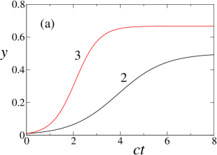
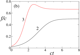
Figure 2: SIS model. (a) Fraction $y$ of infective individuals as a function of time $t$, for the values of $b/c$ indicated. (b) Epidemic curve, which is the frequency $f$ of new cases as a function of time $t$, for the values of $b/c$ indicated. (c) Order parameter $s$ versus the infection rate constant $b$. The order parameter is the fraction of individuals that remain infected for long times.

IV Models of spreading

The models that we will analyze consist of two or three processes involving two or more classes of individuals. They are represented by a flow diagram which gives all the possibilities of transformation of the individual from one class to another. The six models that we analyze are shown in figure 1.

IV.1 SIS model

We start by considering the simplest model for epidemic spreading which consists of two classes of individuals: infective (I) and susceptible (S). The model comprises two transformation processes. In the first, a susceptible individual becomes infective by the contact with other infective individuals. This process is represented by

$${\rm S}\stackrel{{\scriptstyle\rm I}}{{\longrightarrow}}{\rm I},$$ (11)

and occurs with an infection rate constant $b$. In the second, an infective individual becomes susceptible spontaneously. More specifically, an infective individual that has recovered from the disease does not acquire immunity becoming immediately susceptible again. This process is represented by

$${\rm I}\longrightarrow{\rm S},$$ (12)

occurring with a recovery rate constant $c$.

We denote by $x$ and $y$ the fraction of the susceptible and infective, respectively. As only these two classes of individuals are present, the sum of these two fractions equals one, $x+y=1$. According to the rules of mass action, the equation that gives the evolution of $x$ and $y$ are

$$\frac{dx}{dt}=-bxy+cy,$$ (13)

$$\frac{dy}{dt}=bxy-cy.$$ (14)

Due to the constraint $x+y=1$, these equations are not independent. Replacing $x$ by $1-y$ in equation (14), it becomes

$$\frac{dy}{dt}=\alpha y-by^{2},$$ (15)

where $\alpha=b-c$.

One solution of this equation is the trivial solution $y=0$, and therefore $x=1$, which is understood as the absence of epidemic spreading because there are no infective individuals present. To find whether this solution is stable one tries to solve the equation (15) for small values of $y$. The term proportional do $y^{2}$ is neglected and the equation becomes the linear equation

$$\frac{dy}{dt}=\alpha y,$$ (16)

whose solution is

$$y=y_{0}e^{\alpha t},$$ (17)

where $y_{0}$ is the value of $y$ at $t=0$. Therefore, if $\alpha>0$, that is, if $b>c$, then the number of infective increases exponentially and the spreading of the disease sets in. If $\alpha<0$, the disease does not spread. Recalling that $\alpha=b-c$, it follows that $b=c$ marks the onset of spreading. If $b>c$ the epidemic spreads and if $b<c$ it does not.

The equation (15) can in fact be solved in a closed form by writing it in the differential form as

$$dt=\frac{dy}{y(\alpha-by)},$$ (18)

or yet as

$$\alpha dt=\frac{dy}{y}+\frac{bdy}{\alpha-by}.$$ (19)

Integrating we find

$$\alpha t=\ln y-\ln(\alpha-by)+k,$$ (20)

where we are considering solutions such that $\alpha\geq by$. Let us suppose that at $t=0$, the number of infective is $y_{0}$. This determines the constant $k$ and we may write

$$y=\frac{\alpha y_{0}}{by_{0}+(\alpha-by_{0})e^{-\alpha t}},$$ (21)

which gives $y$ as a function of $t$.

We distinguish two types of solutions depending on the sign of $\alpha$. Let us consider that $\alpha<0$. As we have seen above, in this case there is no spreading of the disease. The right-hand side of equation (15) is negative and $y$ will decrease toward its asymptotic value $y^{*}$ which is found by taking the limit $t\to\infty$ in equation (21), which is $y^{*}=0$. When $\alpha=0$, the exponential solution (21) is no longer valid. To find the solution in this case, one should solve the equation (15) for $\alpha=0$, which in this case reads

$$\frac{dy}{dt}=-by^{2}.$$ (22)

The solution is

$$y=\frac{y_{0}}{by_{0}t+1}.$$ (23)

For long times the decay towards the zero values is not exponential but algebraic, $y\sim(bt)^{-1}$.

When $\alpha>0$, the disease spreads and the fraction $y$ of the infective as a function of time is shown in figure 2a for a small initial value of $y$. The fraction of the infective grows and then approaches and asymptotically the value $y^{*}$. This asymptotic value is nonzero and is found by taking the limit $t\to\infty$ in equation (15), with the result

$$y^{*}=\frac{\alpha}{b}=\frac{b-c}{b}.$$ (24)

Alternatively, $y^{*}$ can be found as the stationary solution of equation (15) which is obtained by setting to zero the right-hand side of this equation.

The frequency of new cases is the rate of the process (11) and thus given by

$$f=bxy=b(1-y)y.$$ (25)

From the solution given by equation (21), we may find $f$ as a function of $t$, which is the epidemic curve shown in figure 2b. We assume that initially the number of infective individuals is small, which is the case of a real spreading of disease.

The initial increase of $f$ is exponential, a result that reflects the initial exponential growth of $y$, given by the equation (17), that is,

$$f=be^{\alpha t}.$$ (26)

If $b/c\leq 2$, the epidemic curve $f$ increases monotonically towards its final value $f^{*}=by^{*}(1-y^{*})$ or

$$f^{*}=\frac{c}{b}(b-c).$$ (27)

If $b/c>2$, the epidemic curve increases initially, then reaches a maximum and then decreases to its final value (27). In any of these cases the final value of $f^{*}$ is nonzero which means that the disease becomes endemic.

The order parameter $s$ of the present model is the final fraction $y^{*}$ of the infective, given by (24),

$$s=\frac{b-c}{b}.$$ (28)

When $b\leq c$, $s=0$ and there is no spreading of the disease. When $b>c$, the disease spreads. A plot of $s$ as a function of $b$ is given in figure 2c.

The reproduction number is given by equation (8). As $f=bxy$ and $dy/dt$ is given by equation (14) we find

$$R=\frac{b}{c}x.$$ (29)

The basic reproduction number is found by setting $x=1$,

$$R_{0}=\frac{b}{c}.$$ (30)

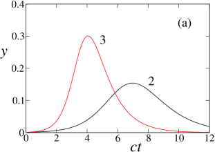
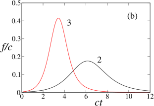
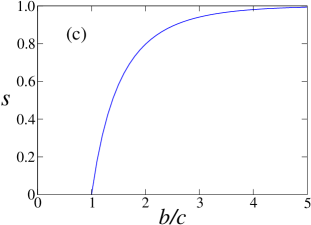
Figure 3: SIR model. (a) Fraction $y$ of infective individuals as a function of time $t$, for the values of $b/c$ indicated. (b) Epidemic curve, which is the frequency $f$ of new cases as a function of time $t$, for the values of $b/c$ indicated. (c) Order parameter $s$ versus the infection rate constant $b$. The order parameter is the area under the epidemic curve.

IV.2 SIR model

This model differs from the SIS model in an important feature. The infective individuals after healing acquires permanent immunization, meaning that they cannot be infected again. Therefore, in addition to susceptible (S) and infective (I) individuals, there are the immune individuals, which we call recovered (R). The model consists of two processes. The first is the infection, represented by

$${\rm S}\stackrel{{\scriptstyle\rm I}}{{\longrightarrow}}{\rm I},$$ (31)

occurring with an infection rate constant $b$, and the second is the spontaneous recovery, represented by

$${\rm I}\longrightarrow{\rm R},$$ (32)

occurring with a recovery rate constant $c$, which is strictly positive.

Denoting by $x$, $y$ and $z$, the number of susceptible, infective, and recovered individuals, respectively, then according to the rule of mass action the evolution equation of these variables are

$$\frac{dx}{dt}=-bxy,$$ (33)

$$\frac{dy}{dt}=bxy-cy,$$ (34)

$$\frac{dz}{dt}=cy.$$ (35)

As the total number of infective, susceptible and recovered is constant, the fractions $x$, $y$, and $z$ are related by $x+y+z=1$, and the three differential equations are not all independent.

The differential equations (33), (34), and (35) were introduced by Kermack and McKendrick in their study of epidemic spreading, allowing them to show the spreading threshold theorem kermack1927 , which we show next.

One solution of the evolution equations is $x=1$, $y=0$ and $z=0$ which is the non-spreading state. To find the stability of this state, we consider small deviations from this solution. The equation for $y$ becomes

$$\frac{dy}{dt}=\alpha y,$$ (36)

where $\alpha=b-c$, whose solution is

$$y=y_{0}e^{\alpha t},$$ (37)

and $y_{0}$ is the value of $y$ at $t=0$. Therefore, if $\alpha>0$, that is, if $b>c$, the number of infective grows exponentially and the spreading of the disease occurs. If $\alpha<0$, $y$ decreases and the disease does not spread. The onset of the spreading occurs when $b=c$.

To solve the time evolution equations we take the ratio between equations (35) and (33) to reach the equation

$$\frac{dz}{dx}=-\frac{c}{bx},$$ (38)

which can be integrated,

$$z=-\frac{c}{b}\ln x.$$ (39)

The constant of integration was chosen by considering that at the initial times, there is no recovered individuals, $z=0$, and the number of infective is very small so that the we may consider the fraction of the susceptible to be equal to one, $x=1$. Replacing the result (39) into $x+y+z=1$ we find the following relation between $x$ and $y$,

$$y=1-x+\frac{c}{b}\ln x,$$ (40)

which replaced in (33) gives

$$\frac{dx}{dt}=-x(b-bx+c\ln x).$$ (41)

In the integral form it reads

$$t=-\int\frac{dx}{x(b-bx+c\ln x)}.$$ (42)

The integral can be solved numerically to get $x$ as a function of $t$, from which we find $y$ and $z$. Alternatively, these variables can be obtained by solving numerically the set of equations (33), (34), and (35). The result of $y$ as a function of $t$, for a small initial value of $y$ and $z=0$, is shown in figure 3a. Initially there is an exponentially growth, as determined by the equation (37), then $y$ reaches a maximum and then decreases with time and vanishes asymptotically. This property is a consequence of the fact that an infective individual that becomes healthy acquires immunity and cannot be infected again. For long times there will be no infective individuals but only the recovered individuals and the ones that did not have acquired the disease, the susceptible. The disease has become extinct.

The frequency of new cases is the rate of the process (31) and given by

$$f=bxy,$$ (43)

and for the SIR model it is also $f=-dx/dt$. In figure 3b we show $f$ as a function of time, the epidemic curve. It was obtained from the numerical solution of $x$ referred to above. As initially the fraction of infective is increasing exponentially so does the quantity $f$. The epidemic curve increases, attains a maximum and then decreases to the zero value. The area $s$ under the epidemic curve, which is a measure of the size of the epidemic, is the order parameter and will be determined next.

When $t\to\infty$, no infective is left, as we have already seen, because once an infective individual is healed, it acquires immunization and cannot be infected again. In other words, the infective becomes recovered and remains in this state forever. Thus when $t\to\infty$, $y\to 0$, and the final fraction of susceptible $x^{*}$ and the final fraction of recovered $z^{*}$ are related by $x^{*}+y^{*}=1$. Replacing $x^{*}=1-z^{*}$ in (39) we find

$$z^{*}=-\frac{c}{b}\ln(1-z^{*}).$$ (44)

We have seen above that $f=-dx/dt$. In we integrate this equation in time, we find the order parameter $s$, that is,

$$s=\int_{0}^{\infty}fdt=1-x^{*}=z^{*},$$ (45)

where we have taken into account that $x$ at the initial time is equal to one. Replacing the result $z^{*}=s$ in equation (44) we find the equation that determines the order parameter,

$$s=-\frac{c}{b}\ln(1-s).$$ (46)

In figure 3c we show $s$ as a function of the infection rate constant $b$. When $b\leq c$, $s=0$ meaning that the size of the epidemic is zero or that there is no spreading of the disease. When $b>c$, the disease spreads and the size of the disease increases as the infection rate constant increases. The equation (46) is transcendental but can be solved numerically. However, a solution can be written explicitly when $s$ is small, in which case we find

$$s=2\frac{b-c}{c}.$$ (47)

The reproduction number is given by (8). Using $dy/dt$, given by equation (34), and recalling that $f=bxy$, we find

$$R=\frac{b}{c}x.$$ (48)

The basic reproduction number is found by setting $x=1$,

$$R_{0}=\frac{b}{c}.$$ (49)

IV.3 SISR model

In the SIR model, whenever an infective individual becomes healed it acquires permanent immunity. Here we consider a modification of the SIR model in which an infective individual may become again susceptible tome2015L ; ruziska2017 . There are three processes. The first is the infection, represented by

$${\rm S}\stackrel{{\scriptstyle\rm I}}{{\longrightarrow}}{\rm I},$$ (50)

occurring with an infection rate constant $b$. The second is the spontaneous recovery, represented by

$${\rm I}\longrightarrow{\rm R},$$ (51)

occurring with a rate constant $c$, where R represents an individual with permanent immunization. The third is the spontaneous recovery without immunization, represented by

$${\rm I}\longrightarrow{\rm S},$$ (52)

occurring with a rate constant $a$. An individual recovers from the disease but does not acquire immunization, becoming susceptible again.

The equation for the fractions $x$, $y$, and $z$ of susceptible, infective and recovered individuals are

$$\frac{dx}{dt}=-bxy+ay,$$ (53)

$$\frac{dy}{dt}=bxy-cy-ay,$$ (54)

$$\frac{dz}{dt}=cy,$$ (55)

and again $x+y+z=1$.

One solution of these equations is $x=1$, $y=0$, and $z=0$ corresponding to the absence of epidemic spreading. For small values of $y$ and for $x$ near one, the equation for $y$ reads

$$\frac{dy}{dt}=\alpha y,$$ (56)

where $\alpha=b-c-a$. Therefore, if $b>c+a$ then the epidemic spreading sets in whereas if $b<c+a$ there is no spreading of the disease.

The ratio of the equations (55) and (53) gives

$$\frac{dz}{dx}=-\frac{c}{bx-a},$$ (57)

which can be integrated,

$$z=-\frac{c}{b}\ln\frac{bx-a}{b-a},$$ (58)

with the condition $bx\geq a$. The constant of integration was chosen by considering that at the initial times, $z=0$, $y$ is negligible so that we may take $y=0$ and $x=1$.

The frequency of new cases $f$ is given by the rate of the process (50) and is $f=bxy$. The plot of $f$ as a function of $t$, the epidemic curve, has a bell shape similar to that of the SIR model. To get the area under this curve, which is the order parameter $s$, we proceed as follows. By an appropriate combination of the evolution equations (53) and (55), we write

$$bxy=-\frac{dx}{dt}+\frac{a}{c}\frac{dz}{dt},$$ (59)

so that

$$f=-\frac{dx}{dt}+\frac{a}{c}\frac{dz}{dt}.$$ (60)

Integrating $f$ in time from zero to infinity, we get

$$s=1-x^{*}+\frac{a}{c}z^{*},$$ (61)

where we recall that at $t=0$, $x=1$ and $z=0$, and $x^{*}$ and $z^{*}$ are the final values of $x$ and $z$.

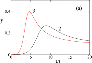
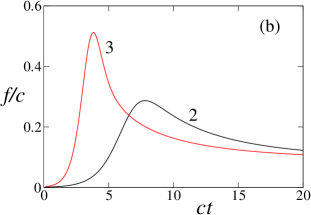
Figure 4: SIRI model. (a) Fraction $y$ of infective individuals as a function of time $t$, for $a/c=1.1$ and the values of $b/c$ indicated. The value of $y$ for long times is nonzero. (b) Epidemic curve, which is the frequency $f$ of new cases as a function of time $t$, for $a/c=1.1$ and the values of $b/c$ indicated. The asymptotic value of $f$ is nonzero. (c) Phase diagram in the plane $a/c$ versus $b/c$ showing the disease-free (DF), the endemic (ED) and the epidemic (EP) states.

To determine the value $z^{*}$, we observe that for long times $y$ vanishes and $x^{*}=1-z^{*}$. Replacing this result in the equation (58), we find the equation for $z^{*}$,

$$z^{*}=-\frac{c}{b}\ln\left(1-\frac{bz^{*}}{b-a}\right).$$ (62)

Using the relation (61) and the result $x^{*}=1-z^{*}$, we find $s=(c+a)z^{*}/c$ and the size of the epidemic $s$ is proportional to the final value of the fraction of the recovered $z^{*}$. The transcendental equation (62) can be solved when $z^{*}$ is small, with the result

$$z^{*}=\frac{2}{b}(b-a-c).$$ (63)

The threshold of the spreading of the disease occurs when $b=a+c$. If $b<a+c$ there will be no spreading and $s$ vanishes. However, if $b>a+c$, the disease will spread and for long times the fraction of the recovered individuals is $z^{*}$ given by equation (62).

The reproduction number is given by (8). Replacing $dy/dt$ given by equation (54) we find

$$R=\frac{b}{c+a}x.$$ (64)

The basic reproduction number is found by setting $x=1$,

$$R_{0}=\frac{b}{c+a}.$$ (65)

The numerical solution of the evolution equations give results for the fraction $y$ and for the frequency of new cases $f$ which are similar to those of the SIR model. Both these quantities grow exponentially, attain a maximum value and then decrease to their final zero values. The order parameter has also a similar behavior except that the critical point occurs when $b=c+a$.

IV.4 SIRI model

Here we consider another modification of the SIR model. In the SIR model, an individual that has been infected becomes immune, which means that a recovered individual remains forever in this condition. In the present modification the recovered individual loses the immunization and may be reinfected again tome2015L ; barros2017 . Therefore, to the two processes of the SIR model,

$${\rm S}\stackrel{{\scriptstyle\rm I}}{{\longrightarrow}}{\rm I},$$ (66)

occurring with an infection rate constant $b$, and

$${\rm I}\longrightarrow{\rm R},$$ (67)

occurring with a recovery rate constant $c$, we add the following process

$${\rm R}\stackrel{{\scriptstyle\rm I}}{{\longrightarrow}}{\rm I},$$ (68)

occurring with a reinfection rate constant $a$. The equation for the fractions of susceptible, infective, and recovered are

$$\frac{dx}{dt}=-bxy,$$ (69)

$$\frac{dy}{dt}=bxy-cy+ayz,$$ (70)

$$\frac{dz}{dt}=cy-ayz,$$ (71)

and we recall that $x+y+z=1$.

The frequency of new cases are determined by the processes (66) and (68) and is given by

$$f=bxy+ayz.$$ (72)

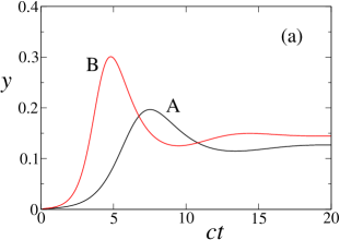
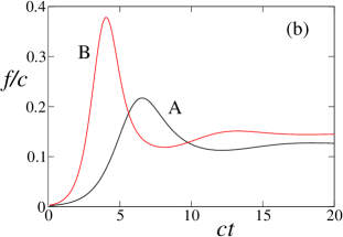
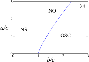
Figure 5: SIRS model. (a) Fraction $y$ of infective individuals as a function of time $t$. (b) Epidemic curve, which is the frequency $f$ of new cases as a function of time $t$. For the curve A: $a/c=1/3$ and $b/c=2$, and for the curve B: $a/c=0.3$ and $b/c=2.7$. (c) Phase diagram in the plane $a/c$ versus $b/c$ showing the non spreading(NS), the oscillation (OSC) and non-oscillating (NO) states.

One solution of the evolution equations is the trivial solution $x=1$, $y=0$, and $z=0$, which corresponds to the absence of spreading. For small values of $y$ and for $x$ near one, the equation for $y$ reads

$$\frac{dy}{dt}=\alpha y,$$ (73)

where $\alpha=b-c$. Therefore, if $b>c$ the epidemic spreads whereas if $b<c$ there is no spreading of the disease.

Dividing the equations (71) and (69) we find

$$\frac{dz}{c-az}=-\frac{dx}{bx},$$ (74)

which can be integrated to give

$$\ln\frac{c-az}{c}=\frac{a}{b}\ln x,$$ (75)

with the condition $az\leq c$. The constant of integration was found by assuming as we did before that at the initial time, $z=0$ and $x=1$.

For long times we have two types of solution. In one of them, the infected disappears, $y^{*}=0$, and there remain the recovered, $z^{*}\neq 0$, and the susceptible, $x^{*}\neq 0$. This solution occurs when $a\leq c$ and the asymptotic value $z^{*}$ is obtained by using (75) and replacing $x^{*}=1-z^{*}$. The result is the equation

$$\ln\frac{c-az^{*}}{c}=\frac{a}{b}\ln(1-z^{*}),$$ (76)

which should be solved for $z^{*}$. For small values of $z^{*}$ the solution is

$$z^{*}=2\frac{b-c}{c-a}.$$ (77)

The time dependent solution is similar to the solution of the SIR model.

As we have mentioned, $y^{*}=0$ for this solution so that the frequency of new cases $f$ vanishes for long times and the epidemic curve is also similar to that of the SIR model. The area $s$ under the epidemic curve is given by the integral

$$s=\int_{0}^{\infty}fdt,$$ (78)

which can be obtained from the solution of the evolution equations.

Let us consider the other solution, which is valid for $a>c$. The asymptotic values for this solution are $x^{*}=0$, $y^{*}=(a-c)/a$, and $z^{*}=c/a$, which are obtained by setting to zero the right-hand side of the evolution equations (69), (70), and (71). The time dependent solution leading to these values can be obtained by solving numerically the evolution equations. The fraction $y$ of infected is shown in figure 4a for the case $a/c=1.1$. From the solution for $x$, $y$ and $z$ we determine the frequency of new cases using (72), which is shown in figure 4b. This solution predicts a persistence of the disease because $f$ remains finite for long times.

The reproduction number is given by (8). Replacing $dy/dt$ given by equation (70) we find

$$R=\frac{bx+az}{c}.$$ (79)

The basic reproduction number is found by setting $x=1$, in which case $z=0$, and

$$R_{0}=\frac{b}{c}.$$ (80)

IV.5 SIRS model

We consider here a model with three classes of individuals like the SIR model: susceptible, infective and recovered. However, the present model consists of three instead of two processes tome2015L ; souza2010 . The first is the infection of susceptible individuals, represented by

$${\rm S}\stackrel{{\scriptstyle\rm I}}{{\longrightarrow}}{\rm I},$$ (81)

occurring with an infection rate constant $b$. The second is the spontaneous recovery, represented by

$${\rm I}\longrightarrow{\rm R},$$ (82)

occurring with a recovery rate constant $c$. These two processes are the same as the SIR model. In the present model, the recovered individuals are considered to have only partial immunity. Accordingly they may become again susceptible through an spontaneous process represented by

$${\rm R}\longrightarrow{\rm S},$$ (83)

occurring with a rate constant $a$.

The evolution equations for $x$, $y$, and $z$, the fractions of susceptible, infective and recovered individuals, are

$$\frac{dx}{dt}=-bxy+az,$$ (84)

$$\frac{dy}{dt}=bxy-cy,$$ (85)

$$\frac{dz}{dt}=cy-az.$$ (86)

Again $x+y+z=1$ and the equations are not all independent.

The trivial solution is $x=1$, $y=0$, and $z=0$, corresponding to the absence of spreading. Near this solution, that is, for small values of $y$ and for $x$ near 1, the equation for $y$ reads

$$\frac{dy}{dt}=\alpha y,$$ (87)

where $\alpha=b-c$. Therefore, if $b>c$ then $y$ increases exponentially and the spreading of the disease occurs. If $b<c$, it does not.

To determine the asymptotic fractions $x^{*}$, $y^{*}$, and $z^{*}$ of each class of individuals at long term we set to zero the right-hand sides of the equations (84), (85), and (86). The solution with a nonzero value of $y$ is

$$x^{*}=\frac{c}{b},\qquad y^{*}=\frac{a(b-c)}{b(a+c)},\qquad z^{*}=\frac{c(b-c)}{b(a+c)}.$$ (88)

The frequency of new cases $f$ is determined by the process (81) and is given by

$$f=bxy.$$ (89)

For long times it approaches a nonzero value given by

$$f^{*}=\frac{c^{2}(b-c)}{b(a+c)},$$ (90)

and in this respect it is like the SIS model, that is, the model predicts a persistence of the disease for long times, or that the disease becomes endemic. However for the present model the time dependence may present damped oscillations as shown in figure 5. This behavior is shown below.

Let us linearize the evolution equations (84) and (85) around the solution (88). To this end, we define the deviations $\xi=x-x^{*}$ and $\eta=y-y^{*}$ and write the evolution equations in these new variables. Up to linear terms in these variables, we find

$$\frac{d\xi}{dt}=M_{11}\xi+M_{12}\eta,$$ (91)

$$\frac{dy}{dt}=M_{21}\xi+M_{22}\eta,$$ (92)

where $M_{11}=-a(a+b)/(a+c)$, $M_{12}=-(a+c)$, $M_{21}=a(b-c)/(a+c)$, and $M_{22}=0$. The stability of the solution above is determined by the eigenvalues $\lambda$ of the matrix $M$ with elements $M_{ij}$ which are the roots of the equation

$$(a+c)\lambda^{2}+a(a+b)\lambda+a(b-c)(a+c)=0.$$ (93)

The product of the roots is positive and the sum of them is negative. If the roots are real then they are both negative and the solution is stable. Now, let us take a look at the complex roots which occurs when

$$a(a+b)^{2}\leq 4(b-c)(a+c)^{2}.$$ (94)

In this case we should look at the real part of $\lambda$. Since the real part is negative, then the solution is stable.

The conclusion is that the solution is stable but $x$, $y$, and $z$, and also $f$, will display damped time oscillations, as seen in figure 5, when the condition (94) is fulfilled. The values of $a$, $b$ and $c$ for this behavior is shown in figure 5c.

IV.6 SEIR model

In some infection diseases, the individual that has been infected takes a certain time to be infective. To take into account the latent period of such a disease, we introduce a class of individual called exposed (E) who has been infected but is not infective, but eventually becomes infective. A model that includes the exposed individuals is similar to the SIR, but the directed infection is replaced by the following two processes. The first is represented by

$${\rm S}\stackrel{{\scriptstyle\rm I}}{{\longrightarrow}}{\rm E},$$ (95)

occurring with an infection rate constant $b$, and the second is represented by

$${\rm E}\longrightarrow{\rm I}$$ (96)

occurring with a latent rate constant $h$, the inverse of which is a measure of the latent period of the exposed individual. The recover of an infective is the same as the SIR model, represented by

$${\rm I}\longrightarrow{\rm R},$$ (97)

occurring with a recovery rate constant $c$. The evolution equations for the fractions $x$, $u$, $y$, and $z$, of susceptible, exposed, infective and recovered, respectively, are

$$\frac{dx}{dt}=-bxy,$$ (98)

$$\frac{du}{dt}=bxy-hu,$$ (99)

$$\frac{dy}{dt}=hu-cy,$$ (100)

$$\frac{dz}{dt}=cy.$$ (101)

These equations are not all independent because $x+u+y+z=1$. These equations were introduced by Dietz to account for the latent period of infection dietz1976 .

The frequency of new cases $f$ is determined by the process (95) and is given by

$$f=bxy.$$ (102)

Considering that $bxy=-dx/dt$, it follows that the area under the epidemic curve is

$$s=\int_{0}^{\infty}fdt=1-x^{*},$$ (103)

where we have considered that at the initial times $x=1$.

The trivial solution of the equations (98), (99), (100), and (101) is $y=0$, $u=0$ and $x+z=1$. To determine the stability of this solution, we linearize the equation around the solution $y=0$, $u=0$, $z=0$ and $x=1$. The equation for $u$ and $y$ become

$$\frac{du}{dt}=by-hu,$$ (104)

$$\frac{dy}{dt}=hu-cy.$$ (105)

To find the solution of these equations we assume that

$$u=u_{0}e^{\alpha t}\qquad y=y_{0}e^{\alpha t}.$$ (106)

Replacing this solution in the equations of evolution we find

$$-hu_{0}+by_{0}=\alpha u_{0},$$ (107)

$$hu_{0}-cy_{0}=\alpha y_{0},$$ (108)

which are understood as a set of eigenvalue equations where $\alpha$ is understood as the eigenvalue. The possible values for $\alpha$ are the roots of

$$\alpha^{2}+(h+c)\alpha+h(c-b)=0,$$ (109)

the largest one being

$$\alpha=\frac{1}{2}\{-(h+c)+\sqrt{(h-c)^{2}+4hb}\}.$$ (110)

If $\alpha<0$, which occurs when $b<c$, the disease does not spread. If $\alpha>0$, which occurs when $b>c$, the disease spreads. In this regime, $y$ and $u$ grow exponentially with an exponent $\alpha$ given by equation (110). Let us compare this exponent with that of the SIR model, which is

$$\alpha_{\rm sir}=b-c.$$ (111)

In both cases the onset of spreading occurs when $b=c$. However, when $b>c$, that is, in the spreading regime, $\alpha<\alpha_{\rm sir}$ indicating that the epidemic growth rate is smaller for the SEIR model than it is for the SIR model. This is due to the necessary passage of an individual to the exposed state before reaching the infective state.

The behavior of the present model concerning the epidemic curve and the time behavior of fraction of infective is qualitatively similar to those of the SIR model shown in figure 3. The behavior of the size $s$ of the epidemic is the same as that of the SIR model and does not depend on the rate constant $h$ as we show in the following.

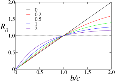
Figure 6: Basic reproduction number $R_{0}$ for the SEIR model as a function of the reduced infection rate $b/c$ for several values of the latent period $\ell=c/h$ of an exposed individual. Notice that, the SIR model corresponds to $\ell=0$. The outbreak of the epidemic occurs when $R_{0}=1$.

We divide the equation (101) by the equation (98)

$$\frac{dz}{dx}=-\frac{c}{bx},$$ (112)

which can be solved to give

$$z=-\frac{c}{b}\ln x,$$ (113)

where the constant of integration was found by considering that at the early stages, $z=0$ and $x=1$. For long times the infective as well as the exposed disappear, $y=0$ and $u=0$. Therefore, the sum of the final values $x^{*}$ and $z^{*}$ of the fractions of the susceptible and of the recovered equals one and $x^{*}=1-z^{*}$. Recalling that the order parameter $s=1-x^{*}=z^{*}$ we reach the following equation for $s$,

$$s=-\frac{c}{b}\ln(1-s)$$ (114)

which is identical to the equation (46) for the SIR model. It is worth mentioning that this equation says that $s$ does not depend on $h$ which means that the size of the epidemic is independent of $h$. In other terms, the presence of the exposed does not change the size of the epidemic. This process only slows the velocity of the spreading but not its size which is the same as that of the SIR model.

The reproduction number is given by (8). Replacing $dy/dt$ given by equation (100) we find

$$R=\frac{bx}{bx-h(u/y)+c}.$$ (115)

To find the basic reproduction number we need to know the ratio $u/y$ when $x=1$, that is, in the early stages of the spreading. According to (106), this ratio equals $u_{0}/y_{0}$ so that

$$R_{0}=\frac{b}{b-h(u_{0}/y_{0})+c}.$$ (116)

The ratio can be found from the eigenvalue equation (108). Dividing this equation by $y_{0}$ we find

$$h\frac{u_{0}}{y_{0}}-c=\alpha,$$ (117)

and $R_{0}$ acquires the form

$$R_{0}=\frac{b}{b-\alpha},$$ (118)

where $\alpha$ is the eigenvalue (110). A plot of $R_{0}$ is given in the figure 6 for various values of the latent period $\ell=c/h$. Notice that, the SIR corresponds to the case when the exposed rapidly becomes infective, that is, when the latent period is zero.

V The Ross theory of happenings

Ronald Ross received the Nobel Prize for Medicine in 1902 for his work on the transmission of malaria. He believed that it was not necessary to eliminate all mosquitoes to prevent the spreading of the disease but only to reduce the density of mosquitoes to a value below the critical level heesterbeek2015 . This conception as well as that of the threshold theorem of Kermack and McKendrick are understood as instances of the fundamental result of the statistical mechanics of interacting systems that the transition from one regime to another occurs only when one reaches a critical value of a parameter.

Ross advanced the idea of applying differential calculus to the dynamics of an infectious disease with the aim of its control and prevention. He even coined the name pathometry for what we call theoretical epidemiology. The theory introduced in his 1911 book on the prevention of malaria he called theory of happenings ross1911 . It is worth mentioning that the book contained the reports on the condition of malaria in several regions of the world, written by several authors. This includes the report by Oswaldo Cruz, the Brazilian epidemiologist, on the campaign on the prevention of malaria in southwest Brazil carried out in the first decade of the twentieth century.

His theory of happenings on the spreading of an infectious disease, Ross presented in an appendix to his book on the prevention of malaria of 1911 ross1911 and in subsequent papers ross1915 ; ross1916 , some of which with Hilda Hudson ross1917a ; ross1917b . In a population of $P$ individuals affected by a certain disease, the time variation $dZ/dt$ in the number of the affected $Z$ is $hA+qZ$ where $A=P-Z$ is the number of unaffected, $h$ is the proportion of unaffected that becomes affected and $q$ takes into account the demographic and recovery rates. For infectious diseases, Ross argues that $h$ is proportional to the fraction $x=Z/P$ of the affected, and writes $h=cx$ where $c$ is a constant which Ross calls the infection rate, and arrives at the following equation ross1911 ; ross1915 ; ross1916

$$\frac{dx}{dt}=cx(\ell-x).$$ (119)

The solution of this equation, given by Ross, is

$$x=\frac{x_{0}\ell}{x_{0}+(\ell-x_{0})e^{-c\ell t}},$$ (120)

revealing that $x$ increases slowly at the beginning and then very rapidly until it reaches an inflexion, and after that approaches the limiting value $\ell$ ross1915 ; ross1916 . According to Ross the current proportion of new cases to the total population is ross1915 ; ross1916

$$f=cx(1-x).$$ (121)

The equation (119) and its solution (120) are identical to the equations (15) and (21), respectively, and the frequency of new cases (121) is identical to $f$ given by (25). These results shows that the model considered by Ross is identified with the SIS model that we have analyzed.

VI Conclusion

We have presented an analysis of deterministic models for epidemic spreading. The equations were set up by using the analogy between chemical reactions and the processes occurring in the epidemic spreading which are understood as a change of the class of an individual. The main analogy was the use of the law of mass action, which provides the rate of the several processes that define an epidemic model. We have also emphasized the analogy of the onset of an epidemic with a thermodynamic phase transition. When the infection constant changes it reaches a critical value at which the spreading takes place. The infection constant is argued to depend on the density of the population and as it increases the spreading outbreaks at a certain critical density, which is the theorem advanced by Kermack and McKendrick.

We have also analyzed the quantities that characterizes the spreading of an epidemic. One of them is the frequency of new cases, which is the number of new infected individuals per unit time. When this quantity vanishes the epidemic comes to an end. In this case the area of the epidemic curve is a measure of the epidemic and may be identified as the order parameter. It may happen that the frequency of new cases does not vanishes and in this case the disease becomes endemic. We have seen that the SIRS model which is appropriate for this case, predict oscillations in the frequency of new cases.

Another way of determining the outbreak of the spreading is by means of the stability analysis of the disease-free state which is the state without any infective individuals. Any model of spreading must have this state which in stochastic models is called absorbing state. The stability analysis gives the behavior of the spreading at the beginning and shows that the growth of the epidemic is exponential. We have related the growth exponent with the basic reproduction number. When the exponent change signs, which means that the reproduction number passes from a value less than one to a value greater than one, the spreading outbreaks.

All the properties were obtained by solving the evolutions equations, which are ordinary differential equations of first order in time. This may be obtained in closed form or by numerical methods. We have finally showed that the SIS model was in fact the model originally studies by Ross in his theory of happenings.

Appendix A Law of mass action

The law of mass action tome2015L was formulated originally by Guldberg and Waage in the context of the equilibrium of chemical reactions waage1864a ; waage1864b ; guldberg1864 . Since then it was used in the chemical kinetic theory and in other fields such as that of the present application.

Let us consider a set of chemical reaction represented by

$$\sum_{i({\rm reac.})}\nu_{ij}A_{i}\,\,\to\!\!\sum_{i({\rm prod.})}\nu_{ij}^{\prime}A_{i},$$ (122)

where $A_{i}$ represents a molecule of the $i$ species and $\nu_{ij}\geq 0$ and $\nu_{ij}^{\prime}\geq 0$ are the stoichiometric coefficients related to the $j$-th reaction. The sum on the left-hand side is over the reactants whereas that on the right is over the products of the reaction. A catalytic reaction is understood as a reaction where a certain molecule $A_{i}$ appears both as a reactant and as a product of the reaction, with the same stoichiometric coefficient, $\nu_{i}^{\prime}=\nu_{i}>0$, and an auto-catalytic, if $\nu_{i}^{\prime}>\nu_{i}>0$.

Let us denote by $\rho_{i}$ the concentration of molecules of species $A_{i}$, which is the number of molecules per unit volume. The evolution equation for $\rho_{i}$ is postulated to be of the form

$$\frac{d\rho_{i}}{dt}=\sum_{j}(\nu_{ij}^{\prime}-\nu_{ij})g_{j},$$ (123)

which is a sum of terms, one for each one of the reactions in which the molecule $A_{i}$ appears as a reactant or as a product of the reaction. According to the law of mass action, the term $g_{j}$ is given by

$$g_{j}=k_{j}^{*}\prod_{i}(\rho_{i})^{\nu_{ij}},$$ (124)

where $k_{j}^{*}$ is the intrinsic reaction rate constant related to the $j$-th reaction, and the mathematical product in $i$ is over the reactants.

Suppose we wish to formulate the equations above in terms of the fraction $x_{i}$ of each species. If we denote by $N$ the total number of molecules then the relation between density and fractions is $Nx_{i}=V\rho_{i}$ because each one of these two terms equals the number of molecules of species $i$. Defining $\gamma=N/V$ this relation can be written as

$$\rho_{i}=\gamma x_{i}.$$ (125)

From now on we consider that $N$, or equivalently $\gamma$, is invariant in time, or that it varies so slowly compared to the variation of the fractions $x_{i}$, that it might be taken as constant in time. With this condition in mind, we replace (125) in (123) to find the evolution equation in terms of the fractions,

$$\frac{dx_{i}}{dt}=\sum_{j}(\nu_{ij}^{\prime}-\nu_{ij})f_{j},$$ (126)

where $f_{j}$ is

$$f_{j}=k_{j}\prod_{i}(x_{i})^{\nu_{ij}},$$ (127)

and the mathematical product in $i$ is again over the reactants. The reaction rate constant $k_{j}$ is proportional to the intrinsic reaction rate constant $k_{j}^{*}$ and related to $\gamma$ by

$$k_{j}=k_{j}^{*}\gamma^{-1}\prod_{i}\gamma^{\,\nu_{ij}}.$$ (128)

Let us consider the spontaneous reaction

$${\rm A}_{1}\longrightarrow{\rm A}_{2}.$$ (129)

The rate constant $k$ of this reaction is identical to the intrinsic rate constance $k^{*}$, that is, $k=k^{*}$. However, for the auto-catalytic reaction

$${\rm A}_{1}+{\rm A}_{2}\longrightarrow{\rm A}_{1}+{\rm A}_{3},$$ (130)

the rate constant $k$, according to the formula (128), is $\gamma$ times the intrinsic rate constant $k^{*}$, that is, $k=\gamma k^{*}$.

The distinction between a rate constant and an intrinsic rate constant is that the intrinsic is free from concentration dependence whereas the rate constant may depend on the concentration as shown in the second example above.

References

- (1) N. T. J. Bailey, The Mathematical Theory of Epidemics, Hafner, New York, 1957.
- (2) R. M. Anderson and R. M. May, Infectious Diseases of Humans, Oxford University Press, Oxford, 1991.
- (3) E. Renshaw, Modelling Biological Population in Space and Time, Cambridge University Press, Cambridge, 1991.
- (4) D. Mollison (ed.), Epidemic Models, Cambridge University Press, Cambridge, 1995.
- (5) A. Hastings, Population Dynamics, Springer, New York, 1997.
- (6) M. J. Keeling and P. Rohani, Modeling Infectious Diseases, Princeton University Press, Princeton, 2008.
- (7) R. Ross, The Prevention of Malaria, Murray, London, 1911.
- (8) W. O. Kermack and A. G. McKendrick, Proc. R. Soc. A 115, 700 (1927).
- (9) H. E. Soper, J. R. Stat. Soc. 92, 34 (1929).
- (10) G. Macdonald, Trop. Dis. Bull. 49, 813 (1952).
- (11) J. A. P. Heesterbeek and M. G. Roberts, Phil. Trans. R. Soc. B 370, 20140307 (2015).
- (12) J. A. P. Heesterbeek, Acta Biotheoretica 50, 189 (2002).
- (13) M. S. Bartlett, J. R. Stat. Soc. B 11, 211 (1949).
- (14) N. T. Bailey, Biometrika 40, 177 (1953).
- (15) P. Wittle, Biometrika 42, 116 (1955).
- (16) R. M. Nisbet and W. C. S. Gurney, Modelling Fluctuating Populations, Blackburn, Caldwell, 1982.
- (17) T. Tomé and M. J. de Oliveira, Stochastic Dynamics and Irreversibility, Springer, Heidelberg, 2015.
- (18) T. E. Harris, Ann. Probab. 2, 969 (1974).
- (19) P. Grassberger, Math. Biosci. 62, 157 (1983).
- (20) P. Grassberger and A. de La Torre, Ann. Phys. 122, 373 (1983).
- (21) T. Ohtsuki and T. Keyes, Phys. Rev. A 33, 1223 (1986).
- (22) J. Satulovsky and T. Tomé, Phys. Rev. E 49, 5073 (1994).
- (23) R. Durrett, in D. Mollison (ed.), Epidemic Models, Cambridge University Press, Cambridge, 1995; p. 187.
- (24) T. Antal, M. Droz, A. Lipowski, and G. Ódor Phys. Rev. E 64, 036118 (2001).
- (25) S. M. Dammer and H. Hinrichsen, Phys. Rev. E 68, 016114 (2003).
- (26) D. R. de Souza and T. Tomé, Physica A 389, 1142 (2010).
- (27) T. Tomé and M. J. de Oliveira J. Phys. A 44, 095005 (2011).
- (28) D. R. de Souza, T. Tomé, S. T. R. Pinho, F. R. Barreto, and M. J. de Oliveira, Physical Review E 87, 012709 (2013).
- (29) A. H. O. Wada, T. Tomé, and M. J. de Oliveira, J. Stat. Mech. P04014 (2015).
- (30) F. M. Ruziska, T. Tomé, M. J. de Oliveira, Physica 467, 21 (2017).
- (31) T. Tomé and M. J. de Oliveira, Phys. Rev. E 79, 061128 (2009).
- (32) A. T. C. Silva, V. R. V. Assis, S. T. R. Pinho, T. Tomé, and M. J. de Oliveira, Physica A 468, 131 (2017).
- (33) A. G. Dickman, R. Dickman, and F. A. Barbosa, Rev. Bras. Ens. Fis. 28, 23 (2006).
- (34) M. N. Burattini, M. Chen, A. Chow, F. A. B. Coutinho, K. T. Goh, L. F. Lopez, S. Ma, and E. Massad, Epidemiol. Infect. 136, 309 (2008).
- (35) S. T. R. Pinho, C. P. Ferreira, L. Esteva, F. R. Barreto, V. C. Morato e Silva, and M. G. L. Teixeira, Phil. Trans. R. Soc. A 368, 5679 (2010).
- (36) K. Dietz, in J. Berger, W. J. Bühler, R. Repges, and P. Tautu (eds), Mathematical Models in Medicine, Springer, Berlin, 1976.
- (37) J. Marro and R. Dickman, Nonequilibrium Phase Transitions in Lattice Models, Cambridge University Press, Cambridge, 1999.
- (38) M. Henkel, H. Hinrichsen, and S. Lübeck, Non-Equuilibrium Phase Transitions, Vol. 1, Springer, Dordrecht, 2008.
- (39) F. L. Ribeiro, Rev. Bras. Ens. Fis. 39, e1311 (2017).
- (40) J. A. R. Cunha, L. Cândido, F. A. Oliveira, e A. L. A. Penna, Rev. Bras. Ens. Fis. 39, e3303 (2017).
- (41) A. S. Barros and S. T. R. Pinho, Phys. Rev. E 95, 062135 (2017).
- (42) R. Ross, Brit. Med. J. 1, 546 (1915).
- (43) R. Ross, Proc. R. Soc. A 92, 204 (1916).
- (44) R. Ross and H. P. Hudson, Proc. R. Soc. A 93, 212 (1917).
- (45) R. Ross and H. P. Hudson, Proc. R. Soc. A 93, 225 (1917).
- (46) P. Waage, C. M. Guldberg, Forhandlinger I Videnskabs-selskabet I Christiania, 35 (1964).
- (47) P. Waage, Forhandlinger I Videnskabs-selskabet I Christiania, 92 (1964).
- (48) P. C. M. Guldberg, Forhandlinger I Videnskabs-selskabet I Christiania, 111 (1964).