Charged surfaces and slabs in periodic boundary conditions

Abstract

Plane wave density functional theory codes generally assume periodicity in all three dimensions. This causes difficulties when studying charged systems, for instance energies per unit cell become infinite, and, even after being renormalised by the introduction of a uniform neutralising background, are very slow to converge with cell size. The periodicity introduces spurious electric fields which decay slowly with cell size and which also slow the convergence of other properties relating to the ground state charge density. This paper presents a simple self-consistent technique for producing rapid convergence of both energies and charge distribution in the particular geometry of 2D periodicity, as used for studying surfaces.

1 Introduction

Plane-wave electronic structure codes generally enforce periodicity in all three dimensions, and this periodicity applies not just to the structure, but also to the calculated potential. Whilst neutral bulk crystals have this periodicity, systems such as surfaces and slabs are of lower dimensionality. To study these systems in such codes, a region of vacuum is used to separate the system from its fictitious periodic images. As the extent of the vacuum is increased, in many cases properties converge to the values that they would have in the absence of the imposed periodicity. This convergence is often slow, so corrections to accelerate the convergence have been derived for various geometries[1]. However, in the particular case of a charged 2D system, the energy does not converge, but increases linearly with vacuum extent.

Charged 2D systems are of interest in many areas, and have been the subject of both experiment and of Density Functional Theory (DFT) calculations. An inexhaustive list, with references to some recent work, would include exfoliation [2, 3], adsorption of gas molecules on surfaces[4, 5], and phase transitions in thin sheets[6]. In all of these areas there is a desire to study the effect of varying charge on the process, and a need to resolve small energy differences accurately.

Various methods have been proposed for addressing the issues which arise, including the use of a 2D Ewald summation in place of the usual 3D Ewald summation[7], truncated Coulomb methods[8, 9], extrapolation[10, 11], minimum image Coulomb potentials[9, 12] and Green’s function approaches[13, 14, 15]. Some of these techniques bring their own constraints, such as the Coulomb truncation methods which require the extent of the vacuum region to be greater than the extent of the non-vacuum region[16]. In this paper a simple correction is described which can be applied to any code which uses the standard 3D Ewald summation, and which greatly accelerates the convergence of the energy other properties of the wavefunction with vacuum size in charged systems.

When computing charged systems using periodic boundary conditions, the periodicity causes an extra, unphysical electric field to arise, and this perturbs the charge density from what it would have been in the aperiodic case[17]. This is most noticeable if the system is highly polarisable, for example, a metal. That the charge density is significantly perturbed from the aperiodic ground state means that simple post hoc corrections will not be highly accurate as they will be unable to correct the charge density, although more sophisticated post hoc schemes which estimate the value of $\epsilon_{r}$ can improve this[18, 19]. The problem is not confined to plane-wave codes, for other codes also find it convenient to use methods which force the potential to be periodic, and thus require corrections when modelling systems in which it should be aperiodic[9, 20].

This paper discusses post hoc corrections which merely correct the energy, but not forces or density-dependent properties, and it also introduces a self-consistent correction which not only gives a superior correction to the energy and could be used to correct forces, but the self-consistent correction also corrects the density and thus improves the convergence of density-dependent properties.

2 Theory

A sheet carrying a uniform charge per unit area of $\sigma$ produces an electric field on each side of magnitude $0.5\sigma/\epsilon_{0}$, assuming symmetric boundary conditions.

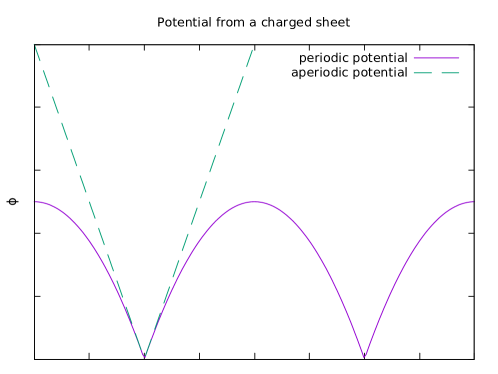
Figure 1: The potential arising from a uniformly charged sheet with and without periodic boundary conditions. Two repeat units are show in the periodic case.

When such a sheet is modelled in a standard plane wave code, with periodicity in all three dimensions imposed, the resulting potential is as shown in figure 1. In the vacuum region where the aperiodic system correctly has a constant field and a linear potential, the periodic system has a linear field and a quadratic potential. This can be understood as arising from the uniform compensating charge placed throughout the cell, usually referred to as ‘jellium’.

The method generally used in plane wave codes of dividing the electrostatic interaction into the three parts of ion-ion, electron-electron and ion-electron results in three infinite terms. However, if the $g=0$ reciprocal space component of the charge density is removed from each of these, not only do they become finite, but the three removed terms cancel exactly for an uncharged system. So the sum is always performed with the assumption that the total ionic and electronic charges are equal. If the original total charges were not equal, as would be the case in a charged system, then within the calculation the total charges are treated as equal. This is done, implicitly, by ignoring the $g=0$ components of the densities, which is equivalent to adding a uniform compensating charge to the system to make it neutral[21].

As can be seen from figure 1, in the immediate vicinity of the sheet, the potential and field is the same in the periodic and aperiodic cases. However, in the periodic case the field falls below the aperiodic value in a linear fashion with increasing distance from the sheet.

If, instead of a thin sheet, the charged body is a conducting slab of significant thickness, the situation changes to that shown in figure 2.

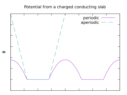
Figure 2: The potential arising from a uniformly charged conducting slab with and without periodic boundary conditions. The thickness of the slab is 40% of the periodic repeat distance in the direction normal to the slab.

In this case, in the aperiodic case, the charge rests solely on each surface of the slab, giving there a charge density of $0.5\sigma$, and the field strength is as before. Within the conducting slab the potential must be constant.

In the periodic case for the charged conducting slab, again the potential within the conducting slab must be constant, and in the vacuum region the quadratic term must be the same as for the thin charged sheet, as the density of the jellium does not depend on the thickness of the slab. If $z$ is the axis perpendicular to the slab, then the electrostatic potential, $\phi$, is a function of $z$ only, and, in the vacuum region $d^{2}\phi/dz^{2}=\rho_{j}/\epsilon_{0}$ where $\rho_{j}$ is the charge density due to the neutralising jellium. In this case the surface charge density on each side of the slab is no longer $0.5\sigma$. It is reduced because some of the excess charge of the slab must move to neutralise the jellium charge in the slab region where the potential must be constant, and hence the total charge density, including the jellium, must be zero. Thus the surface charge density is reduced by a factor of the width of the vacuum region divided by the periodic distance normal to the surface. The surface field is reduced by the same factor.

2.1 Post hoc energy corrections

If one considers a charged sheet, placed at the origin, then, in the periodic case, the potential as a function of $z$ is

$$\phi=\frac{q}{2\epsilon_{0}A}|z|-\frac{q}{2\epsilon_{0}V}z^{2}-\frac{qc}{12\epsilon_{0}A}$$ (1)

where $A$ is the cell’s area in the plane of the slab, $c$ the repeat distance perpendicular to the slab, $V=Ac$ its volume, and $q$ the charge per unit cell of the sheet. The constant term arises because codes set the average electrostatic potential (the reciprocal space $g=0$ term) to zero. The energy of the sheet in this potential is just $0.5q\phi(0)$, the factor of a half avoiding the double-counting associated with the sheet being in the potential which it itself has produced, which is

$$U=-\frac{q^{2}c}{24\epsilon_{0}A}$$ (2)

This term is linear in $c$, the cell length normal to the slab, and so is best removed by extrapolating $c$ to zero.

This expression can also be derived by integrating the energy density of the electric field, $0.5\epsilon_{0}E^{2}$. In the half of the cell from $z=0$ to $z=c/2$ the field, $E$, is given by differentiating equation 1,

$$E(z)=\frac{q}{2\epsilon_{0}A}-\frac{qz}{\epsilon_{0}V}$$ (3)

and then, considering the total contribution from the two equivalent half cells,

$$U=2\int_{0}^{\frac{c}{2}}0.5\epsilon_{0}E^{2}\,A\,dz$$ (4)

which results in the same expression for the energy.

To find the next order term in the post hoc correction to the energy, consider splitting the thin charged sheet above into two sheets, each of charge $q/2$, and separated by a distance $2d$. There is an energy term which represents moving the charge up the linear term of the ‘V’-shaped potential. However, as this linear part of the potential is independent of $c$, so too is this energy, and, as a constant offset in the energy, it can be ignored.

There is a contribution to the energy arising from the quadratic term in equation 1. This is

$$U=-\frac{q^{2}}{4\epsilon_{0}V}d^{2}$$ (5)

with again a factor of two from double-counting[22]. Furthermore there is an energy arising because the average of the potential has now changed, so the constant term in equation 1 has to change to keep the average potential zero. To first order, this requires an extra constant term of $qd^{2}/(2\epsilon_{0}V)$. With the usual comments about overcounting, this gives rise to a second contribution to the energy, identical in form and sign to equation 5. If one further defines a quadrupole moment $Q_{cc}=qd^{2}$, then the total post hoc energy correction is

$$U=-\frac{q^{2}c}{24\epsilon_{0}A}-\frac{qQ_{cc}}{2\epsilon_{0}V}$$ (6)

2.2 Self consistent corrections

In order to produce results which converge rapidly with vacuum size, it is necessary to ensure that fields and charge distributions in and near the slab are independent of the width of the vacuum region. This can be achieved by adding a correcting potential which removes the quadratic potential introduced by the jellium. Such a potential will have a discontinuity in its derivative in the middle of the vacuum region, and can be considered to represent a compensating charged sheet, of charge density $-\sigma$, in the middle of the vacuum region. It is thus similar to the method of Lozovoi and Alavi[23] who used a Gaussian-smeared sheet in the centre of the vacuum region. When considered as a compensating charge, the net charge of the cell becomes zero, and no jellium is introduced into the system. In order to achieve this, the potential which has to be added is

$$\phi_{\textrm{corr}}=\frac{qz^{2}}{2\epsilon_{0}V}-\frac{qc^{2}}{24\epsilon_{0}V}$$ (7)

which will result in a total electrostatic potential of

$$\phi_{\textrm{tot}}=\frac{qc|z|}{2\epsilon_{0}V}-\frac{qc^{2}}{8\epsilon_{0}V}$$ (8)

which is identical to the electrostatic potential for the aperiodic case in figure 1.

Introducing this correction to the potential results in an additional energy correction of

$$U=-\frac{q^{2}c}{12\epsilon_{0}A}$$ (9)

This arises from noting that this potential arising from the fictitious charged sheet will be allowed to act on the electrons and ions, but to include all the energy terms of the system including the charged sheet, the extra potential must also be allowed to act on the sheet itself, subject to a factor of a half to avoid double counting. The charged sheet is placed at $z=c/2$, at which point the value of $\phi$ as given by equation 7 is

$$\phi_{\textrm{corr}}(\frac{c}{2})=\frac{qc^{2}}{12\epsilon_{0}V}$$ (10)

This gives an extra energy term of

$$U=\frac{q^{2}c}{24\epsilon_{0}A}$$ (11)

There remains one final correction to the energy. As the vacuum region is expanded, the energy of the cell will increase due to the energy density of the electric field in the vacuum. The field remains constant with increasing vacuum size, but its volume increases. This argument gave equation 4, but, whereas in the case of the post hoc correction the field was given by equation 3, in the self-consistent case the field is now simply $\sigma/2\epsilon_{0}$ or $q/2\epsilon_{0}A$, as the field is now identical to what it would be in the aperiodic system. So after the self consistent correction the integral evaluates to $q^{2}c/(8\epsilon_{0}A)$. This is not an energy term that is desired in the final result, so it must be subtracted, and the term from equation 11 added. Thus the total correction is

$$U=-\frac{q^{2}c}{12\epsilon_{0}A}$$ (12)

as stated in equation 9.

This energy can either be included explicitly, or by adding a constant to equation 7. The latter approach has the effect of changing the sign of the constant term in that equation.

3 Non-uniform systems

The above theory has been developed by considering uniformly-charged sheets. A real surface does not have a uniform charge density or potential, though it can be shown that the long-range effects of non-uniformity in either the charge density or the potential decay rapidly with increasing vacuum extent.

Consider an isolated thin sheet with a non-uniform charge distribution such that the potential close to its surface is sinusoidal in the plane of the sheet. In the vacuum region, Gauss’s Law states that the potential must obey $\nabla^{2}\phi=0$. Choosing $x$ to be the direction of sinusoidal variation, the solution is

$$\phi = a\exp(ikx-kz)+bz+c$$ (13)

$$\nabla^{2}\phi = a(-k^{2}+k^{2})\exp(ikx-kz)=0$$ (14)

So any Fourier component of $\phi$ parallel to the slab decays exponentially away from it (discounting the unphysical mathematical possibility of an exponential increase). An arbitrary 2D-periodic charge density on a sheet can be considered as the sum of Fourier components, each of which must decay exponentially in the vacuum region. The slowest-decaying component will be that with the smallest $k$ value, i.e the longest wavelength. As $\phi$ must have the periodicity of the unit cell, its periodic part will decay in the vacuum region at least as fast as $\exp(-2\pi z/a)$ where $a$ is the longer of the two cell axes in the plane of the slab. And as the potential mediates the interaction between the system’s periodic images, the difference between the interactions from a uniformly charged slab, and a periodically charged one, will decay similarly with increasing vacuum extent. This confirms statements based on numerical observations about the required vacuum extent for well-converged calculations[7].

4 Non-symmetric systems

The systems considered so far all have sufficient symmetry to cause their dipole moment to be zero about the centre of the slab. However, the theoretical approach presented in this paper is readily generalisable to systems lacking this symmetry. In a charged system it is possible to pick an origin about which the dipole moment is zero, and then this self-consistent correction can be applied centred on this origin[1].

A shift to the point about which the dipole moment is zero requires a shift of $p/q$, where $p$ is the dipole moment and $q$ the net charge. Applying this shift to equation 7 leads to the emergence of a linear term in the potential, $pz/\epsilon_{0}V$. This is the expected correction for the dipole-dipole interaction between uncharged slabs as given by Neugebauer and Scheffler[24], showing an equivalence between shifting co-ordinates to eliminate the dipole moment, and explicitly including it.

This generalisation enables a correction to the forces on the ions to be obtained by differentiating the energy correction with respect to the ionic positions, although this extension is not further discussed here.

5 Validation calculations

To verify the theory presented above, calculations were performed on a system comprising of a varying number of graphene sheets stacked in the ABAB sequence. These systems are metallic. A calculation was also performed on a non-metallic system which lacks inversion symmetry, a slab of SiC. No atomic relaxation was performed in these calculations, as only the electronic minimisation was of interest. In the graphene calculations the in-plane lattice parameter was set to 2.46Å, and for SiC to 3.08Å.

Firstly results are presented for a single layer of graphene, with a charge of +2e per unit cell (pair of atoms). This system acts as a thin, charged sheet. Secondly results are presented for a four layer system of graphene, again with a charge of +2e per unit cell. This system acts as a charged conducting slab, with the graphene occupying the majority of the cell when the vacuum separation is small. Finally results are presented for a thin slab of SiC, cut along its $\{$0001$\}$ planes, as an example of a system which lacks inversion symmetry.

The calculations were all performed with a high cutoff of 550eV, as the positive charge tends to make orbitals more compact requiring a larger basis set, and using the Francis-Payne correction for a finite basis set[25]. The validity of the corrections presented will not depend on the exchange-correlation functional used, so these calculations used the computationally-inexpensive LDA.

The Castep[26] code was used for all the calculations. The post hoc corrections were performed using a modified version of c2x[27], whereas the self consistent corrections used a version of Castep modified for this purpose.

As well as considering the convergence of the total energy, the convergence of one component of the quadrupole moment is also considered, the same component which appears in the post hoc energy correction, equation 6. The convergence of this moment is another measure of how well converged the electron density is, and is a property which is not readily corrected by post hoc methods. This is calculated in the direction perpendicular to the slab, after averaging over the two orthogonal directions, as

$$Q_{cc}=\int_{0}^{c}(z-0.5c)^{2}\rho(z)\,dz$$ (15)

Where $c$ is the extent of the cell in the $z$ direction perpendicular to the slab, and $\rho(z)$ the total charge density after averaging over the directions parallel to the slab. The slab is centred at $z=c/2$ with $z=0$ (or $z=c$) being the centre of the vacuum region.

5.1 Single Layer of Graphene

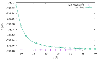
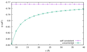
Figure 3: The energy (left) and quadrupole moment (right) from a single layer of graphene with a charge of +2e per unit cell (2 atoms) as the cell length (vacuum separation) is varied. For the energy a post hoc correction is shown as well as a self-consistent correction. For the quadrupole, no post hoc correction was applied.

A single layer of positively-charged graphene is well modelled by a thin sheet of charge. With a charge of +1e per atom, the $\pi$ orbitals will be unoccupied, and the charge density is close to two dimensional. The post hoc corrections, which would be exact if the change in the field caused by the periodicity did not cause a change in the charge distribution, should therefore be quite good.

Figure 3 shows the convergence of the energy, after the post hoc correction, and also the convergence of the quadrupole moment. Both are compared to calculations with a self-consistent correction.

No post hoc correction can be applied to the quadrupole moment without extra information such as the thickness and polarisability of the system. The geometry of the system is such that the variation of the quadrupole moment is not great, but the application of the self-consistent correction gives a very constant value. The variation of the quadrupole moment with the self-consistent correction shows no obvious trend, just random noise, as it varies between -0.77309 and -0.77318 eŲ. With a cell length of just 8Å both the quadrupole moment, and the energy, are converged in the self-consistent case.

5.2 Four Layers of Graphene

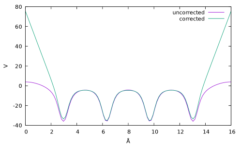
Figure 4: The potential arising from four layers of graphene, with a charge of +2e per unit cell (8 atoms). A standard uncorrected DFT calculation is shown, along with the potential after the correction discussed in this paper. The uncorrected potential has been shifted to align the two potentials in the centre of the slab.

Four layers of graphene were stacked in an ABAB sequence with a 3.36Å layer separation. The total extent of the slab is therefore approximately 13.5Å. Calculations were performed with the repeat distance perpendicular to the slab varying from 16Å to 40Å in 2Å steps. Figure 4 shows the potential averaged over planes parallel to the slab when the repeat distance is 16Å in both the uncorrected case, and after applying the self-consistent correction of equation 7.

If one ignores the oscillations in the potential within the slab itself, this figure looks similar to figure 2. The field at the slab’s surface is considerably suppressed in the uncorrected calculation, and this will alter the surface properties.

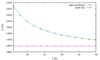
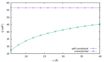
Figure 5: The energy (left) and quadrupole moment (right) computed for four layers of graphene with a charge of +2e per unit cell (8 atoms) as the cell length (vacuum separation) is varied. For the energy a post hoc correction is shown as well as a self-consistent correction. For the quadrupole, no post hoc correction was applied.

Figure 5 shows the convergence of the energy of the four layer graphene system, after the post hoc correction, and also the convergence of the quadrupole moment, and is thus the four-layer equivalent of figure 3. The self-consistent correction still shows very good convergence with cell size. The post hoc energy correction and uncorrected quadrupole moment now show quite poor convergence. However, this is to be expected for the following reason.

If one models the graphene slab as simply a conductor of thickness $2L$ and charge $2q$, then, in the absence of periodicity, the charges will lie on the two surfaces, and the quadrupole moment will be $Q_{cc}=2qL^{2}$. Once periodicity is introduced, and with it its neutralising jellium, the surface charges are reduced by a factor of $1-\frac{2L}{c}$. It is hard to define precisely the thickness of a slab of just a few atomic layers, but the thickness measured between the surface nuclei is about 10Å. So when $c$ is 40Å, one would expect the quadrupole moment to have reached about three quarters of the value it would have when $c$ is infinity. The self-consistent calculation produces values for $Q_{cc}$ which vary randomly between 56.522 and 56.538 eŲ, whereas the non self consistent calculation gives $Q_{cc}$ as 45.226 eŲ at $c=$40Å. This is almost exactly 80% of the self-consistent value, but the simple theory of this paragraph which predicted 75% neglected the contribution to the quadrupole moment of the bulk material, and the setting of $2L=10$Å is an underestimate. Thus it can be seen that the quadrupole moment converges slowly with increasing vacuum separation in the absence of any self-consistent correction, but converges rapidly with the correction presented in this paper. For this system, it is well converged when the vacuum separation is still smaller than the slab thickness.

5.3 A Non-Symmetric System

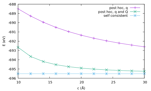
Figure 6: The energy from two layers of SiC with a charge of +2e per unit cell (4 atoms) as the cell length (vacuum separation) is varied. A simple post hoc correction depending just on the charge is shown, a post hoc correction including the quadrupole moment, and a self-consistent correction. The self-consistent line shows noise, and the variation between its greatest and least value is less than 0.5meV.

A slab of silicon carbide cut along its $\{$0001$\}$ planes lacks inversion symmetry and, if uncharged, will have a dipole moment perpendicular to the slab. For good convergence with cell size in the neutral system a self-consistent correction for this dipole moment is required[28]. In the following, two layers of a charged system are considered, again with an overall charge of +2e per unit cell. The distance between the planes of the centres of the nuclei at the two surfaces (carbon on one surface, silicon on the other) was just over 3.1Å.

Calculations were performed in the same manner as for the graphene sheets, save that the centre of the quadratic correcting potential was no longer fixed at the centre of the slab, but allowed to move self-consistently to the point about which the dipole moment of the charged system was zero.

Figure 6 shows the energy after removing the linear term using the post hoc correction of equation 2, the energy after using the better post hoc correction of equation 6 which includes consideration of the quadrupole moment $Q_{cc}$, and also the energy from the self-consistent calculation. The self-consistent energy shows no systematic variation with $c$ in this range, and the extent of the random variation is less than 0.5meV. Even when $c=30$Å, the better of the post hoc corrections is still about 0.25eV from the self-consistent result, showing that the self-consistent correction has again achieved convergence with respect to the width of the vacuum region at a much smaller cell size than the post hoc corrections.

6 Details of Implementation

Two details of the implementation of the self-consistent correction are worth comment. Firstly the systems chosen have a postive charge. Care must be taken when working with negatively-charged systems as the field in the vacuum region makes it increasingly attractive for electrons to leave the bulk and to form a pool in the middle of the vacuum region. Similar arguments apply to insulating systems should the variation of the potential from the centre to the surface of the slab exceed the bandgap.

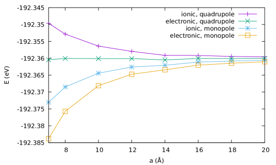
Figure 7: The energy of an Li⁺ ion in a cubic box as a function of cube size. Two different schemes for calculating the non-Coulombic energy are used, using the total ionic, and the total electronic, charge. Two different corrections for the charged system are used: the monopole term of the Makov–Payne correction, and both the monopole and quadrupole terms of that correction. The best convergence with size is seen with the full Makov–Payne correction, and the use of the ionic charge in the non-Coulombic energy.

Secondly pseudopotential codes will have a term in their total energy which arises from the non-Coulombic part of the $g=0$ components of the pseudopotentials used. This gives rise to no fields, but to an energy of

$$U=\frac{q}{V}\sum_{\textrm{ions}}V_{nc}$$ (16)

Where $q$ is the total charge, $V$ the cell volume, and $V_{nc}$ the non-Coulomb $g=0$ term of each ion’s pseudopotential. This expression is unambiguous in a neutral system, but in a charged system it matters whether $q$ is the total electronic charge or the total ionic charge (which can also be considered as the total charge from the electrons and the jellium). For the corrections in this paper, as for those in the original Makov and Payne paper[1], the total electronic charge must be used. Historically this is the value used by Castep[29], but recent versions of Castep use the total ionic charge, as does Abinit[30]. The use of the wrong value of $q$ here introduces an error in the energy which decays as $1/c$ in this 2D geometry.

This point is illustrated by a calculation on a 0D system of a single Li⁺ ion in a cubic box of varying sizes. A 900eV basis set cut-off was used. Figure 7 shows the energies after applying the Makov–Payne correction using both the ionic and electronic total charge in equation 16. It can be seen that, if one merely includes the monopole term from the Makov–Payne correction, then using the ionic charge in equation 16 gives the better result. However, on using both the monopole and quadrupole corrections, the use of the electronic charge in equation 16 is seen to be much superior.

One can further strengthen this argument by considering a system of Li³⁺. Then only term in the energy will be the Ewald energy of the ions, as all terms involving electrons must be zero. The variation of the Ewald energy with cell size is exactly corrected by the Makov–Payne formula, so there should be no other size-dependent term in the energy. In other words, when there are no electrons, equation 16 should be independent of cell size, and so the value of $q$ must be the electronic charge.

7 Conclusions

A self-consistent correction for modelling charged surfaces has been presented. Unlike the post hoc corrections, it produces rapid convergence with vacuum size of the energy and of other properties dependent on the wavefunctions or ground state charge density, such as the quadrupole moment. The energy convergence is exponential in the width of the vacuum region, and depends on the longest periodic distance parallel to the surface. In contrast the post hoc corrections do not produce exponential convergence, and their convergence rate depends on the thickness of the slab modelled. Though a vacuum region must be present, in order to contain the discontinuity in the potential, it is not subject to the constraint of being wider than the slab’s thickness, as methods such as truncated Coulomb potentials require.

The corrections presented are easy to add to existing density functional theory codes.

8 Acknowledgements

The author thanks Dr John Biggins and Prof. Volker Heine for helpful discussions. This work was supported by EPSRC grant number EP/P034616/1.

References

References

- [1] Makov G and Payne M C 1995 Phys. Rev. B 52 4014
- [2] Khazaei M, Ranjbar A, Esfarjani K, Bogdanovski D, Dronskowski R and Yunoki S 2018 Phys. Chem. Chem. Phys. 20(13) 8579
- [3] Wu S S, Huang T X, Lin K Q, Yao X, Hu J T, Tang D L, Bao Y F and Ren B 2019 2D Materials 6 045052
- [4] Li X, Guo T, Zhu L, Ling C, Xue Q and Xing W 2018 Chemical Engineering Journal 338 92
- [5] Bal K M and Neyts E C 2018 Phys. Chem. Chem. Phys. 20 8456
- [6] Patil U and Caffrey N M 2019 Phys. Rev. B 100 075424
- [7] Yeh I C and Berkowitz M L 1999 J. Chem. Phys. 111 3155
- [8] Jarvis M R, White I D, Godby R W and Payne M 1997 Phys. Rev. B 56 14972
- [9] Hine N D M, Dziedzic J, Haynes P D and Skylaris C K 2011 The Journal of Chemical Physics 135 204103
- [10] Komsa H P, Berseneva N, Krasheninnikov A V and Nieminen R M 2014 Phys. Rev. X 4 031044
- [11] Nattino F, Dupont C, Marzari N and Andreussi O 2019 J. Chem. Th. and Comput. 15 6313
- [12] Martyna G J and Tuckerman M E 1999 J. Chem. Phys. 110 2810–2821
- [13] Otani M and Sugino O 2006 Phys. Rev. B 73 115407
- [14] Dabo I, Kozinsky B, Singh-Miller N E and Marzari N 2008 Phys. Rev. B 77 115139
- [15] Dabo I, Kozinsky B, Singh-Miller N E and Marzari N 2011 Phys. Rev. B 84 159910(E)
- [16] Rozzi C A, Varsano D, Marini A, Gross E K U and Rubio A 2006 Phys. Rev. B 73(20) 205119
- [17] Krukowski S, Kempisty P and Strak P 2013 J. Appl. Phys 114 143705
- [18] Komsa H P and Pasquarello A 2013 Phys. Rev. Lett. 110(9) 095505
- [19] Freysoldt C and Neugebauer J 2018 Phys. Rev. B 97(20) 205425
- [20] Fraser L M, Foulkes W M C, Rajagopal G, Needs R J, Kenny S D and Williamson A J 1996 Phys. Rev. B 53 1814
- [21] Leslie M and Gillan N J 1985 J. Phys. C: Solid State Physics 18 973
- [22] Ballenegger V, Arnold A and Cerda J J 2009 J. Chem. Phys. 131 094107
- [23] Lozovoi A and Alavi A 2003 Phys. Rev. B 68 245416
- [24] Neugebauer J and Scheffler M 1992 Phys. Rev. B 46 16067
- [25] Francis G P and Payne M C 1990 J. Phys.: Cond. Matt. 2 4395
- [26] Clark S J, Segall M D, Pickard C J, Hasnip P J, Probert M J, Refson K and Payne M 2005 Z. Kristall. 220 567–570
- [27] Rutter M J 2018 Computer Physics Communications 225 174
- [28] Rutter M J and Heine V 1997 J. Phys.: Cond. Matt. 9 8213
- [29] Payne M C, Teter M P, Allan D C, Arias T A and Joannopoulos J D 1992 Rev. Mod. Phys. 64 1045
- [30] Gonze X, Jollet F, Abreu Araujo F, Adams D, Amadon B, Applencourt T, Audouze C, Beuken J M, Bieder J, Bokhanchuk A, Bousquet E, Bruneval F, Caliste D, Côté M, Dahm F, Da Pieve F, Delaveau M, Di Gennaro M, Dorado B, Espejo C, Geneste G, Genovese L, Gerossier A, Giantomassi M, Gillet Y, Hamann D, He L, Jomard G, Laflamme Janssen J, Le Roux S, Levitt A, Lherbier A, Liu F, Lukacevic I, Martin A, Martins C, Oliveira M, Poncé S, Pouillon Y, Rangel T, Rignanese G M, Romero A, Rousseau B, Rubel O, Shukri A, Stankovski M, Torrent M, Van Setten M, Van Troeye B, Verstraete M, Waroquiers D, Wiktor J, Xu B, Zhou A and Zwanziger J 2016 Computer Physics Communications 205 106 – 131 ISSN 0010-4655