AudioViewer: Learning to Visualize Sounds

Abstract

A long-standing goal in the field of sensory substitution is enabling sound perception for deaf and hard of hearing (DHH) people by visualizing audio content. Different from existing models that translate to hand sign language, between speech and text, or text and images, we target immediate and low-level audio to video translation that applies to generic environment sounds as well as human speech. Since such a substitution is artificial, without labels for supervised learning, our core contribution is to build a mapping from audio to video that learns from unpaired examples via high-level constraints. For speech, we additionally disentangle content from style, such as gender and dialect. Qualitative and quantitative results, including a human study, demonstrate that our unpaired translation approach maintains important audio features in the generated video and that videos of faces and numbers are well suited for visualizing high-dimensional audio features that can be parsed by humans to match and distinguish between sounds and words. Code and models are available at https://chunjinsong.github.io/audioviewer

1 Introduction

Humans perceive their environment through diverse channels, including vision and hearing. Because impairment in any sense can lead to drastic consequences, various approaches have been proposed to substitute lost senses, going all the way to recently popularized attempts to directly interface with neurons in the brain (e.g., NeuraLink [47]). One of the least intrusive approaches is to substitute audio with video, which is, however, challenging due to their high throughput and different modality.

In this paper, we propose a method to visualize audio with natural images in real-time, forming a live video that characterizes the audio content. It is a digital sign language with its own throughput, abstraction, automation, and readability trade-offs. Fig. 1 gives an overview of how short audio segments are sequentially mapped to frames of a live video of transforming figures.

Multiple approaches for audio-to-video translation exist, each striking a different compromise tailored for their application scenario. Lip-syncing the facial expressions of a virtual avatar from spoken audio [14, 57, 70, 6, 46, 78] allows deaf and hard of hearing (DHH) people to lip-read spoken texts. However, natural lip motion is a result of speaking and only contains a fraction of the audio content, which we validate in a comparative human study. Speech can also be translated to words with a recognition system [49]. For example, the spoken ’dog’ would be translated to the text ’dog’. This is intuitive, but such a translation is still indirect and does not contain any vocal feedback or style differences between male and female speakers [60, 76, 50]. Moreover, environmental sounds that cannot be indicated by a single word or lip motion, such as the echo of a dropped object or the repeating beep of an alarm, are ill-represented by all of these existing techniques. Traditional visual tools for deaf speech learning rely on spectrogram representations [16, 72, 71, 40], which are general but create unnatural images that humans rarely perceive in their surroundings and consequently have difficulties to comprehend.

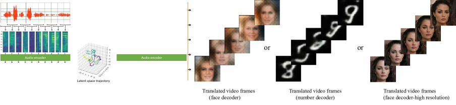
Figure 1: AudioViewer: A tool developed towards the long-term goal of helping hearing impaired persons to see what they can not hear. We map an audio stream to video and thereby use faces or numbers for visualizing the high-dimensional audio features intuitively. Different from the principle of lip reading, this can encode general sound and pass on information on the style of spoken language.

To overcome these limitations, we design AudioViewer as a low-level mapping—at the level of sounds and phones instead of words—which makes it immediate and could be used by infants before they have an understanding of words and language in general. It is similar to visualizing sounds with spectrograms but includes a machine learning component that disentangles factors and makes visualizations easier to comprehend by creating a series of natural images. The difficulty of creating such translation is that there is no canonical association to create paired labels between audio and video, which is necessary for supervised learning.

The underlying idea is to find high-level constraints that can be implemented as loss functions for machine learning and align the representation with human perception. We start from existing unpaired image translation techniques and equip them with additional properties. Our core contributions to realize perception-driven translation is the design, implementation, and evaluation of the following principles:

• To maintain the frequency of features, i.e., to map unusual sounds to unusual images, we utilize unsupervised learning and exploit cycle consistency to learn a joint structure between audio and video modalities.

• Humans are good at recognizing patterns that they see in their environment, particularly faces [1, 33, 64, 7, 29]. So we analyze mapping to natural image, including faces and hand-written digits of varying resolution.

• To separate styles, such as gender and dialect, from the content of individual phones and sounds, we disentangle the content by utilizing weak annotations of speech datasets.

• Humans are able to perceive complex spatial structures but quick and non-natural (e.g., flickering) changes lead to disruption and tiredness [59]. Hence, we enforce smoothness constraints on the learned mapping.

We demonstrate the feasibility of this AudioViewer approach with a working prototype and quantify the improvement brought about by our contributions by

• developing a low-level mapping from general sound to vision to help DHH people perceive the sound;

• introducing a new metric on the throughput, a lower bound for the loss of information content;

• a human study showing that words and phones can be better distinguished from the generated video features;

• a second human study which shows that a set of words in our novel representation can be learned with a success rate of 87% in as few as 16 attempts.

Clear improvements are gained over synthesized lip motions and plain spectrograms because a partial mapping loses important audio features and because content and style remain entangled in these baselines.

2 Related Work

In the following section, we first review the literature on audio and video generation, with a particular focus on cross-modal models. We then put our approach in context with existing assistive systems.

Classical audio to video translation. There is a large body of literature on audio-visual learning. We refer interested readers to recent survey [79] for a more comprehensive overview. Audio to video translation methods have mostly been designed as audio to scenes  [69, 56, 8, 21], audio to motions [65, 34, 61, 5, 58] and audio to talking faces [14, 57, 70, 39, 30, 54, 77, 6, 78, 46]. However, the translated scene images and body motions generated from sounds are at a high abstraction level, such as mapping the word dog to the image of a dog, but do not contain any vocal feedback, preventing people from learning the sounds from the generated images directly. The most related works are those aiming for digital dubbing or lip-syncing facial expressions to spoken audio [14, 57, 70, 39, 30, 54, 77, 6, 78, 46]. In contrast to our setting, these tasks are typically learned from paired examples, videos with audio lines, e.g., a talking person where the correspondence of lip motion, expressions and facial appearance to the spoken language is used to train the relation between sound and mouth opening. However, there are multiple sounds that correlate with the same lip and facial motion and others that do not correlate at all. By contrast, our unpaired translation mechanism is designed to map the entire audio spectrum.

Audio and video generation models. Image generation models predominantly rely on GAN [20] and VAE [38, 24] formulations. The highest image fidelity is attained with hierarchical models that inject noise and latent codes at various network stages by changing their feature statistics [27, 36]. For audio, only a few methods operate on the raw waveform [32]. It is more common to use spectrograms and to apply convolutional models inspired by the ones used for image generation [25, 13, 2]. We use cross-modal VAEs as a basis to learn the important audio and image features in terms of their frequency.

Cross-modal latent variable models. CycleGAN and its variations [80, 62] have considerable success in performing cross-modal unsupervised domain transfer, for medical imaging [23, 67] and audio to visual translation [21], but often encode information as a high-frequency signal that is invisible to the human eye and susceptible to adversarial attacks [9]. An alternative approach involves training a VAE, subject to a cycle-consistency condition  [31, 73], but these works were restricted to domain transfers within a single modality. Most similar is the joint audio and video model proposed by Tian et al. [66], which uses a VAE to map between two incompatible latent spaces using supervised alignment of attributes. However, it operates on a word, not phoneme level, and has no mechanism to ensure temporal smoothness nor information throughput. Our contributions address these shortcomings. Relatedly, encoder-decoder and GAN models have been applied to generating video reconstructions of lip movements based on audio data [10, 4, 68, 77, 78, 46], however, due to mapping ambiguities between phonemes and visemes, lip movements are not a reliable source of feedback for learning sound production [43, 48, 3, 17], which we further confirm with our evaluation.

Deaf speech support tools. Improvements in speech production for DHH people have been achieved through non-auditory aids and these improvements persist beyond learning sessions and extend to words not encountered during the sessions [60, 76, 50]. While electrophysiological [22, 37] and haptic learning aids [15] have demonstrated efficacy for improving speech production, such techniques can be more invasive, especially for young children, as compared to visual aids. Elssmann et al. [16] demonstrate visual feedback from the Speech Spectrographic Display (SSD) [60] is equally effective at improving speech production as compared with feedback from a speech-language pathologist. Alternative graphical plots generated from transformed spectral data have been explored by [72, 71, 40], which aim at improving upon spectrograms by creating plots that are more distinguishable with respect to speech parameters. Other methods aim at providing feedback by explicitly estimating vocal tract shapes [51]. In addition, Levis et al. [42] demonstrate that distinguishing between discourse-level intonation (intonation in conversation) and sentence-level intonation (intonation of sentences spoken in isolation) is possible through speech visualization and argues that deaf speech learning could be further improved by incorporating the former. Commercially, products such as the IBM’s Speech Viewer [28] are available to the public. Our image generation approach extends these spectrogram visualization techniques by leveraging the generative ability of VAEs in creating a mapping to a more natural video representation, which we show leads to improved recognition.

Sensory substitution and audio visualization. Related to our work is the field of sensory substitution, whereby information from one modality is provided to an individual through a different modality. While many sensory substitution methods focus on substituting visual information into other senses like tactile or auditory stimulation to help visual rehabilitation [45, 26, 19], few methods target substituting the auditory modality with visualization. Music visualization approaches generate visualizations of songs such that users can browse songs more efficiently without listening to them [74, 63]. On the learning side, [75] visualize the intonation and volume of each word in speech by the font size enables learning narration strategies. Different from the introduced above, our model tries to visualize speech and other audio at the phoneme and sound level with deep learning models instead of selected hand-crafted features.

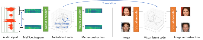
Figure 2: Overview. A joint latent encoding is learned with audio and video VAEs that are linked with a translation network and augmented with a smoothness constraint ($\Delta v$ annotation) and supplemented with disentangled training.

3 Method

Our goal is to translate a audio signal $\mathbf{A}=(\mathbf{a}_{1},\cdots,\mathbf{a}_{T_{A}})$ into a video visualization $\mathbf{V}=(\mathbf{I}_{1},\cdots,\mathbf{I}_{T_{V}})$, where $\mathbf{a}_{i}\in\mathbb{R}$ are sound wave samples recorded over $T_{A}$ time steps and $\mathbf{I}_{i}$ are images representing the same content over $T_{V}$ frames. Supervised training is not possible in the absence of paired labels. Instead, we start by learning individual audio and video models without correspondence. These are subsequently linked with an unpaired audio-to-video translation network that conserves high-level properties such as smoothness, regularity, and information loss using cycle-consistency and other unsupervised objectives motivated in the introduction. Fig. 2 shows the individual steps. The audio encoder $E_{A}(\mathbf{a}_{i})$ yields a audio latent code $\mathbf{z}_{i}\in\mathcal{Z_{A}}$ and the visual decoder $D_{V}(\mathbf{z}_{i})$ outputs a corresponding image $\mathbf{I}_{i}$. This produces a video representation of the audio when applied sequentially. Section 3.4 introduces the handling of mismatching latent spaces with a translation network.

Equalizing sound and video dimensionality. A first technical problem lies in the higher audio sampling frequency (16000 Hz), that prevents a one-to-one mapping to 25 Hz video. We follow common practice and represent the sound wave with a mel-scaled spectrogram, $\mathbf{M}=(\mathbf{m}_{1},\dots,\mathbf{m}_{T_{M}})$, $\mathbf{m}_{i}\in\mathbb{R}^{F}$, where $F=80$ is the number of filter banks. It is computed via the short-time Fourier transform with a 25 ms Hanning window with 10 ms shifts. In the following, we explain how to map from overlapping segments of length $T_{M}=20$ (covering $200$ ms) to corresponding video frames.

3.1 Audio Encoding

Given unlabelled audio and video sequences, we start by learning independent encoder-decoder pairs $(E_{A},D_{A})$ for sound and $(E_{V},D_{V})$ for video. We use probabilistic VAEs since these do not only learn a compact representation of the latent structure, but also allow us to control the shape of the latent distribution to be a standard normal distribution. Let $\mathbf{x}$ be a sample from the unlabelled audio set. We optimize over all samples using the VAE objective [38]:

$$\begin{split}{\mathcal{L}}(\mathbf{x})=-D_{\mathrm{KL}}(q_{\phi}(\mathbf{\mathbf{z}}|\mathbf{x})\|p_{\theta}(\mathbf{z}))\\ +\mathbb{E}_{q_{\phi}(\mathbf{\mathbf{z}}|\mathbf{x})}{\big{(}}\log p_{\theta}(\mathbf{x}|\mathbf{z}){\big{)}},\end{split}$$ (1)

with $D_{\mathrm{KL}}$, the Kullback-Leibler divergence, $q_{\phi}(\mathbf{z}|\mathbf{x})$ and $p_{\theta}(\mathbf{x}|\mathbf{z})$, the latent code and output domain posterior, respectively. These have a parametric form, with

$$q_{\phi}(\mathbf{z}|\mathbf{x}) ={\mathcal{N}}({\boldsymbol{\rho}}(\mathbf{x}),{\boldsymbol{\omega}}^{2}(\mathbf{x})\mathbf{I})\text{ and }$$ (2)

$$p_{\theta}(\mathbf{x}|\mathbf{z}) ={\mathcal{N}}({\boldsymbol{\mu}}(\mathbf{z}),{\boldsymbol{\sigma}}^{2}(\mathbf{z})\mathbf{I}),$$ (3)

where ${\boldsymbol{\rho}}$ and $\boldsymbol{\omega}$ are the output of the encoder and $\boldsymbol{\mu}$ and $\boldsymbol{\sigma}$ the output of the decoder. The dimention of $z$ is 256. We use the SpeechVAE model from Hsu et al. [25] that is widely used in sound generation.

3.2 Structuring the Audio Encoding

Content separation.

To better model speech, which we expect to have a higher information content compared to environment sounds, we further disentangle the style, such as gender and dialect, from the content conveyed in phones by leveraging datasets that have phone and speaker annotations. The separation follows that of established audio models [55]. Here we constrain the disentanglement by a recombined reconstruction loss term, $L_{rr}$. The details are provided in the supplemental file. Unless otherwise stated, we map only the audio content for visualization in our experiments.

Smoothness. We desire our latent space to change smoothly in time. However, the audio encoder has a small temporal receptive field, encoding time segments of 200ms. This lets encodings of subsequent sounds be encoded to distant latent codes leading to quick visual changes in the decoding. To counteract, we add a temporal smoothness loss on pairs of mel spectrogram segments $\{\mathbf{M}_{i,1},\mathbf{M}_{i,2}\}$ sampled at random time steps $\{t_{i,1},t_{i,2}\}$ spaced at most 800ms apart. We test two different pair-loss functions to enforce temporal smoothness in the embedded content vectors. First, by making changes in the latent space proportional to changes in time,

$$\mathcal{L}_{p,MSE}=\textstyle\frac{1}{N}\sum_{i}^{N}\left(\Delta\hat{\mathbf{z}}_{i}-\|t_{i,1}-t_{i,2}\|\right)^{2},$$ (4)

$\Delta\hat{\mathbf{z}}_{i}=s_{p}\cdot\|\mathbf{z}_{i,1}-\mathbf{z}_{i,2}\|$ the distance in the latent space obtained from $\{\mathbf{M}_{i,1},\mathbf{M}_{i,2}\}$, scale $s_{p}\in\mathbb{R}$ learned to find a scale between time and latent space dimensions. We found it advantageous to measure distances in the logarithmic scale,

$$\mathcal{L}_{p,\log}=\textstyle\frac{1}{N}\sum_{i}^{N}\left(\log{\Delta\hat{\mathbf{z}}_{i}}-\log{\|t_{i,1}-t_{i,2}\|}\right)^{2},$$ (5)

which lessens the weight for more distant encodings. Our final model uses $\mathcal{L}_{p,\log}$ We add this loss to the VAE objective with a weight of $\lambda_{p}=10^{3}$.

3.3 Image Autoencoder for Video Generation

We experiment with three different video models ranging from low-res to photo-realistic image generation: A linear PCA space, the image DFC-VAE model [24], and the image Soft-IntroVAE model [12]. We use pre-trained models, trained on collections of images. At first, naive unpaired translation is attained by encoding audio snippets sequentially and concatenating the audio encoder and video decoder of two VAEs with matching latent dimension and the same prior distribution $p(\mathbf{z})$ over $\mathbf{z}\in\mathcal{Z}_{V}$ to generate the frames of the output video.

3.4 Linking Audio and Visual Spaces

One of our key contributions is to meaningfully link the audio and video domain without paired examples. The naive concatenation explained in the previous section leads to low-quality results because smoothness in the latent space does not necessarily lead to smoothness in the output video, latent dimensions often do not match, and both encoders are only approximations to the true distribution.

When latent spaces have the same dimension, i.e., with [24] as visual model, we utilize a shared latent space and refine the weights of the video model to bridge structural differences. For [12], which has a larger latent space and is costly to train, we use a pre-trained model. To nevertheless link audio and video latent spaces, we introduce a translation network $T$ that maps the latent code $\mathbf{z}$ of the input audio segment to the visual latent variable $T(\mathbf{z})$. Fig. 3, visualizes this mapping and how the visual decoder $D_{V}$ subsequently decodes $T(\mathbf{z})$ to the output image $I$.

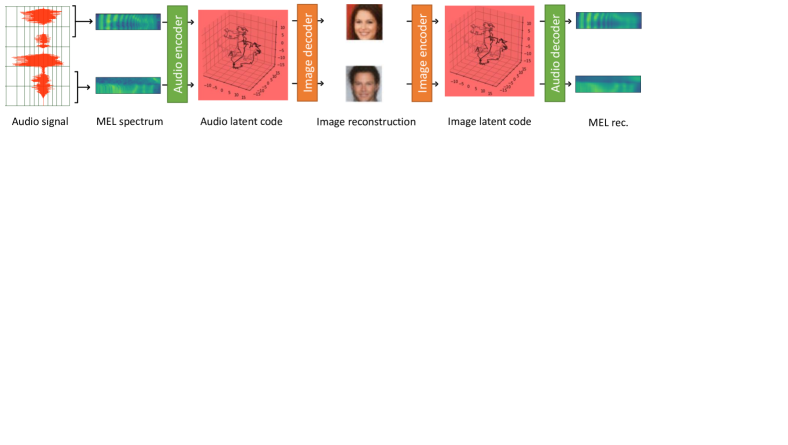
Figure 3: Cycle constraint. We apply a cycle constraint to ensures that the signal is preserved through video decoding and encoding.

Since our setting is unpaired we have to resort to self-supervised losses for modeling high-level constraints on auxiliary tasks instead of supervised learning. We explain them in the order of basic to more complex. First, to be a proper mapping, the range of $T(\mathbf{z})$ should be in the domain of the video decoder. Since the visual latent space fulfills the standard Gaussian distribution, we minimize its negative log-likelihood,

$$\mathcal{L}_{reg}=\lambda_{reg}\|T(\mathbf{z})\|^{2},$$ (6)

where $\lambda_{reg}=1.0$. Second, we minimize a lower bound on the information loss with the cycle consistency loss,

$$\mathcal{L}_{cycle}=\lambda_{cycle}\|E_{V}(D_{V}(T(\mathbf{z})))-T(\mathbf{z})\|,$$ (7)

that measures the difference between $T(\mathbf{z})$ and the reconstructed encoding of the generated image $I$ via visual encoder $E_{V}$ and is weighted by $\lambda_{cycle}=1.0$.

Meanwhile, consistent with Section 3.2, the changes in the generated image should be smooth. We ensure this with an additional temporal smoothness loss

$$\begin{split}\mathcal{L}_{\text{smooth}}=\lambda_{\text{smooth}}\frac{1}{N}\sum_{i}^{N}(\log(\left\|(I_{i,1}-I_{i,2})\right\|\\ s_{\text{smooth}})-\log\left\|t_{i,1}-t_{i,2}\right\|)^{2},\end{split}$$ (8)

which is applied on each pixel of the generated images. To further facilitate training of our multi-stage architecture, we also enforce a distance preserving loss on the latent spaces,

$$\begin{split}\mathcal{L}_{\text{iso}}=\lambda_{\text{iso}}\frac{1}{N}\sum_{i}^{N}(\log\left\|T(\mathbf{z}_{i,1})-T(\mathbf{z}_{i,2})\right\|\\ -\log(\left\|(\mathbf{z}_{i,1}-\mathbf{z}_{i,2})\right\|s_{\text{iso}}))^{2}.\end{split}$$ (9)

As in Section 3.2, we input the mel spectrogram segment pairs with random time steps $\{t_{i,1},t_{i,2}\}$, where $i$ represents the $i$th input pair. And $\lambda_{\text{iso}}=1.0$, $s_{\text{iso}}=5.0$, $\lambda_{\text{smooth}}=5.0$ and $s_{\text{smooth}}=0.001$. Both Eq. 8 and Eq. 9 help maintain the feature distances between latent spaces, preventing possible degenerate solutions for the translation network $T$ caused by Eq. 7 effectively. Note that neither of these self-supervised losses requires annotation. It therefore applies to environment sounds and could easily be finetuned for any language or dialect as long as an audio recording is available.

To measure the throughput of the entire system when using $T$ together with [12], we train a back-translation network $T^{\dagger}$ to reconstruct the input audio with

$$\mathcal{L}_{\text{back}}=\|D_{A}(T^{\dagger}(E_{V}(D_{V}(T(E_{A}(\mathbf{a}_{i}))))))-\mathbf{a}_{i}\|^{2}.$$ (10)

This reverse map training is a postprocess only used for evaluating throughput.

4 Experiments

We show qualitatively and quantitatively that AudioViewer conveys important audio features via visualizations of portraits or numbers, that it applies to speech and environment sounds, that it outperforms existing baselines, and that the task cannot be solved with mapping to lip motion [78]. The supplemental documents provides additional results, including example videos and human study details.

Quantitative metrics. We compare latent embeddings by the Euclidean distance, quantify differences in the mel spectrogram with the signal to noise ratio (SNR), and measure smoothness as the change in latent space position over time.

Perceptual studies. We perform two human studies to analyze the human capability to perceive the translated audio. As perceptual results may be subjective, we report statistics over 29 questions answered by 10-22 participants for each of the examined approaches for the distinguishability study and 9 participants for the learnability study. The details are given in the supplemental document.

Baselines. We compare to the most straight-forward speech to video translation, by i) mapping to lip and facial motion using the recent MakeItTalk method [78] and ii) comparing to spectogram visualizations as used in current assistive systems. To show that simpler approaches are insufficient, we experiment iii) with simpler variants of our approach and iv) principal component analysis (PCA) as further baselines. PCA yields a projection matrix $\mathbf{W}$ that rotates the training samples $\mathbf{u}_{i}$ by $\mathbf{z}_{i}=\mathbf{W}\mathbf{u}_{i}$ to have maximal variance. We use the reduced PCA version, where $\mathbf{W}$ maps to a $d$-dimensional space. A further important factor is the impact of the video domain, for which we compare digits vs. faces at the same resolution and low vs. high-resolution faces. In addition, we ablate the impact of our latent space priors and training strategies introduced in sections 3.2 and 3.4 as well as when disabling the style-content disentangling.

Datasets. We use the TIMIT dataset [18] for learning speech embeddings. It contains 5.4 hours of audio recordings (16 bit, 16 kHz) as well as time-aligned orthographic, phonetic and word transcriptions for 630 speakers of eight major dialects of American English, each reading ten phonetically rich sentences. We use the training split (462/50/24 non-overlapping speakers) of the KALDI toolkit [53]. The phonetic annotation is only used at audio encoder training time and as ground truth for the human study. In addition, we report how well a model trained on speech generalizes to environmental sounds on the ESC-50 dataset [52].

To test what kind of visualization is best for humans to perceive the translated audio, we train and test our model on three image datasets: The face attributes dataset CelebA-HQ [35](29000/1000 images for train/val respectively) and CelebA [44] (162770/19962 images for train/val respectively), the MNIST [41] datasets (60000/10000 images for train/val respectively). All shown results are with the high-res [12] decoder unless otherwise mentioned.

Runtime. The supplemental video contains a live demo. The AudioViewer using [24] is real-time capable, the inference time for a frame is 5 ms (low-res models) / 7.6 ms (high-res models) on an i7-9700KF CPU at 3.60GHz with a single NVIDIA GeForce RTX 2080 Ti.

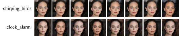
Figure 4: Environment sounds visualization. Although not trained for it, our approach also visualizes natural sounds. Here showing a clear difference between a chirping bird and an alarm clock.

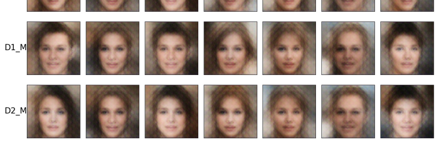
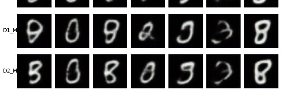
Figure 5: Phoneme similarity. The first phone of different words are distinctive (columns) while the speakers has a small influence (rows). This is consistent across image domains (Top to bottom: CelebA high-res, CelebA low-res, and MNIST).

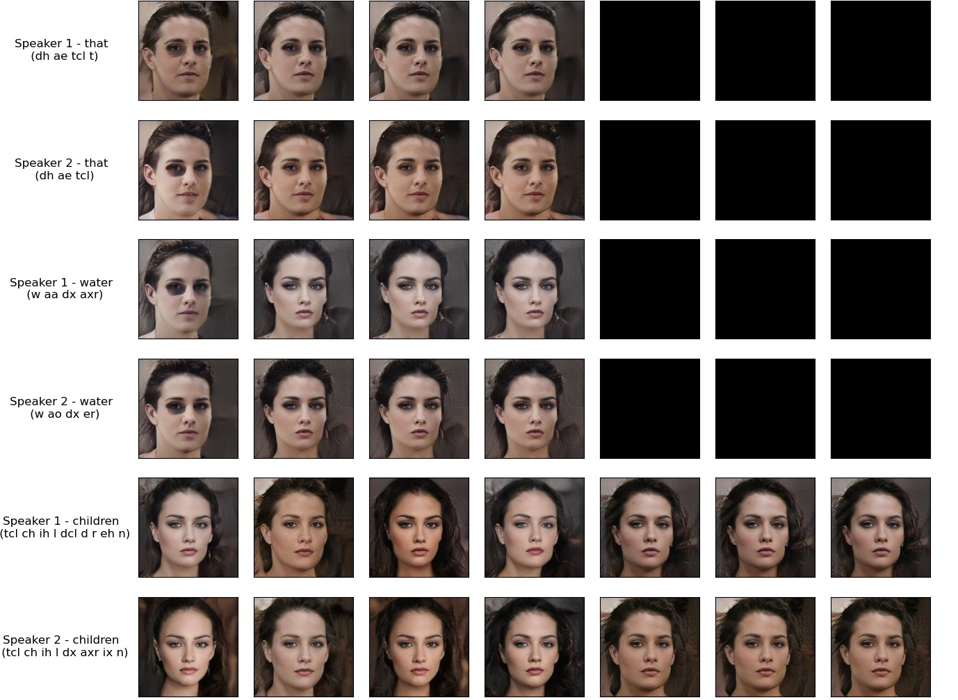
Figure 6: Word analysis. Instances (different rows) of the same words are encoded with a similar video sequence (single row) even though spoken by different speakers.

4.1 Visual Quality and Phonetics

A meaningful audio translation should encode similar sounds with similar visuals. Fig. 5 depicts such similarity and dissimilarity on the first 200 ms of a spoken word since these can be visualized with a single video frame. This figure compares the content encoding to MNIST and faces; both are well suited to distinguish sounds. The same word (column) has high visual similarity across different speakers (F#: female, M#: male; # the speaker ID) and dialects (D#) while words starting with different sounds are visually different. Multiple frames of entire words are shown in Fig. 6. Although trained entirely on speech, our sound-level formulation enables AudioViewer to also visualize environment sounds. Fig. 4 gives two examples on bird and alarm sounds. The supplemental contains additional ones.

We compare AudioViewer to the most related methods, including the lip synchronisation method [78] and mel spectogram visualizations as used in current assistive systems, as well as to simpler baselines. This first study test how well visualizations can be distinguished without requiring a time-intensive training period. This enables us to ask 29 questions to 60 participants and to cover 34 different words and phones, thereby showing generality.

4.2 Human Study I - Discriminating Sounds

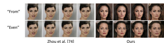
Figure 7: Comparison to lip-sync by [78]. While the lip synchronization looks very similar, the two words are clearly distinguishable in the AudioViewer visualizations.

Identifying and distinguishing sounds.

Our human study analyzes the ability to distinguish between visualizations of different sounds, similar to the ones show in Fig. 5 and the results are shown in Table 1. Overall, the users were able to correctly recognize visualizations for the same sound with an accuracy of 86.4% for the high-res CelebA content model and 85.0% vs. 79.7% for the low-res CelebA and MNIST content models, respectively. Broken down by tasks, users for the CelebA model achieve a better accuracy of 87.9% in correctly matching one of two visualizations against a reference (random guessing yields 50%), while for the task of grouping four visualizations into pairs, users achieved an accuracy of 85.7 % (random guessing yields 33.3%). The accuracy scores of MEL are far lower than those of our model, indicating that the patterns in mel spectrogram are more difficult to distinguish than the features generated by our learned model. In comparison to the lip synchronisation of Zhou et al. [78] AudioViewer enables a user to distinguish sounds significantly better. This is due to the almost identical lip motion for different phonemes (e.g. "d", "t" and "n") which makes them indistinguishable. Fig. 7 shows such a case of two words that look similar in lip motion but are clearly distinguishable in the AudioViewer visualizations.

Latent space disentanglement. Visualizing the style and content part separately with our full model significantly improves recognition scores. The disentangled face model increases the accuracy for distinguishing between speakers of a different sex from $43.3\pm 2.6\%$ to $78.0\pm 2.9\%$ and speakers of different dialects from $39.6\pm 7.2\%$ to $56.7\pm 5.7\%$, with $\pm$ reporting the standard error. In practice, AudioViewer should therefore use the full model and show separate visual decodings side by side or have the option to switch between content and style visualization. The entire study is reported in the supplemental document.

Table 1: User Study I results. User answer accuracy in percent ($\pm$ standard error) for distinguishing between visualizations of different sounds, broken down by question type and phone-pairs vs. words.

Dataset	MEL	Zhou [78]	MNIST	CelebA	CelebA
Resolution	(spectrum)	(high-res)	(low-res)	(low-res)	(high-res)
Matching	$65.5\pm 1.2$	$65.6\pm 3.6$	$77.4\pm 2.8$	$84.5\pm 3.7$	$\textbf{87.9}\pm\textbf{2.2}$
Grouping	$66.5\pm 2.1$	$39.5\pm 3.9$	$80.8\pm 2.2$	$85.2\pm 2.4$	$\textbf{85.7}\pm\textbf{1.8}$
Phones	$76.5\pm 1.9$	$69.5\pm 5.2$	$\textbf{91.8}\pm\textbf{2.5}$	$85.7\pm 3.0$	$87.0\pm 2.5$
Words	$60.0\pm 2.2$	$39.4\pm 2.9$	$73.8\pm 1.9$	$84.5\pm 2.3$	$\textbf{86.0}\pm\textbf{1.5}$
Overall	$66.2\pm 1.3$	$47.7\pm 2.7$	$79.7\pm 1.7$	$85.0\pm 1.8$	$\textbf{86.4}\pm\textbf{1.4}$

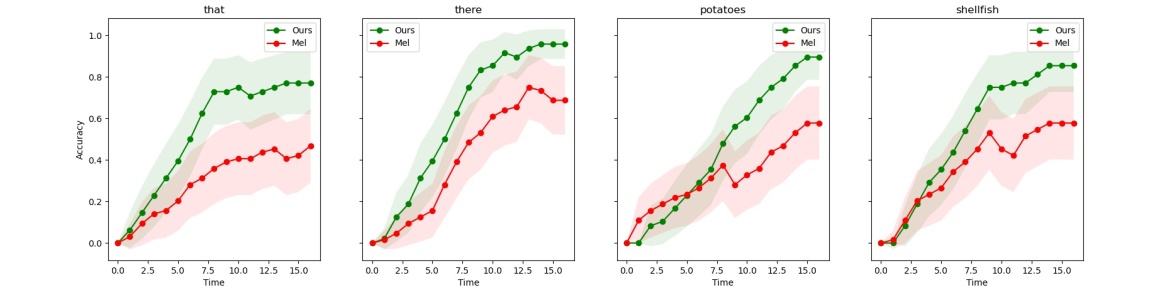
Figure 8: User Study II results. Subjects learn over time to distinguish words. The learning speed and accuracy of our model (green) outperform the baseline (red). Accuracy is plotted as the moving average of the success rate over trials.

4.3 Human Study II - Learning Sounds

In this second study we analyze learnability of our best model, determined in Study I and the ablation study, compared to using the best baseline, the mel spectogram (MEL). Four words were selected that include pairs that sound similar (that, there) and pairs that have the same length (potatoes, shellfish). They are spoken 4 times by different speakers with varying dialects and the same gender. During the study one word is visualized at a time. The participant is tasked to select the corresponding word. After each selection, the correct answer is given as feedback to enable learning.

Fig. 8 shows the average learning curves of nine participants that performed the same study for AudioViewer (green) and MEL (red). The curves reflect how the participants learn to recognize the same sound spoken by different people over time. The comparison shows that our method performs better than MEL in both learning speed and final accuracy for all of tested words (the shaded area is the standard error). The final accuracy after 16 rounds of learning is Ours 87.0% vs. MEL 57.8%, which reflects the learnability of our results. Additional details are included in the supplemental document.

4.4 Ablation Study

Information Throughput.

Audio models	Visual models	SNR(dB)
Audio PCA	Visual PCA	23.37
SpeechVAE [25]	DFC-VAE on CelebA	1.65
	DFC-VAE on MNIST	2.01
	DFC-VAE on CelebA (refined w/ $\mathcal{L}_{cycle}$)	4.43
	DFC-VAE on MNIST (refiend w/ $\mathcal{L}_{cycle}$)	0.78
SpeechVAE w/ $\mathcal{L}_{p,\log},$ $\mathcal{L}_{rr}$, dim=256	DFC-VAE on CelebA	0.84
	DFC-VAE on MNIST	0.81
	DFC-VAE on CelebA (refined w/ $\mathcal{L}_{cycle}$)	4.16
	DFC-VAE on MNIST (refiend w/ $\mathcal{L}_{cycle}$)	3.68
	Soft-Intro VAE on CelebA_HR (refined w/ $\mathcal{L}_{cycle}$)	2.01

Table 2: Throughput Analysis. The throughput estimated from audio to video shows that the cycle consistency improves greatly while additional constraints $\mathcal{L}_{p,\log}$, and $\mathcal{L}_{rr}$ incur only a small dip for improving smoothness. $dim$ indicates the dimension of the audio latent space. Results are consistent over different models.

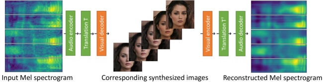
Figure 9: Throughput. A visualization of the lower bound on the information throughput when mapping from audio to video and back.

It is difficult to quantify the information throughput from audio to video as no ground truth is available in our setting. We propose to use the learned encoder and decoder to map from audio to video and back. The distance of the starting point to the reconstructed audio gives a lower bound on the loss of information, akin to CycleGAN. Fig. 9 gives an example and Table 2 summarizes relations quantitatively. The difference can also be analyzed qualitatively by listening and comparing the original and reconstructed audio samples, which are still recognizable for our full model. We found this throughput an important measure that correlated with performance in the human studies and enabled us to tune hyperparameters without performing an expensive study for each configuration. Note that the information throughput rivals other constraints such as smoothness. The goal is therefore to strike the best compromise. For instance, PCA attains the highest reconstruction accuracy but has poor smoothness (Table 3) and does not strike along the other dimensions. The disentangled space (lower half of Table 2) has a relatively low effect on the SNR, a reduction from $4.43$ to $4.16$, while providing improved interpretability. MNIST proved less stable to train and does not fair well with the cycle loss, perhaps due to a lower dimensionality that mismatches with the higher-dimensional audio encoding. The high-res CelebA model yields a lower SNR, likely because information is lost in the deeper network and the smoothness loss affects high-frequency details differently.

Temporal Smoothness Effectiveness. Mapping from audio to video with VAEs without constraints and PCA leads to choppy results. Table 3 shows that this corresponds to mean latent space velocities above 300 s^-1. It shows that the tested simpler solutions are insufficient. We visualize the gain in smoothness in Fig. 10 by plotting the high-dimensional latent trajectory embedded into three dimensions using multi-dimensional scaling (MDS) [11]. The gain is similar for all of the proposed variants. The supplemental videos show how the smoothness eases information perception.

Visual Domain Influence. Earlier work [7, 29] suggests that faces are suitable for representing high-dimensional data. Our experiments support this finding for the task at hand. Faces performed better than digits in our human study as facial models are richer in information. This is confirmed quantitatively by our throughput experiments, the SNR of the jointly trained CelebA models is larger than the MNIST models (visualized in Fig. 5). As expected, the human study also reveals that high-resolution faces work better than low-resolution faces.

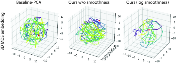
Figure 10: Smoothness evaluation by plotting the latent embedding of an audio snipped in 3D via dimensionality reduction. For PCA and w/o smoothness constraint, consecutive audio embeddings are scattered.

Audio models	SNR (dB)	Velocity ($\mathrm{s}^{-1}$)	Acc.($\mathrm{s}^{-2}$)
Audio PCA	23.37	329.02	13395.11
SpeechVAE[25]	21.89	280.09	11648.17
SpeechVAE w/ $\mathcal{L}_{p,\log}$	19.89	108.89	3052.19
SpeechVAE w/ $\mathcal{L}_{rr}$	7.73	80.80	2947.70
SpeechVAE w/ $\mathcal{L}_{rr}$,$\mathcal{L}_{p,\log}$	6.20	59.78	1530.81
SpeechVAE w/$\mathcal{L}_{rr}$, $\mathcal{L}_{p,\log}$, dim=256	6.28	65.63	1757.95

Table 3: We quantify the improvement in velocity and acceleration in relation to audio encode throughput in SNR on the best performing model, DFC-VAE on CelebA.

5 Limitations and Future Work

When presented with our visualizations the first time, users are unsure of what features they should focus on to distinguish. Our Study II shows that this improves with learning but similar sounds, such as that and there remain somewhat difficult to distinguish. Which is no surprise as the input audio is similar, but there is room to improve the expressiveness and make the visual language more intuitive. Moreover, the visualization of environment sounds lose higher frequency components since the audio models are trained on a speech dataset. To create a more natural mapping, we plan to map to lip motion for spoken sounds that are captured in the lip motion while maintaining the proposed general encoding for those that are not and for environment sounds.

6 Conclusion

We presented AudioViewer, a learning-based approach for visualizing audio, including speech and sounds, via generative models trained in the absence of paired examples. It can visualize sounds on faces and digits and outperforms all baselines in distinctiveness, including state-of-the-art lip synchronization and spectrograms as used in current assistive systems. Our face visualizations retain more information than lip motion and are easier to parse than spectrograms. Our proof of concept AudioViewer demo shows the feasibility of visualizing speech in real-time. We hope that our sensory substitution approach will catalyze the development of future tools for assisting people with auditorial handicaps.

7 Acknowledgement

We thank Ipek Oruk for her valuable comments and all participants of the user study for their time and contribution. This work was supported by the Compute Canada GPU servers.

References

- [1] Geoffrey K Aguirre, E Zarahn, and M D’esposito. An area within human ventral cortex sensitive to “building” stimuli: evidence and implications. Neuron, 21(2):373–383, 1998.
- [2] Jean-Pierre Briot, Gaëtan Hadjeres, and François-David Pachet. Deep learning techniques for music generation–a survey. arXiv preprint arXiv:1709.01620, 2017.
- [3] Luca Cappelletta and Naomi Harte. Phoneme-to-viseme mapping for visual speech recognition. In ICPRAM (2), pages 322–329, 2012.
- [4] Lele Chen, Zhiheng Li, Ross K Maddox, Zhiyao Duan, and Chenliang Xu. Lip movements generation at a glance. In Proceedings of the European Conference on Computer Vision (ECCV), pages 520–535, 2018.
- [5] Lele Chen, Sudhanshu Srivastava, Zhiyao Duan, and Chenliang Xu. Deep cross-modal audio-visual generation. In Proceedings of the on Thematic Workshops of ACM Multimedia 2017, Thematic Workshops ’17, page 349–357, New York, NY, USA, 2017. Association for Computing Machinery.
- [6] Lele Chen, Haitian Zheng, Ross Maddox, Zhiyao Duan, and Chenliang Xu. Sound to visual: Hierarchical cross-modal talking face generation. In Proceedings of the IEEE/CVF Conference on Computer Vision and Pattern Recognition (CVPR) Workshops, June 2019.
- [7] Herman Chernoff. The use of faces to represent points in k-dimensional space graphically. Journal of the American statistical Association, 68(342):361–368, 1973.
- [8] Jesper Haahr Christensen, Sascha Hornauer, and X Yu Stella. Batvision: Learning to see 3d spatial layout with two ears. In 2020 IEEE International Conference on Robotics and Automation (ICRA), pages 1581–1587. IEEE, 2020.
- [9] Casey Chu, Andrey Zhmoginov, and Mark Sandler. Cyclegan, a master of steganography. arXiv preprint arXiv:1712.02950, 2017.
- [10] Joon Son Chung, Amir Jamaludin, and Andrew Zisserman. You said that? arXiv preprint arXiv:1705.02966, 2017.
- [11] Michael AA Cox and Trevor F Cox. Multidimensional scaling. In Handbook of data visualization, pages 315–347. Springer, 2008.
- [12] Tal Daniel and Aviv Tamar. Soft-introvae: Analyzing and improving the introspective variational autoencoder. In Proceedings of the IEEE/CVF Conference on Computer Vision and Pattern Recognition, pages 4391–4400, 2021.
- [13] Hao-Wen Dong, Wen-Yi Hsiao, Li-Chia Yang, and Yi-Hsuan Yang. Musegan: Multi-track sequential generative adversarial networks for symbolic music generation and accompaniment. In Thirty-Second AAAI Conference on Artificial Intelligence, 2018.
- [14] Amanda Duarte, Francisco Roldan, Miquel Tubau, Janna Escur, Santiago Pascual, Amaia Salvador, Eva Mohedano, Kevin McGuinness, Jordi Torres, and Xavier Giro-i Nieto. Wav2pix: speech-conditioned face generation using generative adversarial networks. In IEEE International Conference on Acoustics, Speech and Signal Processing (ICASSP), volume 3, 2019.
- [15] Silvio P Eberhardt, Lynne E Bernstein, David C Coulter, and Laura A Hunckler. Omar a haptic display for speech perception by deaf and deaf-blind individuals. In Proceedings of IEEE Virtual Reality Annual International Symposium, pages 195–201. IEEE, 1993.
- [16] Sharon F Elssmann and Jean E Maki. Speech spectrographic display: use of visual feedback by hearing-impaired adults during independent articulation practice. American Annals of the Deaf, pages 276–279, 1987.
- [17] Adriana Fernandez-Lopez and Federico M Sukno. Optimizing phoneme-to-viseme mapping for continuous lip-reading in spanish. In International Joint Conference on Computer Vision, Imaging and Computer Graphics, pages 305–328. Springer, 2017.
- [18] John S Garofolo. Timit acoustic phonetic continuous speech corpus. Linguistic Data Consortium, 1993, 1993.
- [19] Louis H Goldish and Harry E Taylor. The optacon: A valuable device for blind persons. Journal of Visual Impairment & Blindness, 68(2):49–56, 1974.
- [20] Ian Goodfellow, Jean Pouget-Abadie, Mehdi Mirza, Bing Xu, David Warde-Farley, Sherjil Ozair, Aaron Courville, and Yoshua Bengio. Generative adversarial nets. In Advances in neural information processing systems, pages 2672–2680, 2014.
- [21] Wangli Hao, Zhaoxiang Zhang, and He Guan. Cmcgan: A uniform framework for cross-modal visual-audio mutual generation. In Thirty-Second AAAI Conference on Artificial Intelligence, 2018.
- [22] William J Hardcastle, Fiona E Gibbon, and Wilf Jones. Visual display of tongue-palate contact: electropalatography in the assessment and remediation of speech disorders. International Journal of Language & Communication Disorders, 26(1):41–74, 1991.
- [23] Yuta Hiasa, Yoshito Otake, Masaki Takao, Takumi Matsuoka, Kazuma Takashima, Aaron Carass, Jerry L Prince, Nobuhiko Sugano, and Yoshinobu Sato. Cross-modality image synthesis from unpaired data using cyclegan. In International workshop on simulation and synthesis in medical imaging, pages 31–41. Springer, 2018.
- [24] X. Hou, L. Shen, K. Sun, and G. Qiu. Deep feature consistent variational autoencoder. In 2017 IEEE Winter Conference on Applications of Computer Vision (WACV), pages 1133–1141, 2017.
- [25] Wei-Ning Hsu, Yu Zhang, and James Glass. Learning latent representations for speech generation and transformation. In Interspeech, pages 1273–1277, 2017.
- [26] Di Hu, Dong Wang, Xuelong Li, Feiping Nie, and Qi Wang. Listen to the image. In Proceedings of the IEEE/CVF Conference on Computer Vision and Pattern Recognition (CVPR), June 2019.
- [27] Xun Huang and Serge Belongie. Arbitrary style transfer in real-time with adaptive instance normalization. In Proceedings of the IEEE International Conference on Computer Vision, pages 1501–1510, 2017.
- [28] IBM. Speech viewer iii, 2004.
- [29] Robert JK Jacob and Howard E Egeth. The face as a data display. Human Factors, 18(2):189–200, 1976.
- [30] Amir Jamaludin, Joon Son Chung, and Andrew Zisserman. You said that?: Synthesising talking faces from audio. International Journal of Computer Vision, 127(11):1767–1779, 2019.
- [31] Ananya Harsh Jha, Saket Anand, Maneesh Singh, and VSR Veeravasarapu. Disentangling factors of variation with cycle-consistent variational auto-encoders. In European Conference on Computer Vision, pages 829–845. Springer, 2018.
- [32] Herman Kamper. Truly unsupervised acoustic word embeddings using weak top-down constraints in encoder-decoder models. In ICASSP 2019-2019 IEEE International Conference on Acoustics, Speech and Signal Processing (ICASSP), pages 6535–3539. IEEE, 2019.
- [33] Nancy Kanwisher, Damian Stanley, and Alison Harris. The fusiform face area is selective for faces not animals. Neuroreport, 10(1):183–187, 1999.
- [34] Tero Karras, Timo Aila, Samuli Laine, Antti Herva, and Jaakko Lehtinen. Audio-driven facial animation by joint end-to-end learning of pose and emotion. ACM Transactions on Graphics (TOG), 36(4):1–12, 2017.
- [35] Tero Karras, Timo Aila, Samuli Laine, and Jaakko Lehtinen. Progressive growing of gans for improved quality, stability, and variation. arXiv preprint arXiv:1710.10196, 2017.
- [36] Tero Karras, Samuli Laine, and Timo Aila. A style-based generator architecture for generative adversarial networks. In Proceedings of the IEEE Conference on Computer Vision and Pattern Recognition, pages 4401–4410, 2019.
- [37] William F Katz and Sonya Mehta. Visual feedback of tongue movement for novel speech sound learning. Frontiers in human neuroscience, 9:612, 2015.
- [38] Diederik P Kingma and Max Welling. Auto-encoding variational bayes. arXiv preprint arXiv:1312.6114, 2013.
- [39] Prajwal KR, Rudrabha Mukhopadhyay, Jerin Philip, Abhishek Jha, Vinay Namboodiri, and CV Jawahar. Towards automatic face-to-face translation. In Proceedings of the 27th ACM International Conference on Multimedia, pages 1428–1436, 2019.
- [40] Bernd J Kröger, Peter Birkholz, Rüdiger Hoffmann, and Helen Meng. Audiovisual tools for phonetic and articulatory visualization in computer-aided pronunciation training. In Development of multimodal interfaces: Active listening and synchrony, pages 337–345. Springer, 2010.
- [41] Yann LeCun, Léon Bottou, Yoshua Bengio, and Patrick Haffner. Gradient-based learning applied to document recognition. Proceedings of the IEEE, 86(11):2278–2324, 1998.
- [42] John Levis and Lucy Pickering. Teaching intonation in discourse using speech visualization technology. System, 32(4):505–524, 2004.
- [43] Björn Lidestam and Jonas Beskow. Visual phonemic ambiguity and speechreading. Journal of Speech, Language, and Hearing Research, 2006.
- [44] Ziwei Liu, Ping Luo, Xiaogang Wang, and Xiaoou Tang. Deep learning face attributes in the wild. In Proceedings of International Conference on Computer Vision (ICCV), December 2015.
- [45] Shachar Maidenbaum, Sami Abboud, and Amir Amedi. Sensory substitution: Closing the gap between basic research and widespread practical visual rehabilitation. Neuroscience & Biobehavioral Reviews, 41:3–15, 2014.
- [46] Rayhane Mama, Marc S. Tyndel, Hashiam Kadhim, Cole Clifford, and Ragavan Thurairatnam. Nwt: Towards natural audio-to-video generation with representation learning, 2021.
- [47] Elon Musk et al. An integrated brain-machine interface platform with thousands of channels. Journal of medical Internet research, 21(10):e16194, 2019.
- [48] Jacob L Newman, Barry-John Theobald, and Stephen J Cox. Limitations of visual speech recognition. In Auditory-Visual Speech Processing 2010, 2010.
- [49] Kuniaki Noda, Yuki Yamaguchi, Kazuhiro Nakadai, Hiroshi G Okuno, and Tetsuya Ogata. Audio-visual speech recognition using deep learning. Applied Intelligence, 42(4):722–737, 2015.
- [50] AM Öster. Teaching speech skills to deaf children by computer-based speech training. STL-Quarterly Progress and Status Report, 36(4):67–75, 1995.
- [51] Sang H Park, Dong J Kim, Jae H Lee, and Tae S Yoon. Integrated speech training system for hearing impaired. IEEE Transactions on Rehabilitation Engineering, 2(4):189–196, 1994.
- [52] Karol J Piczak. Esc: Dataset for environmental sound classification. In Proceedings of the 23rd ACM international conference on Multimedia, pages 1015–1018, 2015.
- [53] Daniel Povey, Arnab Ghoshal, Gilles Boulianne, Lukas Burget, Ondrej Glembek, Nagendra Goel, Mirko Hannemann, Petr Motlicek, Yanmin Qian, Petr Schwarz, et al. The kaldi speech recognition toolkit. In IEEE 2011 workshop on automatic speech recognition and understanding, number CONF. IEEE Signal Processing Society, 2011.
- [54] K R Prajwal, Rudrabha Mukhopadhyay, Vinay P. Namboodiri, and C.V. Jawahar. A lip sync expert is all you need for speech to lip generation in the wild. In Proceedings of the 28th ACM International Conference on Multimedia, MM ’20, page 484–492, New York, NY, USA, 2020. Association for Computing Machinery.
- [55] Kaizhi Qian, Yang Zhang, Shiyu Chang, Xuesong Yang, and Mark Hasegawa-Johnson. Autovc: Zero-shot voice style transfer with only autoencoder loss. In International Conference on Machine Learning, pages 5210–5219. PMLR, 2019.
- [56] Yue Qiu and Hirokatsu Kataoka. Image generation associated with music data. In Proceedings of the IEEE Conference on Computer Vision and Pattern Recognition Workshops, pages 2510–2513, 2018.
- [57] Najmeh Sadoughi and Carlos Busso. Speech-driven expressive talking lips with conditional sequential generative adversarial networks. IEEE Transactions on Affective Computing, 2019.
- [58] Eli Shlizerman, Lucio Dery, Hayden Schoen, and Ira Kemelmacher-Shlizerman. Audio to body dynamics. In Proceedings of the IEEE Conference on Computer Vision and Pattern Recognition, pages 7574–7583, 2018.
- [59] George Sperling. The information available in brief visual presentations. Psychological monographs: General and applied, 74(11):1, 1960.
- [60] Larkin W Stewart L and Houde R. A real-time sound spectrograph with implications for speech training for the deaf. In IEEE International Conference Accoustics Speech and Signal Processing, 1976.
- [61] Supasorn Suwajanakorn, Steven M Seitz, and Ira Kemelmacher-Shlizerman. Synthesizing obama: learning lip sync from audio. ACM Transactions on Graphics (TOG), 36(4):1–13, 2017.
- [62] Yaniv Taigman, Adam Polyak, and Lior Wolf. Unsupervised cross-domain image generation. arXiv preprint arXiv:1611.02200, 2016.
- [63] Takumi Takahashi, Satoru Fukayama, and Masataka Goto. Instrudive: A music visualization system based on automatically recognized instrumentation. In ISMIR, pages 561–568, 2018.
- [64] Michael J Tarr and Isabel Gauthier. Ffa: a flexible fusiform area for subordinate-level visual processing automatized by expertise. Nature neuroscience, 3(8):764–769, 2000.
- [65] Sarah Taylor, Taehwan Kim, Yisong Yue, Moshe Mahler, James Krahe, Anastasio Garcia Rodriguez, Jessica Hodgins, and Iain Matthews. A deep learning approach for generalized speech animation. ACM Transactions on Graphics (TOG), 36(4):1–11, 2017.
- [66] Yingtao Tian and Jesse Engel. Latent translation: Crossing modalities by bridging generative models. arXiv preprint arXiv:1902.08261, 2019.
- [67] Oleksandra Tmenova, Rémi Martin, and Luc Duong. Cyclegan for style transfer in x-ray angiography. International journal of computer assisted radiology and surgery, 14(10):1785–1794, 2019.
- [68] Konstantinos Vougioukas, Stavros Petridis, and Maja Pantic. End-to-end speech-driven facial animation with temporal gans. arXiv preprint arXiv:1805.09313, 2018.
- [69] Chia-Hung Wan, Shun-Po Chuang, and Hung-Yi Lee. Towards audio to scene image synthesis using generative adversarial network. In ICASSP 2019-2019 IEEE International Conference on Acoustics, Speech and Signal Processing (ICASSP), pages 496–500. IEEE, 2019.
- [70] Olivia Wiles, A Sophia Koepke, and Andrew Zisserman. X2face: A network for controlling face generation using images, audio, and pose codes. In Proceedings of the European Conference on Computer Vision (ECCV), pages 670–686, 2018.
- [71] Wang Xu, Xue Lifang, Yang Dan, and Han Zhiyan. Speech visualization based on robust self-organizing map (rsom) for the hearing impaired. In 2008 International Conference on BioMedical Engineering and Informatics, volume 2, pages 506–509. IEEE, 2008.
- [72] Dan Yang, Bin Xu, and Xu Wang. Speech visualization based on improved spectrum for deaf children. In 2010 Chinese Control and Decision Conference, pages 4377–4380. IEEE, 2010.
- [73] Dongsuk Yook, Seong-Gyun Leem, Keonnyeong Lee, and In-Chul Yoo. Many-to-many voice conversion using cycle-consistent variational autoencoder with multiple decoders. In Proc. Odyssey 2020 The Speaker and Language Recognition Workshop, pages 215–221, 2020.
- [74] Kazuyoshi Yoshii and Masataka Goto. Music thumbnailer: Visualizing musical pieces in thumbnail images based on acoustic features. In ISMIR, pages 211–216, 2008.
- [75] Linping Yuan, Yuanzhe Chen, Siwei Fu, Aoyu Wu, and Huamin Qu. Speechlens: A visual analytics approach for exploring speech strategies with textural and acoustic features. In 2019 IEEE International Conference on Big Data and Smart Computing (BigComp), pages 1–8. IEEE, 2019.
- [76] Cindy M Zaccagnini and Shirin D Antia. Effects of multisensory speech training and visual phonics on speech production of a hearing-impaired child. Journal of Childhool Communication Disorders, 15(2):3–8, 1993.
- [77] Hang Zhou, Yu Liu, Ziwei Liu, Ping Luo, and Xiaogang Wang. Talking face generation by adversarially disentangled audio-visual representation. In Proceedings of the AAAI Conference on Artificial Intelligence, volume 33, pages 9299–9306, 2019.
- [78] Yang Zhou, Xintong Han, Eli Shechtman, Jose Echevarria, Evangelos Kalogerakis, and Dingzeyu Li. Makelttalk: Speaker-aware talking-head animation. ACM Trans. Graph., 39(6), Nov. 2020.
- [79] Hao Zhu, Man-Di Luo, Rui Wang, Ai-Hua Zheng, and Ran He. Deep audio-visual learning: A survey. International Journal of Automation and Computing, 18(3):351–376, 2021.
- [80] Jun-Yan Zhu, Taesung Park, Phillip Isola, and Alexei A Efros. Unpaired image-to-image translation using cycle-consistent adversarial networks. In Proceedings of the IEEE international conference on computer vision, pages 2223–2232, 2017.