Nonparametric Regression in Nonstandard Spaces

Abstract

A nonparametric regression setting is considered with a real-valued covariate and responses from a metric space. One may approach this setting via Fréchet regression, where the value of the regression function at each point is estimated via a Fréchet mean calculated from an estimated objective function. A second approach is geodesic regression, which builds upon fitting geodesics to observations by a least squares method. These approaches are applied to transform two of the most important nonparametric regression estimators in statistics to the metric setting – the local linear regression estimator and the orthogonal series projection estimator. The resulting procedures consist of known estimators as well as new methods. We investigate their rates of convergence in a general setting and compare their performance in a simulation study on the sphere.

1 Introduction

Our goal is to estimate an unknown function $[0,1]\to\mathcal{Q},t\mapsto m_{t}$, which is not of a simple parametric form, where $(\mathcal{Q},d)$ is a general metric space. To this end, we have access to independent data $(x_{i},y_{i})_{i=1,\dots,n}$. We assume that the covariates are fixed as $x_{i}=\frac{i}{n}$, and $y_{i}$ is a random variable with values in $\mathcal{Q}$ such that its Fréchet mean is equal to $m_{x_{i}}$, i.e., $m_{x_{i}}=\operatorname*{arg\,min}_{q\in\mathcal{Q}}\mathbb{E}[d(y_{i},q)^{2}]$. We consider $\mathcal{Q}$ to be nonstandard, i.e., a metric space that is not isometric to a convex subset of a separable Hilbert space. Examples of nonstandard spaces are Riemannian manifolds, like the hypersphere $\mathbb{S}^{k}$, Hadamard spaces, like the space of phylogenetic trees [5], or Wasserstein spaces [1] in dimension greater than one.

The literature on statistical analysis in nonstandard spaces is vast. We refer the reader to [14] for an overview and only present a small glimpse here. The Fréchet mean [12] or barycenter $m\in\operatorname*{arg\,min}_{q\in\mathcal{Q}}\mathbb{E}[d(Y,q)^{2}]$ of a random variable $Y$ with values in the metric space $\mathcal{Q}$ lies at the heart of most analysis in nonstandard spaces. It can be viewed as a generalization of the Euclidean mean as $\mathbb{E}[X]=\operatorname*{arg\,min}_{q\in\mathbb{R}^{k}}\mathbb{E}[\left\nonscript\;|\nonscript\;X-q\right\nonscript\;|\nonscript\;^{2}]$ for a $\mathbb{R}^{k}$-valued random variable $X$ with $\mathbb{E}[\left\nonscript\;|\nonscript\;X\right\nonscript\;|\nonscript\;^{2}]<\infty$. In Alexandrov spaces, the sample Fréchet mean is shown to attain the parametric rate of convergence under certain conditions [13]. In Hadamard spaces, the theory of Fréchet means [25] and algorithms for their calculation [3] are well described. The Fréchet mean has been studied on Riemannian manifolds, e.g., [6]. In this setting, [9] (among others) show a central limit theorem. Nonparametric regression with metric target values is developed, e.g., in [8, 15, 19]. [17] present a regression technique with regularization by total variation. [23] discuss nonparametric regression techniques between Riemannian manifolds. Specifically in the Riemannian manifold of symmetric positive-definite matrices, [30] develop a version of a local polynomial regression estimators, where higher order polynomials in this space are defined using parallel transport. Based on the notion of geodesics, [11] introduces an analog of linear regression in symmetric Riemannian manifolds. These results are generalized and extended in [7].

1.1 Model

Let $(\mathcal{Q},d)$ be a metric space. For $t\in[0,1]$, let $Y_{t}$ be a $\mathcal{Q}$-valued random variable with finite second moment, i.e., $\mathbb{E}[d(Y_{t},q)^{2}]<\infty$ for all $t\in[0,1]$ and $q\in\mathcal{Q}$. Let the regression function $m\colon[0,1]\to\mathcal{Q}$ be a minimizer $m_{t}\in\operatorname*{arg\,min}_{q\in\mathcal{Q}}\mathbb{E}[d(Y_{t},q)^{2}]$. Later, we will define certain smoothness conditions on $t\mapsto m_{t}$ (and on the change of the distribution of $Y_{t}$) to restrict the class of possible functions. We will consider nonparametric estimators which have access to following data: Let $x_{i}:=\frac{i}{n}$ and let $(y_{i})_{i=1,\dots,n}$ be independent random variables with values in $\mathcal{Q}$ such that $y_{i}$ has the same distribution as $Y_{x_{i}}$.

This model will be considered for two classes of metric spaces $\mathcal{Q}$: bounded metric spaces and Hadamard space. If a metric space $(\mathcal{Q},d)$ fulfills $\sup_{q,p\in\mathcal{Q}}d(q,p)<\infty$, then it is called bounded. This requirement simplifies the assumptions that require integrals of distances to be finite. Hadamard spaces are geodesic metric spaces of nonpositive curvature. Formally, a metric space $(\mathcal{Q},d)$ is Hadamard if and only if it is complete, nonempty, and for all $q,p\in\mathcal{Q}$, there is $z\in\mathcal{Q}$ such that $d(y,z)^{2}\leq\frac{1}{2}d(y,q)^{2}+\frac{1}{2}d(y,p)^{2}-\frac{1}{4}d(q,p)^{2}$ for all $y\in\mathcal{Q}$. Hilbert spaces and complete simply-connected Riemannian manifolds of nonpositive sectional curvature are Hadamard, but also spaces without smooth structure like metric trees [25, Proposition 3.4] or the space of phylogenetic trees [5].

To show the applicability in practice, the results are applied to the hyperspheres $\mathbb{S}^{k}$ and simulations are executed on the sphere $\mathbb{S}^{2}$.

1.2 Two Approaches

To construct an estimator for $t\mapsto m_{t}$, one may try to adapt a known Euclidean estimator to the new scenario. Two prominent approaches to this task are Fréchet regression [19] and geodesic regression [11].

Fréchet Regression. The regression function $m_{t}$ is the Fréchet mean of $Y_{t}$, i.e., the minimizer of $\mathbb{E}[d(Y_{t},q)^{2}]$ over $q\in\mathcal{Q}$. In Fréchet regression, we estimate the function $t\mapsto\mathbb{E}[d(Y_{t},q)^{2}]$ for every fixed $q\in\mathcal{Q}$ by an Euclidean estimator $t\mapsto\hat{F}_{t}(q)$ using the data $(x_{i},z_{q,i})_{i=1,\dots,n}\subseteq[0,1]\times\mathbb{R}$ with $z_{q,i}:=d(y_{i},q)^{2}$. In this step, we may use one of the standard nonparametric regression estimators for certain classes of functions $[0,1]\to\mathbb{R}$. Then $\hat{F}_{t}(q)$ is minimized over $q\in\mathcal{Q}$ for a fixed $t$ to obtain the estimator $\hat{m}_{t}$.

Geodesic Regression. Assume our metric space $\mathcal{Q}$ is equipped with an exponential map $\mathsf{Exp}\colon\Theta\to\mathcal{Q}$, where $\Theta\subseteq\mathsf{T}\mathcal{Q}\subseteq\mathcal{Q}\times\mathbb{R}^{k}$ is a subset of the tangent bundle of $\mathcal{Q}$. A geodesic starting in point $p\in\mathcal{Q}$ and continuing in the direction $v\in\mathsf{T}_{p}\mathcal{Q}$ of the tangent space $\mathsf{T}_{p}\mathcal{Q}=\left\{u\in\mathbb{R}^{k}\colon(p,u)\in\mathsf{T}\mathcal{Q}\right\}$ of $\mathcal{Q}$ at $p$ can be described as a function $\mathbb{R}\to\mathcal{Q},\,x\mapsto\mathsf{Exp}(p,xv)$ with $(p,v)\in\mathsf{T}\mathcal{Q}$. In geodesic regression with covariates $x_{i}\in\mathbb{R}$, we minimize the empirical squared error

$$\sum_{i=1}^{n}d(y_{i},\mathsf{Exp}(p,x_{i}v))^{2}$$ (1)

over $(p,v)\in\Theta$ to find the best fitting geodesic. All forms of geodesic regression built on this criterion or a modification of it. For example, we can extend it to multivariate regression

$$\sum_{i=1}^{n}d\!\left(y_{i},\mathsf{Exp}\!\left(p,\sum_{j=1}^{J}x_{i,j}v_{j}\right)\right)^{2}\,,$$ (2)

where $x_{i}\in\mathbb{R}^{J}$ and $v_{1},\dots,v_{J}\in\mathsf{T}_{p}\mathcal{Q}$ or more general feature regression

$$\sum_{i=1}^{n}d\!\left(y_{i},\mathsf{Exp}\!\left(p,\sum_{j=1}^{J}\psi_{j}(x_{i})v_{j}\right)\right)^{2}\,,$$ (3)

where $x_{i}\in\mathcal{X}$ for an arbitrary space of covariates $\mathcal{X}$ and features $\psi_{j}\colon\mathcal{X}\to\mathbb{R}$. Furthermore, we may introduce weights $w_{i,t}$, e.g., $w_{i,t}=K((x_{i}-t)/h)$ for a kernel $K$ and a bandwidth $h>0$ to localize the procedure, and obtain (here for one-dimensional covariates)

$$(\hat{m}_{t},\hat{\dot{m}}_{t})=\operatorname*{arg\,min}_{(p,v)\in\Theta}\sum_{i=1}^{n}w_{i,t}d(y_{i},\mathsf{Exp}(p,x_{i}v))^{2}\,.$$ (4)

In this paper, we do not require the existence of an exponential map in the sense of Riemannian geometry. Instead, $\mathsf{Exp}\colon\Theta\to\mathcal{Q},\Theta\subseteq\mathcal{Q}\times\mathbb{R}^{k}$ is required to fulfill certain distance bounds as described in our results on geodesic regression.

1.3 Contribution

We compare the two approaches of geodesic (Geo) and Frechet (Fre) regression on two regression estimators, namely local linear regression (Loc) and the orthogonal series estimator (Ort). This makes four estimation procedures, which we refer to as LocGeo, LocFre, OrtGeo, and OrtFre. For the resulting estimators, which we denote as $\hat{m}_{t}$, our goal is to show explicit finite sample bounds of the mean integrated squared error (MISE) of the form $\int_{0}^{1}\mathbb{E}[d(m_{t},\hat{m}_{t})^{2}]\mathrm{d}t\leq Cn^{-\alpha}$ for constants $C,\alpha>0$. We are not interested in optimal universal constants, but the dependence on further parameters, like a moment bound, is to be explicit. For LocGeo, LocFre, and OrtFre we find $\int_{0}^{1}\mathbb{E}[d(m_{t},\hat{m}_{t})^{2}]\mathrm{d}t\leq Cn^{-\frac{2\beta}{2\beta+1}}$, where $\beta>0$ is a smoothness parameter. Regarding the smoothness condition, we consider different models for different estimators. In particular, $\beta$ has a somewhat different meaning for each estimator. Nonetheless, the results are comparable and the optimal nonparametric rate of convergence $n^{-\frac{2\beta}{2\beta+1}}$ is shown to hold in these three cases.

• LocFre (section 2): [19] introduce local constant (Nadaraya–Watson) and local linear Fréchet regression for general bounded metric spaces. For the local linear estimator, they show $d(\hat{m}_{t},m_{t})\in\mathbf{O}_{\mathbb{P}}(n^{-\frac{2}{5}})$ and a more general version of this result, see Corollary 1 in their article. We show, for a general local polynomial Fréchet estimator of order $\ell\in\mathbb{N}_{0}$, the point-wise error bound $\mathbb{E}\left[d(m_{t},\hat{m}_{t})^{2}\right]\leq Cn^{-\frac{2\beta}{2\beta+1}}$ for a constant $C>0$ and a smoothness parameter $\beta>0$, $\lfloor\beta\rfloor=\ell$, which implies the same rate for the MISE, Theorem 1, Theorem 2. Our results are slightly more general with conditions slightly less demanding. Furthermore, bounds in expectation for finite $n$ are stronger than in $\mathbf{O}_{\mathbb{P}}$ and are needed to make the error bound of this estimator comparable to the others. As [19], we demand a smoothness condition not directly on $t\mapsto m_{t}$, but on the change of the probability density of $Y_{t}$ in $t$.

• OrtFre (section 3): We apply the approach of Fréchet regression to the orthogonal series projection estimator and arrive at a new estimator, OrtFre. For the trigonometric series as instance of an orthogonal series, we show $\mathbb{E}[\int_{0}^{1}d(m_{t},\hat{m}_{t})^{2}\mathrm{d}t]\leq Cn^{-\frac{2\beta}{2\beta+1}}$ for a smoothness parameter $\beta\geq 1$ and a constant $C>0$, Theorem 3, Theorem 4. As for LocFre the smoothness condition is a requirement on the change of the density of $Y_{t}$ in $t$.

• LocGeo (section 4): We apply the approach of geodesic regression to the classical local linear estimator to obtain LocGeo. A local polynomial regression estimator of arbitrary order in the Riemannian manifold of symmetric positive definite matrices was already introduced in [30]. In contrast, the results here are restricted to a first order expansion, but they are applicable to a wide range of metric spaces. We show a point-wise error bound of $\mathbb{E}[d(m_{t},\hat{m}_{t})^{2}]\leq Cn^{-\frac{2\beta}{2\beta+1}}$ for all $t\in[0,1]$, a smoothness parameter $\beta\in(1,2]$, and a constant $C>0$, which implies the same bound on the mean integrated squared error, Theorem 5, Theorem 6. For this result, we assume a smoothness condition, which generalizes the Hölder condition that is common for local linear estimators. It demands that the true function $t\mapsto m_{t}$ can be locally approximated at $t$ by a geodesic up to an error of order $|x-t|^{\beta}$ for $x$ close to $t$.

In section 5, we discuss a construction of an OrtGeo estimator: We apply the geodesic regression approach to the orthogonal series projection estimator. We do not show optimal rates of convergence, and argue that this estimator may be sub-optimal as the properties that make it appealing in Euclidean spaces are lost in nonstandard spaces. Nonetheless, we include an estimator with the trigonometric series as the chosen orthogonal series in our simulation study.

Our goal is to make all theorems as general as reasonably possible. This manifests in quite abstract statements. To get a gist of the meaning of the abstract objects, we apply the general theorems on the hypersphere: 1, 2, and 3. These corollaries illustrate our results and show that they are indeed applicable to explicit and interesting nonstandard spaces. Furthermore, abstract assumptions of the general theorems are justified by showing that they are fulfilled on the hyperspheres.

The sphere is also the metric space used in our simulation study, section 7. To fulfill a variance inequality, which is an assumption for all our results, we introduce a new family of distributions on the sphere, the contracted uniform distributions. All estimators are implemented using the statistical programming language R [21]. The resulting package is freely available at https://github.com/ChristofSch/spheregr. Our experiments confirm and illustrate the theoretical findings.

The proofs of all results can be found in the appendix A. They partially built upon techniques developed in [22]. The major tools to prove results in this setting are empirical process theory with chaining, e.g. [29] or [26], and a technique called slicing or peeling, e.g., [28]. The proofs for local regression techniques partially follow the Euclidean version in [27, section 1.6], for trigonometric regression we build upon [27, section 1.7].

1.4 Notation and Conventions

Assumptions are named in small caps, e.g., Moment. The names of the presented methods are set in a typewriter font, e.g., LocFre.

We use a lower case $c$ for universal constants $c>0$. If the value depends on a variable, we indicate this by an index, e.g., $c_{\kappa}$ is a constant that depends only on $\kappa$. We do not specify the values of such constants. They are silently understood to take an appropriate value. Furthermore, the value may vary between two occurrences of such a constant.

A capital $C$ indicates a constant that has further meaning, which is usually described by a three letter index, e.g., we may require a moment condition $\mathbb{E}[d(Y_{t},m_{t})^{2}]\leq C_{\mathsf{Mom}}$ for all $t$ to be fulfilled. For simplicity, we assume these constants to be $\geq 1$, so that, e.g., $C_{\mathsf{Abc}}^{2}+C_{\mathsf{Abc}}C_{\mathsf{Xyz}}\leq cC_{\mathsf{Abc}}^{2}C_{\mathsf{Xyz}}$.

There is a silently underlying probability space $(\Omega,\Sigma_{\Omega},\mathbb{P})$. If a random variable, say $Y$, has values in a set, say $\mathcal{Y}$, that set is silently understood to be a measurable space $(\mathcal{Y},\Sigma_{\mathcal{Y}})$ and the random variable is a measurable map $Y\colon(\Omega,\Sigma_{\Omega})\to(\mathcal{Y},\Sigma_{\mathcal{Y}})$.

In each section, the estimator of the regression function at $t$ is denoted as $\hat{m}_{t}$. It depends on $n$ and potentially on further parameters like a bandwidth $h$, which will not be indicated in the notation but should be clear in the context.

For a vector $v\in\mathbb{R}^{k}$, we denote its Euclidean norm by $|v|$. For $\beta\in\mathbb{R}$, let $\lfloor\beta\rfloor$ be the largest integer strictly smaller than $\beta$. Let $(\mathcal{Q},d)$ be a metric space. To shorten the notation, we sometimes write $\overline{q,\!p}$ instead of $d(q,p)$ for $q,p\in\mathcal{Q}$. Define the ball $\operatorname{\mathrm{B}}(o,d,\delta):=\{q\in\mathcal{Q}\colon\overline{q,\!o}<\delta\}$ and the diameter $\operatorname{\mathsf{diam}}(\mathcal{Q},d):=\sup_{q,p\in\mathcal{Q}}\overline{q,\!p}$.

For the theorems below, we need a quantification of the entropy of the metric space $\mathcal{Q}$. To this end, we use Talagrands’s $\gamma_{2}$ [26] as defined below.

Definition 1.

1. Given a set $\mathcal{Q}$, an admissible sequence is an increasing sequence $(\mathcal{A}_{k})_{k\in\mathbb{N}_{0}}$ of partitions of $\mathcal{Q}$ such that $\mathcal{A}_{0}=\{\mathcal{Q}$} and the cardinality of $\mathcal{A}_{k}$ is bounded as $\#\mathcal{A}_{k}\leq 2^{2^{k}}$ for $k\geq 1$.

   By an increasing sequence of partitions we mean that every set of $\mathcal{A}_{k+1}$ is contained in a set of $\mathcal{A}_{k}$. We denote by $A_{k}(q)$ the unique element of $\mathcal{A}_{k}$ which contains $q\in\mathcal{Q}$.

2. Let $(\mathcal{Q},d)$ be a pseudo-metric space, i.e., $d$ is symmetric, fulfills the triangle inequality, and $d(q,q)=0$ for all $q\in\mathcal{Q}$. Define

   $$\gamma_{2}(\mathcal{Q},d):=\inf\sup_{q\in\mathcal{Q}}\sum_{k=0}^{\infty}2^{\frac{k}{2}}\operatorname{\mathsf{diam}}(A_{k}(q),d)\,,$$ (5)

   where the infimum is taken over all admissible sequences in $\mathcal{Q}$.

1.5 Common Assumptions

Following assumption are made for all results on rates of convergence of regression estimators in this article. They are conditions needed to bound the rate of convergence when estimating Fréchet means – even without considering covariates, see [22, Theorem 1].

Assumptions 1.

• VarIneq: There is $C_{\mathsf{Vlo}}\in[1,\infty)$ such that $C_{\mathsf{Vlo}}^{-1}\,\overline{q,\!m_{t}}^{2}\leq\mathbb{E}[d(Y_{t},q)^{2}-d(Y_{t},m_{t})^{2}]$ for all $q\in\mathcal{Q}$ and $t\in[0,1]$.

• Entropy: There are $C_{\mathsf{Ent}}\in[1,\infty)$ and $\alpha\in[1,2)$ such that

  $$\gamma_{2}(\mathcal{B},d)\leq C_{\mathsf{Ent}}\max(\operatorname{\mathsf{diam}}(\mathcal{B},d),\operatorname{\mathsf{diam}}(\mathcal{B},d)^{\alpha})$$ (6)

  for all $\mathcal{B}\subseteq\mathcal{Q}$.

• Moment: There are $\kappa>\frac{2}{2-\alpha}$ and $C_{\mathsf{Mom}}\in[1,\infty)$ such that $\mathbb{E}[d(Y_{t},m_{t})^{\kappa}]^{\frac{1}{\kappa}}\leq C_{\mathsf{Mom}}$ for all $t\in[0,1]$.

Remark 1.

• VarIneq: This condition is also called variance inequality and is well-known in the context of Fréchet means in Alexandrov spaces, [25, 18, 13]. VarIneq is a condition on the noise distribution and the geometry of the metric space. It can be viewed as a quantitative version of the condition of unique Fréchet means $m_{t}$ of $Y_{t}$. The variance inequality not only ensures uniqueness of $m_{t}$, it also requires the objective function $\mathbb{E}[\overline{Y_{t},\!q}^{2}]$ to grow quadratically in the distance of a test point $q$ to the minimizer $m_{t}$. Intuitively, this is fulfilled when the noise distribution is not too similar to a distribution that has nonunique Fréchet means.

  VarIneq is always true in Hadamard spaces [25, Proposition 4.4], which are geodesic metric spaces with nonpositive curvature and include the Euclidean spaces. For a variance inequality in spaces of nonnegative curvature, see [2, Theorem 3.3]. Furthermore, 1 below shows an explicit construction of distributions fulfilling VarIneq. We use this in section 7 to construct a distribution for our simulations on the sphere.

• Entropy: This condition can be viewed as a quantitative version of the requirement that balls in $\mathcal{Q}$ are totally bounded.

  We use Talagrand’s $\gamma_{2}$ to formulate the entropy condition. Let $\mathcal{B}\subseteq\mathcal{Q}$. It holds

  $$\gamma_{2}(\mathcal{B},d)\leq\int_{0}^{\infty}\sqrt{\log\!\left(N(\mathcal{B},d,r)\right)}\mathrm{d}r\,,$$ (7)

  where the integral is called entropy integral and

  $$N(\mathcal{B},d,r)=\min\mathopen{}\left\{k\in\mathbb{N}\,\bigg{|}\,\exists q_{1},\dots,q_{k}\in\mathcal{Q}\colon\mathcal{B}\subseteq\bigcup_{j=1}^{k}\operatorname{\mathrm{B}}(q_{j},d,r)\right\}\mathclose{}$$ (8)

  is the covering number. Thus, we can use bounds on the entropy integral to fulfill Entropy, which is more common in the statistics literature. In some circumstances $\gamma_{2}$ is strictly lower than the entropy integral [26, Exercise 4.3.11]. One can further weaken the entropy condition as done in [2] and [22], potentially at the cost of worse rates of convergence.

  In the Euclidean space $\mathbb{R}^{k}$, Entropy holds with $\alpha=1$ and $C_{\mathsf{Ent}}=2\sqrt{k}$. If $\operatorname{\mathsf{diam}}(\mathcal{Q},d)<\infty$, one can choose $\alpha=1$ without loss of generality as the ratio between $\operatorname{\mathsf{diam}}(\mathcal{B},d)$ and $\operatorname{\mathsf{diam}}(\mathcal{B},d)^{\alpha}$ is bounded by the constant $\operatorname{\mathsf{diam}}(\mathcal{Q},d)^{\alpha-1}$.

  Next we consider an example in which $\alpha>1$ is needed. Take countably infinitely many intervals of length 1 and glue them together such that they form an infinite binary tree. This space with its intrinsic distance $d$ is an example of a metric tree and a Hadamard space [25, Proposition 3.4]. A subset $\mathcal{B}$ in this space with diameter $2R$ has at most $3^{R+1}$ branches and all branches together have at most length $R3^{R+1}$. Thus, $N(\mathcal{B},d,r)\leq cR\exp(cR)/r$ and we can calculate the bound $\gamma_{2}(\mathcal{B},d)\leq c\max(R,R^{\frac{3}{2}})$.

• Moment: This condition can be described as a moment condition. In Euclidean spaces $\mathcal{Q}=\mathbb{R}^{k}$, $d=|\cdot|$, this is equivalent to $\mathbb{E}[\left\nonscript\;|\nonscript\;Y_{t}-\mathbb{E}[Y_{t}]\right\nonscript\;|\nonscript\;^{\kappa}]<C_{\mathsf{Mom}}^{\kappa}$. Note that, due to the triangle inequality, $\mathbb{E}[d(Y_{t},m_{t})^{\kappa}]<\infty$ if and only if $\mathbb{E}[d(Y_{t},q)^{\kappa}]<\infty$ for any $q\in\mathcal{Q}$ or, equivalently, for all $q\in\mathcal{Q}$.

Proposition 1 ([18, section 5]).

Let $(\mathcal{Q},d)$ be a proper Alexandrov space of nonnegative curvature. Let $Z_{1}$ be a random variable with values $\mathcal{Q}$ such that $\mathbb{E}[d(Z_{1},q)^{2}]<\infty$ for all $q\in\mathcal{Q}$. Let $m\in\operatorname*{arg\,min}_{q\in\mathcal{Q}}\mathbb{E}[\overline{Z_{1},\!q}^{2}]$ be any Fréchet mean of $Z_{1}$. For $a\in[0,1)$, let $Z_{a}:=\gamma_{m\to Z}(a)$, where, for $z\in\mathcal{Q}$, $\gamma_{m\to z}$ is a geodesic with $\gamma_{m\to z}(0)=m$, $\gamma_{m\to z}(1)=z$. Then

$$(1-a)\overline{q,\!m}^{2}\leq\mathbb{E}[\overline{Z_{a},\!q}^{2}-\overline{Z_{a},\!m}^{2}]$$ (9)

for all $a\in[0,1]$.

2 Local Fréchet Regression

We use the principles of Fréchet regression on local polynomial regression. This yields local polynomial Fréchet regression, LocFre, which was introduced (in the local constant and local linear forms) in [19].

Let $K\colon\mathbb{R}\to\mathbb{R}$ be a function, the kernel. For $\ell\in\mathbb{N}_{0}$, $h>0$, and $x,t\in[0,1]$ define

$$\Psi(x) :=\left(\frac{x^{k}}{k!}\right)_{k=0,\dots,\ell}\,,$$ (10)

$$B_{n,t} :=\frac{1}{nh}\sum_{i=1}^{n}\Psi\!\left(\frac{x_{i}-t}{h}\right)\Psi\!\left(\frac{x_{i}-t}{h}\right)\!^{\top}\!K\!\left(\frac{x_{i}-t}{h}\right)\,,$$ (11)

$$w_{i,t} :=\frac{1}{nh}\Psi(0)\!^{\top}\!B_{n,t}^{-1}\Psi\!\left(\frac{x_{i}-t}{h}\right)K\!\left(\frac{x_{i}-t}{h}\right)\,,$$ (12)

whenever $B_{n,t}$ is invertible. Note that $w_{i,t}$ depends on $n,(x_{j})_{j=1,\dots,n}$ and in particular on $h$, which is not indicated in the notation. A local polynomial Fréchet estimator of order $\ell$ is any element

$$\hat{m}_{t}\in\operatorname*{arg\,min}_{q\in\mathcal{Q}}\sum_{i=1}^{n}w_{i,t}d(y_{i},q)^{2}\,.$$ (13)

For denoting a smoothness condition required for this estimator to achieve the nonparametric rate of convergence, we need to refer to the Hölder class $\Sigma(\beta,L)$ for $\beta,L>0$. It is defined as the set of $\lfloor\beta\rfloor$-times continuously differentiable functions $f\colon[0,1]\to\mathbb{R}$ with $|f^{(\lfloor\beta\rfloor)}(t)-f^{(\lfloor\beta\rfloor)}(x)|\leq L\left|x-t\right|^{\beta-\lfloor\beta\rfloor}$ for all $x,t\in[0,1]$.

Assumptions 2.

• Kernel: There are $C_{\mathsf{Kmi}},C_{\mathsf{Kma}}\in[1,\infty)$ such that

  $$C_{\mathsf{Kmi}}^{-1}\mathds{1}_{[-\frac{1}{2},\frac{1}{2}]}(x)\leq K(x)\leq C_{\mathsf{Kma}}\mathds{1}_{[-1,1]}(x)$$ (14)

  for all $x\in\mathbb{R}$.

• HölderSmoothDensity: The function $[0,1]\to\mathcal{Q},\,t\mapsto m_{t}$ is continuous. Let $C_{\mathsf{Len}}\in[1,\infty)$ such that $\sup_{s,t\in[0,1]}d(m_{s},m_{t})\leq C_{\mathsf{Len}}$. Let $\mu$ be a probability measure on $\mathcal{Q}$. Let $C_{\mathsf{Int}}\in[1,\infty)$ such that $\int\overline{y,\!m_{0}}^{2}\mu(\mathrm{d}y)\leq C_{\mathsf{Int}}$. Let $y\to\rho(y|t)$ be the $\mu$-density of $Y_{t}$. Let $\beta>0$ with $\ell=\lfloor\beta\rfloor$. For $\mu$-almost all $y\in\mathcal{Q}$, there is $L(y)\geq 0$ such that $t\mapsto\rho(y|t)\in\Sigma(\beta,L(y))$. Furthermore, there is a constant $C_{\mathsf{SmD}}\in[1,\infty)$, $\int L(y)^{2}\mathrm{d}\mu(y)\leq C_{\mathsf{SmD}}^{2}$.

Kernel and a smoothness condition are classical requirements for a local polynomial estimators to obtain an optimal error bound [27, Proposition 1.13].

Remark 2.

• Kernel: This is a typical condition on kernels for local kernel regression, see also [27, Lemma 1.5]. It is fulfilled, e.g., by the rectangular kernel $\mathds{1}_{[-\frac{1}{2},\frac{1}{2}]}(x)$ or the Epanechnikov kernel $\frac{3}{4}(1-x^{2})\mathds{1}_{[-1,1]}(x)$. Kernel likely could be weakened to allow for a greater variety of kernels, e.g., higher order kernels.

• HölderSmoothDensity: If the noise distribution has a $\mu$-density and this density is smooth enough, HölderSmoothDensity can be interpreted as a smoothness condition on $t\mapsto m_{t}$: In a Euclidean space $\mathcal{Q}=\mathbb{R}^{k}$ with a location model $\rho(y|t)=f(|y-m_{t}|^{2})$ for a smooth function $f\colon[0,\infty)\to[0,\infty)$, we have $\partial_{t}\rho(y|t)=-2(y-m_{t})\!^{\top}\!\dot{m}_{t}f^{\prime}(|y-m_{t}|^{2})$, where $\dot{m}_{t}\in\mathbb{R}^{k}$ is the derivative of $x\mapsto m_{x}$ at $t$. If $f^{\prime}$ is smooth enough and bounded, the smoothness of $\partial_{t}\rho(y|t)$ is dominated by the smoothness of $m_{t}$. Informally, the density should be as least as smooth as the regression function, to view this condition as a typical smoothness assumption on the regression function. It is likely an artifact of the proof that we require the error density to be smooth.

Theorem 1 (LocFre Bounded).

Let $(\mathcal{Q},d)$ be a bounded metric space. Let $\beta>0$ with $\ell=\lfloor\beta\rfloor$. Let $\hat{m}_{t}$ be the local polynomial estimator of order $\ell$ with $h\geq\frac{c}{n}$ and $n\geq c$. Assume VarIneq, Entropy with $\alpha=1$, HölderSmoothDensity, Kernel. Then

$$\mathbb{E}\left[\overline{m_{t},\!\hat{m}_{t}}^{2}\right]\leq C_{1}h^{2\beta}+C_{2}(nh)^{-1}\,,$$ (15)

where

$$C_{1} =cC_{\mathsf{Vlo}}^{2}C_{\mathsf{Ker}}^{2}C_{\mathsf{SmD}}^{2}\operatorname{\mathsf{diam}}(\mathcal{Q},d)^{2}\,,$$

$$C_{2} =cC_{\mathsf{Vlo}}^{2}C_{\mathsf{Ent}}^{2}C_{\mathsf{Ker}}^{2}\operatorname{\mathsf{diam}}(\mathcal{Q},d)^{2}\,.$$

Theorem 2 (LocFre Hadamard).

Let $(\mathcal{Q},d)$ be a Hadamard space. Let $\beta>0$ with $\ell=\lfloor\beta\rfloor$. Let $\hat{m}_{t}$ be the local polynomial estimator of order $\ell$ with $c\geq h\geq\frac{c}{n}$ and $n\geq c$. Assume Moment, Entropy, HölderSmoothDensity, Kernel. Then, for all $t\in[0,1]$,

$$\mathbb{E}\left[\overline{m_{t},\!\hat{m}_{t}}^{2}\right]\leq C_{1}h^{2\beta}+C_{2}(nh)^{-1}\,,$$ (16)

where

$$C_{1} =c_{\alpha,\kappa}\left(C_{\mathsf{Kmi}}^{2}C_{\mathsf{Kma}}^{2}C_{\mathsf{SmD}}C_{\mathsf{Mom}}C_{\mathsf{Len}}C_{\mathsf{Int}}\right)^{\frac{2}{2-\alpha}}\,,$$

$$C_{2} =c_{\alpha,\kappa}\left(C_{\mathsf{Mom}}C_{\mathsf{Ent}}C_{\mathsf{Kmi}}^{2}C_{\mathsf{Kma}}^{2}\right)^{\frac{2}{2-\alpha}}\,.$$

The two theorems are derived from a more general result in the appendix, Theorem 7. We obtain the classical error bound for local polynomial estimators with a bias term $h^{2\beta}$ and a variance term $(nh)^{-1}$. If we set $h=n^{-\frac{1}{2\beta+1}}$, in both cases, we obtain the classical nonparametric rate of convergence $\mathbb{E}[\overline{m_{t},\!\hat{m}_{t}}^{2}]\leq Cn^{-\frac{2\beta}{2\beta+1}}$. By integrating the inequality, we obtain the same bound for the MISE $\mathbb{E}[\int_{0}^{1}\overline{m_{t},\!\hat{m}_{t}}^{2}\mathrm{d}t]$.

Remark 3.

Theorem 2 applied to the real line $(\mathcal{Q},d)=(\mathbb{R},|\cdot|)$ yields almost the same result as the standard result for Euclidean local polynomial regression [27, Proposition 1.13]. Aside from different constants, we require a finite moment of order $\kappa>2$ instead of $\kappa=2$ and the error density needs to change smoothly, see point HölderSmoothDensity in 2. It seems remarkable that the results are so close as we have to do without an inner product and without vector space structure in the space of responses.

3 Orthogonal Series Fréchet Regression

Let $(\psi_{j})_{j\in\mathbb{N}}$ be a sequence of functions that form an orthonormal base in $\mathbb{L}^{2}[0,1]$, in particular,

$$\int_{0}^{1}\psi_{j}(x)\psi_{\tilde{j}}(x)\mathrm{d}x=\delta_{j{\tilde{j}}}$$ (17)

for all $\tilde{j},j\in\mathbb{N}$, where $\delta_{j{\tilde{j}}}$ is the Kronecker delta. Let $N\in\mathbb{N}$. Define $\Psi_{N}:=(\psi_{j})_{j=1,\dots,N}$.

Assume the matrix $B_{n}:=\frac{1}{n}\sum_{i=1}^{n}\Psi_{N}(x_{i})\Psi_{N}(x_{i})\!^{\top}\!$ is invertible. The orthogonal series Fréchet regression estimator is

$$\hat{m}_{t}\in\operatorname*{arg\,min}_{q\in\mathcal{Q}}\Psi_{N}(t)\!^{\top}\!B_{n}^{-1}\frac{1}{n}\sum_{i=1}^{n}\Psi_{N}(x_{i})d(y_{i},q)^{2}\,.$$ (18)

For an explicit estimator, we have to choose an explicit orthogonal series. Because of its appealing theoretical properties among other things, the trigonometric series is a common choice. Let $(\psi_{j})_{j\in\mathbb{N}}$ be the trigonometric basis of $\mathbb{L}^{2}[0,1]$, i.e., for $x\in[0,1]$, $j\in\mathbb{N}$,

$$\psi_{1}(x) =1\,, \psi_{2j}(x) =\sqrt{2}\cos(2\pi jx)\,, \psi_{2j+1}(x) =\sqrt{2}\sin(2\pi jx)\,.$$ (19)

The trigonometric basis is orthonormal. Furthermore,

$$\frac{1}{n}\sum_{i=1}^{n}\psi_{j}(x_{i})\psi_{\tilde{j}}(x_{i})=\delta_{j{\tilde{j}}}$$ (20)

for $j,\tilde{j}\in\left\{1,\dots,n-1\right\}$, see [27, Lemma 1.7]. Thus, $B_{n}$ is the identity matrix if $N<n$ and the estimator simplifies to

$$\hat{m}_{t}\in\operatorname*{arg\,min}_{q\in\mathcal{Q}}\Psi_{N}(t)\!^{\top}\!\frac{1}{n}\sum_{i=1}^{n}\Psi_{N}(x_{i})d(y_{i},q)^{2}\,.$$ (21)

The appropriate smoothness class connected to the trigonometric basis $(\psi_{j})_{j\in\mathbb{N}}$ is the periodic Sobolev class $W^{\mathsf{per}}(\beta,L)$, see [27, Definition 1.11]. A function $f(x)=\sum_{j=1}^{\infty}\vartheta_{j}\psi_{j}(x)$ belongs to $W^{\mathsf{per}}(\beta,L)$ if and only if the sequence $\vartheta=(\vartheta_{j})_{j\in\mathbb{N}}$, $\vartheta_{j}=\int_{0}^{1}f(x)\psi_{j}(x)\mathrm{d}x$, of the Fourier coefficients of $f$ belongs to the ellipsoid $\mathcal{E}(\beta,L)$, which is defined as

$$\mathcal{E}(\beta,L)=\left\{\vartheta\in\ell^{2}(\mathbb{R})\colon\sum_{j=1}^{\infty}\vartheta_{j}^{2}a_{j}^{-2}\leq L^{2}\right\}\,,$$ (22)

where $a_{2j+1}=a_{2j}=(2j)^{-\beta}$, see [27, Proposition 1.14].

Assumptions 3.

• SobolevSmoothDensity: The function $[0,1]\to\mathcal{Q},\,t\mapsto m_{t}$ is continuous. Let $C_{\mathsf{Len}}\in[1,\infty)$ such that $\sup_{s,t\in[0,1]}d(m_{s},m_{t})\leq C_{\mathsf{Len}}$. Let $\mu$ be a probability measure on $\mathcal{Q}$. Let $C_{\mathsf{Int}}\in[1,\infty)$ such that $\int\overline{y,\!m_{0}}^{2}\mu(\mathrm{d}y)\leq C_{\mathsf{Int}}$. For all $t\in[0,1]$, the random variable $Y_{t}$ has a density $y\mapsto\rho(y|t)$ with respect to $\mu$. Let $\beta\geq 1$. For $\mu$-almost all $y\in\mathcal{Y}$, there is $L(y)\geq 0$ such that $t\mapsto\rho(y|t)\in W^{\mathsf{per}}(\beta,L(y))$. Furthermore, there is $C_{\mathsf{SmD}}\in[1,\infty)$ such that $\int L(y)^{2}\mathrm{d}\mu(y)\leq C_{\mathsf{SmD}}^{2}$.

Remark 4.

• SobolevSmoothDensity: This condition is analogous to HölderSmoothDensity with the Hölder smoothness class replaced by the Sobolev smoothness class. Again, this condition can be interpreted as a smoothness condition on $t\mapsto m_{t}$ if the error density is smooth enough, see 2.

  The trigonometric basis functions are periodic and the smoothness condition also requires $t\mapsto m_{t}$ to be periodic, i.e., identifying $t=0$ and $t=1$ should yield a well-defined function which is appropriately smooth at this transition.

Further conditions are discussed in 1.

Theorem 3 (OrtFre Bounded).

Let $(\mathcal{Q},d)$ be a bounded metric space. Assume VarIneq, Entropy with $\alpha=1$, SobolevSmoothDensity, and $N<n$. Then

$$\mathbb{E}\left[\int_{0}^{1}\overline{m_{t},\!\hat{m}_{t}}^{2}\mathrm{d}t\right]\leq C_{1}\left(N^{-2\beta}+Nn^{1-2\beta}\right)+C_{2}\frac{N}{n}\,,$$ (23)

where

$$C_{1} =c_{\beta}C_{\mathsf{Vlo}}^{2}C_{\mathsf{SmD}}^{2}\operatorname{\mathsf{diam}}(\mathcal{Q})^{2}\,,$$

$$C_{2} =c_{\beta}C_{\mathsf{Vlo}}^{2}C_{\mathsf{Ent}}^{2}\operatorname{\mathsf{diam}}(\mathcal{Q})^{2}\,.$$

Theorem 4 (OrtFre Hadamard).

Let $(\mathcal{Q},d)$ be a Hadamard metric space. Assume Moment, Entropy with $\alpha=1$, SobolevSmoothDensity, and $N\leq c\sqrt{n}$. Then

$$\mathbb{E}\left[\int_{0}^{1}\overline{m_{t},\!\hat{m}_{t}}^{2}\mathrm{d}t\right]\leq C_{1}\log(N+1)^{2}\left(N^{-2\beta}+Nn^{1-2\beta}\right)+C_{2}\frac{N}{n}\,,$$ (24)

where

$$C_{1} =c_{\kappa,\beta}C_{\mathsf{SmD}}^{2}C_{\mathsf{Len}}^{2}C_{\mathsf{Mom}}^{2}C_{\mathsf{Int}}^{2}\,,$$

$$C_{2} =c_{\kappa,\beta}C_{\mathsf{Mom}}^{2}C_{\mathsf{Ent}}^{2}\,.$$

Note that for OrtFre, we require $\alpha=1$ in Entropy also in the case of Hadamard spaces. In contrast, for LocFre and LocGeo we allow $\alpha\in[1,2)$.

We obtain the classical error bound for trigonometric series estimators with a bias term $N^{-2\beta}$ and a variance term $\frac{N}{n}$. The term $Nn^{1-2\beta}$ is of lower order than $\frac{N}{n}$ for $\beta>1$ and can be discarded for large $n$ in this case. If we set $N=n^{\frac{1}{2\beta+1}}$, we obtain the classical nonparametric rate of convergence $\mathbb{E}[\int_{0}^{1}\overline{m_{t},\!\hat{m}_{t}}^{2}\mathrm{d}t]\leq Cn^{-\frac{2\beta}{2\beta+1}}$ with an additional $\log(n)^{2}$ factor in the Hadamard case. The two theorems are derived from a more general result in the appendix, Theorem 8. Point-wise results are not obtained here.

Remark 5.

Theorem 4 applied to the real line $(\mathcal{Q},d)=(\mathbb{R},|\cdot|)$ with $N=n^{\frac{1}{2\beta+1}}$ yields the same bound as the standard result for Euclidean trigonometric series regression [27, Theorem 1.9] up to the $\log(n)^{2}$ factor and constant factors. The requirements are slightly stricter: A finite moment of order $\kappa>2$ is assumed instead of $\kappa=2$ and the error density needs to change smoothly, see point SobolevSmoothDensity in 4 and HölderSmoothDensity in 2.

4 Local Geodesic Regression

We investigate an estimator, LocGeo, that locally fits (generalized) geodesics of the form $x\mapsto\mathsf{Exp}(p,xv)$: Let $h\geq\frac{2}{n}$. Let $K\colon\mathbb{R}\to\mathbb{R}$ be a function, the kernel. For $t\in[0,1]$, define the weight function $w_{h}(t,x)=\frac{1}{h}K(\frac{x-t}{h})$ and the normalized weights $w_{i,t}=w_{h}(t,x_{i})(\sum_{j=1}^{n}w_{h}(t,x_{j}))^{-1}$. Note that $w_{i,t}$ depends on $n,(x_{j})_{j=1,\dots,n}$ and in particular on $h$, which is not indicated in the notation. Let $\Theta\subseteq\mathcal{Q}\times\mathbb{R}^{k}$ be a set, the set of parameters of geodesics. Let $R\geq 1$ and set

$$\Theta_{h}:=\Theta\cap\left(\mathcal{Q}\times\overline{\operatorname{\mathrm{B}}(0,|\cdot|,Rh^{-1})}\right)\,.$$ (25)

Let $\mathsf{Exp}\colon\Theta\to\mathcal{Q},(p,v)\mapsto\mathsf{Exp}(p,v)$ be a function, the exponential map. Let

$$(\hat{p}_{t,h},\hat{v}_{t,h})\in\operatorname*{arg\,min}_{(p,v)\in\Theta_{h}}\sum_{i=1}^{n}w_{i,t}\,d\Big{(}y_{i},\mathsf{Exp}\big{(}p,(x_{i}-t)v\big{)}\Big{)}^{2}\quad\text{and}\quad\hat{m}_{t}=\hat{p}_{t,h}\,.$$ (26)

Remark 6.

For a geodesic $t\mapsto\mathsf{Exp}(p,tv)$ defined by $(p,v)\in\Theta$, the parameter $v$ determines the speed of the geodesic. In some spaces, allowing arbitrary speeds when fitting geodesics can have adverse effects:

Consider the circle $\mathcal{Q}=\mathbb{S}^{1}=[0,1)$ with its intrinsic distance $d=d_{\mathbb{S}^{1}}$. In contrast to our model, we assume here that the $x_{i}$ do not form a grid, but instead are irregular in following sense: If $\sum_{i=1}^{n}a_{i}x_{i}\in\mathbb{Z}$ for $a_{i}\in\mathbb{Z}$, then $a_{i}=0$ for $i=1,\dots n$. In particular, all $x_{i}$ and all ratios between different $x_{i}$ are irrational. Let $y_{i}\in\mathbb{S}^{1}$, $i=1,\dots n$. Then we can find a geodesic on the circle that uniformly approximates all $(x_{i},y_{i})_{i=1,\dots,n}$ arbitrarily well: For all $\varepsilon>0$, there is $v\in\mathbb{R}$ such that

$$d_{\mathbb{S}^{1}}(\mathsf{Exp}(0,x_{i}v),y_{i})=\left|[x_{i}v]-y_{i}\right|<\varepsilon\,,$$ (27)

$i=1,\dots n$, where $[a]=a-\max\{k\in\mathbb{Z}\colon k\leq a\}\in\mathbb{S}^{1}$. This is a consequence of Kronecker’s theorem on diophantine approximation, see 2 below (with $p=1$).

Even though we have a regular grid, $x_{i}=\frac{i}{n}$, in our setting, similar effects might occur if we allow $v$ to be arbitrarily large. This is prevented be minimizing over $\Theta_{h}$ instead of $\Theta$ when fitting geodesics.

Proposition 2 (Kronecker’s Theorem [16]).

Let $X\in\mathbb{R}^{n\times k}$ and $y\in\mathbb{R}^{n}$. Then

$$\forall\varepsilon>0\colon\exists v\in\mathbb{Z}^{k},b\in\mathbb{Z}^{n}\colon\left|Xv-b-y\right|<\varepsilon\,.$$ (28)

if and only if $a\!^{\top}\!X\in\mathbb{Z}^{k}$ implies $a\!^{\top}\!y\in\mathbb{Z}$ for $a\in\mathbb{Z}^{n}$.

Assumptions 4.

• HölderSmoothEx: Let $\beta>0$. There is $C_{\mathsf{Smo}}\in[1,\infty)$ such that for all $t\in[0,1]$, there is $(p_{t},v_{t})\in\Theta_{h}$ such that $\mathbb{E}[d(Y_{x},\mathsf{Exp}(p_{t},(x-t)v_{t}))^{2}-d(Y_{x},m_{x})^{2}]\leq C_{\mathsf{Smo}}^{2}\left|x-t\right|^{2\beta}$ for all $x\in[0,1]$.

• ExpMap: There are $C_{\mathsf{Mup}},C_{\mathsf{Mlo}}\in[1,\infty)$ such that

  $$d\!\left(\mathsf{Exp}(q,v),\mathsf{Exp}(p,u)\right) \leq C_{\mathsf{Mup}}\!\left(d(q,p)+|v-u|\right)\,,$$ (29)

  $$\int_{-\frac{1}{2}}^{\frac{1}{2}}d\!\left(\mathsf{Exp}(q,xv),\mathsf{Exp}(p,xu)\right)^{2}\mathrm{d}x \geq C_{\mathsf{Mlo}}^{-2}\!\left(d(q,p)^{2}+|v-u|^{2}\right)$$ (30)

  for all $(q,v),(p,u)\in\Theta$ with $|u|,|v|\leq R$.

Remark 7.

• HölderSmoothEx: HölderSmoothEx can be understood as a Hölder-smoothness condition. But it involves not only $t\mapsto m_{t}$ but also the distribution of the observations similar to HölderSmoothDensity.

  VarIneq implies that $d(\mathsf{Exp}(p_{t},(x-t)v_{t}),m_{x})^{2}\leq C_{\mathsf{Vlo}}C_{\mathsf{Smo}}^{2}\left|x-t\right|^{2\beta}$. For $\beta\in(1,2]$ on the real line with $\mathsf{Exp}(p_{t},(x-t)v_{t})=m_{t}+(x-t)\dot{m}_{t}$, this becomes the standard Hölder-condition, i.e., $t\mapsto m_{t}\in\Sigma(\beta,L)$ for a constant $L>0$.

  If a reverse variance inequality holds, i.e., $\mathbb{E}[d(Y_{t},\mathsf{Exp}(p_{t},(x-t)v_{t}))^{2}-d(Y_{t},m_{t})^{2}]\leq C_{\mathsf{Vup}}d(q,m_{t})^{2}$, then the Hölder-type bounds on $d(\mathsf{Exp}(p_{t},(x-t)v_{t}),m_{x})^{2}$ and on $\mathbb{E}[d(Y_{t},q)^{2}-d(Y_{t},m_{t})^{2}]$ are equivalent (up to constants). Such a reverse variance inequality always holds in proper Alexandrov spaces of nonnegative curvature (like the the Euclidean spaces or hyperspheres) with $C_{\mathsf{Vup}}=1$, [18, Theorem 5.2]. See also [13, Theorem 8] for a variance equality, from which both a variance inequality and a reverse variance inequality may be deduced in certain spaces.

• ExpMap: This condition relates two distances on $\Theta$, which are induced by $d$ and $\mathsf{Exp}$, to the metric $d$ on $\mathcal{Q}$ and the Euclidean norm on $\mathbb{R}^{k}$. The theorems below are derived from a more general result in the appendix, Theorem 9, which shows how this condition may be relaxed (to conditions IntBoundsSup and Lipschitz, 7).

  In Euclidean spaces, the geodesics are $t\mapsto\mathsf{Exp}(p,tv)=p+tv$ for $p,v\in\mathbb{R}^{k}$. Thus,

  $$d\!\left(\mathsf{Exp}(q,v),\mathsf{Exp}(p,u)\right)\leq|q-p|+|v-u|$$ (31)

  and

  $$\int_{-\frac{1}{2}}^{\frac{1}{2}}d\!\left(\mathsf{Exp}(q,xv),\mathsf{Exp}(p,xu)\right)^{2}\mathrm{d}x =\int_{-\frac{1}{2}}^{\frac{1}{2}}|(q-p)+x(v-u)|^{2}\mathrm{d}x$$ (32)

  $$=|q-p|^{2}+\frac{1}{12}|v-u|^{2}\,,$$ (33)

  i.e., the condition holds with $C_{\mathsf{Mup}}=1$ and $C_{\mathsf{Mlo}}=\sqrt{12}$.

  ExpMap or (its relaxations in the appendix, 7) are not fulfilled for branching geodesics, i.e., if there are geodesics $\gamma_{1},\gamma_{2}$ such that $\gamma_{1}(t)=\gamma_{2}(t)$ for $t\in[a,b]$ for $a<b$ and $\gamma_{1}(t)\neq\gamma_{2}(t)$ for $t\in[a^{\prime},b^{\prime}]$ for $a^{\prime}<b^{\prime}$. The reason is that in this case the integral over the distance of the geodesics on an interval can be of smaller order than the supremum of the distance of the two geodesics on the interval.

Further conditions are discussed in 1.

Theorem 5 (LocGeo Bounded).

Let $(\mathcal{Q},d)$ be a bounded metric space. Assume VarIneq, Entropy with $\alpha=1$, HölderSmoothEx, Kernel, ExpMap, and $h\geq\frac{c}{n}$. Then

$$\mathbb{E}\left[\overline{m_{t},\!\hat{m}_{t}}^{2}\right]\leq C_{1}(nh)^{-1}+C_{2}h^{2\beta}\,,$$ (34)

where

$$C_{1} =cC_{\mathsf{Kmi}}C_{\mathsf{Kma}}C_{\mathsf{Vlo}}C_{\mathsf{Smo}}^{2}\,,$$

$$C_{2} =cC_{\mathsf{Mup}}^{4}C_{\mathsf{Mlo}}^{4}C_{\mathsf{Kmi}}^{3}C_{\mathsf{Kma}}^{3}C_{\mathsf{Ent}}^{2}C_{\mathsf{Vlo}}^{2}Rk\operatorname{\mathsf{diam}}(\mathcal{Q},d)^{2}\,.$$

Theorem 6 (LocGeo Hadamard).

Let $(\mathcal{Q},d)$ be a Hadamard space. Assume Entropy, Moment, HölderSmoothEx, Kernel, ExpMap, and $h\geq\frac{c}{n}$. Then

$$\mathbb{E}\left[\overline{m_{t},\!\hat{m}_{t}}^{2}\right]\leq C_{1}(nh)^{-1}+C_{2}h^{2\beta}\,,$$ (35)

where

$$C_{1} =c_{\kappa}C_{\mathsf{Kmi}}C_{\mathsf{Kma}}C_{\mathsf{Smo}}^{2}\,,$$

$$C_{2} =c_{\alpha,\kappa}\left(C_{\mathsf{Mup}}^{4}C_{\mathsf{Mlo}}^{2+2\alpha}C_{\mathsf{Kmi}}^{3}C_{\mathsf{Kma}}^{3}C_{\mathsf{Ent}}^{2}C_{\mathsf{Mom}}^{2}Rk\right)^{\frac{2}{2-\alpha}}\,.$$

The two theorems are derived from a more general result in the appendix, Theorem 9. As for LocFre, we obtain the classical error bound for local linear estimators with a bias term $h^{2\beta}$ and a variance term $(nh)^{-1}$. If we set $h=n^{-\frac{1}{2\beta+1}}$, in both cases we obtain the classical nonparametric rate of convergence $\mathbb{E}[\overline{m_{t},\!\hat{m}_{t}}^{2}]\leq Cn^{-\frac{2\beta}{2\beta+1}}$. By integrating the inequality, we obtain the same bound for the MISE $\mathbb{E}[\int_{0}^{1}\overline{m_{t},\!\hat{m}_{t}}^{2}\mathrm{d}t]$.

Remark 8.

Theorem 6 applied to the real line $(\mathcal{Q},d)=(\mathbb{R},|\cdot|)$ yields almost the same result as the standard result for Euclidean local liner regression [27, Proposition 1.13]. Aside from different constants, we require a finite moment of order $\kappa>2$ instead of $\kappa=2$. Furthermore, by minimizing over $\Theta_{h}$ instead of $\Theta$, we assume that the derivative of $t\mapsto m_{t}$ is bounded by $Rh^{-1}$, which is not a significant drawback as any meaningful choice of $h$ implies $h\to 0$ as $n\to\infty$. In contrast to LocFre, the smoothness condition is equivalent to the usual Hölder smoothness assumption, see 7 on HölderSmoothEx.

Remark 9.

As mentioned in 7, HölderSmoothEx becomes the standard Hölder condition of local linear estimation on the real line for $\beta\in(1,2]$. To be able to utilize higher order smoothness, higher degree polynomials are required. As these are not easily available in general geodesic metric spaces, we restrict the estimator to geodesics, which can be viewed as degree one polynomials. Even though the smoothness condition for Theorem 5 and Theorem 6 is stated with arbitrary $\beta>0$, it is suspected to be difficult to find large classes of interesting functions where HölderSmoothEx holds with $\beta>2$.

5 Short Discussion of Orthogonal Series Geodesic Regression

After establishing results for Fréchet regression with local linear and orthogonal series approaches and for geodesic regression with a local linear approach, a natural next combination to discuss is geodesic regression with orthogonal series approach.

Let $(\psi_{j})_{j\in\mathbb{N}}$ be a sequence of functions that form an orthonormal base in $\mathbb{L}^{2}[0,1]$. An OrtGeo estimator $\hat{m}_{t}$ based on $N\in\mathbb{N}$ basis functions may be defined as

$$(\hat{p},\,\hat{v}_{1},\dots,\hat{v}_{N}) \in\operatorname*{arg\,min}_{p\in\mathcal{Q},v_{j}\in\mathsf{T}_{p}\mathcal{Q}}d\!\left(\mathsf{Exp}\!\left(p,\sum_{j=1}^{N}\psi_{j}(x_{i})v_{j}\right),y_{i}\right)^{2}\,,$$ (36)

$$\hat{m}_{t} :=\mathsf{Exp}\!\left(\hat{p},\sum_{j=1}^{N}\psi_{j}(t)\hat{v}_{j}\right)\,.$$ (37)

In contrast to LocGeo, observations are not weighted differently for different $t$. Thus, the estimated parameters $(\hat{p},\hat{v}_{1},\dots,\hat{v}_{N})$ do not depend on $t$. Where the LocGeo estimator is $\mathsf{Exp}(\hat{p}_{t},0)$ and ignores the direction $\hat{v}_{t}$, OrtGeo uses the estimated directions $\hat{v}_{1},\dots,\hat{v}_{N}$ to encode the time-dependence of the estimated curve.

For orthogonal series estimators, one usually bounds the mean integrated squared error (MISE), as this makes it possible to utilize the orthogonality property of $(\psi_{j})_{j\in\mathbb{N}}$. The orthogonality allows to use the $N+1$ estimated parameters in an optimal way so that for a suitable choice of $N$ depending on $n$ the best possible rate of convergence can be achieved. In the metric space setting, geodesics may not be orthogonal in an $\mathbb{L}^{2}$-sense: For $p,u,v\in\mathbb{R}^{k}$, $\tilde{j}\neq j$, we have

$$\int_{0}^{1}\left|\left(p+\psi_{j}(x)u\right)-\left(p+\psi_{\tilde{j}}(x)v\right)\right|^{2}\mathrm{d}x=|u|^{2}+|v|^{2}\,,$$ (38)

but for $p$ in a general metric space, the analogous equality with a left-hand side

$$\int_{0}^{1}d\!\left(\mathsf{Exp}\!\left(p,\psi_{j}(x)u\right),\mathsf{Exp}\!\left(p,\psi_{\tilde{j}}(x)v\right)\right)^{2}\mathrm{d}x$$ (39)

might not be true.

We were not able to show a theorem similar to the results in the previous sections. Of course, this does not mean that the estimator above will necessarily perform badly.

The estimator was implemented for simulations (section 7). This revealed another drawback: High-dimensional non-convex optimization is required so that OrtGeo is – by far – the slowest of all tested methods. But in some settings the estimator performs quite well, making it or modifications of it appealing for further investigations. In other settings, the performance is much worse than for the other estimators. It is not clear, whether this is due to theoretical disadvantages or a worse outcome of the general purpose optimizer used for finding $(\hat{p},\hat{v}_{1},\dots,\hat{v}_{N})$.

6 Hypersphere

To illustrate our results for the estimators LocFre, OrtFre, and LocGeo, we apply them to the hyperspheres.

Let $k\in\mathbb{N}$. Let $\mathbb{S}^{k}=\{x\in\mathbb{R}^{k+1}\colon\left|x\right|=1\}$ be the hypersphere with radius 1 as a subset of $\mathbb{R}^{k+1}$. We equip $\mathbb{S}^{k}$ with its intrinsic metric $d(q,p)=\arccos(q\!^{\top}\!p)$. Let $\mathsf{T}\mathbb{S}^{k}=\bigcup_{q\in\mathbb{S}^{k}}(\{q\}\times\mathsf{T}_{q}\mathbb{S}^{k})$ be the tangent bundle, where $\mathsf{T}_{q}\mathbb{S}^{k}=\{v\in\mathbb{R}^{k+1}\ |\ q\!^{\top}\!v=0\}$ is the tangent space at $q\in\mathbb{S}^{k}$. The exponential map is $\mathsf{Exp}\colon\mathsf{T}\mathbb{S}^{k}\to\mathbb{S}^{k},\,(q,v)\mapsto\cos(\left|v\right|)q+\sin(\left|v\right|)\frac{v}{\left|v\right|}$. Geodesics can be represented by a tuple $(p,v)\in\mathsf{T}\mathbb{S}^{k}$ as $x\mapsto\mathsf{Exp}(p,xv)$.

For $t\in[0,1]$, let $Y_{t}$ be a $\mathbb{S}^{k}$-valued random variable. Let the regression function $m\colon[0,1]\to\mathbb{S}^{k}$ be a minimizer $m_{t}\in\operatorname*{arg\,min}_{q\in\mathbb{S}^{k}}\mathbb{E}[d(Y_{t},q)^{2}]$. Let $x_{i}=\frac{i}{n}$ and let $(y_{i})_{i=1,\dots,n}$ be independent random variables with values in $\mathbb{S}^{k}$ such that $y_{i}$ has the same distribution as $Y_{x_{i}}$.

In the following corollaries, we will always assume VarIneq: There is $C_{\mathsf{Vlo}}\in[1,\infty)$ such that $C_{\mathsf{Vlo}}^{-1}\,\overline{q,\!m_{t}}^{2}\leq\mathbb{E}[\overline{Y_{t},\!q}^{2}-\overline{Y_{t},\!m_{t}}^{2}]$ for all $q\in\mathbb{S}^{k}$ and $t\in[0,1]$. This condition implies that $m_{t}$ is the unique minimizer of $\mathbb{E}[d(Y_{t},q)^{2}]$. The hypersphere is a proper Alexandrov space of nonnegative curvature. Thus, 1 shows that large classes of distributions fulfill this property.

To fulfill the Kernel conditions for the local estimators, we here use the Epanechnikov kernel $x\mapsto\frac{3}{4}(1-x^{2})\mathds{1}_{[-1,1]}(x)$, i.e., we can set $C_{\mathsf{Kmi}}=\frac{16}{9}$ and $C_{\mathsf{Kma}}=1$.

Each estimator requires a different smoothness condition as stated below. To state those, let $\mu$ be a the measure of the uniform distribution on $\mathbb{S}^{k}$.

Corollary 1 (LocFre Hypersphere).

Let $\beta>0$ and $C_{\mathsf{SmD}}\geq 1$. Assume VarIneq and use the Epanechnikov kernel. Choose $h=n^{-\frac{1}{2\beta+1}}$. Then the LocFre estimator $\hat{m}_{t}$ of order $\ell=\lfloor\beta\rfloor$ achieves

$$\limsup_{n\to\infty}\sup_{(P^{Y_{t}})_{t\in[0,1]}}n^{\frac{2\beta}{2\beta+1}}\mathbb{E}\left[\int_{0}^{1}\overline{m_{t},\!\hat{m}_{t}}^{2}\mathrm{d}t\right]\leq C\,,$$ (40)

where $C=cC_{\mathsf{Vlo}}^{2}C_{\mathsf{SmD}}^{2}k$ and the supremum is taken over all distributions $(P^{Y_{t}})_{t\in[0,1]}$ of each $Y_{t}$ such that the following smoothness condition is fulfilled: $P^{Y_{t}}$ has a $\mu$-density $y\mapsto\rho(y|t)$ and for $\mu$-almost all $y\in\mathbb{S}^{k}$, $t\mapsto\rho(y|t)\in\Sigma(\beta,C_{\mathsf{SmD}})$.

Corollary 2 (OrtFre Hypersphere).

Let $\beta>0$ and $C_{\mathsf{SmD}}\geq 1$. Assume VarIneq. Choose $N=\lfloor n^{\frac{1}{2\beta+1}}\rfloor$. Then the OrtFre estimator $\hat{m}_{t}$ achieves

$$\limsup_{n\to\infty}\sup_{(P^{Y_{t}})_{t\in[0,1]}}n^{\frac{2\beta}{2\beta+1}}\mathbb{E}\left[\int_{0}^{1}\overline{m_{t},\!\hat{m}_{t}}^{2}\mathrm{d}t\right]\leq C\,,$$ (41)

where $C=c_{\beta}C_{\mathsf{Vlo}}^{2}C_{\mathsf{SmD}}^{2}k$ and the supremum is taken over all distributions $(P^{Y_{t}})_{t\in[0,1]}$ of each $Y_{t}$ such that the following smoothness condition is fulfilled: $P^{Y_{t}}$ has a $\mu$-density $y\mapsto\rho(y|t)$ and for $\mu$-almost all $y\in\mathbb{S}^{k}$, $t\mapsto\rho(y|t)\in W^{\mathsf{per}}(\beta,C_{\mathsf{SmD}})$.

Corollary 3 (LocGeo Hypersphere).

Let $\beta>0$ and $C_{\mathsf{Smo}}\in[1,\infty)$. Assume VarIneq and use the Epanechnikov kernel. Choose $h=n^{-\frac{1}{2\beta+1}}$. Let $\Theta=\mathsf{T}\mathbb{S}^{k}$ and set $\Theta_{h}=\left\{(p,v)\in\Theta\colon|v|\leq h^{-1}\right\}$. Then the LocGeo estimator $\hat{m}_{t}$ achieves

$$\limsup_{n\to\infty}\sup_{(P^{Y_{t}})_{t\in[0,1]}}n^{\frac{2\beta}{2\beta+1}}\mathbb{E}\left[\int_{0}^{1}\overline{m_{t},\!\hat{m}_{t}}^{2}\mathrm{d}t\right]\leq C\,,$$ (42)

where $C=cC_{\mathsf{Smo}}^{2}C_{\mathsf{Vlo}}^{2}k^{2}$ and the supremum is taken over all distributions $(P^{Y_{t}})_{t\in[0,1]}$ of each $Y_{t}$ such that the following smoothness condition is fulfilled: For all $x,t\in[0,1]$, $d(m_{x},\mathsf{Exp}(m_{t},(x-t)\dot{m}_{t}))\leq C_{\mathsf{Smo}}\left|x-t\right|^{\beta}$, where $\dot{m}_{t}\in\mathsf{T}_{m_{t}}\mathbb{S}^{k}$ is the derivative of $m_{t}$.

7 Simulation

There is a total of 4 methods discussed in this article: LocGeo, LocFre, OrtGeo, OrtFre. For the latter two, we only consider the trigonometric basis. To illustrate and compare these methods on the sphere, the R-package spheregr was developed. All code used for this paper, including all scripts which create the plots and run and evaluate the experiments shown in this section, are freely available at https://github.com/ChristofSch/spheregr.

Each method requires numerical optimization. We use R’s general purpose optimizers stats::optim(method = "L-BFGS-B") and stats::optimize(), both without explicit implementation of derivatives, but with several starting points. The implementations could potentially be improved by using the algorithm presented in [10]. For alternative implementation of geodesic regression, see [24].

The Fréchet methods are faster than geodesic methods, as the optimization problem for geodesics is of higher dimension. We use leave-one-out cross-validation (LOOCV) to estimate the hyperparameters ($h$ for LocGeo and LocFre, $N$ for OrtFre). For OrtGeo it did not seem feasible to do many repetitions of the experiments with cross-validation in each run. Instead we set $N=3$ for this method to be able to calculate a result. In doing so, we effectively reduce the method to a parametric estimator. See Table 1 for a summary of the optimization dimensions and frequencies used in the simulation. For LocGeo and LocFre, we use the Epanechnikov kernel.

	LocFre	OrtFre	LocGeo	OrtGeo ($N=3$)
space to optimize in	$\mathbb{S}^{2}$	$\mathbb{S}^{2}$	$\mathbb{S}^{2}\times\mathsf{T}\mathbb{S}^{2}$	$\mathbb{S}^{2}\times(\mathsf{T}\mathbb{S}^{2})^{3}$
dimension	2	2	4	8
frequency	$\forall t$	$\forall t$	once	once
repetitions for LOOCV	$n$	$n$	$n$	1

Table 1: Properties of the optimizations executed in the implementation of the four regression methods to evaluate $\hat{m}_{t}$.

7.1 Contracted Uniform Distribution

For the distribution of $Y_{t}$, we choose the contracted uniform distribution $\mathsf{CntrUnif}(m_{t},a)$ with $a\in(0,1)$, which we define next. The contracted uniform distribution is obtained from the uniform distribution on the sphere by moving all points towards a center point along the connecting geodesic by a given fraction of the total distance.

Let $\mathbb{S}^{2}=\{x\in\mathbb{R}^{3}\colon\left|x\right|=1\}$ be the sphere with radius 1 and intrinsic metric $d(q,p)=\arccos(q\!^{\top}\!p)$. We may describe points $q\in\mathbb{S}^{2}$ via two angles $(\vartheta_{q},\varphi_{q})\in[0,\pi]\times[0,2\pi)$ such that $q=(\sin(\vartheta_{q})\cos(\varphi_{q}),\sin(\vartheta_{q})\sin(\varphi_{q}),\cos(\vartheta_{q}))$.

Definition 2.

Let $a\in[0,1]$. Let $(\Theta,\Phi)$ be random angles with values in $[0,\pi]\times[0,2\pi)$ that form a uniform distribution on the sphere, i.e., they are independent, $\Theta$ has Lebesgue density $\frac{1}{2}\sin(x)\mathds{1}_{[0,\pi]}(x)$, and $\Phi$ is uniformly distributed on $[0,2\pi)$. Let

$$Z_{a}=\begin{pmatrix}\sin(a\Theta)\cos(\Phi)\\ \sin(a\Theta)\sin(\Phi)\\ \cos(a\Theta)\end{pmatrix}\,.$$ (43)

Let $m\in\mathbb{S}^{2}$. Let $R_{m}\in O(3)\subseteq\mathbb{R}^{3\times 3}$ be any orthogonal matrix that fulfills $m=R_{m}e_{3}$, where $e_{3}\!^{\top}\!=(0\ 0\ 1)$. Then the contracted uniform distribution $\mathsf{CntrUnif}(m,a)$ at $m$ with contraction parameter $a$ is defined as the distribution of $R_{m}Z_{a}$.

The matrix $R_{m}$ in the definition above is not unique, but the symmetry of the distribution of $Z_{a}$ ensures that the contracted uniform distribution is well-defined.

Two important properties are implied by 1: For $a\in[0,1)$, $m\in\mathbb{S}^{2}$ is the unique Fréchet mean of $\mathsf{CntrUnif}(m,a)$. Furthermore, VarIneq is fulfilled with $C_{\mathsf{Vlo}}=(1-a)^{-1}$.

Lastly, we calculate the variance of the contracted uniform distribution. Let $m\in\mathbb{S}^{2}$, $a\in[0,1]$, and $Y\sim\mathsf{CntrUnif}(m,a)$. Let $Z_{a}$ and $\Theta$ as in 2. Then $\mathbb{E}[d(Y,m)^{2}]=\mathbb{E}[d(Z_{a},e_{3})^{2}]$ because of symmetry. The distance does only depend on $\Theta$ and is equal to $a\Theta$. Thus, $\mathbb{E}[d(Y,m)^{2}]=\mathbb{E}[(a\Theta)^{2}]=\frac{1}{2}a^{2}\int_{0}^{\pi}x^{2}\sin(x)\mathrm{d}x=\frac{1}{2}(\pi^{2}-4)a^{2}$.

7.2 Setup and Illustration

Let $t\mapsto m_{t}$ be one of the two curves named simple and spiral, which are described below. We set $x_{i}=\frac{i-1}{n-1}$ and sample independent $y_{i}\sim\mathsf{CntrUnif}(m_{x_{i}},a)$ to obtain our data $(x_{i},y_{i})_{i=1,\dots,n}$. The parameter $a\in[0,1]$ is chosen so that the distribution has a given standard deviation $\mathtt{sd}$. Then we calculate the four different nonparametric regression estimators LocFre, OrtFre, LocGeo, and OrtGeo.

We first show some illustrating plots Figure 1 and Figure 2. In these, we want to depict functions of the form $[0,1]\to[0,\pi]\times[0,2\pi),\,t\mapsto(\vartheta_{m_{t}},\varphi_{m_{t}})$. The graph of such a function is 3-dimensional and hard to understand on 2D-paper. Creating two plots, one for $[0,1]\to[0,\pi],\,t\mapsto\vartheta_{m_{t}}$ and another for $[0,1]\to[0,2\pi),\,t\mapsto\varphi_{m_{t}}$, is also difficult to interpret, as one has to always take both graphs into account at the same time. Instead we show the image of the functions $\{(\vartheta_{m_{t}},\varphi_{m_{t}})\colon t\in[0,1]\}\subseteq[0,\pi]\times[0,2\pi)$.

The rectangle of the two angles $(\vartheta,\varphi)\in[0,\pi]\times[0,2\pi)$ parameterizing the sphere is the Mercator projection. This projection (as any projection of the sphere to the euclidean plane) distorts the surface of the sphere. This is made visible by the thin gray lines in the plots, which are geodesics and replace the usual grid lines. The plots show the image of $t\mapsto m_{t}$ (black line) and the different estimators $t\mapsto\hat{m}_{t}$ (colored lines). The covariate $t$ is not shown directly. But the positions $t=0.25,0.5,0.75$ are marked on each curve by a square, a rhombus, and a triangle, respectively. Note that distances are distorted: Distances close to the equator ($\vartheta=\frac{1}{2}\pi$) are larger than they appear and smaller at the poles ($\vartheta\in\{0,\pi\}$). The observations $y_{i}$ (black dots in the top plots) are connected via thin black lines to $m_{x_{i}}$.

We test two different regression functions $t\mapsto m_{t}$. The first one, named simple has angles $t\mapsto(\frac{1}{4}\pi,\frac{1}{2}+2\pi t)$, see Figure 1. This seems to be a straight line in the Mercator projection but is a curved function on the sphere and cannot be approximated well by a single geodesic. This simple curve is periodic. Moreover, it can be written as $t\mapsto\mathsf{Exp}(p,\sin(2\pi t)v_{1}+\cos(2\pi t)v_{2})$ with the appropriated choices of $p\in\mathbb{S}^{2},v_{1},v_{2}\in\mathsf{T}_{p}\mathbb{S}^{2}$. Thus, this curve lies in the model space of OrtGeo if $N\geq 2$. Recall that we fixed $N=3$. The second curve is described by $t\mapsto(\frac{1}{8}\pi+\frac{3}{4}\pi t,\frac{1}{2}+3\pi t)$. Again this curve is not geodesic. It spirals around the sphere, see Figure 2, and is not periodic. To estimate nonperiodic functions with OrtGeo and OrtFre, which require periodicity, we copy the data and append it in reverse order to estimate the periodic function

$$t\mapsto\begin{cases}m_{2t}&\text{if}\ t<\frac{1}{2}\,,\\ m_{2-2t}&\text{if}\ t\geq\frac{1}{2}\,.\end{cases}$$ (44)

This may lead to boundary effects.

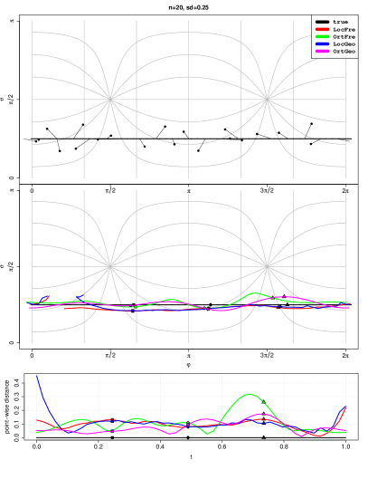
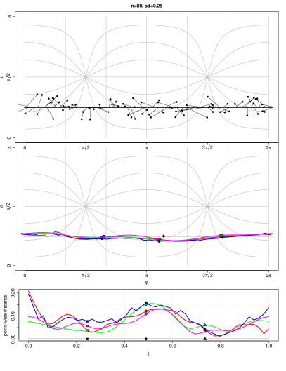
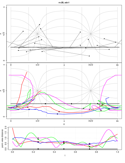
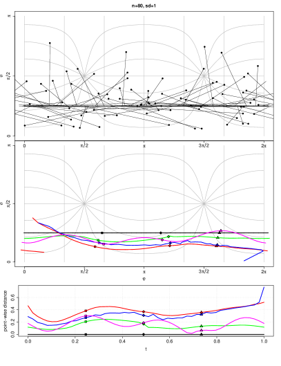
Figure 1: For the simple curve, we sample $n\in\{20,80\}$ observations with contracted uniform noise of standard deviation $\mathtt{sd}\in\{\frac{1}{4},1\}$ (top plot of each quadrant). Then we apply LocGeo, LocFre, OrtGeo, OrtFre (middle part of each quadrant). The distance of the estimated curve to the true one at each point in time is shown in the plots at the bottom of each quadrant.

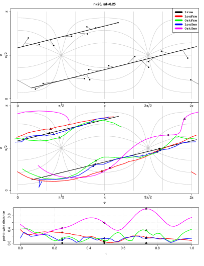
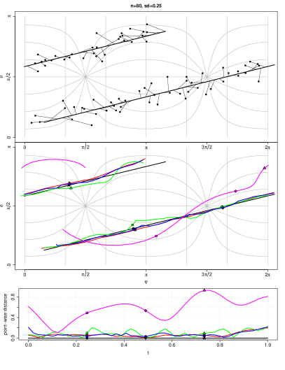
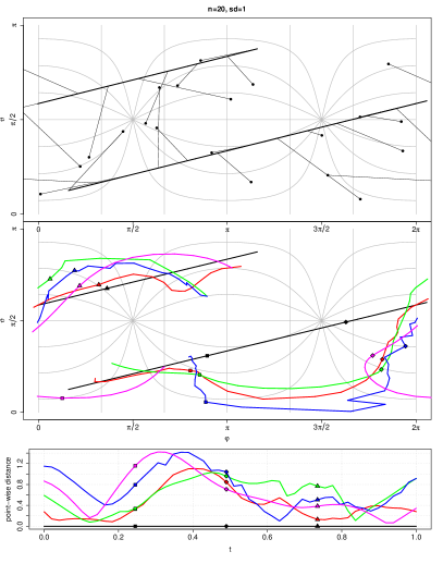
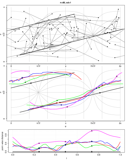
Figure 2: For the spiral, we sample $n\in\{20,80\}$ observations with contracted uniform noise of standard deviation $\mathtt{sd}\in\{\frac{1}{4},1\}$. Then we apply LocGeo, LocFre, OrtGeo, OrtFre. The distance of the estimated curve to the true one at each point in time is shown in the plots at the bottom of each quadrant.

Roughly speaking and judging only from Figure 1 and Figure 2, all estimators seem to perform similarly, except for a worse outcome for OrtGeo on the spiral. In the setting $(n=20,\mathtt{sd}=1)$ the estimators are not able to come close to the true curves.

7.3 Results

We approximate the MISE values in different settings with the simple and the spiral curve. To this end, the simulations are repeated 500 times and the integrated squared errors of these repetitions are averaged. The results are presented in Table 2.

Setting			MISE
$n$	$\mathtt{sd}$	curve	LocFre	OrtFre	LocGeo	OrtGeo
20	0.25	simple	0.02070	0.02410	0.02595	0.01397
80	0.25	simple	0.00731	0.00662	0.00851	0.00361
20	1.00	simple	0.34890	0.39052	0.36356	0.86604
80	1.00	simple	0.12056	0.09350	0.11026	0.09228
20	0.25	spiral	0.02899	0.05902	0.03268	0.38623
80	0.25	spiral	0.00900	0.01534	0.01008	0.37191
20	1.00	spiral	0.56768	0.52354	0.54786	0.91824
80	1.00	spiral	0.15185	0.14662	0.14677	0.47189

Table 2: Approximated MISE values for nonparametric regression methods. The colors give a visual indication of the MISE value of the given methods divided by the best MISE value in the row.

The more reliable analysis of the approximated MISE-values confirms that all estimators behave similar, except OrtGeo, which has some bad outcomes. This may have several reasons: We were not able to show an error bound for this method and argued that it may be sub-optimal, i.e., it may be inherently worse than the other methods. Furthermore, we do not use cross-validation for OrtGeo, as we do for the other methods, but fix $N=3$. Thus, the comparison might be unfair, because the hyper-parameters are not tuned equally. Lastly, in OrtGeo, we have to numerically solve an 8-dimensional non-convex optimization problem (2 dimensions for each of $\hat{p}$, $\hat{v}_{1}$, $\hat{v}_{2}$, $\hat{v}_{3}$). There are 4 dimensions for LocGeo and 2 for the Fréchet methods, see Table 1. Our program might return values farther away from the optimum in those methods with higher dimensional optimization problems.

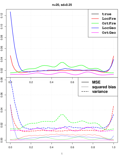
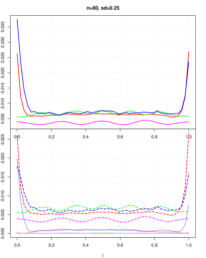
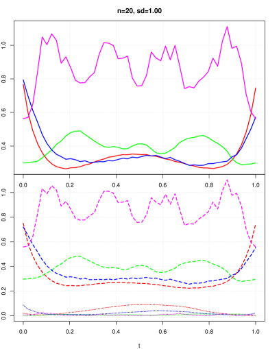
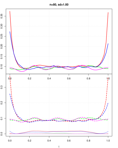
Figure 3: Point-wise MSE, squared bias, and variance for the simple curve.

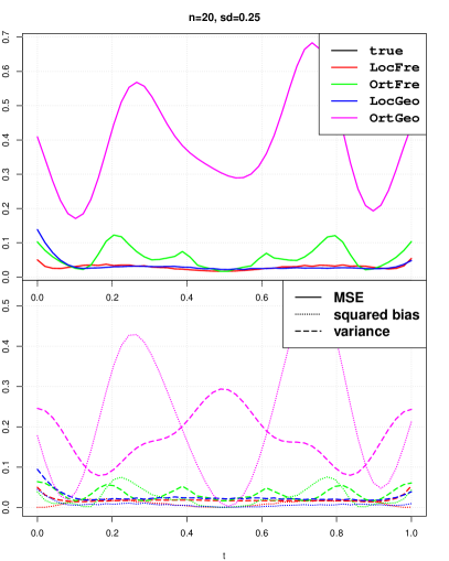
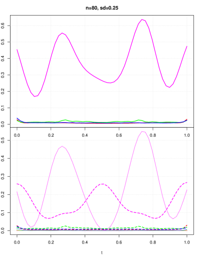
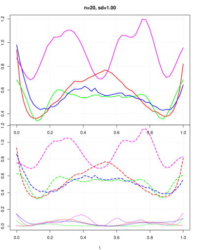
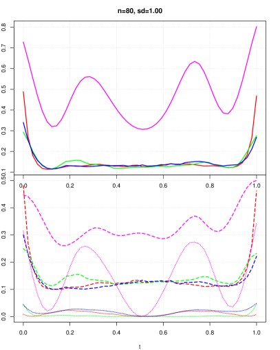
Figure 4: Point-wise MSE, squared bias, and variance for the spiral.

Figure 3 and Figure 4 show the approximated point-wise mean squared error in the upper part of each plot. In the lower part, a point-wise decomposition into a squared bias and a variance term is shown. This decomposition is not straight forward in curved spaces: We calculate the Fréchet mean $\bar{m}_{t}$ of our repetitions $(\hat{m}_{t}^{j})_{j=1,\dots,500}$. The dotted line in each plot is $t\mapsto d(\bar{m}_{t},m_{t})^{2}=:\mathsf{Bias}^{2}_{t}$. The dashed line is $\frac{1}{500}\sum_{j=1}^{500}d(\bar{m}_{t},\hat{m}_{t}^{j})^{2}=:\mathsf{Var}_{t}$. But, in nonstandard spaces, there is no guarantee that $\frac{1}{500}\sum_{j=1}^{500}d(m_{t},\hat{m}_{t}^{j})^{2}=:\mathsf{MSE}_{t}=\mathsf{Bias}^{2}_{t}+\mathsf{Var}_{t}$. Still this decomposition is valuable. It shows that OrtGeo is an unbiased estimator of the simple curve, which is not surprising as OrtGeo with $N=3$ is a parametric estimator and the simple curve is in its model space. On the spiral the estimators suffer from boundary effects. On the simple curve this only affects the local estimators as this curve is periodic and does not have a boundary for the trigonometric estimators.

Appendix A Proofs

Recall the general metric space model. Let $(\mathcal{Q},d)$ be a metric space. For $t\in[0,1]$, let $Y_{t}$ be a $\mathcal{Q}$-valued random variable with finite second moment, i.e., $\mathbb{E}[d(Y_{t},q)^{2}]<\infty$ for all $t\in[0,1]$ and $q\in\mathcal{Q}$. Let the regression function $m\colon[0,1]\to\mathcal{Q}$ be a minimizer $m_{t}\in\operatorname*{arg\,min}_{q\in\mathcal{Q}}\mathbb{E}[d(Y_{t},q)^{2}]$. We consider nonparametric estimators which have access to following data: Let $x_{i}=\frac{i}{n}$ and let $(y_{i})_{i=1,\dots,n}$ be independent random variables with values in $\mathcal{Q}$ such that $y_{i}$ has the same distribution as $Y_{x_{i}}$.

We introduce some further notation. Define

$$\overline{q,\!p} :=d(q,p)\,,$$

$$\lozenge(y,z,q,p) :=d(y,q)^{2}-d(y,p)^{2}-d(z,q)^{2}+d(z,p)^{2}\,,$$

$$\mathfrak{a}(y,z) :=\sup_{q,p\in\mathcal{Q},q\neq p}\frac{\lozenge(y,z,q,p)}{d(q,p)}\,.$$

A.1 LocFre

A.1.1 A General Result

To prove the theorems from section 2 concerning the LocFre estimator, we show a more general results first.

For $a>0$, define $\lfloor a\rfloor$ as the largest integer strictly smaller than $a$. The Hölder class $\Sigma(\beta,L)$ for $\beta,L>0$ is defined as the set of $\lfloor\beta\rfloor$-times continuously differentiable functions $f\colon[0,1]\to\mathbb{R}$ with $\left|f^{(\lfloor\beta\rfloor)}(t)-f^{(\lfloor\beta\rfloor)}(x)\right|\leq L\left|x-t\right|^{\beta-\lfloor\beta\rfloor}$ for all $x,t\in[0,1]$.

Assumptions 5.

• VarIneq: There is $C_{\mathsf{Vlo}}\in[1,\infty)$ such that $C_{\mathsf{Vlo}}^{-1}\,\overline{q,\!m_{t}}^{2}\leq\mathbb{E}[d(Y_{t},q)^{2}-d(Y_{t},m_{t})^{2}]$ for all $q\in\mathcal{Q}$ and $t\in[0,1]$.

• Entropy: There are $C_{\mathsf{Ent}}\in[1,\infty)$ and $\alpha\in[1,2)$ such that

  $$\gamma_{2}(\mathcal{B},d)\leq C_{\mathsf{Ent}}\max(\operatorname{\mathsf{diam}}(\mathcal{B},d),\operatorname{\mathsf{diam}}(\mathcal{B},d)^{\alpha})$$

  for all $\mathcal{B}\subseteq\mathcal{Q}$, where $\gamma_{2}$ is the measure of entropy defined 1.

• Moment: There are $\kappa>\frac{2}{2-\alpha}$ and $C_{\mathsf{Mom}}\in[1,\infty)$ such that $\mathbb{E}[d(Y_{t},m_{t})^{\kappa}]^{\frac{1}{\kappa}}\leq C_{\mathsf{Mom}}$ for all $t\in[0,1]$.

• Kernel: There are $C_{\mathsf{Kmi}},C_{\mathsf{Kma}}\in[1,\infty)$ such that

  $$C_{\mathsf{Kmi}}^{-1}\mathds{1}_{[-\frac{1}{2},\frac{1}{2}]}(x)\leq K(x)\leq C_{\mathsf{Kma}}\mathds{1}_{[-1,1]}(x)$$

  for all $x\in\mathbb{R}$.

• HölderSmoothDensity: The function $[0,1]\to\mathcal{Q},\,t\mapsto m_{t}$ is continuous. Let $C_{\mathsf{Len}}\in[1,\infty)$ such that $\sup_{s,t\in[0,1]}d(m_{s},m_{t})\leq C_{\mathsf{Len}}$. Let $\mu$ be a probability measure on $\mathcal{Q}$. Let $C_{\mathsf{Int}}\in[1,\infty)$ such that $\int\overline{y,\!m_{0}}^{2}\mu(\mathrm{d}y)\leq C_{\mathsf{Int}}$. Let $y\to\rho(y|t)$ be the $\mu$-density of $Y_{t}$. Let $\beta>0$ with $\ell=\lfloor\beta\rfloor$. For $\mu$-almost all $y\in\mathcal{Q}$, there is $L(y)\geq 0$ such that $t\mapsto\rho(y|t)\in\Sigma(\beta,L(y))$. Furthermore, there is a constant $C_{\mathsf{SmD}}>0$, $\int L(y)^{2}\mathrm{d}\mu(y)\leq C_{\mathsf{SmD}}^{2}$.

• BiasMoment: Define $H(q,p)=(\int\left(\overline{y,\!q}+\overline{y,\!p}\right)^{2}\mu(\mathrm{d}y))^{\frac{1}{2}}$. There is $C_{\mathsf{Bom}}\in[1,\infty)$ such that $\mathbb{E}[H(\hat{m}_{t},m_{t})^{\kappa}]^{\frac{1}{\kappa}}\leq C_{\mathsf{Bom}}$ for all $t\in[0,1]$.

Theorem 7 (LocFre General).

Assume HölderSmoothDensity, BiasMoment, Kernel, VarIneq, Entropy, Moment. Let $\ell=\lfloor\beta\rfloor$. Then, for $t\in[0,1]$, $n\geq c$, and $h\geq\frac{c}{n}$, the local polynomial Fréchet estimator $\hat{m}_{t}$ of order $\ell$ fulfills,

$$\mathbb{E}\left[\overline{m_{t},\!\hat{m}_{t}}^{2}\right]\leq C_{1}\left(h^{2\beta}+h^{\frac{2\beta}{2-\alpha}}\right)+C_{2}\left((nh)^{-1}+(nh)^{-\frac{1}{2-\alpha}}\right)\,,$$

where $C_{1}=c_{\alpha,\kappa}\left(C_{\mathsf{Vlo}}C_{\mathsf{Kmi}}C_{\mathsf{Kma}}C_{\mathsf{SmD}}C_{\mathsf{Bom}}\right)^{\frac{2}{2-\alpha}}$ and $C_{2}=c_{\alpha,\kappa}\left(C_{\mathsf{Vlo}}C_{\mathsf{Mom}}C_{\mathsf{Ent}}C_{\mathsf{Kmi}}^{2}C_{\mathsf{Kma}}^{2}\right)^{\frac{2}{2-\alpha}}$.

To prove Theorem 7, We first apply the variance inequality to relate a bound on the objective functions to a bound on the minimizers. The required uniform bound on the objective functions can be split into a bias and a variance part, which are bounded separately thereafter. Then, these results are put together in the application of a peeling device, which is used to bound the tail probabilities of the error. Integrating the tails leads to the required bounds in expectation.

A.1.2 Proof of the General Result

Kernel. First we state some properties of the weights $w_{i,t}$ to be used later.

Lemma 1 ([27, Proposition 1.12, Lemma 1.3, Lemma 1.5]).

Assume Kernel. Let $f\colon\mathbb{R}\to\mathbb{R}$ be a polynomial of degree $\leq\ell$. Then

$$w_{i,t}=0\text{ if $\left|x_{i}-t\right|>h$}\,, \sum_{i=1}^{n}w_{i,t}=1\,, \sum_{i=1}^{n}f(x_{i})w_{i,t}=f(t)\,,$$

$$\left|w_{i,t}\right|\leq c\frac{C_{\mathsf{Kmi}}C_{\mathsf{Kma}}}{nh}\,, \sum_{i=1}^{n}|w_{i,t}|\leq cC_{\mathsf{Kmi}}C_{\mathsf{Kma}}\,, \sum_{i=1}^{n}w_{i,t}^{2}\leq c\frac{C_{\mathsf{Kmi}}^{2}C_{\mathsf{Kma}}^{2}}{nh}\,.$$

for all $t\in[0,1]$, $h\geq\frac{c}{n}$, $n\geq c$.

Proof.

The first statement is due to the bounded support of the kernel. For the other statements in the first row, see [27, Proposition 1.12]. The next two bounds follow from [27, Lemma 1.3, Lemma 1.5]. The last bound is a consequence of the previous two. ∎

Variance Inequality and Split. We define following notation for the objective functions

$$\hat{F}_{t}(q) =\sum_{i=1}^{n}w_{i,t}d(y_{i},q)^{2} \hat{F}_{t}(q,p) =\hat{F}_{t}(q)-\hat{F}_{t}(p)\,,$$

$$\bar{F}_{t}(q) =\sum_{i=1}^{n}w_{i,t}\mathbb{E}[d(y_{i},q)^{2}] \bar{F}_{t}(q,p) =\bar{F}_{t}(q)-\bar{F}_{t}(p)\,,$$

$$F_{t}(q) =\mathbb{E}[d(Y_{t},q)^{2}] F_{t}(q,p) =F_{t}(q)-F_{t}(p)\,.$$

Using VarIneq and the minimizing property of $\hat{m}_{t}$ we obtain

$$C_{\mathsf{Vlo}}^{-1}d(\hat{m}_{t},m_{t})^{\alpha} \leq F_{t}(\hat{m}_{t},m_{t})$$

$$\leq F_{t}(\hat{m}_{t},m_{t})-\hat{F}_{t}(\hat{m}_{t},m_{t})$$

$$=\left(F_{t}(\hat{m}_{t},m_{t})-\bar{F}_{t}(\hat{m}_{t},m_{t})\right)+\left(\bar{F}_{t}(\hat{m}_{t},m_{t})-\hat{F}_{t}(\hat{m}_{t},m_{t})\right)$$

The first parenthesis represents the bias part, the second one the variance part. We will bound the former using HölderSmoothDensity, the later by an empirical process argument.

Variance. Define

$$Z_{i}(q) =w_{i,t}\left(d(y_{i},q)^{2}-d(y_{i},m_{t})^{2}\right)-\mathbb{E}\left[w_{i,t}\left(d(y_{i},q)^{2}-d(y_{i},m_{t})^{2}\right)\right]\,.$$

Then $Z_{1},\dots,Z_{n}$ are independent and centered processes with $Z_{i}(m_{t})=0$. They are integrable due to Moment. By the definition of $\mathfrak{a}$,

$$\left|Z_{i}(q)-Z_{i}(p)-Z_{i}^{\prime}(q)+Z_{i}^{\prime}(p)\right|\leq\left|w_{i,t}\right|\mathfrak{a}(y_{i},y_{i}^{\prime})d(q,p)\,,$$

where $Z_{i}(q)^{\prime}$ and $y_{i}^{\prime}$ are independent copies of $Z_{i}(q)$ and $y_{i}$, respectively. Theorem 10 yields

$$\mathbb{E}\left[\sup_{q\in\operatorname{\mathrm{B}}(m_{t},d,\delta)}\left\nonscript\;\middle|\nonscript\;\bar{F}_{t}(q,m_{t})-\hat{F}_{t}(q,m_{t})\right\nonscript\;\middle|\nonscript\;^{\kappa}\right]=\mathbb{E}\left[\sup_{q\in\operatorname{\mathrm{B}}(m_{t},d,\delta)}\left\nonscript\;\middle|\nonscript\;\sum_{i=1}^{n}Z_{i}(q)\right\nonscript\;\middle|\nonscript\;^{\kappa}\right]$$

$$\leq c_{\kappa}\left(\mathbb{E}\left[\left(\sum_{i=1}^{n}w_{i,t}^{2}\mathfrak{a}(y_{i},y_{i}^{\prime})^{2}\right)^{\frac{\kappa}{2}}\right]^{\frac{1}{\kappa}}\gamma_{2}(\operatorname{\mathrm{B}}(m_{t},d,\delta),d)\right)^{\kappa}$$

for a constant $c_{\kappa}$ depending only on $\kappa$. Define $W=\sum_{i=1}^{n}w_{i,t}^{2}$ and $v_{i}=w_{i,t}^{2}/W$. We apply Moment,

$$\mathbb{E}\left[\left(\sum_{i=1}^{n}w_{i,t}^{2}\mathfrak{a}(y_{i},y_{i}^{\prime})^{2}\right)^{\frac{\kappa}{2}}\right] =\mathbb{E}\left[\left(W\sum_{i=1}^{n}v_{i}\mathfrak{a}(y_{i},y_{i}^{\prime})^{2}\right)^{\frac{\kappa}{2}}\right]$$

$$\leq\mathbb{E}\left[W^{\frac{\kappa}{2}}\sum_{i=1}^{n}v_{i}\mathfrak{a}(y_{i},y_{i}^{\prime})^{\kappa}\right]$$

$$=W^{\frac{\kappa}{2}}\sum_{i=1}^{n}v_{i}\mathbb{E}\left[\mathfrak{a}(y_{i},y_{i}^{\prime})^{\kappa}\right]$$

$$\leq W^{\frac{\kappa}{2}}C_{\mathsf{Mom}}^{\kappa}\,.$$

By 1, $W\leq cC_{\mathsf{Kmi}}^{2}C_{\mathsf{Kma}}^{2}(nh)^{-1}$. By Entropy, $\gamma_{2}(\operatorname{\mathrm{B}}(m_{t},d,\delta),d)\leq C_{\mathsf{Ent}}\max(\delta,\delta^{\alpha})$. Thus,

$$\mathbb{E}\left[\sup_{q\in\operatorname{\mathrm{B}}(m_{t},d,\delta)}\left\nonscript\;\middle|\nonscript\;\bar{F}_{t}(q,m_{t})-\hat{F}_{t}(q,m_{t})\right\nonscript\;\middle|\nonscript\;^{\kappa}\right]\leq c_{\kappa}\left(C_{\mathsf{Mom}}C_{\mathsf{Ent}}C_{\mathsf{Kmi}}^{2}C_{\mathsf{Kma}}^{2}\max(\delta,\delta^{\alpha})(nh)^{-\frac{1}{2}}\right)^{\kappa}\,.$$

Bias. As $\sum_{i=1}^{n}w_{i,t}=1$ (1), we have

$$F_{t}(q,m_{t})-\bar{F}_{t}(q,m_{t})=\sum_{i=1}^{n}w_{i,t}\mathbb{E}[\lozenge(Y_{t},y_{i},q,m_{t})]\,.$$

Using the $\mu$-density $y\mapsto\rho(y|t)$ of $Y_{t}$, we can write $\mathbb{E}[\overline{Y_{t},\!q}^{2}-\overline{Y_{t},\!p}^{2}]=$ $\int\left(\overline{y,\!q}^{2}-\overline{y,\!p}^{2}\right)\rho(y|t)\mathrm{d}\mu(y)$. By HölderSmoothDensity, $t\mapsto\rho(y|t)\in\Sigma(\beta,L(y))$. Thus, there are $a_{k}(y)$ such that $\rho(y|x)=R_{y}(x,x_{0})+\sum_{k=0}^{\ell}a_{k}(y)(x-x_{0})^{k}$ with $\left|R_{y}(x,x_{0})\right|\leq L(y)\left|x-x_{0}\right|^{\beta}$. Using that the weights annihilate polynomials of order $\ell$ [27, equation (1.68)], we obtain

$$\sum_{i=1}^{n}w_{i,t}\mathbb{E}[\lozenge(Y_{t},y_{i},q,p)] =\int\sum_{i=1}^{n}w_{i,t}\left(\overline{y,\!q}^{2}-\overline{y,\!p}^{2}\right)\left(\rho(y|t)-\rho(y|x_{i})\right)\mathrm{d}\mu(y)$$

$$=\int\sum_{i=1}^{n}w_{i,t}\left(\overline{y,\!q}^{2}-\overline{y,\!p}^{2}\right)R_{y}(t,x_{i})\mathrm{d}\mu(y)$$

$$\leq\int\sum_{i=1}^{n}\left|w_{i,t}\right|\left|\overline{y,\!q}^{2}-\overline{y,\!p}^{2}\right|\left|R_{y}(t,x_{i})\right|\mathrm{d}\mu(y)\,.$$

It holds

$$\left|\overline{y,\!q}^{2}-\overline{y,\!p}^{2}\right|\left|R_{y}(x,x_{0})\right| \leq\overline{q,\!p}\left|x-x_{0}\right|^{\beta}\left(\overline{y,\!q}+\overline{y,\!p}\right)L(y)\,.$$

Together with $\sum_{i=1}^{n}\left|w_{i,t}\right|\leq cC_{\mathsf{Kmi}}C_{\mathsf{Kma}}$ from 1, we obtain

$$\left|\sum_{i=1}^{n}w_{i,t}\mathbb{E}[\lozenge(Y_{t},y_{i},q,p)]\right|\leq cC_{\mathsf{Kmi}}C_{\mathsf{Kma}}\,\overline{q,\!p}\,h^{\beta}\int\left(\overline{y,\!q}+\overline{y,\!p}\right)L(y)\mathrm{d}\mu(y)$$

Recall $H(q,p)=\left(\int\left(\overline{y,\!q}+\overline{y,\!p}\right)^{2}\mu(\mathrm{d}y)\right)^{\frac{1}{2}}$. By the Cauchy–Schwartz inequality and HölderSmoothDensity,

$$\int\left(\overline{y,\!q}+\overline{y,\!p}\right)L(y)\mathrm{d}\mu(y)\leq H(q,p)\left(\int L(y)^{2}\mathrm{d}\mu(y)\right)^{\frac{1}{2}}\leq H(q,p)C_{\mathsf{SmD}}\,.$$

Thus,

$$F_{t}(q,m_{t})-\bar{F}_{t}(q,m_{t})\leq cC_{\mathsf{Kmi}}C_{\mathsf{Kma}}C_{\mathsf{SmD}}\,\overline{q,\!p}\,h^{\beta}H(q,m_{t})$$ (45)

BiasMoment states $\mathbb{E}[H(\hat{m}_{t},m_{t})^{\kappa}]^{\frac{1}{\kappa}}\leq C_{\mathsf{Bom}}$. Finally we obtain

$$\mathbb{E}\left[\left\nonscript\;\middle|\nonscript\;F_{t}(\hat{m}_{t},m_{t})-\bar{F}_{t}(\hat{m}_{t},m_{t})\right\nonscript\;\middle|\nonscript\;^{\kappa}\mathds{1}_{[0,\delta]}(d(\hat{m}_{t},m_{t}))\right]^{\frac{1}{\kappa}}$$

$$\leq\mathbb{E}\left[\left\nonscript\;\middle|\nonscript\;cC_{\mathsf{Kmi}}C_{\mathsf{Kma}}C_{\mathsf{SmD}}d(\hat{m}_{t},m_{t})H(\hat{m}_{t},m_{t})h^{\beta}\right\nonscript\;\middle|\nonscript\;^{\kappa}\mathds{1}_{[0,\delta]}(d(\hat{m}_{t},m_{t}))\right]^{\frac{1}{\kappa}}$$

$$\leq cC_{\mathsf{Kmi}}C_{\mathsf{Kma}}C_{\mathsf{SmD}}C_{\mathsf{Bom}}\delta h^{\beta}\,.$$

Peeling. For $\delta>0$ define

$$\Delta_{\delta}(q,p)=\left(\left|F_{t}(q,p)-\bar{F}_{t}(q,p)\right|+\left|\bar{F}_{t}(q,p)-\hat{F}_{t}(q,p)\right|\right)\mathds{1}_{[0,\delta]}(d(q,p))\,.$$

Recall that the variance inequality implies

$$C_{\mathsf{Vlo}}^{-1}d(\hat{m}_{t},m_{t})^{2}\leq\left(F_{t}(\hat{m}_{t},m_{t})-\bar{F}_{t}(\hat{m}_{t},m_{t})\right)+\left(\bar{F}_{t}(\hat{m}_{t},m_{t})-\hat{F}_{t}(\hat{m}_{t},m_{t})\right)\,.$$

Let $0<a<b<\infty$. The inequality above and Markov’s inequality yield

$$\mathbb{P}\mathopen{}\left(d(\hat{m}_{t},m_{t})\in[a,b]\right)\mathclose{}\leq\mathbb{P}\mathopen{}\left(a^{2}\leq C_{\mathsf{Vlo}}\Delta_{b}(\hat{m}_{t},m_{t})\right)\mathclose{}\leq\frac{C_{\mathsf{Vlo}}^{\kappa}\mathbb{E}[\Delta_{b}(\hat{m}_{t},m_{t})^{\kappa}]}{a^{2\kappa}}\,.$$

Our previous consideration allow us the bound the expectation by a variance and a bias term:

$$\mathbb{E}[\Delta_{\delta}(\hat{m}_{t},m_{t})^{\kappa}] \leq 2^{\kappa-1}\Bigg{(}\mathbb{E}\left[\left\nonscript\;\middle|\nonscript\;F_{t}(\hat{m}_{t},m_{t})-\bar{F}_{t}(\hat{m}_{t},m_{t})\right\nonscript\;\middle|\nonscript\;^{\kappa}\mathds{1}_{[0,\delta]}(d(\hat{m}_{t},m_{t}))\right]$$

$$\quad+\mathbb{E}\left[\sup_{q\in\operatorname{\mathrm{B}}(m_{t},d,\delta)}\left\nonscript\;\middle|\nonscript\;\bar{F}_{t}(q,m_{t})-\hat{F}_{t}(q,m_{t})\right\nonscript\;\middle|\nonscript\;^{\kappa}\right]\Bigg{)}$$

$$\leq c_{\kappa}\left(C_{\mathsf{Kmi}}C_{\mathsf{Kma}}C_{\mathsf{SmD}}C_{\mathsf{Bom}}h^{\beta}+C_{\mathsf{Mom}}C_{\mathsf{Ent}}C_{\mathsf{Kmi}}^{2}C_{\mathsf{Kma}}^{2}(nh)^{-\frac{1}{2}}\right)^{\kappa}\max(\delta,\delta^{\alpha})^{\kappa}\,.$$

We are now prepared to apply peeling (also called slicing): Let $s>0$. Set $A=C_{\mathsf{Vlo}}C_{\mathsf{Kmi}}C_{\mathsf{Kma}}C_{\mathsf{SmD}}C_{\mathsf{Bom}}h^{\beta}+C_{\mathsf{Vlo}}C_{\mathsf{Mom}}C_{\mathsf{Ent}}cC_{\mathsf{Kmi}}^{2}C_{\mathsf{Kma}}^{2}(nh)^{-\frac{1}{2}}$. It holds

$$\mathbb{P}\mathopen{}\left(d(\hat{m}_{t},m_{t})>s\right)\mathclose{} \leq\sum_{k=0}^{\infty}\mathbb{P}\mathopen{}\left(d(\hat{m}_{t},m_{t})\in[2^{k}s,2^{k+1}s]\right)\mathclose{}$$

$$\leq\sum_{k=0}^{\infty}\frac{c_{\kappa}A^{\kappa}\max(2^{k+1}s,(2^{k+1}s)^{\alpha})^{\kappa}}{(2^{k}s)^{2\kappa}}$$

$$\leq c_{\kappa}A^{\kappa}\left(s^{-\kappa}+s^{-\kappa(2-\alpha)}\right)\sum_{k=0}^{\infty}2^{-k\kappa(2-\alpha)}$$

$$\leq c_{\kappa}A^{\kappa}\left(s^{-\kappa}+s^{-\kappa(2-\alpha)}\right)\,.$$

We integrate this tail bound to bound the expectation. For this we require $\kappa>\frac{2}{2-\alpha}$. Set $B=c_{\kappa}A^{\kappa}$, then

$$\mathbb{E}[d(\hat{m}_{t},m_{t})^{2}] =2\int_{0}^{\infty}s\mathbb{P}\mathopen{}\left(d(\hat{m}_{t},m_{t})>s\right)\mathclose{}\mathrm{d}s$$

$$\leq 2\int_{0}^{\infty}s\min\!\left(1,B\left(s^{-\kappa}+s^{-\kappa(2-\alpha)}\right)\right)\mathrm{d}s$$

$$\leq 2\int_{0}^{\infty}s\min\!\left(1,Bs^{-\kappa}\right)\mathrm{d}s+2\int_{0}^{\infty}s\min\!\left(1,Bs^{-\kappa(2-\alpha)}\right)\mathrm{d}s\,.$$

For the first summand,

$$2\int_{0}^{\infty}s\min\!\left(1,Bs^{-\kappa}\right)\mathrm{d}s =2\int_{0}^{B^{\frac{1}{\kappa}}}s\,\mathrm{d}s+2B\int_{B^{\frac{1}{\kappa}}}^{\infty}s^{1-\kappa}\mathrm{d}s$$

$$=B^{\frac{2}{\kappa}}+\frac{2B}{\kappa-2}B^{\frac{2-\kappa}{\kappa}}$$

$$=\frac{\kappa}{\kappa-2}B^{\frac{2}{\kappa}}\,.$$

Similarly,

$$2\int_{0}^{\infty}s\min\!\left(1,Bs^{-\kappa(2-\alpha)}\right)\mathrm{d}s\leq\frac{\kappa(2-\alpha)}{\kappa(2-\alpha)-2}B^{\frac{2}{\kappa(2-\alpha)}}$$

Thus,

$$\mathbb{E}[d(\hat{m}_{t},m_{t})^{2}] \leq c_{\kappa}\left(A^{2}+A^{\frac{2}{2-\alpha}}\right)$$

$$\leq c_{\alpha,\kappa}\left(C_{\mathsf{Vlo}}C_{\mathsf{Kmi}}C_{\mathsf{Kma}}C_{\mathsf{SmD}}C_{\mathsf{Bom}}\right)^{\frac{2}{2-\alpha}}\left(h^{2\beta}+h^{\frac{2\beta}{2-\alpha}}\right)+$$

$$\hphantom{\leq}\ \,c_{\alpha,\kappa}\left(C_{\mathsf{Vlo}}C_{\mathsf{Mom}}C_{\mathsf{Ent}}C_{\mathsf{Kmi}}^{2}C_{\mathsf{Kma}}^{2}\right)^{\frac{2}{2-\alpha}}\left((nh)^{-1}+(nh)^{-\frac{1}{2-\alpha}}\right)\,.$$

A.1.3 Main Theorems

We use Theorem 7 to prove the two main theorems concerning LocFre. Recall $H(q,p)=\left(\int\left(\overline{y,\!q}+\overline{y,\!p}\right)^{2}\mu(\mathrm{d}y)\right)^{\frac{1}{2}}$.

Proof of Theorem 1.

We want to apply Theorem 7 with $\alpha=1$. As $\operatorname{\mathsf{diam}}(\mathcal{Q},d)<\infty$, $H(q,p)\leq 2\operatorname{\mathsf{diam}}(\mathcal{Q})$ for all $q,p\in\mathcal{Q}$, and we can set $C_{\mathsf{Bom}}=2\,\operatorname{\mathsf{diam}}(\mathcal{Q},d)$. Furthermore, $\overline{y,\!q}^{2}-\overline{y,\!p}^{2}-\overline{z,\!q}^{2}+\overline{z,\!p}^{2}\leq 4\overline{q,\!p}\operatorname{\mathsf{diam}}(\mathcal{Q},d)$. Thus, $\mathfrak{a}(y,z)\leq 4\operatorname{\mathsf{diam}}(\mathcal{Q},d)$ and we can choose $C_{\mathsf{Mom}}=4\operatorname{\mathsf{diam}}(\mathcal{Q},d)$. Lastly, we may integrate the inequality $\mathbb{E}[\overline{m_{t},\!\hat{m}_{t}}^{2}]\leq C_{1}h^{2\beta}+C_{2}(nh)^{-1}$ with respect to $t$ to obtain the bound for the mean integrated squared error. ∎

Proposition 3.

Let $\mathcal{Q}$ be a Hadamard space. Assume HölderSmoothDensity, Kernel, Moment. To fulfill BiasMoment, we can choose

$$C_{\mathsf{Bom}}=c_{\kappa}C_{\mathsf{Mom}}C_{\mathsf{Kmi}}C_{\mathsf{Kma}}C_{\mathsf{Len}}C_{\mathsf{Int}}\,.$$

Proof of 3.

Using the triangle inequality

$$H(q,p)^{2} =\int\left(\overline{y,\!q}+\overline{y,\!p}\right)^{2}\mu(\mathrm{d}y)$$

$$\leq\int\left(\overline{q,\!p}+2\overline{y,\!p}\right)^{2}\mu(\mathrm{d}y)$$

$$\leq 2\int\overline{q,\!p}^{2}+4\overline{y,\!p}^{2}\mu(\mathrm{d}y)$$

$$\leq 2\overline{q,\!p}^{2}+8\int\overline{y,\!p}^{2}\mu(\mathrm{d}y)$$

as $\mu$ is a probability measure.

$$\mathbb{E}[H(\hat{m}_{t},m_{t})^{\kappa}]^{\frac{1}{\kappa}} \leq\mathbb{E}\left[\left(2\overline{\hat{m}_{t},\!m_{t}}^{2}+8\int\overline{y,\!m_{t}}^{2}\mu(\mathrm{d}y)\right)^{\frac{\kappa}{2}}\right]^{\frac{1}{\kappa}}$$

$$\leq c_{\kappa}\left(\mathbb{E}\left[\overline{\hat{m}_{t},\!m_{t}}^{\kappa}\right]^{\frac{1}{\kappa}}+\left(\int\overline{y,\!m_{0}}^{2}\mu(\mathrm{d}y)\right)^{\frac{1}{2}}+\overline{m_{t},\!m_{0}}\right)$$

$$\leq c_{\kappa}\left(\mathbb{E}\left[\overline{\hat{m}_{t},\!m_{t}}^{\kappa}\right]^{\frac{1}{\kappa}}+C_{\mathsf{Int}}+C_{\mathsf{Len}}\right)\,.$$

Next, we will bound $\mathbb{E}[\overline{m_{t},\!\hat{m}_{t}}^{\kappa}]$. Let $W=\sum_{i=1}^{n}\left|w_{i,t}\right|$. First, as VarIneq holds in Hadamard spaces with $C_{\mathsf{Vlo}}=1$, $\lozenge(y,z,q,p)\leq 2\overline{y,\!z}\,\overline{q,\!p}$ in Hadamard spaces, and the minimizing property of $\hat{m}_{t}$,

$$\overline{m_{t},\!\hat{m}_{t}}^{2} \leq F_{t}(\hat{m}_{t},m_{t})$$

$$\leq F_{t}(\hat{m}_{t},m_{t})-\hat{F}_{t}(\hat{m}_{t},m_{t})$$

$$=\sum_{i=1}^{n}w_{i,t}\mathbb{E}[\lozenge(Y_{t},y_{i},m_{t},\hat{m}_{t})\nonscript\;|\nonscript\;y_{1\dots n}]$$

$$\leq 2\sum_{i=1}^{n}\left|w_{i,t}\right|\overline{\hat{m}_{t},\!m_{t}}\,\mathbb{E}[d(Y_{t},y_{i})\nonscript\;|\nonscript\;y_{i}]\,.$$

Thus,

$$\overline{m_{t},\!\hat{m}_{t}}\leq\sum_{i=1}^{n}\left|w_{i,t}\right|\mathbb{E}[d(Y_{t},y_{i})\nonscript\;|\nonscript\;y_{i}]$$

With Jensen’s inequality

$$\mathbb{E}[\overline{m_{t},\!\hat{m}_{t}}^{\kappa}] \leq\mathbb{E}\left[\left(\sum_{i=1}^{n}\left\nonscript\;\middle|\nonscript\;w_{i,t}\right\nonscript\;\middle|\nonscript\;\mathbb{E}[d(Y_{t},y_{i})\nonscript\;|\nonscript\;y_{i}]\right)^{\kappa}\right]$$

$$=W^{\kappa}\mathbb{E}\left[\left(\sum_{i=1}^{n}\frac{\left\nonscript\;\middle|\nonscript\;w_{i,t}\right\nonscript\;\middle|\nonscript\;}{W}\mathbb{E}[d(Y_{t},y_{i})\nonscript\;|\nonscript\;y_{i}]\right)^{\kappa}\right]$$

$$\leq W^{\kappa}\sum_{i=1}^{n}\frac{\left|w_{i,t}\right|}{W}\mathbb{E}\left[\mathbb{E}[d(Y_{t},y_{i})\nonscript\;|\nonscript\;y_{i}]^{\kappa}\right]$$

$$\leq W^{\kappa}\sum_{i=1}^{n}\frac{\left|w_{i,t}\right|}{W}\mathbb{E}[d(Y_{t},y_{i})^{\kappa}]$$

$$\leq W^{\kappa}\sup_{s,t\in[0,1]}\mathbb{E}\left[d(Y_{t},Y^{\prime}_{s})^{\kappa}\right]\,.$$

As $d$ is a metric,

$$\mathbb{E}\left[d(Y_{t},Y^{\prime}_{s})^{\kappa}\right] \leq\mathbb{E}\left[\left(d(Y_{t},m_{t})+d(m_{t},m_{s})+d(m_{s},Y^{\prime}_{s})\right)^{\kappa}\right]$$

$$\leq 3^{\kappa}\left(2\sup_{t\in[0,1]}\mathbb{E}\left[d(Y_{t},m_{t})^{\kappa}\right]+d(m_{t},m_{s})^{\kappa}\right)$$

$$\leq c_{\kappa}\left(C_{\mathsf{Mom}}^{\kappa}+C_{\mathsf{Len}}^{\kappa}\right)\,.$$

1 shows $W\leq cC_{\mathsf{Kmi}}C_{\mathsf{Kma}}$. This completes the proof. ∎

Proof of Theorem 2.

We want to apply Theorem 7. VarIneq holds in Hadamard spaces with $C_{\mathsf{Vlo}}=1$. Furthermore, the quadruple inequality in Hadamard spaces yields $\mathfrak{a}(y,z)=2d(y,z)$, which allows to state the moment condition with respect to $d$ instead of $\mathfrak{a}$. We bound $\mathbb{E}[H(\hat{m}_{t},m_{t})^{\kappa}]^{\frac{1}{\kappa}}\leq C_{\mathsf{Bom}}$ using

$$C_{\mathsf{Bom}}=c_{\kappa}C_{\mathsf{Mom}}C_{\mathsf{Kmi}}C_{\mathsf{Kma}}C_{\mathsf{Len}}C_{\mathsf{Int}}\,,$$

see 3. Lastly, we may integrate the inequality

$$\mathbb{E}\left[\overline{m_{t},\!\hat{m}_{t}}^{2}\right]\leq C_{1}\left(h^{2\beta}+h^{\frac{2\beta}{2-\alpha}}\right)+C_{2}\left((nh)^{-1}+(nh)^{-\frac{1}{2-\alpha}}\right)$$

with respect to $t$ to obtain the bound for the mean integrated squared error. ∎

A.2 OrtFre

A.2.1 A General Result

We prove a general theorem that implies the main theorems concerning OrtFre.

Assumptions 6.

• VarIneq: There is $C_{\mathsf{Vlo}}\in[1,\infty)$ such that $C_{\mathsf{Vlo}}^{-1}\,\overline{q,\!m_{t}}^{2}\leq\mathbb{E}[\overline{Y_{t},\!q}^{2}-\overline{Y_{t},\!m_{t}}^{2}]$ for all $q\in\mathcal{Q}$ and $t\in[0,1]$.

• Entropy: There are $C_{\mathsf{Ent}}\in[1,\infty)$ and $\alpha\in[1,2)$ such that

  $$\gamma_{2}(\mathcal{B},d)\leq C_{\mathsf{Ent}}\max(\operatorname{\mathsf{diam}}(\mathcal{B},d),\operatorname{\mathsf{diam}}(\mathcal{B},d)^{\alpha})$$

  for all $\mathcal{B}\subseteq\mathcal{Q}$, where $\gamma_{2}$ is the measure of entropy defined 1.

• Moment: There are $\kappa>\frac{2}{2-\alpha}$ and $C_{\mathsf{Mom}}\in[1,\infty)$ such that $\mathbb{E}[d(Y_{t},m_{t})^{\kappa}]^{\frac{1}{\kappa}}\leq C_{\mathsf{Mom}}$ for all $t\in[0,1]$.

• SobolevSmoothDensity: The function $[0,1]\to\mathcal{Q},\,t\mapsto m_{t}$ is continuous. Let $C_{\mathsf{Len}}\in[1,\infty)$ such that $\sup_{s,t\in[0,1]}d(m_{s},m_{t})\leq C_{\mathsf{Len}}$. Let $\mu$ be a probability measure on $\mathcal{Q}$. Let $C_{\mathsf{Int}}\in[1,\infty)$ such that $\int\overline{y,\!m_{0}}^{2}\mu(\mathrm{d}y)\leq C_{\mathsf{Int}}$. For all $t\in[0,1]$, the random variable $Y_{t}$ has a density $y\mapsto\rho(y|t)$ with respect to $\mu$. Let $\beta\geq 1$. For $\mu$-almost all $y\in\mathcal{Y}$, there is $L(y)\geq 0$ such that $t\mapsto\rho(y|t)\in W^{\mathsf{per}}(\beta,L(y))$. Furthermore, there is $C_{\mathsf{SmD}}\in[1,\infty)$ such that $\int L(y)^{2}\mathrm{d}\mu(y)\leq C_{\mathsf{SmD}}^{2}$.

• BiasMoment: Define $H(q,p)=\left(\int\left(\overline{y,\!q}+\overline{y,\!p}\right)^{2}\mu(\mathrm{d}y)\right)^{\frac{1}{2}}$. There is $C_{\mathsf{Bom}}\in[1,\infty)$ such that $\mathbb{E}[H(\hat{m}_{t},m_{t})^{\kappa}]^{\frac{1}{\kappa}}\leq C_{\mathsf{Bom}}$ for all $t\in[0,1]$.

Theorem 8 (OrtFre General).

Assume VarIneq, Entropy with $\alpha=1$, Moment, BiasMoment, SobolevSmoothDensity. Then

$$\mathbb{E}\left[\int_{0}^{1}\overline{m_{t},\!\hat{m}_{t}}^{2}\mathrm{d}t\right]\leq C_{1}\left(N^{-2\beta}+Nn^{1-2\beta}\right)+C_{2}\frac{N}{n}\,,$$

where $C_{1}=c_{\kappa,\beta}C_{\mathsf{Vlo}}^{2}C_{\mathsf{SmD}}^{2}C_{\mathsf{Bom}}^{2}$ and $C_{2}=c_{\kappa,\beta}C_{\mathsf{Vlo}}^{2}C_{\mathsf{Mom}}^{2}C_{\mathsf{Ent}}^{2}$.

The difference of the objective functions is split into three parts in 2. In 3, we use a peeling device and the variance inequality to relate this difference to the distance between the minimizers $\hat{m}_{t}$ and $m_{t}$, which is the quantity to be bounded in the theorem. Of the three parts, two bias related quantities are bounded in 4 and 5 with an auxiliary result in 6. The third part, a variance term, is bounded in 7 via chaining. The bounds on the three parts are summarized in 8. In the end, the integral over $t$ is applied to calculate the mean integrated squared error. Here, the auxiliary result 9 is applied.

A.2.2 Proof of the General Result

For shorter notation define $F_{t}(q,p):=F_{t}(q)-F_{t}(p)$ and $\hat{F}_{t}(q,p):=\hat{F}_{t}(q)-\hat{F}_{t}(p)$. We introduce the Fourier coefficients $\vartheta_{j}(q,p)$ of $t\mapsto F_{t}(q,p)$ with respect to the trigonometric basis

$$\vartheta_{j}(q,p)=\int_{0}^{1}\psi_{j}(x)F_{x}(q,p)\mathrm{d}x$$

such that $F_{t}(q,p)=\sum_{j=1}^{\infty}\vartheta_{j}(q,p)\psi_{j}(t)$ due to SobolevSmoothDensity. Define

$$r_{t}(q,p) =\sum_{k=N+1}^{\infty}\vartheta_{j}(q,p)\psi_{j}(t)\,, F^{r}_{t}(q,p) =\Psi_{N}(t)\!^{\top}\!\frac{1}{n}\sum_{i=1}^{n}\Psi_{N}(x_{i})r_{x_{i}}(q,p)\,,$$

$$\varepsilon_{t}(y,q,p) =F_{t}(q,p)-\left(\overline{y,\!q}^{2}-\overline{y,\!p}^{2}\right)\,, F^{\varepsilon}_{t}(q,p) =\Psi_{N}(t)\!^{\top}\!\frac{1}{n}\sum_{i=1}^{n}\Psi_{N}(x_{i})\varepsilon_{x_{i}}(y_{i},q,p)\,.$$

Lemma 2.

If $N<n$, then

$$F_{t}(q,p)-\hat{F}_{t}(q,p)=r_{t}(q,p)+F^{\varepsilon}_{t}(q,p)-F^{r}_{t}(q,p)\,.$$

Proof of 2.

It holds

$$\frac{1}{n}\sum_{i=1}^{n}\psi_{j}(x_{i})\psi_{\tilde{j}}(x_{i})=\delta_{j\tilde{j}}$$

for $j,\ell\in\left\{1,\dots,n-1\right\}$, see [27, Lemma 1.7]. Set

$$F_{t}^{N}(q,p)=\sum_{k=1}^{N}\vartheta_{j}(q,p)\psi_{j}(t)\,.$$

Then $\frac{1}{n}\sum_{i=1}^{n}\psi_{j}(x_{i})F_{x_{i}}^{N}(q,p)=\vartheta_{j}(q,p)$ for $j\leq N<n$. Thus,

$$F_{t}^{N}(q,p)=\Psi_{N}(t)\!^{\top}\!\frac{1}{n}\sum_{i=1}^{n}\Psi_{N}(x_{i})F_{x_{i}}^{N}(q,p)\,.$$

As $F_{t}(q,p)-r_{t}(q,p)=F_{t}^{N}(q,p)$, we obtain

$$F_{t}(q,p)-\hat{F}_{t}(q,p)-r_{t}(q,p)$$

$$=\Psi_{N}(t)\!^{\top}\!\frac{1}{n}\sum_{i=1}^{n}\Psi_{N}(x_{i})F^{N}_{x_{i}}(q,p)-\Psi_{N}(t)\frac{1}{n}\sum_{i=1}^{n}\Psi_{N}(x_{i})\left(\overline{y_{i},\!q}^{2}-\overline{y_{i},\!p}^{2}\right)$$

$$=\Psi_{N}(t)\!^{\top}\!\frac{1}{n}\sum_{i=1}^{n}\Psi_{N}(x_{i})\left(F^{N}_{x_{i}}(q,p)-F_{x_{i}}(q,p)+F_{x_{i}}(q,p)-\left(\overline{y_{i},\!q}^{2}-\overline{y_{i},\!p}^{2}\right)\right)$$

$$=\Psi_{N}(t)\!^{\top}\!\frac{1}{n}\sum_{i=1}^{n}\Psi_{N}(x_{i})\left(-r_{x_{i}}(q,p)+\varepsilon_{x_{i}}(y_{i},q,p)\right)$$

$$=F^{\varepsilon}_{t}(q,p)-F^{r}_{t}(q,p)\,.$$

∎

Next, we apply the peeling device.

Lemma 3.

For $b>0$, define

$$U_{t,b}=\sup_{q\in\operatorname{\mathrm{B}}(m_{t},b,d)}F_{t}^{\epsilon}(q,m_{t})+\left(r_{t}(\hat{m}_{t},m_{t})-F^{r}_{t}(\hat{m}_{t},m_{t})\right)\mathds{1}_{[0,b]}(\overline{\hat{m}_{t},\!m_{t}}))\,.$$

Let $\kappa>2$. Define

$$h(t)=\sup_{b>0}\left(\frac{\mathbb{E}[U_{t,b}^{\kappa}]}{b^{\kappa}}\right)^{\frac{1}{\kappa}}$$

Assume VarIneq. Then

$$\mathbb{E}\left[\overline{\hat{m}_{t},\!m_{t}}^{2}\right]\leq\frac{4\kappa}{\kappa-2}C_{\mathsf{Vlo}}^{2}h(t)^{2}\,.$$

Proof of 3.

For a function $h(t)>0$, we have

$$\mathbb{E}\left[\frac{\overline{\hat{m}_{t},\!m_{t}}^{2}}{h(t)^{2}}\right] =\int_{0}^{\infty}2s\mathbb{P}\mathopen{}\left(\overline{\hat{m}_{t},\!m_{t}}>sh(t)\right)\mathclose{}\mathrm{d}s\,.$$

By VarIneq, the minimizing property of $\hat{m}_{t}$, and 2, we obtain

$$C_{\mathsf{Vlo}}^{-1}\,\overline{\hat{m}_{t},\!m_{t}}^{2} \leq F_{t}(\hat{m}_{t},m_{t})$$

$$\leq F_{t}(\hat{m}_{t},m_{t})-\hat{F}_{t}(\hat{m}_{t},m_{t})$$

$$=r_{t}(\hat{m}_{t},m_{t})+\hat{F}_{t}^{\epsilon}(\hat{m}_{t},m_{t})-F^{r}_{t}(\hat{m}_{t},m_{t})\,.$$

If $\overline{\hat{m}_{t},\!m_{t}}\in[a,b]$ for $0<a<b$, then

$$C_{\mathsf{Vlo}}^{-1}a^{2} \leq C_{\mathsf{Vlo}}^{-1}\,\overline{\hat{m}_{t},\!m_{t}}^{2}$$

$$\leq F_{t}^{\epsilon}(\hat{m}_{t},m_{t})+r_{t}(\hat{m}_{t},m_{t})-F^{r}_{t}(\hat{m}_{t},m_{t})$$

$$\leq\sup_{q\in\operatorname{\mathrm{B}}(m_{t},b,d)}F_{t}^{\epsilon}(q,m_{t})+\left(r_{t}(\hat{m}_{t},m_{t})-F^{r}_{t}(\hat{m}_{t},m_{t})\right)\mathds{1}_{[0,b]}(\overline{\hat{m}_{t},\!m_{t}})$$

$$=U_{t,b}\,.$$

Thus, by Markov’s inequality

$$\mathbb{P}\mathopen{}\left(\overline{\hat{m}_{t},\!m_{t}}\in[a,b]\right)\mathclose{}\leq\mathbb{P}\mathopen{}\left(a^{2}\leq C_{\mathsf{Vlo}}U_{t,b}\right)\mathclose{}\leq\frac{C_{\mathsf{Vlo}}^{\kappa}\mathbb{E}[U_{t,b}^{\kappa}]}{a^{2\kappa}}\,.$$

Let $a_{k}(s)=2^{k}sh(t)$. As $\mathbb{E}[U_{t,b}^{\kappa}]\leq b^{\kappa}h(t)^{\kappa}$, we have

$$\mathbb{P}\mathopen{}\left(\overline{\hat{m}_{t},\!m_{t}}>sh(t)\right)\mathclose{} \leq\min\!\left(1,\sum_{k=0}^{\infty}\mathbb{P}\mathopen{}\left(\overline{\hat{m}_{t},\!m_{t}}\in[a_{k},a_{k+1})\right)\mathclose{}\right)$$

$$\leq\min\!\left(1,C_{\mathsf{Vlo}}^{\kappa}\sum_{k=0}^{\infty}\frac{a_{k+1}^{\kappa}h(t)^{\kappa}}{a_{k}^{2\kappa}}\right)\,.$$

We obtain

$$\frac{a_{k+1}^{\kappa}h(t)^{\kappa}}{a_{k}^{2\kappa}}=\frac{\left(2^{k+1}sh(t)\right)^{\kappa}h(t)^{\kappa}}{\left(2^{k}sh(t)\right)^{2\kappa}}=\left(\frac{2\cdot 2^{k}sh(t)h(t)}{2^{2k}s^{2}h(t)^{2}}\right)^{\kappa}=\left(2\cdot 2^{-k}s^{-1}\right)^{\kappa}$$

and thus

$$\sum_{k=0}^{\infty}\frac{a_{k+1}^{\kappa}h(t)^{\kappa}}{a_{k}^{2\kappa}}=2^{\kappa}s^{-\kappa}\sum_{k=0}^{\infty}2^{-k\kappa}=\frac{2^{\kappa}}{1-2^{-\kappa}}s^{-\kappa}$$

Putting everything together with $c_{\kappa}=\frac{2^{\kappa}}{1-2^{-\kappa}}C_{\mathsf{Vlo}}^{\kappa}$ yields

$$h(t)^{-2}\mathbb{E}\left[\overline{\hat{m}_{t},\!m_{t}}^{2}\right] =2\int_{0}^{\infty}s\mathbb{P}\mathopen{}\left(\overline{\hat{m}_{t},\!m_{t}}>sh(t)\right)\mathclose{}\mathrm{d}s$$

$$\leq 2\int_{0}^{\infty}s\min\!\left(1,c_{\kappa}s^{-\kappa}\right)\mathrm{d}s$$

$$=\int_{0}^{c_{\kappa}^{\frac{1}{\kappa}}}2s\mathrm{d}s+2c_{\kappa}\int_{c_{\kappa}^{\frac{1}{\kappa}}}^{\infty}s^{1-\kappa}\mathrm{d}s$$

$$=c_{\kappa}^{\frac{2}{\kappa}}+2c_{\kappa}\frac{1}{\kappa-2}\left(c_{\kappa}^{\frac{1}{\kappa}}\right)^{2-\kappa}$$

$$=c_{\kappa}^{\frac{2}{\kappa}}\left(1+\frac{2}{\kappa-2}\right)$$

$$\leq\frac{4\kappa}{\kappa-2}C_{\mathsf{Vlo}}^{2}\,.$$

∎

Using the smoothness assumption, we are able to bound the $r$-term.

Lemma 4 (Bound on $r$).

Assume SobolevSmoothDensity. Then

$$\mathbb{E}[\left\nonscript\;|\nonscript\;r_{t}(\hat{m}_{t},m_{t})\right\nonscript\;|\nonscript\;^{\kappa}\mathds{1}_{[0,b]}(\overline{\hat{m}_{t},\!m_{t}})] \leq b^{\kappa}h_{N}(t)^{\kappa}C_{\mathsf{Bom}}^{\kappa}\,,$$

where

$$h_{N}(t) =\left(\int\left(\sum_{\ell=N+1}^{\infty}\xi_{\ell}(y)\psi_{\ell}(t)\right)^{2}\mu(\mathrm{d}y)\right)^{\frac{1}{2}}$$

$$H(q,p) =\left(\int\left(\overline{y,\!q}+\overline{y,\!p}\right)^{2}\mu(\mathrm{d}y)\right)^{\frac{1}{2}}\,.$$

Proof.

It holds

$$\vartheta_{j}(q,p) =\int_{0}^{1}\psi_{j}(x)F_{x}(q,p)\mathrm{d}x$$

$$=\int_{0}^{1}\int\psi_{j}(x)\left(\overline{y,\!q}^{2}-\overline{y,\!p}^{2}\right)\rho(y|x)\mathrm{d}\mu(y)\mathrm{d}x$$

$$=\int\left(\overline{y,\!q}^{2}-\overline{y,\!p}^{2}\right)\int_{0}^{1}\psi_{j}(x)\rho(y|x)\mathrm{d}x\mathrm{d}\mu(y)$$

$$=\int\left(\overline{y,\!q}^{2}-\overline{y,\!p}^{2}\right)\xi(y)\mathrm{d}\mu(y)\,.$$

Thus,

$$r_{t}(q,p) =\int\left(\overline{y,\!q}^{2}-\overline{y,\!p}^{2}\right)\sum_{\ell=N+1}^{\infty}\xi_{\ell}(y)\psi_{\ell}(t)\mu(\mathrm{d}y)$$

$$\leq\left(\int\left(\overline{y,\!q}^{2}-\overline{y,\!p}^{2}\right)^{2}\mu(\mathrm{d}y)\right)^{\frac{1}{2}}\left(\int\left(\sum_{\ell=N+1}^{\infty}\xi_{\ell}(y)\psi_{\ell}(t)\right)^{2}\mu(\mathrm{d}y)\right)^{\frac{1}{2}}$$

$$\leq\overline{q,\!p}H(q,p)h_{N}(t)\,.$$

Finally, we obtain

$$\mathbb{E}[\left\nonscript\;|\nonscript\;r_{t}(\hat{m}_{t},m_{t})\right\nonscript\;|\nonscript\;^{\kappa}\mathds{1}_{[0,b]}(\overline{\hat{m}_{t},\!m_{t}})] \leq b^{\kappa}h_{N}(t)^{\kappa}\mathbb{E}[H(\hat{m}_{t},m_{t})^{\kappa}]\,.$$

∎

Using the previous result, we can also establish a bound on $F^{r}$.

Lemma 5 (Bound on $F^{r}$).

$$\mathbb{E}[F^{r}_{t}(\hat{m}_{t},m_{t})^{\kappa}\mathds{1}_{[0,b]}(\overline{\hat{m}_{t},\!m_{t}})]\leq c_{\kappa}\left(Nn^{1-2\beta}C_{\mathsf{SmD}}\right)^{\kappa}b^{\kappa}C_{\mathsf{Bom}}^{\kappa}$$

where $c_{\kappa}\in[1,\infty)$ depends only on $\kappa$.

Proof.

We will show that asymptotically $F^{r}_{t}(q,p)\lesssim r_{t}(q,p)$. Recall

$$F^{r}_{t}(q,p) =\Psi_{N}(t)\!^{\top}\!\frac{1}{n}\sum_{i=1}^{n}\Psi_{N}(x_{i})r_{x_{i}}(q,p)$$

$$r_{t}(q,p) =\sum_{k=N+1}^{\infty}\vartheta_{j}(q,p)\psi_{j}(t)$$

and define

$$r_{n,t}(q,p)=\sum_{\ell=n}^{\infty}\vartheta_{\ell}(q,p)\psi_{\ell}(t)$$

It holds

$$F^{r}_{t}(q,p) \leq\left|\Psi_{N}(t)\right||\frac{1}{n}\sum_{i=1}^{n}\Psi_{N}(x_{i})r_{x_{i}}(q,p)|$$

By 6 below, to be shown below,

$$\left|\frac{1}{n}\sum_{i=1}^{n}\Psi_{N}(x_{i})r_{x_{i}}(q,p)\right|^{2}\leq\frac{1}{n}\sum_{i=1}^{n}r_{x_{i}}(q,p)^{2}$$

As in the proof of 4, we have

$$\left|r_{n,t}(q,p)\right| \leq\overline{q,\!p}h_{n}(t)^{\kappa}H(q,p)\,,$$

where

$$h_{n}(t)^{2}=\int\left(\sum_{\ell=n}^{\infty}\xi_{\ell}(y)\psi_{\ell}(t)\right)^{2}\mu(\mathrm{d}y)$$

Thus,

$$F^{r}_{t}(q,p)^{2}\leq\overline{q,\!p}^{2}H(q,p)^{2}|\Psi_{N}(t)|^{2}\frac{1}{n}\sum_{i=1}^{n}h_{n}(x_{i})^{2}$$

$$|\Psi_{N}(t)|^{2}\leq 2N$$

As $\xi(y)\in\mathcal{E}(\beta,L(y))$, we have $\sum_{k=1}^{\infty}\xi_{j}(y)^{2}a_{j}^{-2}\leq L(y)^{2}$ with $a_{2j+1}=a_{2j}=(2j)^{-\beta}$.

$$\sum_{k=n}^{\infty}a_{j}^{2}\leq cn^{1-2\beta}\,.$$

Thus,

$$\frac{1}{n}\sum_{i=1}^{n}\left(\sum_{j=n}^{\infty}\xi_{j}(y)\psi_{j}(x_{i})\right)^{2} \leq\frac{1}{n}\sum_{i=1}^{n}\sum_{j=n}^{\infty}a_{j}^{-2}\xi_{j}(y)^{2}\sum_{j=n}^{\infty}a_{j}^{2}\psi_{j}(x_{i})^{2}$$

$$\leq 2\sum_{j=n}^{\infty}a_{j}^{-2}\xi_{j}(y)^{2}\sum_{j=n}^{\infty}a_{j}^{2}$$

$$\leq c_{0}L(y)^{2}n^{1-2\beta}\,.$$

We obtain

$$\frac{1}{n}\sum_{i=1}^{n}h_{n}(x_{i})^{2} \leq\frac{1}{n}\sum_{i=1}^{n}\int\left(\sum_{\ell=n}^{\infty}\xi_{\ell}(y)\psi_{\ell}(x_{i})\right)^{2}\mu(\mathrm{d}y)$$

$$\leq c_{0}n^{1-2\beta}\int L(y)^{2}\mu(\mathrm{d}y)$$

and can bound

$$F^{r}_{t}(q,p)^{2}\leq 2c_{0}\overline{q,\!p}^{2}H(q,p)^{2}Nn^{1-2\beta}\int L(y)^{2}\mu(\mathrm{d}y)\,.$$

Finally, the inequalities above yield

$$\mathbb{E}[F^{r}_{t}(\hat{m}_{t},m_{t})^{\kappa}\mathds{1}_{[0,b]}(\overline{\hat{m}_{t},\!m_{t}})]\leq\left(2c_{0}Nn^{1-2\beta}\int L(y)^{2}\mu(\mathrm{d}y)\right)^{\frac{\kappa}{2}}b^{\kappa}\mathbb{E}[H(\hat{m}_{t},m_{t})^{\kappa}]\,.$$

∎

We still have to prove following lemma, which was used in the previous proof.

Lemma 6.

Let $f\colon[0,1]\to\mathbb{R}$ be any function and $N<n$. Then

$$\left|\frac{1}{n}\sum_{i=1}^{n}\Psi_{N}(x_{i})f(x_{i})\right|^{2}\leq\frac{1}{n}\sum_{i=1}^{n}f(x_{i})^{2}$$

Proof of 6.

Let $b_{\ell}=\frac{1}{n}\sum_{i=1}^{n}\psi_{\ell}(x_{i})f(x_{i})$ and $s(t)=f(t)-\sum_{\ell=1}^{N}b_{\ell}\psi_{\ell}(t)$. Then

$$\frac{1}{n}\sum_{i=1}^{n}s(x_{i})\psi_{j}(x_{i}) =\frac{1}{n}\sum_{i=1}^{n}\left(f(x_{i})-\sum_{\ell=1}^{N}b_{\ell}\psi_{\ell}(x_{i})\right)\psi_{j}(x_{i})$$

$$=\frac{1}{n}\sum_{i=1}^{n}f(x_{i})\psi_{j}(x_{i})-\sum_{\ell=1}^{N}b_{\ell}\frac{1}{n}\sum_{i=1}^{n}\psi_{\ell}(x_{i})\psi_{j}(x_{i})$$

$$=b_{j}-b_{j}$$

$$=0$$

and thus

$$\frac{1}{n}\sum_{i=1}^{n}f(x_{i})^{2} =\frac{1}{n}\sum_{i=1}^{n}\left(s(x_{i})+\sum_{\ell=1}^{N}b_{\ell}\psi_{\ell}(x_{i})\right)^{2}$$

$$=\frac{1}{n}\sum_{i=1}^{n}\left(s(x_{i})^{2}+s(x_{i})\sum_{\ell=1}^{N}b_{\ell}\psi_{\ell}(x_{i})+\sum_{\ell,j=1}^{N}b_{\ell}b_{j}\psi_{\ell}(x_{i})\psi_{j}(x_{i})\right)$$

$$=\frac{1}{n}\sum_{i=1}^{n}s(x_{i})^{2}+\sum_{\ell=1}^{N}b_{\ell}\frac{1}{n}\sum_{i=1}^{n}s(x_{i})\psi_{\ell}(x_{i})+\sum_{\ell,j=1}^{N}b_{\ell}b_{j}\frac{1}{n}\sum_{i=1}^{n}\psi_{\ell}(x_{i})\psi_{j}(x_{i})$$

$$=\frac{1}{n}\sum_{i=1}^{n}s(x_{i})^{2}+\sum_{\ell}^{N}b_{\ell}^{2}\,.$$

Furthermore,

$$\left|\frac{1}{n}\sum_{i=1}^{n}\Psi_{N}(x_{i})f(x_{i})\right|^{2} =\sum_{\ell=1}^{N}\left(\psi_{\ell}(x_{i})f(x_{i})\right)^{2}$$

$$=\sum_{\ell=1}^{N}b_{\ell}^{2}$$

As $\frac{1}{n}\sum_{i=1}^{n}s(x_{i})^{2}\geq 0$ we have proved the claim. ∎

Next, we tackle the variance term.

Lemma 7 (Bound on $F^{\varepsilon}$).

Assume Moment, Entropy. Then

$$\mathbb{E}\left[\sup_{q\in\mathcal{B}}F^{\varepsilon}_{t}(q,p)^{\kappa}\right]\leq c_{\kappa}C_{\mathsf{Mom}}^{\kappa}n^{-\frac{\kappa}{2}}C_{\mathsf{Ent}}^{\kappa}b^{\kappa}\left(\Psi_{N}(t)\!^{\top}\!\Psi_{N}(t)\right)^{\frac{\kappa}{2}}\,.$$

Proof of 7.

Recall $F^{\varepsilon}_{t}(q,p)=\Psi_{N}(t)\!^{\top}\!\frac{1}{n}\sum_{i=1}^{n}\Psi_{N}(x_{i})\varepsilon_{x_{i}}(y_{i},q,p)$. Define $\alpha_{i}=\frac{1}{n}\Psi_{N}(t)\!^{\top}\!\Psi_{N}(x_{i})$, $\varepsilon_{i}(q,p)=\varepsilon_{x_{i}}(y_{i},q,p)$. Then

$$F^{\varepsilon}_{t}(q,p)=\sum_{i=1}^{n}\alpha_{i}\varepsilon_{i}(q,p)\,,$$

where $\varepsilon_{1},\dots,\varepsilon_{n}$ are independent and $\mathbb{E}[\varepsilon_{i}(q,p)]=0$. We want to apply Theorem 10 with $Z_{i}(q)-Z_{i}(p)=\alpha_{i}\varepsilon_{i}(q,p)$ and $A_{i}=\alpha_{i}\mathfrak{a}(y_{i},y_{i}^{\prime})$. We need to show

$$\left|Z_{i}(q)-Z_{i}(p)-Z_{i}^{\prime}(q)+Z_{i}^{\prime}(p)\right|\leq A_{i}\,\overline{q,\!p}$$

to obtain

$$\mathbb{E}\left[\sup_{q\in\mathcal{B}}\left\nonscript\;\middle|\nonscript\;\sum_{i=1}^{n}Z_{i}(q)\right\nonscript\;\middle|\nonscript\;^{\kappa}\right]\leq C\,\mathbb{E}\left[\left\nonscript\;\middle|\nonscript\;A\right\nonscript\;\middle|\nonscript\;^{\kappa}\right]\,\gamma_{2}(\mathcal{B},d)^{\kappa}\,.$$

Using the quadruple property, we obtain

$$\varepsilon_{i}(q,p)-\varepsilon^{\prime}_{i}(q,p) =\left(F(q,p,x_{i})-\left(\overline{y_{i},\!q}^{2}-\overline{y_{i},\!p}^{2}\right)\right)-\left(F(q,p,x_{i})-\left(\overline{y_{i},\!q}^{2}-\overline{y_{i},\!p}^{2}\right)\right)$$

$$\leq\mathfrak{a}(y_{i},y_{i}^{\prime})\,\overline{q,\!p}\,.$$

Thus, Theorem 10 yields

$$\mathbb{E}\left[\sup_{q\in\mathcal{B}}F^{\varepsilon}_{t}(q,p)^{\kappa}\right]\leq C\gamma_{2}(\mathcal{B},d)^{\kappa}\mathbb{E}\left[\left(\sum_{i=1}^{n}\alpha_{i}^{2}\mathfrak{a}(y_{i},y_{i}^{\prime})^{2}\right)^{\frac{\kappa}{2}}\right]\,.$$

Let $a_{i}=\frac{\alpha_{i}^{2}}{\sum_{i=1}^{n}\alpha_{i}^{2}}$.

$$\mathbb{E}\left[\left(\sum_{i=1}^{n}\alpha_{i}^{2}\mathfrak{a}(y_{i},y_{i}^{\prime})^{2}\right)^{\frac{\kappa}{2}}\right] =\left(\sum_{i=1}^{n}\alpha_{i}^{2}\right)^{\frac{\kappa}{2}}\mathbb{E}\left[\left(\sum_{i=1}^{n}a_{i}\mathfrak{a}(y_{i},y_{i}^{\prime})^{2}\right)^{\frac{\kappa}{2}}\right]$$

$$\leq\left(\sum_{i=1}^{n}\alpha_{i}^{2}\right)^{\frac{\kappa}{2}}\mathbb{E}\left[\sum_{i=1}^{n}a_{i}\mathfrak{a}(y_{i},y_{i}^{\prime})^{\kappa}\right]$$

$$=\left(\sum_{i=1}^{n}\alpha_{i}^{2}\right)^{\frac{\kappa}{2}}\sum_{i=1}^{n}a_{i}\mathbb{E}\left[\mathfrak{a}(y_{i},y_{i}^{\prime})^{\kappa}\right]$$

$$\leq\left(\sum_{i=1}^{n}\alpha_{i}^{2}\right)^{\frac{\kappa}{2}}\sup_{t}\mathbb{E}\left[\mathfrak{a}(Y_{t},Y_{t}^{\prime})^{\kappa}\right]\,.$$

As $\mathfrak{a}$ is a pseudo-metric, we have, using Moment,

$$\mathbb{E}\left[\mathfrak{a}(Y_{t},Y_{t}^{\prime})^{\kappa}\right]\leq 2^{\kappa}C_{\mathsf{Mom}}^{\kappa}\,.$$

Furthermore, it holds

$$\sum_{i=1}^{n}\alpha_{i}^{2}=\frac{1}{n^{2}}\sum_{i=1}^{n}\Psi_{N}(t)\!^{\top}\!\Psi_{N}(x_{i})\Psi_{N}(x_{i})\!^{\top}\!\Psi_{N}(t)=\frac{1}{n}\Psi_{N}(t)\!^{\top}\!\Psi_{N}(t)\,.$$

Together we get

$$\mathbb{E}\left[\sup_{q\in\mathcal{B}}F^{\varepsilon}_{t}(q,p)^{\kappa}\right]\leq c_{\kappa}C_{\mathsf{Mom}}^{\kappa}n^{-\frac{\kappa}{2}}\gamma_{2}(\mathcal{B},d)^{\kappa}\left(\Psi_{N}(t)\!^{\top}\!\Psi_{N}(t)\right)^{\frac{\kappa}{2}}\,.$$

∎

Finally, we put the previous results together to proof our main theorem of this section.

Lemma 8.

There is a constant $c_{\kappa}>0$ depending only on $\kappa$ such that

$$h(t)^{\kappa}\leq c_{\kappa}\left(h_{N}(t)^{\kappa}C_{\mathsf{Bom}}^{\kappa}+\left(Nn^{1-2\beta}C_{\mathsf{SmD}}\right)^{\kappa}C_{\mathsf{Bom}}^{\kappa}+C_{\mathsf{Mom}}^{\kappa}n^{-\frac{\kappa}{2}}C_{\mathsf{Ent}}^{\kappa}|\Psi_{N}(t)|^{\kappa}\right)$$

Proof of 8.

4, 5, and 7. ∎

Lemma 9.

For the function $h_{N}$ defined in 4, it holds

$$\int_{0}^{1}h_{N}(t)^{2}\mathrm{d}t \leq c\beta N^{-2\beta}C_{\mathsf{SmD}}^{2}\,.$$

Proof of 9.

We use Fubini’s theorem and the weights $a_{2j+1}=a_{2j}=(2j)^{-\beta}$ from the definition of the ellipsoid $\mathcal{E}(\beta,L)$ and obtain

$$\int_{0}^{1}h_{N}(t)^{2}\mathrm{d}t =\int\int_{0}^{1}\left(\sum_{\ell=N+1}^{\infty}\xi_{\ell}(y)\psi_{\ell}(t)\right)^{2}\mathrm{d}t\mathrm{d}\mu(y)$$

$$=\int_{0}^{1}\int\left(\sum_{\ell=N+1}^{\infty}\xi_{\ell}(y)\psi_{\ell}(t)\right)^{2}\mathrm{d}\mu(y)\mathrm{d}t$$

$$=\int\sum_{\ell=N+1}^{\infty}\xi_{\ell}(y)^{2}\mathrm{d}\mu(y)$$

$$\leq\int a_{N+1}^{2}\sum_{\ell=N+1}^{\infty}\xi_{\ell}(y)^{2}a_{\ell}^{-2}\mathrm{d}\mu(y)$$

$$\leq c\beta N^{-2\beta}\int L(y)^{2}\mathrm{d}\mu(y)\,.$$

∎

Proof of Theorem 8.

We apply 3, 8, and 9 together with

$$\int_{0}^{1}\left|\Psi_{N}(t)\right|^{2}\mathrm{d}t=\int_{0}^{1}\sum_{\ell=1}^{N}\psi_{\ell}(t)^{2}\mathrm{d}t=N$$

to finally obtain

$$\int_{0}^{1}\mathbb{E}\left[\overline{\hat{m}_{t},\!m_{t}}^{2}\right]\mathrm{d}t \leq c_{\kappa}C_{\mathsf{Vlo}}^{2}\int_{0}^{1}h(t)^{2}\mathrm{d}t$$

$$\leq c_{\kappa}C_{\mathsf{Vlo}}^{2}\left(C_{\mathsf{Bom}}^{2}\int_{0}^{1}h_{N}(t)^{2}\mathrm{d}t+Nn^{1-2\beta}C_{\mathsf{SmD}}^{2}C_{\mathsf{Bom}}^{2}+C_{\mathsf{Mom}}^{2}n^{-1}C_{\mathsf{Ent}}^{2}\int_{0}^{1}|\Psi_{N}(t)|^{2}\mathrm{d}t\right)$$

$$\leq c_{\kappa,\beta}C_{\mathsf{Vlo}}^{2}\left(C_{\mathsf{Bom}}^{2}C_{\mathsf{SmD}}^{2}N^{-2\beta}+C_{\mathsf{SmD}}^{2}C_{\mathsf{Bom}}^{2}Nn^{1-2\beta}+C_{\mathsf{Mom}}^{2}C_{\mathsf{Ent}}^{2}\frac{N}{n}\right)\,.$$

∎

A.2.3 Main Theorems

We use Theorem 8 to prove the two main theorems concerning OrtFre. Recall $H(q,p)=\left(\int\left(\overline{y,\!q}+\overline{y,\!p}\right)^{2}\mu(\mathrm{d}y)\right)^{\frac{1}{2}}$.

Proof of Theorem 3.

If $\operatorname{\mathsf{diam}}(\mathcal{Q},d)<\infty$, then

$$H(q,p)\leq\left(\int\left(2\,\operatorname{\mathsf{diam}}(\mathcal{Q},d)\right)^{2}\mu(\mathrm{d}y)\right)^{\frac{1}{2}}=2\,\operatorname{\mathsf{diam}}(\mathcal{Q},d)\,.$$

Thus, we can choose $C_{\mathsf{Bom}}=2\,\operatorname{\mathsf{diam}}(\mathcal{Q},d)$. Using the triangle inequality we get $\overline{y,\!q}^{2}-\overline{y,\!p}^{2}-\overline{z,\!q}^{2}+\overline{z,\!p}^{2}\leq 4\overline{q,\!p}\operatorname{\mathsf{diam}}(\mathcal{Q},d)$. Thus, $\mathfrak{a}(y,z)\leq 4\operatorname{\mathsf{diam}}(\mathcal{Q},d)$ and we can choose $C_{\mathsf{Mom}}=4\operatorname{\mathsf{diam}}(\mathcal{Q},d)$. ∎

Proposition 4.

Let $\mathcal{Q}$ be a Hadamard space. Assume SobolevSmoothDensity and Moment. To fulfill $\mathbb{E}[H(\hat{m}_{t},m_{t})^{\kappa}]^{\frac{1}{\kappa}}\leq C_{\mathsf{Bom}}$, we can choose

$$C_{\mathsf{Bom}}=c_{\kappa}C_{\mathsf{Len}}C_{\mathsf{Mom}}C_{\mathsf{Int}}\left(1+\log(N)+\frac{N^{2}}{n}\right)$$

where $c_{\kappa}>0$ depends only on $\kappa$.

This proposition is proven in two steps: 10 and 11. Let $w_{i}=\frac{1}{n}\left|\Psi_{N}(t)\!^{\top}\!\Psi_{N}(x_{i})\right|$ and $W=\sum_{i=1}^{n}\left|w_{i}\right|$.

Lemma 10.

There is a constant $c_{\kappa}\in[1,\infty)$ depending only on $\kappa$ such that

$$\mathbb{E}[H(\hat{m}_{t},m_{t})^{\kappa}]^{\frac{1}{\kappa}}\leq c_{\kappa}\left(W\left(C_{\mathsf{Len}}+C_{\mathsf{Mom}}\right)+C_{\mathsf{Int}}+C_{\mathsf{Len}}\right)\,.$$

Proof of 10.

Using the triangle inequality

$$H(q,p)^{2} =\int\left(\overline{y,\!q}+\overline{y,\!p}\right)^{2}\mu(\mathrm{d}y)$$

$$\leq\int\left(\overline{q,\!p}+2\overline{y,\!p}\right)^{2}\mu(\mathrm{d}y)$$

$$\leq 2\int\overline{q,\!p}^{2}+4\overline{y,\!p}^{2}\mu(\mathrm{d}y)$$

$$\leq 2\overline{q,\!p}^{2}+8\int\overline{y,\!p}^{2}\mu(\mathrm{d}y)$$

as $\mu$ is a probability measure. Using bounds in SobolevSmoothDensity, we get

$$\mathbb{E}[H(\hat{m}_{t},m_{t})^{\kappa}]^{\frac{1}{\kappa}} \leq\mathbb{E}\left[\left(2\overline{\hat{m}_{t},\!m_{t}}^{2}+8\int\overline{y,\!m_{t}}^{2}\mu(\mathrm{d}y)\right)^{\frac{\kappa}{2}}\right]^{\frac{1}{\kappa}}$$

$$\leq c_{\kappa}\left(\mathbb{E}\left[\overline{\hat{m}_{t},\!m_{t}}^{\kappa}\right]^{\frac{1}{\kappa}}+\left(\int\overline{y,\!m_{0}}^{2}\mu(\mathrm{d}y)\right)^{\frac{1}{2}}+\overline{m_{t},\!m_{0}}\right)$$

$$\leq c_{\kappa}\left(\mathbb{E}\left[\overline{\hat{m}_{t},\!m_{t}}^{\kappa}\right]^{\frac{1}{\kappa}}+C_{\mathsf{Int}}+C_{\mathsf{Len}}\right)\,.$$

Next, we will bound $\mathbb{E}[\overline{m_{t},\!\hat{m}_{t}}^{\kappa}]$. First, by VarIneq and the minimizing property of $\hat{m}_{t}$,

$$\overline{m_{t},\!\hat{m}_{t}}^{2} \leq F_{t}(\hat{m}_{t},m_{t})$$

$$\leq F_{t}(\hat{m}_{t},m_{t})-\hat{F}_{t}(\hat{m}_{t},m_{t})$$

$$\leq 2\sum_{i=1}^{n}\left|w_{i}\right|\,\overline{\hat{m}_{t},\!m_{t}}\,\mathbb{E}[d(Y_{t},y_{i})\nonscript\;|\nonscript\;y_{i}]$$

Thus,

$$\overline{m_{t},\!\hat{m}_{t}}\leq 2\sum_{i=1}^{n}\left|w_{i}\right|\mathbb{E}[d(Y_{t},y_{i})\nonscript\;|\nonscript\;y_{i}]$$

With Jensen’s inequality

$$\mathbb{E}[\overline{m_{t},\!\hat{m}_{t}}^{\kappa}] \leq c_{\kappa}\mathbb{E}\left[\left(\sum_{i=1}^{n}\left\nonscript\;\middle|\nonscript\;w_{i}\right\nonscript\;\middle|\nonscript\;\mathbb{E}[d(Y_{t},y_{i})\nonscript\;|\nonscript\;y_{i}]\right)^{\kappa}\right]$$

$$=c_{\kappa}W^{\kappa}\mathbb{E}\left[\left(\sum_{i=1}^{n}\frac{\left\nonscript\;\middle|\nonscript\;w_{i}\right\nonscript\;\middle|\nonscript\;}{W}\mathbb{E}[d(Y_{t},y_{i})\nonscript\;|\nonscript\;y_{i}]\right)^{\kappa}\right]$$

$$\leq c_{\kappa}W^{\kappa}\sum_{i=1}^{n}\frac{\left|w_{i}\right|}{W}\mathbb{E}\left[\mathbb{E}[d(Y_{t},y_{i})\nonscript\;|\nonscript\;y_{i}]^{\kappa}\right]$$

$$\leq c_{\kappa}W^{\kappa}\sum_{i=1}^{n}\frac{\left|w_{i}\right|}{W}\mathbb{E}[d(Y_{t},y_{i})^{\kappa}]$$

$$\leq c_{\kappa}W^{\kappa}\sup_{s,t\in[0,1]}\mathbb{E}\left[d(Y_{t},Y^{\prime}_{s})^{\kappa}\right]\,.$$

As $d$ is a metric,

$$\mathbb{E}\left[d(Y_{t},Y^{\prime}_{s})^{\kappa}\right] \leq\mathbb{E}\left[\left(d(Y_{t},m_{t})+d(m_{t},m_{s})+d(m_{s},Y^{\prime}_{s})\right)^{\kappa}\right]$$

$$\leq 3^{\kappa}\left(2\sup_{t\in[0,1]}\mathbb{E}\left[d(Y_{t},m_{t})^{\kappa}\right]+d(m_{t},m_{s})^{\kappa}\right)$$

$$\leq c_{\kappa}\left(C_{\mathsf{Mom}}^{\kappa}+C_{\mathsf{Len}}^{\kappa}\right)\,.$$

∎

Lemma 11.

There is an universal constant $c\in(0,\infty)$ such that

$$W\leq c\left(1+\log(N)+\frac{N^{2}}{n}\right)\,.$$

Proof of 11.

Let $g_{t}(s)=\left|\sum_{\ell=1}^{N}\psi_{\ell}(t)\psi_{\ell}(s)\right|$. Then

$$W=\sum_{i=1}^{n}\left|w_{i}\right|=\frac{1}{n}\sum_{i=1}^{n}\left|\Psi_{N}(t)\!^{\top}\!\Psi_{N}(x_{i})\right|=\frac{1}{n}\sum_{i=1}^{n}g_{t}(x_{i})\,.$$

By the standard comparison between an integral of a Lipschitz–continuous function an the corresponding Riemann sum, we obtain

$$\left|\int_{0}^{1}g_{t}(s)\mathrm{d}s-\frac{1}{n}\sum_{i=1}^{n}g_{t}(x_{i})\right| \leq\sup_{s\in[0,1]}\frac{\left|g_{t}^{\prime}(s)\right|}{n}$$

$$\leq 4\pi\frac{N^{2}}{n}\,.$$

This bound is quite rough and could be improved. But we will choose $N_{n}\leq n^{\frac{1}{3}}$ and thus $\frac{N_{n}^{2}}{n}\to 0$. For $x\in\mathbb{R}$ denote $[x]$ the fractional part of $x$, i.e., the number $[x]\in[0,1)$ that fulfills $[x]=x-k$ for a $k\in\mathbb{Z}$. For $\ell\geq 2$,

$$\psi_{\ell}(t)\psi_{\ell}(s)=\frac{1}{2}\left((-1)^{\ell}\cos(2\pi\ell[t+s])+\cos(2\pi\ell[t-s])\right)\,.$$

The function $(s,t)\mapsto\sum_{\ell=1}^{N}\psi_{\ell}(t)\psi_{\ell}(s)$ only depends on $[s+t]$ and $[s-t]$. When integrating $s$ from 0 to 1, $[s+t]$ and $[s-t]$ run through every value in $[0,1)$. Thus

$$\sup_{t\in[0,1]}\int_{0}^{1}\left|1+\sum_{\ell=2}^{N}\psi_{\ell}(t)\psi_{\ell}(s)\right|\mathrm{d}s$$

$$=\sup_{t\in[0,1]}\int_{0}^{1}\left|1+\frac{1}{2}\sum_{\ell=2}^{N}\left((-1)^{\ell}\cos(2\pi\ell[t+s])+\cos(2\pi\ell[t-s])\right)\right|\mathrm{d}s$$

$$\leq 1+\frac{1}{2}\sup_{t\in[0,1]}\int_{0}^{1}\left|\sum_{\ell=2}^{N}\left((-1)^{\ell}\cos(2\pi\ell[t+s])\right)\right|\mathrm{d}s$$

$$\qquad+\frac{1}{2}\sup_{t\in[0,1]}\int_{0}^{1}\left|\sum_{\ell=2}^{N}\cos(2\pi\ell[t-s])\right|\mathrm{d}s$$

$$=1+\frac{1}{2}\int_{0}^{1}\left|\sum_{\ell=2}^{N}(-1)^{\ell}\cos(2\pi\ell s)\right|\mathrm{d}s+\frac{1}{2}\int_{0}^{1}\left|\sum_{\ell=2}^{N}\cos(2\pi\ell s)\right|\mathrm{d}s\,.$$

Lagrange’s trigonometric identities state

$$2\sum_{\ell=1}^{L}\cos(\ell x) =-1+\frac{\sin\!\left((L+\frac{1}{2})x\right)}{\sin\!\left(\frac{x}{2}\right)}\,,$$

$$2\sum_{\ell=1}^{L}(-1)^{\ell}\cos(\ell x) =-1+\frac{(-1)^{L+1}\sin\!\left((L+\frac{1}{2})x\right)}{-\sin\!\left(\frac{x}{2}\right)}\,.$$

Thus, we have to bound the integral

$$\int_{0}^{1}\left|\frac{\sin\!\left((2L+1)\pi s\right)}{\sin\!\left(\pi s\right)}\right|\mathrm{d}s\,.$$

It holds $\left|\sin(\pi x)\right|\geq\frac{1}{2}\pi\min(x,1-x)$ for $x\in[0,1]$. Let $a=k\pi$ for $k\in\mathbb{N}$. Then

$$\int_{0}^{1}\left|\frac{\sin\!\left(as\right)}{\sin\!\left(\pi s\right)}\right|\mathrm{d}s \leq\frac{2}{\pi}\int_{0}^{1}\frac{\left|\sin\!\left(as\right)\right|}{\min(s,1-s)}\mathrm{d}s$$

$$=\frac{4}{\pi}\int_{0}^{\frac{1}{2}}\frac{\left|\sin\!\left(as\right)\right|}{s}\mathrm{d}s$$

$$=\frac{4}{\pi}\int_{0}^{\frac{1}{2}a}\frac{\left|\sin\!\left(t\right)\right|}{t}\mathrm{d}t\,.$$

We bound this integral as follows,

$$\int_{0}^{\frac{1}{2}k\pi}\frac{\left|\sin\!\left(t\right)\right|}{t}\mathrm{d}t =\int_{0}^{\pi}\frac{\left|\sin\!\left(t\right)\right|}{t}\mathrm{d}t+\int_{\pi}^{\frac{1}{2}k\pi}\frac{\left|\sin\!\left(t\right)\right|}{t}\mathrm{d}t$$

$$\leq\int_{0}^{\pi}\frac{\sin\!\left(t\right)}{t}\mathrm{d}t+\int_{\pi}^{\frac{1}{2}k\pi}\frac{1}{t}\mathrm{d}t$$

$$\leq 2+\log(\frac{1}{2}k\pi)-\log(\pi)$$

$$=2+\log(\frac{1}{2}k)\,.$$

Thus, we obtain

$$\int_{0}^{1}\left|\frac{\sin\!\left(2k\pi s\right)}{\sin\!\left(\pi s\right)}\right|\mathrm{d}s\leq\frac{8}{\pi}+\frac{4}{\pi}\log(\frac{1}{2}k)\,,$$

which yields

$$\sup_{t\in[0,1]}\int_{0}^{1}\left|1+\sum_{\ell=2}^{N}\psi_{\ell}(t)\psi_{\ell}(s)\right|\mathrm{d}s \leq c_{0}+c_{1}\log(N)\,.$$

∎

Proof of Theorem 4.

VarIneq holds in Hadamard spaces with $C_{\mathsf{Vlo}}=1$. We bound $\mathbb{E}[H(\hat{m}_{t},m_{t})^{\kappa}]^{\frac{1}{\kappa}}\leq C_{\mathsf{Bom}}$ using

$$C_{\mathsf{Bom}}=c_{\kappa}C_{\mathsf{Len}}C_{\mathsf{Mom}}C_{\mathsf{Int}}\left(1+\log(N)+\frac{N^{2}}{n}\right)\,,$$

see 4. As $N\leq c\sqrt{n}$ the term $\frac{N^{2}}{n}$ can be bounded by a constant. ∎

A.3 LocGeo

A.3.1 A General Result

We prove a general theorem that implies the main theorems concerning LocGeo.

Recall the definitions needed to construct the LocGeo-estimator: Let $h\geq\frac{2}{n}$, $K\colon\mathbb{R}\to\mathbb{R}$. For $t\in[0,1]$, define $w_{h}(t,x):=\frac{1}{h}K(\frac{x-t}{h})$ and $w_{i,t}=w_{h}(t,x_{i})(\sum_{j=1}^{n}w_{h}(t,x_{j}))^{-1}$. We will show a theorem with a more general notion of parameterized curves than those induced by an exponential map. To this end, let $\Theta$ be a set with subset $\Theta_{h}\subseteq\Theta$. Let $g\colon\mathbb{R}\times\Theta\to\mathcal{Q}$. Let $\hat{\theta}_{t,h}\in\operatorname*{arg\,min}_{\theta\in\Theta_{h}}\sum_{i=1}^{n}w_{i,t}\,d(y_{i},g(x_{i}-t,\theta))^{2}$ and $\hat{m}_{t}=g(0,\hat{\theta}_{t,h})$.

The distance $d$ induces following two distances on $\Theta$, which we will make use of later.

$$D_{h}^{2}(\theta,\tilde{\theta}) :=\int_{-\frac{1}{2}}^{\frac{1}{2}}d\!\left(g(xh,\theta),g(xh,\tilde{\theta})\right)^{2}\mathrm{d}x\,,$$

$$b_{h}(\theta,\tilde{\theta}) :=\sup_{x\in[-1,1]}d\!\left(g(xh,\theta),g(xh,\tilde{\theta})\right)\,.$$

Assumptions 7.

• VarIneq: There is $C_{\mathsf{Vlo}}\in[1,\infty)$ such that $C_{\mathsf{Vlo}}^{-1}d(q,m_{t})^{2}\leq\mathbb{E}[d(Y_{t},q)^{2}-d(Y_{t},m_{t})^{2}]$ for all $q\in\mathcal{Q}$ and $t\in[0,1]$.

• EntropyGeod: There are $C_{\mathsf{EnG}}\in[1,\infty)$ and $\alpha\in[1,2)$ such that $\gamma_{2}(\mathcal{B},\mathfrak{b}_{h})\leq C_{\mathsf{EnG}}\max(\operatorname{\mathsf{diam}}(\mathcal{B},\mathfrak{b}_{h}),\operatorname{\mathsf{diam}}(\mathcal{B},\mathfrak{b}_{h})^{\alpha})$ for all $\mathcal{B}\subseteq\Theta_{h}$.

• MomentA: There is $\kappa>\frac{2}{2-\alpha}$ and $C_{\mathsf{MoA}}\in[1,\infty)$ such that $\mathbb{E}[\mathfrak{a}(Y_{t},m_{t})^{\kappa}]^{\frac{1}{\kappa}}\leq C_{\mathsf{MoA}}$ for all $t\in[0,1]$.

• Kernel: There are $C_{\mathsf{Kmi}},C_{\mathsf{Kma}}\in[1,\infty)$ such that

  $$C_{\mathsf{Kmi}}^{-1}\mathds{1}_{[-\frac{1}{2},\frac{1}{2}]}(x)\leq K(x)\leq C_{\mathsf{Kma}}\mathds{1}_{[-1,1]}(x)$$

  for all $x\in\mathbb{R}$.

• HölderSmoothEx: Let $\beta>0$. There is $C_{\mathsf{Smo}}\in[1,\infty)$ such that for all $t\in[0,1]$, there is $\theta_{t}\in\Theta_{h}$ such that $\mathbb{E}[d(Y_{x},g(x-t,\theta_{t}))^{2}-d(Y_{x},m_{x})^{2}]\leq C_{\mathsf{Smo}}^{2}\left|x-t\right|^{2\beta}$ for all $x\in[0,1]$.

• Lipschitz: There is $C_{\mathsf{Lip}}\in[1,\infty)$ such that

  $$d(g(xh,\theta),g(yh,\theta))\leq C_{\mathsf{Lip}}\left|x-y\right|$$

  for all $x,y\in[-\frac{1}{2},\frac{1}{2}]$ and $\theta\in\Theta_{h}$.

• IntBoundsSup: There is $C_{\mathsf{IBS}}\in[1,\infty)$ such that

  $$\mathfrak{b}_{h}(\theta,\tilde{\theta})^{2}\leq C_{\mathsf{IBS}}^{2}D^{2}_{h}(\theta,\tilde{\theta})$$

  for all $\theta,\tilde{\theta}\in\Theta_{h}$.

Theorem 9 (LocGeo General).

Assume VarIneq, MomentA, HölderSmoothEx, Kernel, EntropyGeod, Lipschitz, and IntBoundsSup. Then

$$\mathbb{E}\left[D_{h}^{2}(\hat{\theta}_{t,h},\theta_{t})\right]\leq C_{1}h^{2\beta}+C_{2}(nh)^{-1}+C_{3}(nh)^{-2}\,,$$

for all $t\in[0,1]$, where

$$C_{1} =c_{\kappa}C_{\mathsf{Kmi}}C_{\mathsf{Kma}}C_{\mathsf{Vlo}}C_{\mathsf{Smo}}^{2}\,,$$

$$C_{2} =c_{\alpha,\kappa}\left(C_{\mathsf{IBS}}^{2}C_{\mathsf{Kmi}}^{3}C_{\mathsf{Kma}}^{3}C_{\mathsf{MoA}}^{2}C_{\mathsf{EnG}}^{2}C_{\mathsf{Vlo}}^{2}\right)^{\frac{2}{2-\alpha}}\,,$$

$$C_{3} =c_{\alpha,\kappa}\left(C_{\mathsf{Lip}}C_{\mathsf{IBS}}\right)^{\frac{2}{2-\alpha}}\,.$$

We first find a general bound on $D_{h}^{2}(\theta,\tilde{\theta})$ in which the integral is replaced by a sum (12). Then 13 shows how the resulting terms can further be bounded when applied to $\hat{\theta}_{t,h}$ and $\theta_{t}$ using the conditions on the kernel and the smoothness assumption. In particular, the error term has parts that can be described as bias and variance parts and the bias terms are bounded here. In 14, we use chaining to bound the variance term. Thereafter these results are put together to prove Theorem 9.

A.3.2 Proof of the General Result

For $\theta\in\Theta$, define

$$U_{t}(\theta) :=\sum_{i=1}^{n}w_{i,t}d\!\left(g(x_{i}-t,\theta),m_{x_{i}}\right)^{2}\,.$$

Lemma 12.

Assume Kernel and Lipschitz. Let $\theta,\tilde{\theta}\in\Theta_{h}$. Then

$$D_{h}^{2}(\theta,\tilde{\theta})\leq cC_{\mathsf{Kmi}}C_{\mathsf{Kma}}\left(U_{t}(\theta)+U_{t}(\tilde{\theta})\right)+cC_{\mathsf{Lip}}\mathfrak{b}_{h}(\theta,\tilde{\theta})(nh)^{-1}\,.$$

Proof.

Kernel implies

$$w_{i,t}\geq\frac{C_{\mathsf{Kmi}}^{-1}}{C_{\mathsf{Kma}}\#I_{t,h}}\mathds{1}_{[-\frac{1}{2},\frac{1}{2}]}\!\left(\frac{x_{i}-t}{h}\right)\,,$$

where $I_{t,h}=\left\{i\in\left\{1,\dots,n\right\}\colon t-h\leq x_{i}\leq t+h\right\}$. We bound the difference between the Riemann sum and its corresponding integral using 17 with Lipschitz, which shows that the function $x\mapsto d(g(xh,\theta),g(xh,\tilde{\theta}))^{2}$ is Lipschitz continuous on $[-\frac{1}{2},\frac{1}{2}]$ with constant $L:=cC_{\mathsf{Lip}}\mathfrak{b}_{h}(\theta,\tilde{\theta})$. Thus, we obtain

$$\left|\frac{1}{\#I_{t,\frac{h}{2}}}\sum_{i\in I_{t,\frac{h}{2}}}d\!\left(g(x_{i}-t,\theta),g(x_{i}-t,\tilde{\theta})\right)^{2}-\int_{-\frac{1}{2}}^{\frac{1}{2}}d\!\left(g(xh,\theta),g(xh,\tilde{\theta})\right)^{2}\mathrm{d}x\right|\leq\frac{L}{\#I_{t,\frac{h}{2}}}\,.$$

Hence,

$$\sum_{i=1}^{n}w_{i,t}d\!\left(g(x_{i}-t,\theta),g(x_{i}-t,\tilde{\theta})\right)^{2} \geq\frac{C_{\mathsf{Kmi}}^{-1}}{C_{\mathsf{Kma}}\#I_{t,h}}\sum_{i\in I_{t,\frac{h}{2}}}d\!\left(g(x_{i}-t,\theta),g(x_{i}-t,\tilde{\theta})\right)^{2}$$

$$\geq\frac{C_{\mathsf{Kmi}}^{-1}\#I_{t,\frac{h}{2}}}{C_{\mathsf{Kma}}\#I_{t,h}}\left(\int_{-\frac{1}{2}}^{\frac{1}{2}}d\!\left(g(xh,\theta),g(xh,\tilde{\theta})\right)^{2}\mathrm{d}x-\frac{L}{\#I_{t,\frac{h}{2}}}\right)\,.$$

As $h\geq\frac{2}{n}$, we obtain

$$\sum_{i=1}^{n}w_{i,t}d\!\left(g(x_{i}-t,\theta),g(x_{i}-t,\tilde{\theta})\right)^{2}\geq\frac{C_{\mathsf{Kmi}}^{-1}}{6C_{\mathsf{Kma}}}\left(D_{h}^{2}(\theta,\tilde{\theta})-\frac{2L}{nh}\right)\,.$$

Using the triangle inequality, we can further bound

$$\sum_{i=1}^{n}w_{i,t}d\!\left(g(x_{i}-t,\theta),g(x_{i}-t,\tilde{\theta})\right)^{2} \leq 2\sum_{i=1}^{n}w_{i,t}\left(d(g(x_{i}-t,\theta),m_{x_{i}})^{2}+d(m_{x_{i}},g(x_{i}-t,\tilde{\theta}))^{2}\right)$$

$$=2\left(U_{t}(\theta)+U_{t}(\tilde{\theta})\right)\,.$$

Thus, we arrive at

$$2\left(U_{t}(\theta)+U_{t}(\tilde{\theta})\right)\geq\frac{C_{\mathsf{Kmi}}^{-1}}{6C_{\mathsf{Kma}}}\left(D_{h}^{2}(\theta,\tilde{\theta})-\frac{2L}{nh}\right)\,,$$

which yields the claimed inequality after rearranging the terms. ∎

Define

$$\bar{F}_{t}(\theta,\tilde{\theta}) :=\sum_{i=1}^{n}w_{i,t}\mathbb{E}\left[d(Y_{x_{i}},g(x_{i}-t,\theta))^{2}-d\!\left(Y_{x_{i}},g(x_{i}-t,\tilde{\theta})\right)^{2}\right]\,,$$

$$\hat{F}_{t}(\theta,\tilde{\theta}) :=\sum_{i=1}^{n}w_{i,t}\left(d(y_{i},g(x_{i}-t,\theta))^{2}-d\!\left(y_{i},g(x_{i}-t,\tilde{\theta})\right)^{2}\right)\,.$$

Lemma 13.

1. Assume Kernel, HölderSmoothEx, and VarIneq. Then

   $$U_{t}(\theta_{t})\leq C_{\mathsf{Vlo}}C_{\mathsf{Smo}}^{2}h^{2\beta}\,.$$

2. Assume Kernel, HölderSmoothEx, and VarIneq. Then

   $$U_{t}(\hat{\theta}_{t,h})\leq C_{\mathsf{Vlo}}\left(\bar{F}_{t}(\hat{\theta}_{t,h},\theta_{t})-\hat{F}_{t}(\hat{\theta}_{t,h},\theta_{t})\right)+C_{\mathsf{Vlo}}C_{\mathsf{Smo}}^{2}h^{2\beta}\,.$$

Proof.

1. Applying first VarIneq then HölderSmoothEx and finally Kernel, we obtain

   $$U_{t}(\theta_{t}) =\sum_{i=1}^{n}w_{i,t}d\!\left(g(x_{i}-t,\theta_{t}),m_{x_{i}}\right)^{2}$$

   $$\leq C_{\mathsf{Vlo}}\sum_{i=1}^{n}w_{i,t}\mathbb{E}[d\!\left(Y_{x_{i}},g(x_{i}-t,\theta_{t})\right)^{2}-d\!\left(Y_{x_{i}},m_{x_{i}}\right)^{2}]$$

   $$\leq C_{\mathsf{Vlo}}C_{\mathsf{Smo}}^{2}\sum_{i=1}^{n}w_{i,t}\left|x_{i}-t\right|^{2\beta}$$

   $$\leq C_{\mathsf{Vlo}}C_{\mathsf{Smo}}^{2}h^{2\beta}\,.$$

2. For all $\theta\in\Theta$, by VarIneq,

   $$C_{\mathsf{Vlo}}^{-1}U_{t}(\theta) \leq\sum_{i=1}^{n}w_{i,t}\mathbb{E}[d(Y_{x_{i}},g(x_{i}-t,\theta))^{2}-d(Y_{x_{i}},m_{x_{i}})^{2}]$$

   $$\leq\bar{F}_{t}(\theta,\theta_{t})+\sum_{i=1}^{n}w_{i,t}\mathbb{E}[d(Y_{x_{i}},g(x_{i}-t,\theta_{t}))^{2}-d(Y_{x_{i}},m_{x_{i}})^{2}]\,.$$

   By HölderSmoothEx and 16 with Kernel,

   $$\left|\sum_{i=1}^{n}w_{i,t}\mathbb{E}[d\!\left(Y_{x_{i}},g(x_{i}-t,\theta_{t})\right)^{2}-d\!\left(Y_{x_{i}},m_{x_{i}}\right)^{2}]\right| \leq C_{\mathsf{Smo}}^{2}\sum_{i=1}^{n}w_{i,t}\left|x_{i}-t\right|^{2\beta}$$

   $$\leq C_{\mathsf{Smo}}^{2}h^{2\beta}\,.$$

   By the minimizing property of $\hat{\theta}_{t,h}$, $\hat{F}_{t}(\hat{\theta}_{t,h},\theta_{t})<0$. Putting all together yields

   $$C_{\mathsf{Vlo}}^{-1}U_{t}(\hat{\theta}_{t,h})\leq\bar{F}_{t}(\hat{\theta}_{t,h},\theta_{t})-\hat{F}_{t}(\hat{\theta}_{t,h},\theta_{t})+C_{\mathsf{Smo}}^{2}h^{2\beta}\,.$$

∎

Next, we bound a variance term using chaining.

Lemma 14.

Let $\mathcal{B}\subseteq\Theta$ and $\theta_{\bullet}\in\mathcal{B}$. Assume MomentA and Kernel. Then,

$$\mathbb{E}\left[\sup_{\theta\in\mathcal{B}}\left\nonscript\;\middle|\nonscript\;\bar{F}_{t}(\theta,\theta_{\bullet})-\hat{F}_{t}(\theta,\theta_{\bullet})\right\nonscript\;\middle|\nonscript\;^{\kappa}\right]\leq c_{\kappa}\left(\left(C_{\mathsf{Kmi}}C_{\mathsf{Kma}}\right)^{\frac{1}{2}}C_{\mathsf{MoA}}\gamma_{2}(\mathcal{B},\mathfrak{b}_{h})(nh)^{-\frac{1}{2}}\right)^{\kappa}\,.$$

Proof.

Define

$$Z_{i}(\theta) :=w_{i,t}\Bigg{(}d\!\left(y_{i},g(x_{i}-t,\theta)\right)^{2}-d\!\left(y_{i},g(x_{i}-t,\theta_{\bullet})\right)^{2}-$$

$$\hphantom{:=}\ \mathbb{E}\left[d\!\left(y_{i},g(x_{i}-t,\theta)\right)^{2}-d\!\left(y_{i},g(x_{i}-t,\theta_{\bullet})\right)^{2}\right]\Bigg{)}$$

Recall the definitions of $\lozenge$ and $\mathfrak{a}$ at the beginning of the section to obtain

$$\mathbb{E}[\left\nonscript\;|\nonscript\;Z_{i}(\theta)\right\nonscript\;|\nonscript\;]$$

$$=\mathbb{E}\left[w_{i,t}\mathbb{E}\left[\left\nonscript\;\middle|\nonscript\;\lozenge(y_{i},Y_{x_{i}},g(x_{i}-t,\theta),g(x_{i}-t,\theta_{\bullet}))\right\nonscript\;\middle|\nonscript\;\nonscript\;\middle|\nonscript\;y_{i}\right]\right]$$

$$\leq w_{i,t}d(g(x_{i}-t,\theta),g(x_{i}-t,\theta_{\bullet}))\mathbb{E}[\mathfrak{a}(y_{i},Y_{x_{i}})]\,.$$

By the triangle inequality for $\mathfrak{a}$ (see auxiliary result 15 below) and MomentA,

$$\sup_{i\in\{1,\dots,n\}}\mathbb{E}[\mathfrak{a}(Y_{x_{i}},y_{i}^{\prime})]\leq 2C_{\mathsf{MoA}}<\infty\,,$$

such that the processes $Z_{i}$ are integrable. Furthermore, $Z_{1},\dots,Z_{n}$ are independent. Moreover, $\mathbb{E}[Z_{i}(\theta)]=0$ for all $\theta\in\Theta$, and $Z_{i}(\theta_{\bullet})=0$. They fulfill the following quadruple property: Let $Z_{i}^{\prime}$ be independent copies of $Z_{i}$ with $y_{i}$ replaced by the independent copy $y_{i}^{\prime}$. Then, for $\theta,\theta^{\prime}\in\Theta$,

$$\left|Z_{i}(\theta)-Z_{i}(\theta^{\prime})-Z_{i}^{\prime}(\theta)+Z_{i}^{\prime}(\theta^{\prime})\right|\leq w_{i,t}\mathfrak{a}(y_{i},y_{i}^{\prime})d(g(x_{i}-t,\theta),g(x_{i}-t,\theta^{\prime}))\,.$$

As $w_{i,t}=0$ for $\left|x_{i}-t\right|>h$, we have

$$w_{i,t}d(g(x_{i}-t,\theta),g(x_{i}-t,\theta^{\prime}))\leq w_{i,t}\sup_{x\in[-1,1]}d(g(xh,\theta),g(xh,\tilde{\theta}))=w_{i,t}\mathfrak{b}_{h}(\theta,\theta^{\prime})\,.$$

Thus, Theorem 10 implies

$$\mathbb{E}\left[\sup_{\theta\in\mathcal{B}}\left\nonscript\;\middle|\nonscript\;\sum_{i=1}^{n}Z_{i}(\theta)\right\nonscript\;\middle|\nonscript\;^{\kappa}\right] \leq c_{\kappa}\gamma_{2}(\mathcal{B},\mathfrak{b}_{h})^{\kappa}\mathbb{E}\left[\left(\sum_{i=1}^{n}w_{i,t}^{2}\mathfrak{a}(y_{i},y_{i}^{\prime})^{2}\right)^{\frac{\kappa}{2}}\right]\,.$$

Define $W=\sum_{i=1}^{n}w_{i,t}^{2}$ and $v_{i}=w_{i,t}^{2}/W$. We obtain, using Jensen’s inequality,

$$\mathbb{E}\left[\left(\sum_{i=1}^{n}w_{i,t}^{2}\mathfrak{a}(y_{i},y_{i}^{\prime})^{2}\right)^{\frac{\kappa}{2}}\right] =\mathbb{E}\left[\left(W\sum_{i=1}^{n}v_{i}\mathfrak{a}(y_{i},y_{i}^{\prime})^{2}\right)^{\frac{\kappa}{2}}\right]$$

$$\leq W^{\frac{\kappa}{2}}\sum_{i=1}^{n}v_{i}\mathbb{E}\left[\mathfrak{a}(y_{i},y_{i}^{\prime})^{\kappa}\right]\,.$$

Thus, $\mathbb{E}\left[\mathfrak{a}(y_{i},y_{i}^{\prime})^{\kappa}\right]\leq 2^{\kappa}\mathbb{E}\left[\mathfrak{a}(y_{i},m_{x_{i}})^{\kappa}\right]\leq 2^{\kappa}C_{\mathsf{MoA}}^{\kappa}$. Furthermore, $W\leq\frac{6C_{\mathsf{Kmi}}C_{\mathsf{Kma}}}{nh}$ by 16 (below). We obtain

$$\mathbb{E}\left[\sup_{\theta\in\mathcal{B}}\left\nonscript\;\middle|\nonscript\;\bar{F}_{t}(\theta,\theta_{\bullet})-\hat{F}_{t}(\theta,\theta_{\bullet})\right\nonscript\;\middle|\nonscript\;^{\kappa}\right]\leq c_{\kappa}\left(\left(C_{\mathsf{Kmi}}C_{\mathsf{Kma}}\right)^{\frac{1}{2}}C_{\mathsf{MoA}}\gamma_{2}(\mathcal{B},\mathfrak{b}_{h})(nh)^{-\frac{1}{2}}\right)^{\kappa}\,.$$

∎

A major step for obtaining a bound on the objects of interest instead of their objective function consists in using a peeling device (also called slicing). This is applied below: We first bound the probability $\mathbb{P}(D_{h}^{2}(\hat{\theta}_{t,h},\theta_{t})\in[a,b])$, then infer a bound on $\mathbb{E}[D_{h}^{2}(\hat{\theta}_{t,h},\theta_{t})]$ from it.

Proof of Theorem 9.

Assume $D_{h}^{2}(\hat{\theta}_{t,h},\theta_{t})\in[a,b]$. Then $\mathfrak{b}_{h}(\hat{\theta}_{t,h},\theta_{t})\leq C_{\mathsf{IBS}}b^{\frac{1}{2}}$ by IntBoundsSup. Furthermore, by 12 and 13,

$$a \leq D_{h}^{2}(\hat{\theta}_{t,h},\theta_{t})$$

$$\leq cC_{\mathsf{Kmi}}C_{\mathsf{Kma}}\left(U_{t}(\hat{\theta}_{t,h})+U_{t}(\theta_{t})\right)+cC_{\mathsf{Lip}}\mathfrak{b}_{h}(\hat{\theta}_{t,h},\theta_{t})(nh)^{-1}$$

$$\leq cC_{\mathsf{Kmi}}C_{\mathsf{Kma}}\left(C_{\mathsf{Vlo}}\left(\bar{F}_{t}(\hat{\theta}_{t,h},\theta_{t})-\hat{F}_{t}(\hat{\theta}_{t,h},\theta_{t})\right)+C_{\mathsf{Vlo}}C_{\mathsf{Smo}}^{2}h^{2\beta}\right)+cC_{\mathsf{Lip}}C_{\mathsf{IBS}}b^{\frac{1}{2}}(nh)^{-1}\,.$$

By IntBoundsSup, $\mathfrak{b}_{h}(\theta,\tilde{\theta})^{2}\leq C_{\mathsf{IBS}}^{2}D_{h}^{2}(\theta,\tilde{\theta})$ for $\theta,\tilde{\theta}\in\Theta_{h}$. As $D_{h}^{2}(\hat{\theta}_{t,h},\theta_{t})\leq b$, we obtain $\hat{\theta}_{t,h}\in\mathcal{B}_{b}$, where

$$\mathcal{B}_{b} :=\left\{\theta\in\Theta\colon\mathfrak{b}_{h}(\theta,\tilde{\theta})^{2}\leq C_{\mathsf{IBS}}^{2}b\right\}\,.$$

Thus,

$$\bar{F}_{t}(\hat{\theta}_{t,h},\theta_{t})-\hat{F}_{t}(\hat{\theta}_{t,h},\theta_{t})\leq\sup_{\theta\in{\mathcal{B}}_{b}}\left|\bar{F}_{t}(\theta,\theta_{t})-\hat{F}_{t}(\theta,\theta_{t})\right|\,.$$

Hence,

$$a\leq A_{0}+A_{1}b^{\frac{1}{2}}+A_{2}\sup_{\theta\in{\mathcal{B}}_{b}}\left|\bar{F}_{t}(\theta,\theta_{t})-\hat{F}_{t}(\theta,\theta_{t})\right|\,,$$

where $A_{0}=cC_{\mathsf{Kmi}}C_{\mathsf{Kma}}C_{\mathsf{Vlo}}C_{\mathsf{Smo}}^{2}h^{2\beta}$, $A_{1}=cC_{\mathsf{Lip}}C_{\mathsf{IBS}}(nh)^{-1}$, and $A_{2}=cC_{\mathsf{Kmi}}C_{\mathsf{Kma}}C_{\mathsf{Vlo}}$. Using Markov’s inequality,

$$\mathbb{P}\mathopen{}\left(D_{h}^{2}(\hat{\theta}_{t,h},\theta_{t})\in[a,b]\right)\mathclose{} \leq\mathbb{P}\mathopen{}\left(A_{0}+A_{1}b^{\frac{1}{2}}+A_{2}\sup_{\theta\in{\mathcal{B}}_{b}}\left|\bar{F}_{t}(\theta,\theta_{t})-\hat{F}_{t}(\theta,\theta_{t})\right|\geq a\right)\mathclose{}$$

$$\leq c_{\kappa}\frac{A_{0}^{\kappa}+A_{1}^{\kappa}b^{\frac{\kappa}{2}}+A_{2}^{\kappa}\mathbb{E}\left[\sup_{\theta\in{\mathcal{B}}_{b}}\left\nonscript\;\middle|\nonscript\;\bar{F}_{t}(\theta,\theta_{t})-\hat{F}_{t}(\theta,\theta_{t})\right\nonscript\;\middle|\nonscript\;^{\kappa}\right]}{a^{\kappa}}\,.$$

By 14 with $\theta_{\bullet}=\theta_{t}$ and with EntropyGeod,

$$\mathbb{E}\left[\sup_{\theta\in{\mathcal{B}}_{b}}\left\nonscript\;\middle|\nonscript\;\bar{F}_{t}(\theta,\theta_{t,h})-\hat{F}_{t}(\theta,\theta_{t,h})\right\nonscript\;\middle|\nonscript\;^{\kappa}\right]$$

$$\leq c_{\kappa}\left(\left(C_{\mathsf{Kmi}}C_{\mathsf{Kma}}\right)^{\frac{1}{2}}C_{\mathsf{MoA}}\gamma_{2}({\mathcal{B}}_{b},\mathfrak{b}_{h})(nh)^{-\frac{1}{2}}\right)^{\kappa}$$

$$\leq c_{\kappa}\left(\left(C_{\mathsf{Kmi}}C_{\mathsf{Kma}}\right)^{\frac{1}{2}}C_{\mathsf{MoA}}C_{\mathsf{EnG}}C_{\mathsf{IBS}}^{\alpha}\max(b^{\frac{1}{2}},b^{\frac{\alpha}{2}})(nh)^{-\frac{1}{2}}\right)^{\kappa}\,.$$

Thus,

$$\mathbb{P}\mathopen{}\left(D_{h}^{2}(\hat{\theta}_{t,h},\theta_{t})\in[a,b]\right)\mathclose{}\leq c_{\kappa}\frac{A_{0}^{\kappa}+A_{3}^{\kappa}\max(b,b^{\alpha})^{\frac{\kappa}{2}}}{a^{\kappa}}\,,$$

where

$$A_{3}=A_{1}+\left(C_{\mathsf{Kmi}}C_{\mathsf{Kma}}\right)^{\frac{1}{2}}C_{\mathsf{MoA}}C_{\mathsf{EnG}}C_{\mathsf{IBS}}(nh)^{-\frac{1}{2}}A_{2}\,.$$

By 18 below and with $h\geq\frac{c}{n}$, $\frac{2}{2-\alpha}\geq 1$, this yields

$$\mathbb{E}[D_{h}^{2}(\hat{\theta}_{t,h},\theta_{t})] \leq c_{\kappa}\left(A_{0}+A_{3}^{2}+A_{3}^{\frac{2}{2-\alpha}}\right)$$

$$\leq C_{1}h^{2\beta}+C_{2}(nh)^{-1}+C_{3}(nh)^{-2}\,,$$

where $C_{1}=c_{\kappa}C_{\mathsf{Kmi}}C_{\mathsf{Kma}}C_{\mathsf{Vlo}}C_{\mathsf{Smo}}^{2}$, $C_{2}=c_{\alpha\kappa}\left(C_{\mathsf{IBS}}^{2}C_{\mathsf{Kmi}}^{3}C_{\mathsf{Kma}}^{3}C_{\mathsf{MoA}}^{2}C_{\mathsf{EnG}}^{2}C_{\mathsf{Vlo}}^{2}\right)^{\frac{2}{2-\alpha}}$, and $C_{3}=c_{\alpha\kappa}\left(C_{\mathsf{Lip}}C_{\mathsf{IBS}}\right)^{\frac{2}{2-\alpha}}$. ∎

A.3.3 Auxiliary Results

A map $d\colon\mathcal{Q}\times\mathcal{Q}\to[0,\infty]$ is called pseudo-metric on $\mathcal{Q}$, if $d$ is symmetric with $d(q,q)=0$ for all $q\in\mathcal{Q}$ and obeys the triangle inequality.

Lemma 15.

The functions $\mathfrak{a}$ and $\mathfrak{b}_{h}$ are pseudo-metrics on $\mathcal{Q}$ and $\Theta$, respectively.

Proof.

Recall $\overline{q,\!p}=d(q,p)$. All properties for $\mathfrak{a}$ are straight forward. For the triangle inequality, as

$$\frac{\overline{y,\!q}^{2}-\overline{y,\!p}^{2}-\overline{z,\!q}^{2}+\overline{z,\!p}^{2}}{\overline{q,\!p}}=\frac{\overline{y,\!q}^{2}-\overline{y,\!p}^{2}-\overline{v,\!q}^{2}+\overline{v,\!p}^{2}}{\overline{q,\!p}}+\frac{\overline{v,\!q}^{2}-\overline{v,\!p}^{2}-\overline{z,\!q}^{2}+\overline{z,\!p}^{2}}{\overline{q,\!p}}\,,$$

we obtain

$$\sup_{q\neq p}\frac{\overline{y,\!q}^{2}-\overline{y,\!p}^{2}-\overline{z,\!q}^{2}+\overline{z,\!p}^{2}}{\overline{q,\!p}}$$

$$\leq\sup_{q\neq p}\frac{\overline{y,\!q}^{2}-\overline{y,\!p}^{2}-\overline{v,\!q}^{2}+\overline{v,\!p}^{2}}{\overline{q,\!p}}+\sup_{q\neq p}\frac{\overline{v,\!q}^{2}-\overline{v,\!p}^{2}-\overline{z,\!q}^{2}+\overline{z,\!p}^{2}}{\overline{q,\!p}}\,.$$

For $\mathfrak{b}_{h}$ the argument is almost identical. ∎

The weights $w_{i,t}$ have following properties, see [27, Proposition 1.13].

Lemma 16.

Assume Kernel and $h\geq\frac{2}{n}$. Then

$$w_{i,t}\geq 0\,,\qquad\sum_{i=1}^{n}w_{i,t}=1\,,\qquad w_{i,t}\leq\frac{6C_{\mathsf{Kmi}}C_{\mathsf{Kma}}}{nh}\,,$$

$$w_{i,t}=0\text{ if }\left|x_{i}-t\right|>h\,,\qquad\sum_{i=1}^{n}w_{i,t}^{2}\leq\frac{6C_{\mathsf{Kmi}}C_{\mathsf{Kma}}}{nh}$$

for all $t\in[0,1]$ and $h\geq\frac{2}{n}$.

Lemma 17.

Assume Lipschitz. Let $x,y\in[-\frac{1}{2},\frac{1}{2}]$, $\theta,\tilde{\theta}\in\Theta_{h}$. Then

$$d\!\left(g(xh,\theta),g(xh,\tilde{\theta})\right)^{2}-d\!\left(g(yh,\theta),g(yh,\tilde{\theta})\right)^{2}\leq cC_{\mathsf{Lip}}\left|x-y\right|\mathfrak{b}_{h}(\theta,\tilde{\theta})\,.$$

Proof.

First, we write the difference of two squared numbers as the product of their sum and their difference,

$$d\!\left(g(xh,\theta),g(xh,\tilde{\theta})\right)^{2}-d\!\left(g(yh,\theta),g(yh,\tilde{\theta})\right)^{2}$$

$$=\left(d\!\left(g(xh,\theta),g(xh,\tilde{\theta})\right)-d\!\left(g(yh,\theta),g(yh,\tilde{\theta})\right)\right)$$

$$\hphantom{=}\ \left(d\!\left(g(xh,\theta),g(xh,\tilde{\theta})\right)+d\!\left(g(yh,\theta),g(yh,\tilde{\theta})\right)\right)\,.$$

The difference can be transformed noting that in general the triangle inequality yields

$$\overline{y,\!q}-\overline{z,\!p}\ =\ \overline{y,\!q}-\overline{y,\!p}+\overline{y,\!p}-\overline{z,\!p}\ \leq\ \overline{q,\!p}+\overline{y,\!z}\,.$$

Thus,

$$d\!\left(g(xh,\theta),g(xh,\tilde{\theta})\right)-d\!\left(g(yh,\theta),g(yh,\tilde{\theta})\right)$$

$$\leq d\!\left(g(xh,\theta),g(yh,\theta)\right)+d\!\left(g(xh,\tilde{\theta}),g(yh,\tilde{\theta})\right)$$

$$\leq 2C_{\mathsf{Lip}}\left|x-y\right|\,,$$

where we used Lipschitz in the last inequality. The summands of the other factor can each be bounded by $\mathfrak{b}_{h}$,

$$d\!\left(g(xh,\theta),g(xh,\tilde{\theta})\right)+d\!\left(g(yh,\theta),g(yh,\tilde{\theta})\right)$$

$$\leq 2\mathfrak{b}_{h}(\theta,\tilde{\theta})\,.$$

Putting these bounds together yields the result. ∎

Lemma 18.

Let $V$ be a nonnegative random variable. Assume that for all $0<a<b<\infty$, it holds

$$\mathbb{P}\mathopen{}\left(V\in[a,b]\right)\mathclose{}\leq c\frac{u^{\kappa}+\left(v\max(b,b^{\alpha})^{\frac{1}{2}}\right)^{\kappa}}{a^{\kappa}}\,.$$

where $c\geq 1,u,v>0$, $\kappa>2$. Then

$$\mathbb{E}[V]\leq c_{\kappa}c^{\frac{2}{\kappa}}\left(u+v^{2}\right)\,.$$

Proof.

For $s>0$,

$$\mathbb{P}\mathopen{}\left(V>s\right)\mathclose{} \leq\sum_{k=0}^{\infty}\mathbb{P}\mathopen{}\left(V\in[s2^{k},s2^{k+1}]\right)\mathclose{}$$

$$\leq\sum_{k=0}^{\infty}c\frac{u^{\kappa}+c_{\kappa}v\max(s^{\frac{1}{2}}2^{\frac{k}{2}},s^{\frac{\alpha}{2}}2^{\frac{\alpha k}{2}})^{\kappa}}{s^{\kappa}2^{k\kappa}}$$

$$\leq c_{\kappa}\left(u^{\kappa}s^{-\kappa}\sum_{k=0}^{\infty}2^{-k\kappa}+v^{\kappa}\max\!\left(s^{-\frac{\kappa}{2}}\sum_{k=0}^{\infty}2^{-\frac{k\kappa}{2}},s^{-\kappa\frac{2-\alpha}{2}}\sum_{k=0}^{\infty}2^{-k\kappa\frac{2-\alpha}{2}}\right)\right)$$

$$\leq c_{\kappa,\alpha}\left(u^{\kappa}s^{-\kappa}+v^{\kappa}s^{-\frac{\kappa}{2}}+v^{\kappa}s^{-\kappa\frac{2-\alpha}{2}}\right)\,.$$

We integrate the tail to bound the expectation,

$$\mathbb{E}[V]\leq\int_{0}^{\infty}\mathbb{P}(V>s)\mathrm{d}s\,.$$

For $A\geq 0$, $\tau>1$,

$$\int_{0}^{\infty}\min(1,As^{-\tau})\mathrm{d}s \leq\frac{\tau}{\tau-1}{A}^{\frac{1}{\tau}}\,.$$

Applying this inequalities to the tail bound above, we obtain

$$\mathbb{E}[V]\leq c_{\kappa,\alpha}\left(u+v^{2}+v^{\frac{2}{2-\alpha}}\right)\,.$$

∎

A.3.4 Main Theorems

We use Theorem 9 to prove the two main theorems concerning LocGeo.

Instead of a general link function $g\colon\mathbb{R}\times\Theta\to\mathcal{Q}$, we use an exponential map $\mathsf{Exp}\colon\mathcal{Q}\times\mathbb{R}^{k}\to\mathcal{Q}$ with $g(x,\theta)=\mathsf{Exp}(p,xv)$ for $\theta=(p,v)$. The set parameterizing geodesics is $\Theta\subseteq\mathcal{Q}\times\mathbb{R}^{k}$. For a chosen bandwidth $h\geq\frac{2}{n}$ and a constant $R>0$, we minimize over the subset $\Theta_{h}:=\Theta\cap(\mathcal{Q}\times\operatorname{\mathrm{B}}(0,|\cdot|,Rh^{-1}))$ to obtain $\hat{\theta}_{t,h}=(\hat{m}_{t},\hat{\dot{m}}_{t})$ as an estimator of $\theta_{t}=(m_{t},\dot{m}_{t})$. In this setting, some conditions and bounds can be replaced:

Lemma 19.

1. ExpMap implies Lipschitz with $C_{\mathsf{Lip}}=2C_{\mathsf{Mup}}R$ and IntBoundsSup with $C_{\mathsf{IBS}}=2C_{\mathsf{Mup}}C_{\mathsf{Mlo}}$.

2. Entropy and ExpMap imply EntropyGeod with $C_{\mathsf{EnG}}=cC_{\mathsf{Mlo}}^{\alpha}C_{\mathsf{Mup}}C_{\mathsf{Ent}}\sqrt{k}$.

3. Assume ExpMap. Then

   $$\mathbb{E}\left[d(\hat{m}_{t},m_{t})^{2}\right]+h^{2}|\hat{\dot{m}}_{t}-\dot{m}_{t}|^{2}\leq C_{\mathsf{Mlo}}^{2}\mathbb{E}\left[D_{h}^{2}(\hat{\theta}_{t,h},\theta_{t})\right]\,.$$

Proof.

1. Trivial.

2. Let $\mathcal{B}\subseteq\Theta_{h}$. Define

   $$\mathcal{B}_{\mathcal{Q}} :=\left\{q\in\mathcal{Q}\ |\ \exists v\in\mathbb{R}^{k}\colon(q,v)\in\mathcal{B}\right\}\,,$$

   $$\mathcal{B}_{\mathbb{R}^{k}} :=\left\{v\in\mathbb{R}^{k}\ |\ \exists q\in\mathcal{Q}\colon(q,v)\in\mathcal{B}\right\}\,.$$

   By ExpMap

   $$\operatorname{\mathsf{diam}}(\mathcal{B},\mathfrak{b}_{h}) \geq\operatorname{\mathsf{diam}}(\mathcal{B},D_{h})$$

   $$\geq C_{\mathsf{Mlo}}^{-1}\max\!\left(\operatorname{\mathsf{diam}}(\mathcal{B}_{\mathcal{Q}},d),h\operatorname{\mathsf{diam}}(\mathcal{B}_{\mathbb{R}^{k}},|\cdot|)\right)$$

   $$\geq cC_{\mathsf{Mlo}}^{-1}\left(\operatorname{\mathsf{diam}}(\mathcal{B}_{\mathcal{Q}},d)+h\operatorname{\mathsf{diam}}(\mathcal{B}_{\mathbb{R}^{k}},|\cdot|)\right)\,.$$

   Similarly, by 23,

   $$\gamma_{2}(\mathcal{B},\mathfrak{b}_{h}) \leq cC_{\mathsf{Mup}}(\gamma_{2}(\mathcal{B}_{\mathcal{Q}},d)+h\gamma_{2}(\mathcal{B}_{\mathbb{R}^{k}},|\cdot|))\,.$$

   By Entropy, $\gamma_{2}(\mathcal{B}_{\mathcal{Q}},d)\leq C_{\mathsf{Ent}}\max(\operatorname{\mathsf{diam}}(\mathcal{B}_{\mathcal{Q}},d),\operatorname{\mathsf{diam}}(\mathcal{B}_{\mathcal{Q}},d)^{\alpha})$. Furthermore, by 22, $\gamma_{2}(\mathcal{B}_{\mathbb{R}^{k}},|\cdot|)\leq c\sqrt{k}\operatorname{\mathsf{diam}}(\mathcal{B}_{\mathbb{R}^{k}},|\cdot|)$. Thus,

   $$\gamma_{2}(\mathcal{B},\mathfrak{b}_{h}) \leq cC_{\mathsf{Mup}}C_{\mathsf{Ent}}\sqrt{k}\left(\max(\operatorname{\mathsf{diam}}(\mathcal{B}_{\mathcal{Q}},d),\operatorname{\mathsf{diam}}(\mathcal{B}_{\mathcal{Q}},d)^{\alpha})+h\operatorname{\mathsf{diam}}(\mathcal{B}_{\mathbb{R}^{k}},|\cdot|)\right)$$

   $$\leq cC_{\mathsf{Mlo}}^{\alpha}C_{\mathsf{Mup}}C_{\mathsf{Ent}}\sqrt{k}\max(\operatorname{\mathsf{diam}}(\mathcal{B},\mathfrak{b}_{h}),\operatorname{\mathsf{diam}}(\mathcal{B},\mathfrak{b}_{h})^{\alpha})\,.$$

3. Trivial.

∎

Thus, we can use Theorem 9 to show bounds on $\mathbb{E}[d(\hat{m}_{t},m_{t})^{2}]$, which is our main goal. Note that the bound on $\mathbb{E}[D_{h}^{2}(\hat{\theta}_{t,h},\theta_{t})]$ also entails a bound on the derivatives of $\hat{m}$ and $m_{t}$.

Proof of Theorem 5.

We want to apply Theorem 9. VarIneq, HölderSmoothEx, and Kernel are assumed. ExpMap and Entropy imply Lipschitz, IntBoundsSup, and EntropyGeod, see 19. As $\operatorname{\mathsf{diam}}(\mathcal{Q},d)<\infty$, $\overline{y,\!q}^{2}-\overline{y,\!p}^{2}-\overline{z,\!q}^{2}+\overline{z,\!p}^{2}\leq 4\overline{q,\!p}\operatorname{\mathsf{diam}}(\mathcal{Q},d)$. Thus, $\mathfrak{a}(y,z)\leq 4\operatorname{\mathsf{diam}}(\mathcal{Q},d)$ and we can choose $C_{\mathsf{MoA}}=4\operatorname{\mathsf{diam}}(\mathcal{Q},d)$ to fulfill Moment. Thus, Theorem 9 with 19 and $h\geq\frac{2}{n}$ show

$$\mathbb{E}\left[d(\hat{m}_{t},m_{t})^{2}\right]\leq C_{1}h^{2\beta}+(C_{2}+C_{3})(nh)^{-1}\,.$$

Integrating the inequality finishes the proof. ∎

Proof of Theorem 6.

We want to apply Theorem 9. HölderSmoothEx, and Kernel are assumed. ExpMap and Entropy imply Lipschitz, IntBoundsSup, and EntropyGeod, see 19. Due to the quadruple inequality in Hadamard spaces, $\mathfrak{a}(q,p)\leq 2d(q,p)$ and Moment implies MomentA with $C_{\mathsf{MoA}}=2C_{\mathsf{Mom}}$. Furthermore, VarIneq is always true in Hadamard spaces with $C_{\mathsf{Vlo}}=1$. Thus, Theorem 9 with 19 and $h\geq\frac{2}{n}$ show

$$\mathbb{E}\left[d(\hat{m}_{t},m_{t})^{2}\right]\leq C_{1}h^{2\beta}+(C_{2}+C_{3})(nh)^{-1}\,.$$

Integrating the inequality finishes the proof. ∎

A.4 Corollaries on the Hypersphere

In this section, we apply the main theorems concerning LocFre, OrtFre, and LocGeo on bounded spaces to prove the corollaries on the hypersphere.

To this end, we need to show Entropy: There is $C_{\mathsf{Ent}}\in[1,\infty)$ such that $\gamma_{2}(\mathcal{B},d_{\mathbb{S}^{k}})\leq C_{\mathsf{Ent}}\operatorname{\mathsf{diam}}(\mathcal{B},d_{\mathbb{S}^{k}})$ for all $\mathcal{B}\subseteq\mathbb{S}^{k}$. As $\mathbb{S}^{k}\subseteq\mathbb{R}^{k+1}$, $|q-p|\leq d_{\mathbb{S}^{k}}(q,p)\leq\frac{\pi}{2}|q-p|$, and 22, we can choose $C_{\mathsf{Ent}}=c\sqrt{k+1}$.

A.4.1 1 – LocFre

Kernel is fulfilled by using the Epanechnikov kernel. VarIneq is assumed. Entropy was shown above with $C_{\mathsf{Ent}}=2\sqrt{k+1}$. HölderSmoothDensity is fulfilled by the smoothness condition in the corollary and noting that $\operatorname{\mathsf{diam}}(\mathbb{S}^{k})=\pi$ so that we can set $C_{\mathsf{Len}}=\pi$ and $C_{\mathsf{Int}}=\pi^{2}$.

A.4.2 2 – OrtFre

This corollary is shown exactly the same way as the one for LocFre.

A.4.3 3 – LocGeo

To apply the theorem for LocGeo on bounded spaces to the hypersphere, we have to show ExpMap, i.e., we have to find constants $C_{\mathsf{Mup}},C_{\mathsf{Mlo}}\in[1,\infty)$ such that

$$d\!\left(\mathsf{Exp}(q,v),\mathsf{Exp}(p,u)\right) \leq C_{\mathsf{Mup}}\!\left(d(q,p)+|v-u|\right)\,,$$

$$\int_{-\frac{1}{2}}^{\frac{1}{2}}d\!\left(\mathsf{Exp}(q,xv),\mathsf{Exp}(p,xu)\right)^{2}\mathrm{d}x \geq C_{\mathsf{Mlo}}^{-2}\!\left(d(q,p)^{2}+|v-u|^{2}\right)$$

for all $(q,v),(p,u)\in\Theta$ with $|u|,|v|\leq R$. We set $R=\pi$. The auxiliary results 20 and 21 below show that we can choose $C_{\mathsf{Mup}}=2\pi$ and $C_{\mathsf{Mlo}}=\sqrt{2}\pi$, respectively.

Kernel (with $C_{\mathsf{Kmi}}=C_{\mathsf{Kma}}=C_{\mathsf{Ker}}$), and VarIneq are assumed. Entropy was shown above with $C_{\mathsf{Ent}}=2\sqrt{k+1}$.

In proper Alexandrov spaces of nonnegative curvature, like (hyper-)spheres, a reverse variance inequality holds, [18, Theorem 5.2],

$$\mathbb{E}[d(Y_{t},q)^{2}-d(Y_{t},m_{t})^{2}]\leq d(q,m_{t})^{2}\,.$$

This and the smoothness condition stated in the corollary imply HölderSmoothEx.

A.4.4 Auxiliary Results

Lemma 20.

Let $(p,u),(q,v)\in\mathsf{T}\mathbb{S}^{k}$. Then

$$d(\mathsf{Exp}(q,v),\mathsf{Exp}(p,u))\leq\frac{\pi}{2}\left|q-p\right|+2\pi\left|v-u\right|\,.$$

Proof.

We can bound the intrinsic metric on the sphere by the extrinsic one,

$$d(\mathsf{Exp}(q,v),\mathsf{Exp}(p,u)) \leq\frac{\pi}{2}\left|\mathsf{Exp}(q,v)-\mathsf{Exp}(p,u)\right|$$

$$\leq\frac{\pi}{2}\left(\left|\cos(\left|v\right|)q-\cos(\left|u\right|)p\right|+\left|\frac{\sin(\left|v\right|)}{\left|v\right|}v-\frac{\sin(\left|u\right|)}{\left|u\right|}u\right|\right)\,.$$

For the $\cos$-terms, it holds

$$\left|\cos(\left|v\right|)q-\cos(\left|u\right|)p\right| \leq\left|\cos(\left|v\right|)\right|\left|q-p\right|+\left|p\right|\left|\cos(\left|v\right|)-\cos(\left|u\right|)\right|$$

$$\leq\left|q-p\right|+\left|\left|v\right|-\left|u\right|\right|\,.$$

For the $\sin$-terms, let $J(x)$ be the Jacobi matrix of the function $\mathbb{R}^{k}\to\mathbb{R}^{k},\,x\mapsto\frac{\sin(\left|x\right|)}{\left|x\right|}x$. Then

$$\left|\frac{\sin(\left|v\right|)}{\left|v\right|}v-\frac{\sin(\left|u\right|)}{\left|u\right|}u\right|\leq\sup_{x\in\mathbb{R}^{k}}|J(x)|_{\mathsf{op}}\left|u-v\right|\,.$$

As

$$J(x)=\left(\cos(\left|x\right|)-\frac{\sin(|x|)}{|x|}\right)\left|x\right|^{-2}xx\!^{\top}\!+\frac{\sin(|x|)}{|x|}I_{k}\,,$$

it holds

$$|J(x)|_{\mathsf{op}}\leq\left(\left|\cos(\left|x\right|)\right|+\left|\frac{\sin(|x|)}{|x|}\right|\right)|\left|x\right|^{-2}xx\!^{\top}\!|_{\mathsf{op}}+\left|\frac{\sin(|x|)}{|x|}\right||I_{k}|_{\mathsf{op}}\leq 3\,.$$

Thus, $d(\mathsf{Exp}(q,v),\mathsf{Exp}(p,u))\leq\frac{\pi}{2}\left(\left|q-p\right|+\left|\left|v\right|-\left|u\right|\right|+3\left|u-v\right|\right)$. ∎

Lemma 21.

Let $(p,u),(q,v)\in\mathsf{T}\mathbb{S}^{k}$ with $\left|u\right|,\left|v\right|\leq\pi$. Then

$$\int_{-\frac{1}{2}}^{\frac{1}{2}}d_{\mathbb{S}^{k}}(\mathsf{Exp}(p,xu),\mathsf{Exp}(q,xv))^{2}\mathrm{d}x\geq\frac{1}{\pi}\left|p-q\right|^{2}+\frac{1}{2\pi^{2}}\left|v-u\right|^{2}\,.$$

Proof.

First we lower bound the intrinsic distance $d_{\mathbb{S}^{k}}$ by the euclidean one and use the explicit representation of the $\mathsf{Exp}$-function,

$$d_{\mathbb{S}^{k}}(\mathsf{Exp}(p,xu),\mathsf{Exp}(q,xv))^{2}\geq\left|\cos(x\left|u\right|)p+\sin(x\left|u\right|)\frac{u}{\left|u\right|}-\cos(x\left|v\right|)q-\sin(x\left|v\right|)\frac{v}{\left|v\right|}\right|^{2}\,.$$

When integrating after calculating the squared norm, all summands with a $\cos()\sin()$-factor disappear, because of symmetry. Thus, we obtain

$$\int_{-\frac{1}{2}}^{\frac{1}{2}}d_{\mathbb{S}^{k}}(\mathsf{Exp}(p,xu),\mathsf{Exp}(q,xv))^{2}\mathrm{d}x$$

$$\geq\int_{-\frac{1}{2}}^{\frac{1}{2}}\cos(x\left|u\right|)^{2}p\!^{\top}\!p-2\cos(x\left|u\right|)\cos(x\left|v\right|)p\!^{\top}\!q+\cos(x\left|v\right|)^{2}q\!^{\top}\!q\,\mathrm{d}x$$

$$\quad+\int_{-\frac{1}{2}}^{\frac{1}{2}}\sin(x\left|u\right|)^{2}\frac{u\!^{\top}\!u}{\left|u\right|^{2}}-2\sin(x\left|u\right|)\sin(x\left|v\right|)\frac{u\!^{\top}\!v}{\left|u\right|\left|u\right|}+\sin(x\left|v\right|)^{2}\frac{v\!^{\top}\!v}{\left|v\right|^{2}}\,\mathrm{d}x\,.$$

As $\left|p\right|=\left|q\right|=1$, $\cos(x)^{2}+\sin(x)^{2}=1$, $2\cos(\alpha)\cos(\beta)=\cos(\alpha-\beta)+\cos(\alpha+\beta)$, and $2\sin(\alpha)\sin(\beta)=\cos(\alpha-\beta)-\cos(\alpha+\beta)$, the right hand side reduces to

$$\int_{-\frac{1}{2}}^{\frac{1}{2}}2-\left(\cos(xa)+\cos(xb)\right)p\!^{\top}\!q-\left(\cos(xa)-\cos(xb)\right)z\,\mathrm{d}x\,,$$

where we set $a=\left|u\right|-\left|v\right|$, $b=\left|u\right|+\left|v\right|$, and $z=\frac{u\!^{\top}\!v}{\left|u\right|\left|v\right|}$. Integrating yields

$$2-2\left(\frac{\sin(\frac{1}{2}a)}{a}+\frac{\sin(\frac{1}{2}b)}{b}\right)q\!^{\top}\!p-2\left(\frac{\sin(\frac{1}{2}a)}{a}-\frac{\sin(\frac{1}{2}b)}{b}\right)z\,.$$

As $q\!^{\top}\!p=1-\frac{1}{2}\left|q-p\right|^{2}$, we can split the sum into two parts $A+B$, where

$$A :=\left(\frac{\sin(\frac{1}{2}a)}{a}+\frac{\sin(\frac{1}{2}b)}{b}\right)\left|q-p\right|^{2}\,,$$

$$B :=2-2\left(\frac{\sin(\frac{1}{2}a)}{a}+\frac{\sin(\frac{1}{2}b)}{b}\right)-2\left(\frac{\sin(\frac{1}{2}a)}{a}-\frac{\sin(\frac{1}{2}b)}{b}\right)z\,.$$

The function $x\mapsto\sin(x)/x$ decreases on the interval $(0,\pi)$. Thus,

$$\frac{\sin(\frac{1}{2}a)}{a}+\frac{\sin(\frac{1}{2}b)}{b}\geq\frac{\sin(\frac{1}{2}\pi)}{\pi}+\frac{\sin(\pi)}{2\pi}=\frac{1}{\pi}$$

as $\left|v\right|,\left|u\right|\leq\pi$. In particular, $A\geq\frac{1}{\pi}\left|q-p\right|^{2}$. To bound $B$, we will show $f(a,b,z)\geq 0$ for all $a\in[-\pi,\pi]$, $b\in[0,2\pi]$, and $z\in[-1,1]$, where

$$f(a,b,z):=$$

$$\ 2-2\left(\frac{\sin(a/2)}{a}+\frac{\sin(b/2)}{b}\right)-2\left(\frac{\sin(a/2)}{a}-\frac{\sin(b/2)}{b}\right)z-\frac{1}{2}c\left(a^{2}+b^{2}+(a^{2}-b^{2})z\right)$$

with $c>0$. This suffices as $a^{2}+b^{2}+(a^{2}-b^{2})z=2\left|v-u\right|^{2}$. As $f$ is linear in $z$, it is minimized either at $z=1$ or at $z=-1$. It holds

$$f(a,b,1)=2-\frac{4\sin(\frac{1}{2}a)}{a}-ca^{2}\,, f(a,b,-1)=2-\frac{4\sin(\frac{1}{2}b)}{b}-cb^{2}\,.$$

Thus, $f(a,b,z)\geq 0$ is true if and only if

$$c\leq\inf_{x\in[-\pi,2\pi]}\frac{2-\frac{4\sin(x/2)}{x}}{x^{2}}=\frac{1}{2\pi^{2}}\,.$$

By setting $c=\frac{1}{2\pi^{2}}$, we obtain

$$B\geq\frac{1}{2\pi^{2}}\left|v-u\right|^{2}\,.$$

∎

Appendix B Chaining

Theorem 10 (Empirical process bound).

Let $(\mathcal{Q},d)$ be a separable pseudo-metric space and $\mathcal{B}\subseteq\mathcal{Q}$. Let $Z_{1},\dots,Z_{n}$ be centered, independent, and integrable stochastic processes indexed by $\mathcal{Q}$ with a $q_{0}\in\mathcal{B}$ such that $Z_{i}(q_{0})=0$ for $i=1,\dots,n$. Let $(Z_{1}^{\prime},\dots,Z_{n}^{\prime})$ be an independent copy of $(Z_{1},\dots,Z_{n})$. Assume the following Lipschitz-property: There is a random vector $A$ with values in $\mathbb{R}^{n}$ such that

$$\left|Z_{i}(q)-Z_{i}(p)-Z_{i}^{\prime}(q)+Z_{i}^{\prime}(p)\right|\leq A_{i}d(q,p)$$

for $i=1,\dots,n$ and all $q,p\in\mathcal{B}$. Let $\kappa\geq 1$. Then

$$\mathbb{E}\left[\sup_{q\in\mathcal{B}}\left\nonscript\;\middle|\nonscript\;\sum_{i=1}^{n}Z_{i}(q)\right\nonscript\;\middle|\nonscript\;^{\kappa}\right]\leq c_{\kappa}\,\mathbb{E}\left[\nonscript\;\middle|\nonscript\;A\nonscript\;\middle|\nonscript\;_{2}^{\kappa}\right]\,\gamma_{2}(\mathcal{B},d)^{\kappa}\,,$$

where $c_{\kappa}\in(0,\infty)$ depends only on $\kappa$.

Proof.

See [22, Theorem 6]. ∎

Lemma 22.

In the Euclidean space $\mathbb{R}^{k}$ with the metric induced by the Euclidean norm $\left|\cdot\right|$, it holds $\gamma_{2}(\operatorname{\mathrm{B}}(x,r,\left|\cdot\right|),\left|\cdot\right|)\leq 2r\sqrt{k}$ for any point $x\in\mathbb{R}^{k}$ and radius $r>0$.

Proof.

See [20, section 4]. ∎

Lemma 23.

Let $d$ and $d^{\prime}$ be metrics on a set $\mathcal{Q}$.

1. Assume $d\leq Bd^{\prime}$ for a $B>0$. Then

   $$\gamma_{2}(\mathcal{Q},d)\leq B\gamma_{2}(\mathcal{Q},d^{\prime})\,.$$

2. There is a universal constant $c>0$ such that

   $$\gamma_{2}(\mathcal{Q},d+d^{\prime})\leq c\left(\gamma_{2}(\mathcal{Q},d+d^{\prime})+\gamma_{2}(\mathcal{Q},d+d^{\prime})\right)\,.$$

Proof.

See [26, Exercise 2.2.20 and Exercise 2.2.24] ∎

Appendix C Geometry

We introduce some terms from (metric) geometry, which are used in this article. See [4] for a in depth introduction.

A metric space is called proper if every closed ball is compact. Let $(\mathcal{Q},d)$ be a metric space. For a continuous map $\gamma\colon[a,b]\to\mathcal{Q}$ define its length as

$$L(\gamma)=\sup\mathopen{}\left\{\sum_{i=1}^{n}d(\gamma(x_{i-1}),\gamma(x_{i}))\ \bigg{|}\ a=x_{0}<x_{1}<\dots<x_{n}=b,n\in\mathbb{N}\right\}\mathclose{}\,.$$

Define the inner metric of $(\mathcal{Q},d)$ as $d_{\mathsf{i}}(q,p)=\inf L(\gamma)$, where the infimum is taken over all continuous maps $\gamma\colon[a,b]\to\mathcal{Q}$ with $\gamma(a)=q$ and $\gamma(b)=p$. A length space is a metric space $(\mathcal{Q},d)$ with $d=d_{\mathsf{i}}$. Now, let $(\mathcal{Q},d)$ be a length space. A continuous map $\gamma\colon[a,b]\to\mathcal{Q}$ is called shortest path if $L(\gamma)\leq L(\tilde{\gamma})$ for all continuous maps $\tilde{\gamma}\colon[\tilde{a},\tilde{b}]\to\mathcal{Q}$ with $\gamma(a)=\tilde{\gamma}(\tilde{a})$ and $\gamma(b)=\tilde{\gamma}(\tilde{b})$. A continuous map $\gamma\colon[a,b]\to\mathcal{Q}$ is locally minimizing if for every $t\in[a,b]$ there is $\epsilon>0$ such that $\gamma_{|[t-\epsilon,t+\epsilon]}$ is a shortest path. A continuous map $\gamma\colon[a,b]\to\mathcal{Q}$ has constant speed if there is $v\geq 0$ such that for every $t\in[a,b]$ there is $\epsilon>0$ such that $L(\gamma_{|[t-\epsilon,t+\epsilon]})=2v\epsilon$. A geodesic is a locally minimizing continuous map with constant speed. A minimizing geodesic between two points $q,p\in\mathcal{Q}$ is a geodesic $\gamma\colon[a,b]\to\mathcal{Q}$ with $L(\gamma)=d(\gamma(a),\gamma(b))$ and $\gamma(a)=q$, $\gamma(b)=p$. A geodesic $\gamma\colon[a,b]\to\mathcal{Q}$ is extendible (through both ends) if there is $\epsilon>0$ and a geodesic $\tilde{\gamma}\colon[a-\epsilon,b+\epsilon]\to\mathcal{Q}$ such that $\tilde{\gamma}_{|[a,b]}=\gamma$. The tuple $(\mathcal{Q},d)$ is a geodesic space if there is a connecting geodesic for every pair of points. A geodesic space $(\mathcal{Q},d)$ is geodesically complete, if it is complete and all geodesics are extendible.

A Hadamard space is a nonempty complete metric space $(\mathcal{Q},d)$ such that for all $q,p\in\mathcal{Q}$, there is $m\in\mathcal{Q}$ such that $d(y,m)^{2}\leq\frac{1}{2}d(y,q)^{2}+\frac{1}{2}d(y,p)^{2}-\frac{1}{4}d(q,p)^{2}$ for all $y\in\mathcal{Q}$. In Hadamard spaces, all geodesics are minimizing. Hilbert spaces and Riemannian manifolds of nonpositive sectional curvature are Hadamard spaces. Hadamard spaces are also called global NPC-spaces, complete $CAT(0)$ spaces or Alexandrov spaces of nonpositive curvature.

An Alexandrov spaces of nonnegative curvature is a geodesic space $(\mathcal{Q},d)$ such that for all $q,p\in\mathcal{Q}$, there is $m\in\mathcal{Q}$ such that $d(y,m)^{2}\geq\frac{1}{2}d(y,q)^{2}+\frac{1}{2}d(y,p)^{2}-\frac{1}{4}d(q,p^{2})$ for all $y\in\mathcal{Q}$. More generally Alexandrov spaces can be defined with an arbitrary curvature bound. They generalize Riemannian manifolds with a bound on the sectional curvature.

References

• AC [11] Martial Agueh and Guillaume Carlier. Barycenters in the Wasserstein space. SIAM J. Math. Analysis, 43(2):904–924, 2011.
• ACLGP [20] A. Ahidar-Coutrix, T. Le Gouic, and Q. Paris. Convergence rates for empirical barycenters in metric spaces: curvature, convexity and extendable geodesics. Probab. Theory Related Fields, 177(1-2):323–368, 2020.
• Bač [14] Miroslav Bačák. Computing medians and means in Hadamard spaces. SIAM J. Optim., 24(3):1542–1566, 2014.
• BBI [01] D. Burago, I.U.D. Burago, and S. Ivanov. A Course in Metric Geometry. Crm Proceedings & Lecture Notes. American Mathematical Society, 2001.
• BHV [01] Louis J. Billera, Susan P. Holmes, and Karen Vogtmann. Geometry of the space of phylogenetic trees. Adv. in Appl. Math., 27(4):733–767, 2001.
• BP [03] Rabi Bhattacharya and Vic Patrangenaru. Large sample theory of intrinsic and extrinsic sample means on manifolds. I. Ann. Statist., 31(1):1–29, 2003.
• CZKI [17] Emil Cornea, Hongtu Zhu, Peter Kim, and Joseph G. Ibrahim. Regression models on Riemannian symmetric spaces. J. R. Stat. Soc. Ser. B. Stat. Methodol., 79(2):463–482, 2017.
• DFBJ [10] Brad C. Davis, P. Thomas Fletcher, Elizabeth Bullitt, and Sarang Joshi. Population shape regression from random design data. International Journal of Computer Vision, 90(2):255–266, Nov 2010.
• EH [19] Benjamin Eltzner and Stephan F. Huckemann. A smeary central limit theorem for manifolds with application to high-dimensional spheres. Ann. Statist., 47(6):3360–3381, 2019.
• EHW [19] Gabriele Eichfelder, Thomas Hotz, and Johannes Wieditz. An algorithm for computing Fréchet means on the sphere. Optim. Lett., 13(7):1523–1533, 2019.
• Fle [13] P. Thomas Fletcher. Geodesic regression and the theory of least squares on Riemannian manifolds. Int. J. Comput. Vis., 105(2):171–185, 2013.
• Fré [48] Maurice Fréchet. Les éléments aléatoires de nature quelconque dans un espace distancié. Ann. Inst. H. Poincaré, 10:215–310, 1948.
• GPRS [19] Thibaut Le Gouic, Quentin Paris, Philippe Rigollet, and Austin J Stromme. Fast convergence of empirical barycenters in alexandrov spaces and the wasserstein space. arXiv preprint arXiv:1908.00828, 2019.
• HE [21] Stephan F. Huckemann and Benjamin Eltzner. Data analysis on nonstandard spaces. Wiley Interdiscip. Rev. Comput. Stat., 13(3):Paper No. e1526, 19, 2021.
• Hei [09] Matthias Hein. Robust nonparametric regression with metric-space valued output. In Y. Bengio, D. Schuurmans, J. Lafferty, C. Williams, and A. Culotta, editors, Advances in Neural Information Processing Systems, volume 22, pages 718–726. Curran Associates, Inc., 2009.
• Kro [68] Leopold Kronecker. Leopold Kronecker’s Werke. Bände I–V. Herausgegeben auf Veranlassung der Königlich Preussischen Akademie der Wissenschaften von K. Hensel. Chelsea Publishing Co., New York, 1968.
• LM [19] Zhenhua Lin and Hans-Georg Müller. Total variation regularized fréchet regression for metric-space valued data. arXiv preprint arXiv:1904.09647, 2019.
• Oht [12] Shin-ichi Ohta. Barycenters in Alexandrov spaces of curvature bounded below. Adv. Geom., 12(4):571–587, 2012.
• PM [19] Alexander Petersen and Hans-Georg Müller. Fréchet regression for random objects with Euclidean predictors. Ann. Statist., 47(2):691–719, 2019.
• Pol [90] David Pollard. Empirical processes: theory and applications, volume 2 of NSF-CBMS Regional Conference Series in Probability and Statistics. Institute of Mathematical Statistics, Hayward, CA; American Statistical Association, Alexandria, VA, 1990.
• R D [08] R Development Core Team. R: A Language and Environment for Statistical Computing. R Foundation for Statistical Computing, Vienna, Austria, 2008. ISBN 3-900051-07-0.
• Sch [19] Christof Schötz. Convergence rates for the generalized Fréchet mean via the quadruple inequality. Electron. J. Stat., 13(2):4280–4345, 2019.
• SHS [10] Florian Steinke, Matthias Hein, and Bernhard Schölkopf. Nonparametric regression between general Riemannian manifolds. SIAM J. Imaging Sci., 3(3):527–563, 2010.
• SO [20] Ha-Young Shin and Hee-Seok Oh. Robust geodesic regression, 2020.
• Stu [03] Karl-Theodor Sturm. Probability measures on metric spaces of nonpositive curvature. In Heat kernels and analysis on manifolds, graphs, and metric spaces (Paris, 2002), volume 338 of Contemp. Math., pages 357–390. Amer. Math. Soc., Providence, RI, 2003.
• Tal [14] Michel Talagrand. Upper and lower bounds for stochastic processes, volume 60 of Ergebnisse der Mathematik und ihrer Grenzgebiete. 3. Folge. A Series of Modern Surveys in Mathematics [Results in Mathematics and Related Areas. 3rd Series. A Series of Modern Surveys in Mathematics]. Springer, Heidelberg, 2014. Modern methods and classical problems.
• Tsy [08] Alexandre B. Tsybakov. Introduction to Nonparametric Estimation. Springer Publishing Company, Incorporated, 1st edition, 2008.
• vdG [00] Sara A. van de Geer. Applications of empirical process theory, volume 6 of Cambridge Series in Statistical and Probabilistic Mathematics. Cambridge University Press, Cambridge, 2000.
• vdVW [96] Aad W. van der Vaart and Jon A. Wellner. Weak convergence and empirical processes. Springer Series in Statistics. Springer-Verlag, New York, 1996. With applications to statistics.
• YZLM [12] Ying Yuan, Hongtu Zhu, Weili Lin, and J. S. Marron. Local polynomial regression for symmetric positive definite matrices. Journal of the Royal Statistical Society. Series B. Statistical Methodology, 74(4):697–719, 2012.