Supplementary materials: Experimental observation of turbulent coherent structures in a superfluid of light

I Photorefractive effect and effective nonlinear index variation

The basic mechanism of the photorefractive (PR) effect remains in the photogeneration and displacement of mobile charge carriers driven by an external electric field $E_{0}$ denz2003 . The induced permanent space-charge electric field thus implies a modulation of the refractive index of the crystal,

$$\Delta n(I,\mathbf{r})=-0.5n_{\rm e}^{3}r_{33}E_{0}\frac{I(\mathbf{r})/I_{\rm sat}}{1+I(\mathbf{r})/I_{\rm sat}},$$ (1)

where $n_{\rm e}$ is the optical refractive index and $r_{33}$ the electro-optic coefficient of the material along the extraordinary axis, $I(\mathbf{r})$ is the intensity of the optical beam in the transverse plane, and $I_{\rm sat}$ is the saturation intensity which can be adjusted with a white light illumination of the crystal, and $E_{0}$ is an external electric field applied to the crystal along the $c$-axis of the crystal. For a crystal of strontium-barium-niobate (SBN:61), $r_{33}=235$ pm/V and $n_{\rm e}=2.36$. The experimental control over $E_{0}$ and $I_{\rm sat}$ allows to precisely tune $\Delta n(I,\mathbf{r})$ boughdad2019 .

In the main paper, we write the propagation eq. (1), formulated to mimic the Gross-Pitaevskii-like equation, with a nonlinear term, $k_{\rm f}\Delta n(I_{\rm f})$, representing the interactions and an external potential, $k_{\rm f}\delta n(I_{\rm ob})$ acting as a potential barrier. However, there is a more realistic manner to model the nonlinear interactions and the local depletion of the refractive index. We have to consider the propagation of two coupled beams, the one acting as the fluid of light, and the one acting as the obstacle, in a PR crystal considering a saturable isotropic nonlinearity. The propagation equations thus read:

$$i\partial_{z}\psi_{\rm f} = -\frac{1}{2k_{\rm f}n_{\rm e}}\nabla^{2}_{\bf r}\psi_{\rm f}-k_{\rm f}\Delta n(I_{\rm f}+I_{\rm ob})\psi_{\rm f}$$ (2)

$$i\partial_{z}\psi_{\rm ob} = -\frac{1}{2k_{\rm ob}n_{\rm e}}\nabla^{2}_{\bf r}\psi_{\rm ob}-k_{\rm ob}\Delta n(I_{\rm f}+I_{\rm ob})\psi_{\rm ob}$$ (3)

where $\psi_{\rm f}$ and $\psi_{\rm ob}$ are the slowly varying envelopes of the optical fields for the fluid and the obstacle, respectively, and considering the bulk refractive index does not change with the wavelength. The coupling thus comes from the nonlinear term. Indeed, the total nonlinear refractive index of the medium varies with the two intensities $I_{\rm f,ob}=|\psi_{\rm f,ob}|^{2}$ as

$$\Delta n_{\rm tot}=\Delta n(I_{\rm f}+I_{\rm ob})=-0.5n_{\rm e}^{3}r_{33}E_{0}\frac{\tilde{I}_{\rm f}+\tilde{I}_{\rm ob}}{1+\tilde{I}_{\rm f}+\tilde{I}_{\rm ob}}$$ (4)

with $n_{\rm e}=2.36$ and $r_{33}=235$ pm/V for a SBN:61 crystal with a linear polarisation along the polar axis (c-axis) of the crystal, $E_{0}$ the external voltage applied to the crystal, and $\tilde{I}_{\rm f,ob}=I_{\rm f,ob}/I_{\rm sat}$ the laser intensities normalised to the saturation intensity $I_{\rm sat}$. $\Delta n(I)$ saturates for intensities much higher that $I_{\rm sat}$ and the absolute maximum value is $|\Delta n_{\rm max}|=0.5n_{0}^{3}r_{33}E_{0}$. With the typical experimental values $E_{0}=1300$ V/cm and $I_{\rm sat}=400$ mW/cm², we have $\Delta n_{\rm max}=-2.0\times 10^{-4}$.

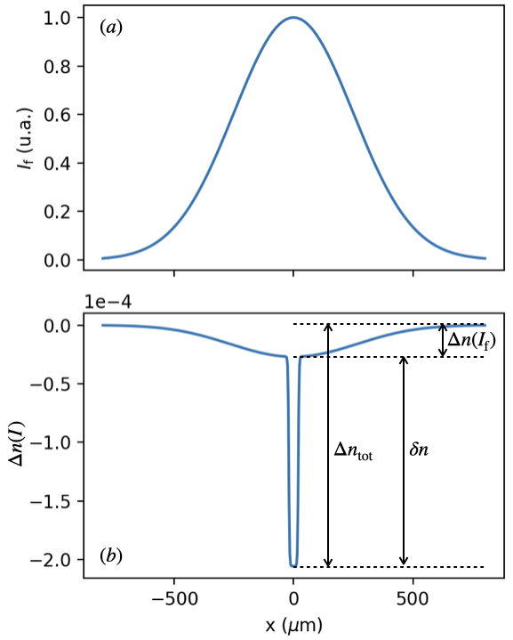
Figure 1: (a) Gaussian initial condition for the fluid beam, (b) effective index variation for the fluid beam, when it modifies itself the refractive index of the material through the photorefractive effect.

Figure 1(a) illustrates the input Gaussian beam, corresponding to the initial intensity profile for the fluid of light. The latter propagates in a medium in which we impose a local index variation $\Delta n(I_{\rm ob})=\delta n=-1.5\times 10^{-4}$. Figure 1(b) represents the total index variation, $\Delta n_{\rm tot}=\delta n+\Delta n(I_{\rm f})$, reflecting the fact that the fluid of light also contributes, nonlinearly, to the refractive index variation. As a consequence, the maximum variation of the total index of refraction is greater than $\delta n$, but in the example, this does not influence the fluid of light. However, a problem appears when the intensity of the obstacle beam makes the nonlinear refractive index variation saturate, which is commonly the case in this kind of experiments. Indeed, in this case, the nonlinear contribution imposed by the fluid itself induces an effective refractive index, $\Delta n_{\rm eff}$, lower than the maximum refractive index, $\Delta n_{\rm max}$, fixed by the obstacle. In order to evaluate the effective refractive index variation felt by the fluid of light, we develop an extension of the usual formula for the nonlinear index variation in a photorefractive crystal of SBN:61 denz2003 . We consider that the effective $\Delta n_{\rm eff}$ experienced by the fluid can be written as

$$\Delta n_{\rm eff}=\Delta n(I_{\rm f}+I_{\rm ob})-\Delta n(I_{\rm f}).$$ (5)

When assuming that the obstacle beam makes the nonlinear index saturate: $\Delta n(I_{\rm ob})=\Delta n_{\rm max}$, the previous equation reads

$$\Delta n_{\rm eff} = \Delta n_{\rm max}-\Delta n(I_{\rm f})$$ (6)

$$= \Delta n_{\rm max}-\Delta n_{\rm max}\frac{\tilde{I}_{\rm f}}{1+\tilde{I}_{\rm f}}$$

$$= \Delta n_{\rm max}\frac{1}{1+\tilde{I}_{\rm f}}.$$

It is then obvious that the effective refractive index seen by the fluid of light decreases as its intensity increases.

If we take the complete expression of eq. (5), then we need to plot a map of $\Delta n_{\rm eff}$ depending on $I_{\rm f}$ as well as on $I_{\rm ob}$. To do so, one can develop the expression of $\Delta n_{\rm eff}$ such as

$$\Delta n_{\rm eff}=\Delta n_{\rm max}\left[\frac{I_{\rm ob}/I_{\rm sat}}{1+\frac{2I_{\rm f}}{I_{\rm sat}}+\frac{I_{\rm ob}}{I_{\rm sat}}+\frac{\left(I_{\rm f}+I_{\rm ob}\right)I_{\rm f}}{I_{\rm sat}^{2}}}\right],$$ (7)

whose absolute value is plotted as a parametric plot in fig. 2. In this figure, we represent a contour plot whose different colors correspond to different values of $|\Delta n_{\rm eff}|$, with $I_{\rm ob}$ on the vertical axis and $I_{\rm f}$ on the horizontal axis. The white lines correspond to iso-index lines, and the orange dashed horizontal line corresponds to a typical $I_{\rm sat}$ of 400 mW/cm².

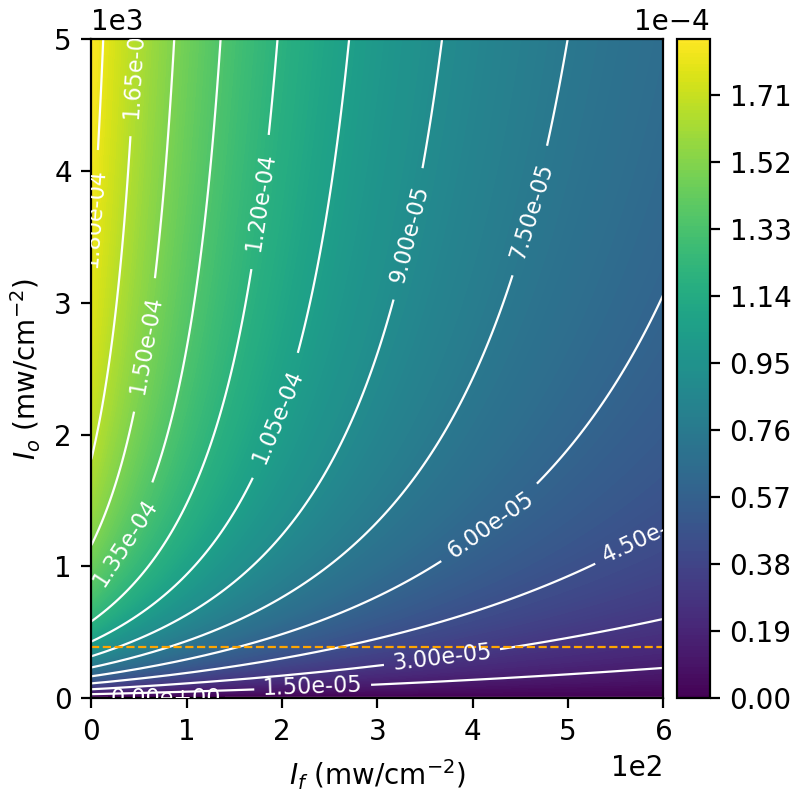
Figure 2: Cartography of the absolute value of the effective nonlinear index variation experienced by the fluid as a function of the fluid intensity on the horizontal axis, and the obstacle intensity on the vertical axis. The saturation intensity is denoted by the orange dashed horizontal line. The white lines correspond to iso-index lines.

Inspecting the limits of this expression, we can verify that we have the right intuition:

• if $I_{\rm ob}\gg I_{\rm sat}\gg I_{\rm f}$, then $\Delta n_{\rm eff}\rightarrow\Delta n_{\rm max}$, which is expected, as in this case, the obstacle beam completely makes the nonlinear index saturate. This corresponds to the upper left corner of the figure.

• if $I_{\rm ob}\ll I_{\rm f}$ and $I_{\rm f}\gg I_{\rm sat}$, then $\Delta n_{\rm eff}\rightarrow 0$. This is also expected as in this condition, the effect of the obstacle is overshadowed by the fluid, and if the fluid saturates the medium, the system goes back to linear. This corresponds to the lower right corner of the figure.

In the intermediate cases, it becomes obvious that the fluid beam almost never sees the maximum value of the nonlinear index variation. However, one can manage to optimise this value, and, more important, to keep it constant while varying $I_{\rm ob}$ and $I_{\rm f}$, following the white lines of fig. 2. This is what is done in the experiments presented in the main paper.

II Bogoliubov relation dispersion for a saturable nonlinearity

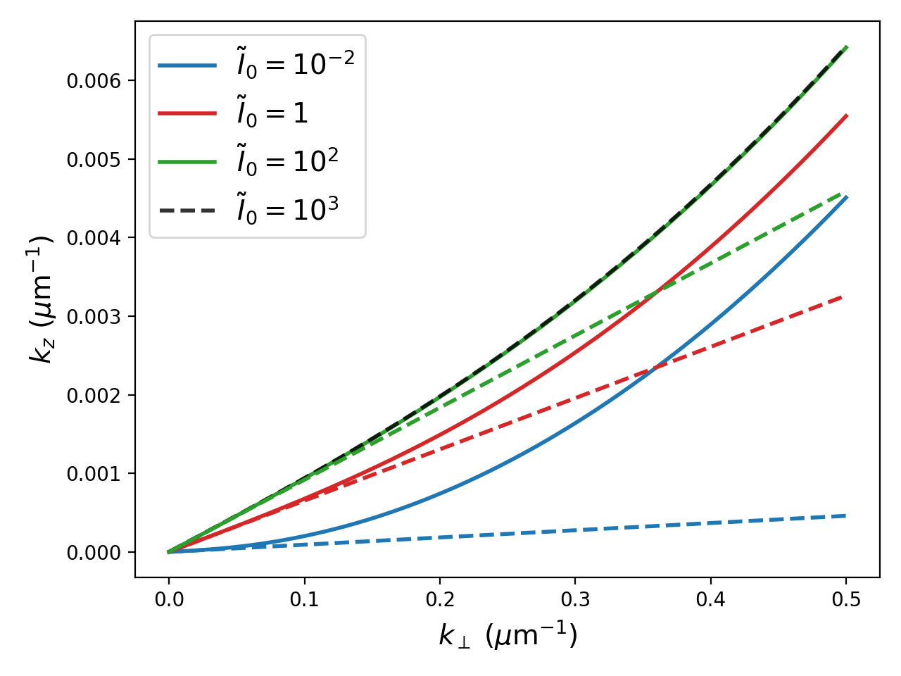
Figure 3: Dispersion relation of the elementary excitations on top of a homogeneous 2D fluid of light at rest. Blue, red and green solid lines, as well as the dotted-black line correspond to the dispersion relation (16) for different values of $\tilde{I}_{0}$. The dashed lines correspond to the $k_{\perp}\ll 1/\xi$ sonic regime, dominated by the nonlinearity. The slope of the straight lines directly provides the Bogoliubov sound velocity. In the deep saturation regime, the Bogoliubov dispersion relation is independent of the value of $\tilde{I}_{0}$, as the superposition of the green and black-dotted curves reveals.

In this section, we adapt Bogoliubov’s theory of linearised fluctuations to get the dispersion relation of the small modulations of the fluid of light in the nonlinear photorefractive crystal, in the simplest configuration where the fluid is uniform and at rest in the transverse plane. To do so, we start from the following nonlinear Schrödinger equation for the slowly varying wavefunction of the fluid:

$$i\partial_{z}\psi=-\frac{1}{2kn_{\rm e}}\nabla^{2}\psi-k\Delta n(I)\psi$$ (8)

where $\Delta n(I)=\Delta n_{\rm max}\frac{\tilde{I}}{1+\tilde{I}}$, with $\tilde{I}=I/I_{\rm sat}$ and $I=|\psi|^{2}$. Using the Madelung transformation $\psi(\mathbf{r})=\sqrt{I(\mathbf{r})}e^{iS(\mathbf{r})}$, it comes

$$\partial_{z}I+\frac{1}{kn_{\rm e}}\mathbf{\nabla}(I\mathbf{\nabla}S)=0,$$ (9)

$$\partial_{z}S=\frac{1}{2kn_{\rm e}}\frac{\nabla^{2}\sqrt{I}}{\sqrt{I}}-\frac{1}{2kn_{\rm e}}\left(\mathbf{\nabla}S\right)^{2}+k\Delta n(I),$$ (10)

Considering small perturbations on top of the homogeneous fluid at rest:

$$I = I_{0}+\delta I,$$ (11)

$$S = k\Delta n(I_{0})z+\delta S,$$ (12)

leads to the following equations for the perturbations:

$$\partial_{z}\delta I = -\frac{1}{kn_{\rm e}}I_{0}\nabla^{2}\delta S,$$ (13)

$$\partial_{z}\delta S = \frac{1}{4kn_{\rm e}}\frac{1}{I_{0}}\nabla^{2}\delta I+k\Delta n_{\rm max}\frac{\delta\tilde{I}}{(1+I_{0}^{2})}.$$ (14)

Deriving the latter with respect to $z$ and combining it with the former, we eventually get, for the phase fluctuations,

$$\partial_{z}^{2}\delta S=-\frac{1}{4k^{2}n_{\rm e}^{2}}\nabla^{4}\delta S+\frac{\Delta n(I_{0})}{n_{\rm e}}\nabla^{2}\delta S.$$ (15)

To get the dispersion relation of the fluctuations on top of the fluid, we search for the solution of eq. (16) in the plane-wave form $S\propto\exp{\left[i\left(\mathbf{k}_{\perp}\cdot\mathbf{r}+k_{z}z\right)\right]}$, which leads to the following Bogoliubov-type dispersion relation:

$$k_{z}=\sqrt{\frac{k_{\perp}^{2}}{2kn_{\rm e}}\left(\frac{k_{\perp}^{2}}{2kn_{\rm e}}+2k\Delta n(I_{0})\right)}.$$ (16)

From this equation, one extract the healing length and the sound velocity, which are

$$\xi = \frac{1}{\sqrt{k^{2}n_{\rm e}|\Delta n(I_{0})|}},$$ (17)

$$c_{\rm s} = \sqrt{\frac{|\Delta n(I_{0})|}{n_{\rm e}}}.$$ (18)

Figure 3 displays the Bogoliubov dispersion relation as a function of the transverse wavenumber $k_{\perp}$ for different values of $\tilde{I}_{0}$ and typical experimental parameters. Obviously, when $\tilde{I}_{0}\ll 1$, the nonlinear contribution is negligible, and the sound velocity, corresponding to the slope of the linear part of the dispersion relation at low $k_{\perp}$ tends to $0$. On the other hand, when $\tilde{I}_{0}\gg 1$, the saturation manifests in the fact that the shape of the dispersion relation does not change anymore when increasing $\tilde{I}_{0}$. However, the typical linear and parabolic trends of the dispersion for respectively $k_{\perp}\ll 1/\xi$ and $k_{\perp}\gg 1/\xi$ remain. Nevertheless, it is important in the experiment that the hydrodynamical parameters (i.e., $c_{\rm s}$, $\xi$) still depend on the fluid density, so we take care of never exceeding $\tilde{I}_{0}=1$.

References

[1]
O. Boughdad et al.
Anisotropic nonlinear refractive index measurement of a
photorefractive crystal via spatial self-phase modulation.
Opt. Express, 27(21):30360, 2019.
[2]
C. Denz et al.
Transverse-Pattern Formation in Photorefractive Optics.
Springer-Verlag, Berlin, 2003.