Critical behavior of charged AdS black holes surrounded by quintessence
via an alternative phase space

Abstract

Considering the variable cosmological constant in the extended phase space has a significant background in the black hole physics. It was shown that the thermodynamic behavior of charged AdS black hole surrounded by the quintessence in the extended phase space is similar to the van der Waals fluid. In this paper, we indicate that such a black hole admits the same criticality and van der Waals like behavior in the non-extended phase space. In other words, we keep the cosmological constant as a fixed parameter, and instead, we consider the normalization factor as a thermodynamic variable. We show that there is a first-order small/large black hole phase transition which is analogous to the liquid/gas phase transition in fluids. We introduce a new picture of the equation of state and then we calculate the corresponding critical quantities. Moreover, we obtain the critical exponents and show that they are the same values as the van der Waals system. Finally, we study the photon sphere and the shadow observed by a distant observer and investigate how the shadow radius may be affected by the variation of black hole parameters. We also investigate the relations between shadow radius and phase transitions and calculate the critical shadow radius where the black hole undergoes a second-order phase transition.

I Introduction

Undoubtedly, the black hole (BH) is one of the most fascinating and mysterious subjects in the world of physics as well as mathematics. BH was one of the interesting predictions of general relativity which is confirmed by observational data LIGO . The observational evidence of massive objects and detection of the gravitational waves open a new window in modern mathematical physics and data analysis. On the other hand, the discovery of a profound connection between the laws of BH mechanics with the corresponding laws of ordinary thermodynamic systems has been one of the remarkable achievements of theoretical physics Bardeen ; Hawking . In other words, the consideration of a BH as a thermodynamic system with a physical temperature and an entropy opened up new avenues in studying their microscopic structure.

In the past two decades, the study of BH thermodynamics in an anti-de Sitter (AdS) space attracted significant attention. Strictly speaking, the investigation of thermodynamic properties of black holes in such a spacetime provides a deep insight to understand the quantum nature of gravity Maldacena ; Witten . In particular, the phase transition of AdS black holes has gained a lot of attention due to the AdS/CFT correspondence in recent years. The pioneering work in this regard was realized by Hawking and Page who proved the existence of a certain phase transition (so called Hawking-Page) between thermal radiation and Schwarzschild-AdS BH Hawking1 . Afterward, our understanding of phase transition has been extended by studying in more complicated backgrounds Cvetic1 ; Cvetic2 . Among conducted efforts, thermodynamics of charged black holes in the background of an asymptotically AdS spacetime is of particular interest, due to a complete analogy between them and the van der Waals liquid-gas system. Such an analogy will be more precise by considering the cosmological constant as a dynamical pressure and its conjugate quantity as a thermodynamic volume in the extended phase space Kubiznak1 .

It is worthwhile to mention that the conducted investigations in this regard are based on the first law and Smarr relation by comparing BH mechanics with ordinary thermodynamic systems not CFT point of view. Despite the interesting achievements of AdS/CFT correspondence such as describing the Hawking radiation mechanism and dual interpretation of Hawking-Page phase transition and so on with fixed $\Lambda$, this method is not yet able to provide a suitable picture in the extended thermodynamics. In the context of AdS/CFT correspondence, the cosmological constant is set by $N$, related to the number of coincident branes ($M$ branes or $D$ branes) on the gravity side. On the field theory side, $N$ is typically the rank of a gauge group of the theory, and as such, it also determines the maximum number of available degrees of freedom. The thermodynamic volume in the bulk gravity theory corresponds to the chemical potential in the boundary field theory which is the conjugate variable of the number of colors Kubiznak3 ; Johnson . Variation of the pressure of the bulk, or equivalently variation of the AdS radius ($l$) leads to variation of the boundary quantities: i) the number of colors $N$. ii) the volume of the space on which the field theory is formulated (since $V\propto l^{d-2}$). iii) the CFT charge $Q$ which is related to the bulk charge $Q_{b}$ according to $Q=lQ_{b}$. So, considering the cosmological constant as a new thermodynamical parameter may give the phase diagram an extra dimension. An alternative interpretation is suggested in Karch , where the variation of the pressure in the bulk theory corresponds to vary the volume of the boundary field theory. In this approach, the number of colors is kept fixed, which requires the variation of Newton’s constant to compensate the variation of the volume of the boundary field theory. This shows that one cannot employ such an approach (AdS/CFT correspondence) to investigate the extended thermodynamics of black holes.

Considering the defined thermodynamic pressure and volume, one can study thermodynamics of black holes in a new framework, sometimes referred to as BH Chemistry Mann . This change of perspective has led to a different concept of known processes and the discovery of a broad range of new phenomena associated with black holes such as van der Waals behavior Kubiznak1 ; Kubiznak2 , solid/liquid phase transitions Altamirano , triple points WWei , reentrant phase transitions Kubiznak4 and heat engines Johnson . Also, using BH volume, one can study the BH adiabatic compressibility which has attracted attention in connection with BH stability Dolan1 . This new perspective has also been successful in describing the thermodynamic structure of black holes in other gravitational theories such as Lovelock gravity Dolan2 , nonlinear electrodynamics Hendi , Einstein-Yang-Mills gravity Zhang1 , black holes with scalar hair Hristov1 , dyonic black holes Dutta , f(R) gravity Chen , STU black holes Caceres , quasi topological gravity Hennigar1 , conformal gravity Zhao1 Poincare gauge gravity ZLiu , Lifshitz gravity Brenna ; Jafarzade ; Zeng and massive gravity Hendi1 .

Since the thermodynamic behavior of BH is highly affected by the variation of electric charge, an alternative approach for investigating van der Waals like phase transition is proposed Chamblin1 ; Chamblin2 by considering the electric charge as a thermodynamic variable and fixing the cosmological constant. In this regard, a phase transition between the large and small black holes in the $Q-\Phi$ plane is seen. In addition, it is shown that Dehyadegari such a suggestion is mathematically problematic and physically unconventional and it is logical to consider the square of the electric charge, $Q^{2}$, as a thermodynamic variable. In Ref. Dehyadegari , the van der Waals like behavior of charged AdS BH in $Q^{2}-\Psi$ plane with a fixed cosmological constant is studied. It is also obtained the critical exponents which were exactly coincident with those obtained for van der Waals liquid. As a keynote, we should emphasize that unlike the van der Waals liquid the mentioned phase transition occurred for temperature higher than critical temperature ($T>T_{c}$) in $Q^{2}-\Psi$ plane. However, $Q^{2}-\Psi$ criticality has been investigated in alternative theories of gravity Yazdikarimi .

Alternative theories of gravity are proposed to overcome different shortcomings of Einstein’s general relativity. In recent years, modern observational evidence has shown that the universe is expanding with acceleration, demanding the existence of dark energy Bachall ; Sahni . Among the various dark energy candidates, consideration of the cosmological constant or the quintessence is more common. The quintessence is proposed as the canonical scalar field with state parameter $-1<\omega<1$. However, in order to explain the late-time cosmic acceleration, one has to restrict such a parameter to $-1<\omega<-\frac{1}{3}$. The cases of $\omega=\frac{1}{3}$ and $\omega=0$ are, respectively, representing the radiation and dust around the black hole, while the quintessential dark energy likes cosmological constant for $\omega\longrightarrow-1$. As the first attempt, Kiselev obtained the solutions of Einstein’s field equations for the quintessence matter around a charged (an uncharged) BH Kiselev . These solutions are described in terms of the state parameter $\omega$ and the normalization factor $a$. The normalization factor indicates the intensity of the quintessence field and the state parameter refers to its nature and behavior. The rotating generalization of Kiselev solutions and their AdS modifications have been reported in Refs. Ghosh ; Oteev ; Toshmatov ; Xu . In addition to the exact Kiselev solutions and their generalizations, considerable efforts were conducted in context of thermodynamic and phase transition of such black holes Majeed ; Wang2 . The obtained results showed that variation of the quintessence field affects the thermodynamic behavior of quintessential black holes and consequently, it can lead to interesting critical behavior. Such a criticality is studied in $Q^{2}-\Psi$ and $P-V$ planes, as common methods. It will be interesting to probe the van der Waals like phase transition and critical behavior by treating the normalization factor as a thermodynamic variable and keeping both the cosmological constant and electric charge as fixed parameters. To achieve this goal, we would like to investigate the critical behavior of Reissner-Nordström-AdS (RN-AdS) black holes surrounded by quintessence via this alternative viewpoint.

The organization of this paper is as follows. In the next section, we would like to give a brief review of RN-AdS black holes surrounded by quintessence and their criticality via the common methods. In Sec. III, we study the critical behavior of the corresponding BH solution using the alternative phase space. We will calculate the critical exponents and compare the obtained results with those obtained for van der Waals fluid. Sec. IV is devoted to exploring the photon orbits near the black hole and formation of shadow. In Sec. IV.1, we investigate the connection between BH shadow and phase transition. Finally, we finish the paper with concluding remarks.

II Thermodynamics of charged AdS BH surrounded by quintessence: A brief review

In this section, we first introduce the thermodynamics charged AdS BH surrounded by quintessence by reviewing Refs. Li ; Liu ; Hong ; Guo . The line element of such a BH is expressed as

$$ds^{2}=-f(r)dt^{2}+\frac{1}{f(r)}dr^{2}+r^{2}d\theta^{2}+r^{2}sin^{2}\theta\;d\phi^{2},$$ (1)

where

$$f(r)=1-\frac{2M}{r}+\frac{Q^{2}}{r^{2}}-\frac{a}{r^{3\omega+1}}+\frac{r^{2}}{l^{2}},$$ (2)

where $M$ and $Q$ are the mass and electric charge of the black hole, respectively and $\ell=\sqrt{-\frac{3}{\Lambda}}$ is the AdS radius which is related to the cosmological constant. The state parameter $\omega$ describes the equation of state $p=\omega\rho$ where $p$ and $\rho$ are the pressure and energy density of the quintessence, respectively. The normalization factor $a$ is related to the density of quintessence $\rho$ as

$$\rho=-\frac{a}{2}\frac{3\omega}{r^{3(1+\omega)}},$$ (3)

with $[length]^{-2}$ dimensions. Solving the equation $(f(r=r_{+})=0)$, one can obtain the total mass of the BH ($M$) as

$$M=\frac{r_{+}}{2}+\frac{Q^{2}}{2r_{+}}+\frac{r_{+}^{3}}{2l^{2}}-\frac{a}{2}r_{+}^{-3\omega}.$$ (4)

In addition, one can use the Hawking and Bekenstein area law to obtain the entropy as

$$S=\frac{A}{4}=\pi r_{+}^{2}.$$ (5)

Working in the extended phase space, the cosmological constant and thermodynamic pressure are related to each other with the following relation

$$P=-\frac{\Lambda}{8\pi}=\frac{3}{8\pi l^{2}},$$ (6)

where the variability of the cosmological constant is associated to the dynamical vacuum energy.

It it easy to rewrite Eq. (4) in terms of pressure and entropy as

$$M(S,Q,P,a)=\frac{1}{6\sqrt{\pi S}}\left(3\pi Q^{2}+3S+8PS^{2}-3a\pi^{\frac{3\omega+1}{2}}S^{\frac{1-3\omega}{2}}\right).$$ (7)

It is obvious that the total mass of BH plays the role of enthalpy instead of internal energy in the extended phase space. Therefore, regarding the enthalpy representation of the first law of BH thermodynamics, the intensive parameters conjugate to $S$, $Q$, $P$ and $a$ are, respectively, calculated as

$$T\equiv\left(\frac{\partial M}{\partial S}\right)_{P,Q,a} = \frac{1}{4\pi r_{+}}\left(1-\frac{Q^{2}}{r_{+}^{2}}+8\pi Pr_{+}^{2}+3\omega ar_{+}^{-3\omega-1}\right),$$ (8)

$$\Phi\equiv\left(\frac{\partial M}{\partial Q}\right)_{S,P,a} = \frac{Q}{r_{+}},$$ (9)

$$V\equiv\left(\frac{\partial M}{\partial P}\right)_{S,Q,a} = \frac{4}{3}\pi r_{+}^{3},$$ (10)

$$y\equiv\left(\frac{\partial M}{\partial a}\right)_{S,Q,P} = -\frac{1}{2}r_{+}^{-3\omega},$$ (11)

where $T$, $\Phi$ and $V$ are the temperature, electric potential and thermodynamic volume, respectively and $y$ is the quantity conjugate to the dimensionful factor $a$. Considering the dimensional analysis, we can obtain the following Smarr relation

$$M=2TS+\Phi Q-2VP+(1+3\omega)ya,$$ (12)

where confirms that we have to regard $a$ as a thermodynamic quantity. Now, it is straightforward to find that the first law of the BH is obtained as

$$dM=TdS+\Phi dQ+VdP+yda.$$ (13)

II.1 $P-V$ criticality and van der Waals phase transition: Usual method

In this section, we briefly review the critical behavior of such black holes in the usual way. Considering the temperature relation, Eq. (8) with the definition of pressure, Eq. (6), one can easily derive the equation of state of the BH as

$$P=\frac{T}{2r_{+}}-\frac{1}{8\pi r_{+}^{2}}+\frac{Q^{2}}{8\pi r_{+}^{4}}-\frac{3a\omega}{8\pi r_{+}^{3(1+\omega)}}.$$ (14)

Since the event horizon radius $r_{+}$ is associated with the van der Waals fluid specific volume ($\upsilon$) Kubiznak1 ; Kubiznak2 ; Li as $\upsilon={2\ell_{\rm{P}}^{{2}}{r_{+}}}$ ( $\ell_{\rm{P}}$ is the Planck length that we set $\ell_{\rm{P}}=1$ since we work in the geometric units), Eq. (14) can be rewritten as

$$P=\frac{T}{\upsilon}-\frac{1}{2\pi\upsilon^{2}}+\frac{2Q^{2}}{\pi\upsilon^{4}}-\frac{8^{\omega}\times 3a\omega}{\pi\upsilon^{3(1+\omega)}}.$$ (15)

The corresponding $P-V$ and $T-V$ diagrams are depicted in Fig. 1. Evidently, the behavior is reminiscent of the van der Waals fluid which confirms the first-order small-large BH transition for temperatures smaller than the critical temperature. The critical point can be extracted from

$$\frac{\partial p}{\partial\upsilon}\bigg{|}_{\upsilon=\upsilon_{c},T=T_{c}}=0~{}~{}~{}\&~{}~{}~{}\frac{\partial^{2}p}{\partial\upsilon^{2}}\bigg{|}_{\upsilon=\upsilon_{c},T=T_{c}}=0.$$ (16)

which results into the following equation for calculating critical volume

$$\upsilon_{c}^{3\omega+1}-24Q^{2}\upsilon_{c}^{3\omega-1}+8^{\omega}\times 9a\omega(2+5\omega+3\omega^{2})=0.$$ (17)

The critical temperature and pressure is calculated as

$$T_{c} = \frac{1}{\pi\upsilon_{c}}-\frac{8Q^{2}}{\pi\upsilon_{c}^{3}}+\frac{8^{\omega}\times 9a\omega(\omega+1)}{\pi\upsilon_{c}^{3\omega+2}},$$

$$P_{c} = \frac{1}{2\pi\upsilon_{c}^{2}}-\frac{6Q^{2}}{\pi\upsilon_{c}^{4}}+\frac{8^{\omega}\times 9a\omega(2+3\omega)}{\pi\upsilon_{c}^{3\omega+3}}.$$ (18)

Equation (17) can be analytically solved for $\omega=-\frac{2}{3}$, resulting into the following critical quantities

$$\upsilon_{c}=2\sqrt{6}Q;~{}~{}~{}~{}T_{c}=\frac{\sqrt{6}}{18\pi Q}-\frac{a}{2\pi};~{}~{}~{}~{}P_{c}=\frac{1}{96\pi Q^{2}}.$$ (19)

It is worthwhile to mention that the critical volume and pressure are exactly the same as those presented for RN-AdS BH Kubiznak1 , and only the critical temperature is affected by quintessence dark energy. For $a=0$, all these critical quantities reduce to those of the RN-AdS black hole.

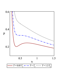
(a)

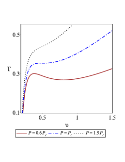
(b)

Figure 1: The van der Waals like phase diagrams for $Q=0.1$, $\omega=-\frac{2}{3}$ and $a=0.5$.

III Critical Behavior of the charged AdS BH surrounded by quintessence: An alternative approach

Kubiznak and Mann in Ref. Kubiznak1 showed that charged AdS black holes have a critical behavior similar to van der Waals fluid in the extended phase space. Li also employed such an idea for investigating the critical behavior of the charged AdS BH surrounded by quintessence Li . Although the idea of considering the variable cosmological constant has attracted a lot of attention in BH thermodynamics, it was shown that by keeping the cosmological constant as a fixed parameter and instead considering the square of electric charge as a thermodynamic variable, one can observe such a critical behavior in $Q^{2}-\Psi$ plane Dehyadegari . The study of phase transition via this alternative approach was made for the charged AdS BH in the presence of quintessence field in Ref. Chabab . Now, we are interested in studying the critical behavior of charged AdS black holes surrounded by quintessence via a new approach by considering both the cosmological constant (Eq. 6) and electric charge as fixed external parameters and allow the normalization factor to vary. Here, we investigate critical behavior of the system for two different cases to find a proper alternative approach.

III.1 Critical behavior of the BH via approach I

In this subsection, we consider the normalization factor $a$ as a thermodynamic variable and study the critical behavior of the system under its variation. We start by writing the equation of state in the form $a(T,y)$ by using Eq. (8). Inserting Eq. (11) into the relation of temperature, the equation of state is obtained as

$$a(T,y)=\frac{4\pi T}{3\omega(-2y)^{\frac{3\omega+2}{3\omega}}}+\frac{Q^{2}}{3\omega(-2y)^{\frac{3\omega-1}{3\omega}}}-\frac{1}{3\omega(-2y)^{\frac{3\omega+1}{3\omega}}}-\frac{1}{\omega l^{2}(-2y)^{\frac{3\omega+3}{3\omega}}}.$$ (20)

In order to investigate the critical behavior of the system and compare with the van der Waals fluid, we should plot isotherm diagrams. The corresponding $a-y$ diagram is illustrated in Figs. 2(a) and 2(d). The diagrams show that, for constant $Q$ and $l$, there is an inflection point which may be interpreted as the critical point where two phases of small and large black holes are in equilibrium. Using the equation of state (20) and the concept of the inflection point, the critical point can be characterized by

$$\frac{\partial a}{\partial y}\bigg{|}_{y=y_{c},T=T_{c}}=0~{}~{}~{}\&~{}~{}~{}\frac{\partial^{2}a}{\partial y^{2}}\bigg{|}_{y=y_{c},T=T_{c}}=0,$$ (21)

which leads to

$$y_{c} = -\frac{1}{2}\left(\frac{\sqrt{2l}}{6}\sqrt{\frac{l(1+3\omega)+\sqrt{108Q^{2}(1+\omega)(1-3\omega)+l^{2}(1+3\omega)^{2}}}{1+\omega}}\right)^{-3\omega},$$

$$T_{c} = \frac{Q^{2}l^{2}(1-3\omega)(-2y_{c})^{\frac{1}{\omega}}+l^{2}(1+3\omega)(-2y_{c})^{\frac{1}{3\omega}}+9(1+\omega)(-2y_{c})^{-\frac{1}{3\omega}}}{4\pi l^{2}(2+3\omega)},$$

$$a_{c} = \frac{3+3Q^{2}l^{2}(-2y_{c})^{\frac{4}{3\omega}}-l^{2}(-2y_{c})^{\frac{2}{3\omega}}}{\omega l^{2}(3\omega+2)(-2y_{c})^{\frac{\omega+1}{\omega}}}.$$ (22)

Studying the heat capacity, one can confirm the criticality behavior mentioned above via the method of reported in Refs. HendiA ; HendiB . After some manipulations, we find

$$C=\frac{2\pi\left(l^{2}+3(-2y)^{-\frac{2}{3\omega}}-Q^{2}l^{2}(-2y)^{\frac{2}{3\omega}}+3a\omega l^{2}(-2y)^{\frac{1+3\omega}{3\omega}}\right)}{3-l^{2}(-2y)^{\frac{2}{3\omega}}+3Q^{2}l^{2}(-2y)^{\frac{4}{3\omega}}-3(2+3\omega)a\omega l^{2}(-2y)^{\frac{3+3\omega}{3\omega}}}.$$ (23)

Solving denominator of the heat capacity with respect to $a$, a new relation for normalization factor $(a_{new})$ is obtained which is different from what was obtained in Eq. (20). $a_{new}$ is obtained as follows

$$a_{new}=\frac{3+3Q^{2}l^{2}(-2y)^{\frac{4}{3\omega}}-l^{2}(-2y)^{\frac{2}{3\omega}}}{\omega l^{2}(3\omega+2)(-2y)^{\frac{\omega+1}{\omega}}}.$$ (24)

Evidently, the above relation diverges at $\omega=-\frac{2}{3}$ . This new relation for normalization factor $a$ has an extremum which exactly coincides with the inflection point of $a-y$ diagram (see dashed lines in Figs. 2(a) and 2(d)). In other words, its extremum is the same critical normalization factor and its proportional $y$ (in which $a_{new}$ is maximum) is $y_{c}$. By deriving the new normalization factor with respect to $y$, one can obtain $y_{max}$ as

$$y_{max} = -\frac{1}{2}\left(\frac{\sqrt{2l}}{6}\sqrt{\frac{l(1+3\omega)+\sqrt{108Q^{2}(1+\omega)(1-3\omega)+l^{2}(1+3\omega)^{2}}}{1+\omega}}\right)^{-3\omega},$$ (25)

which is the same $y_{c}$ in Eq. (22). It is evident that by inserting Eq. (25) into Eq. (24), one can reach $a_{c}$ (compare $a_{new}$ to $a_{c}$ in Eq. (22)). As we see from Fig. 2(a), for $\omega>-\frac{2}{3}$, the new normalization factor has a maximum which matches to the inflection point of $a-y$ diagram. Whereas an opposite behavior can be observed for $\omega<-\frac{2}{3}$ (see Fig. 2(d)). The phase structure of a thermodynamic system can also be characterized by the Gibbs free energy, $G=M-ST$. The behavior of the Gibbs free energy in term of $T$ is depicted in Figs. 2(b) and 2(e). The existence of swallow-tail shape in $G-T$ diagram indicates that the system has a first order phase transition from small BH to large black hole. For $\omega>-\frac{2}{3}$, system undergoes a first order phase transition for $a<a_{c}$ (see Fig. 2(b)) and $T>T_{c}$ (see Fig. 2(a)). Whereas for $\omega<-\frac{2}{3}$, such a phase transition is observed for $a>a_{c}$ and $T<T_{c}$ (see Figs. 2(d) and 2(e)). The coexistence line of two phases of small and large black holes, along which these two phases are in equilibrium, is obtained from Maxwell’s equal area law. Figures 2(c) and 2(f) displays the coexistence line of small-large BH phase transition. The critical point is highlighted by a small circle at the end of the coexistence line.

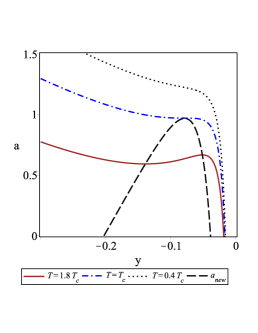
(a) $Q=0.1$ and $\omega=-0.5$

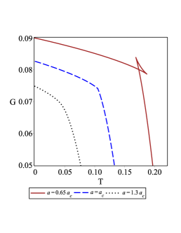
(b) $Q=0.1$ and $\omega=-0.5$

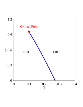
(c) $Q=0.1$ and $\omega=-0.5$

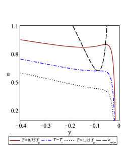
(d) $Q=0.2$ and $\omega=-0.8$

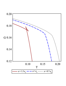
(e) $Q=0.2$ and $\omega=-0.8$

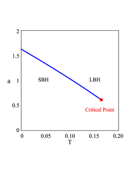
(f) $Q=0.2$ and $\omega=-0.8$

Figure 2: Left panels: The behavior of isothermal $a-y$. Middle panels: the Gibbs free energy diagram $G-T$. Right panels: Coexistence curve of small-large BH phase transition in the $a-T$ plane.

Critical exponents

Critical exponents describe the behavior of physical quantities near the critical point. For fixed dimensionality and range of interactions, the critical exponents are independent of the details of a physical system, and therefore, one may regard them quasi-universal. Now, we aim to calculate the critical exponents in this new approach. To do so, we first introduce the following useful relations

$$C_{y}=\mid t\mid^{-\alpha},~{}~{}~{}\eta=\mid t\mid^{\lambda},~{}~{}~{}\kappa_{T}=\mid t\mid^{-\gamma},~{}~{}~{}\mid a-a_{c}\mid=\mid y-y_{c}\mid^{\delta}.$$ (26)

where the critical exponents $\alpha$ , $\lambda$, $\gamma$ and $\delta$ describe the behavior of specific heat $C_{y}$, the order parameter $\eta$, the isothermal compressibility $\kappa_{T}$ and behavior on the critical isotherm $T=T_{c}$, respectively. To find the critical exponent, we define the below dimensionless quantities

$$\xi=\frac{a}{a_{c}},~{}~{}~{}\zeta=\frac{y}{y_{c}},~{}~{}~{}\tau=\frac{T}{T_{c}}.$$ (27)

Since the critical exponents are studied near the critical point, we can write the reduced variables in the following form

$$\zeta=1+\nu,~{}~{}~{}\tau=1+t.$$ (28)

First, we rewrite the entropy in terms of $T$ and $y$ as,

$$S(T,y)=\pi(-2y)^{\frac{2}{3\omega}},$$ (29)

which is independent of temperature. So, we find that

$$C_{y}=T\frac{\partial S}{\partial T}\bigg{|}_{y}=0,$$ (30)

and hence $\alpha=0$. By using Eq. (28), one can expand Eq. (20) near the critical point as

$$\xi=\mathcal{A}+A_{1}t+\mathcal{A}_{1}\nu t+\mathcal{A}_{2}\nu+\mathcal{A}_{3}\nu^{2}+\mathcal{A}_{4}\nu^{3}+O(t\nu^{2},\nu^{4}),$$ (31)

where

$$\mathcal{A}_{1} = -\frac{1}{3\omega}A_{1}(2+3\omega),$$

$$\mathcal{A}_{2} = -\frac{1}{3\omega}\left(3\mathcal{A}\omega+2A_{1}-A_{2}+A_{3}+3A_{4}\right),$$

$$\mathcal{A}_{3} = \frac{1}{18\omega^{2}}\left(9\omega(2A_{1}-A_{2}+A_{3}+3A_{4})+3A_{1}+8A_{4}+\mathcal{A}+18\mathcal{A}\omega^{2}\right),$$

$$\mathcal{A}_{4} = -\frac{1}{162\omega^{3}}\left(99\omega^{2}(2A_{1}-A_{2}+A_{3}+3A_{4})+18\omega(\mathcal{A}+3A_{1}+8A_{4})+8A_{1}-A_{2}+A_{3}+27A_{4}+162\mathcal{A}\omega^{3}\right),$$ (32)

and

$$\mathcal{A} = A_{1}+A_{2}+A_{3}+A_{4},~{}~{}~{}A_{1}=\frac{4\pi T_{c}}{3\omega a_{c}(-2y_{c})^{\frac{3\omega+2}{3\omega}}},~{}~{}~{}A_{2}=\frac{Q^{2}}{3\omega a_{c}(-2y_{c})^{\frac{3\omega-1}{3\omega}}},$$

$$A_{3} = -\frac{1}{3\omega a_{c}(-2y_{c})^{\frac{3\omega+1}{3\omega}}},~{}~{}~{}A_{4}=-\frac{1}{\omega a_{c}l^{2}(-2y_{c})^{\frac{3\omega+3}{3\omega}}}.$$ (33)

$Q$	$\omega$	$y_{c}$	$T_{c}$	$a_{c}$	$\mathcal{A}$	$A_{1}$	$\mathcal{A}_{1}$	$\mathcal{A}_{2}$	$|\mathcal{A}_{3}|$	$\mathcal{A}_{4}$
$~{}0.1~{}$	$~{}-0.4~{}$	$~{}-0.12~{}$	$~{}0.17~{}$	$~{}0.52~{}$	$~{}0.99~{}$	$~{}-1.35~{}$	$~{}-0.9~{}$	$~{}<10^{-10}~{}$	$~{}<10^{-10}~{}$	$~{}0.46~{}$
$~{}0.1~{}$	$~{}-0.5~{}$	$~{}-0.07~{}$	$~{}0.09~{}$	$~{}0.96~{}$	$~{}1.0~{}$	$~{}0.45~{}$	$~{}-0.15~{}$	$~{}<10^{-10}~{}$	$~{}<10^{-10}~{}$	$~{}0.15~{}$
$~{}0.15~{}$	$~{}-0.6~{}$	$~{}-0.09~{}$	$~{}0.16~{}$	$~{}0.59~{}$	$~{}1.0~{}$	$~{}-1.57~{}$	$~{}-0.17~{}$	$~{}<10^{-9}~{}$	$~{}<10^{-10}~{}$	$~{}0.21~{}$
$~{}0.18~{}$	$~{}-0.7~{}$	$~{}-0.08~{}$	$~{}0.11~{}$	$~{}0.96~{}$	$~{}1.0~{}$	$~{}-0.7~{}$	$~{}0.03~{}$	$~{}<10^{-9}~{}$	$~{}<10^{-10}~{}$	$~{}0.09~{}$
$~{}0.2~{}$	$~{}-0.8~{}$	$~{}-0.08~{}$	$~{}0.16~{}$	$~{}0.61~{}$	$~{}0.99~{}$	$~{}-1.87~{}$	$~{}0.31~{}$	$~{}<10^{-9}~{}$	$~{}<10^{-9}~{}$	$~{}0.10~{}$
$~{}0.2~{}$	$~{}-0.9~{}$	$~{}-0.06~{}$	$~{}0.20~{}$	$~{}0.39~{}$	$~{}1.0~{}$	$~{}-3.98~{}$	$~{}1.03~{}$	$~{}<10^{-9}~{}$	$~{}<10^{-9}~{}$	$~{}0.11~{}$

Table 1: Numerical solution of the coefficients $\mathcal{A}_{i}$ for $l=1$.

Considering table 1, it is evident that the coefficients $\mathcal{A}_{2}$ and $\mathcal{A}_{3}$ can be ignorable. So, Eq. (31) reduces to

$$\xi=\mathcal{A}+A_{1}t+\mathcal{A}_{1}\nu t+\mathcal{A}_{4}\nu^{3},$$ (34)

Differentiating Eq. (34) with respect to $\nu$ for a fixed $t$, we get

$$da=a_{c}(\mathcal{A}_{1}t+3\mathcal{A}_{4}\nu^{2})d\nu,$$ (35)

Now, using the fact that the normalization factor remains constant during the phase transition and employing the Maxwell’s area law, we have the following two equations:

$$\xi = A_{1}t+\mathcal{A}_{1}\nu_{l}t+\mathcal{A}_{4}\nu_{l}^{3}=A_{1}t+\mathcal{A}_{1}\nu_{s}t+\mathcal{A}_{4}\nu_{s}^{3},$$

$$0 = \int_{\nu_{l}}^{\nu_{s}}\nu(\mathcal{A}_{1}t+3\mathcal{A}_{4}\nu^{2})d\nu,$$ (36)

where $\nu_{s}$ and $\nu_{l}$ denote the event horizon of small and large black holes, respectively. Equation (36) has a unique non-trivial solution given by

$$\nu_{s}=-\nu_{l}=\sqrt{-\frac{\mathcal{A}_{1}}{\mathcal{A}_{4}}t}.$$ (37)

According to the table 1, the argument under the square root function is always positive. From Eq. (37), one can find that

$$\eta=y_{c}(\nu_{l}-\nu_{s})=2y_{c}\nu_{l}=2\sqrt{-\frac{\mathcal{A}_{1}}{\mathcal{A}_{4}}t}~{}~{}\Longrightarrow~{}~{}\lambda=\frac{1}{2}.$$ (38)

Now, we can differentiate Eq. (34) to calculate the critical exponent $\gamma$ as

$$\kappa_{T}=-\frac{1}{y}\frac{\partial y}{\partial a}\bigg{|}_{T}\propto\frac{y_{c}}{\mathcal{A}_{1}a_{c}t}~{}~{}\Longrightarrow~{}~{}\gamma=1.$$ (39)

Finally, the shape of the critical isotherm $t=0$ is given by

$$\xi-\mathcal{A}=\mathcal{A}_{4}\nu^{3}~{}~{}\Longrightarrow~{}~{}\delta=3.$$ (40)

The obtained results show that the critical exponents in this new approach (with fixed $\Lambda$ and variable $a$) are the same as those obtained in Li (with $\Lambda$ variable and fixed $a$) and coincide with the van der Waals fluid system Kubiznak1 .

III.2 Critical behavior of the BH via approach II

One of the issues in previous section III.1 (considering the positive normalization factor as a thermodynamic variable) is that we could not interpret (or adapt) the positive $a$ and its negative definite conjugate $y=\left(\frac{\partial M}{\partial a}\right)_{P,Q,S}=-\frac{1}{2}r_{+}^{-3\omega}$ ($[y]=[length]^{-3\omega}$) with the known thermodynamical quantities. Besides, considering Fig. 1a with Fig. 2d, one has to apply a rotation of $\pi$ radian for an appropriate comparison.

Here, we define a new parameter depending on the normalization factor with $[length]^{-2}$ dimensions to adapt it (its conjugate) as an ad hoc pressure (volume). Here, we consider negative values of normalization factor (with negative $\omega$) to define a positive variable $\beta$ as

$$\beta=\frac{3a\omega}{8\pi l^{3\omega+3}}.$$ (41)

Inserting Eq. (41) into Eq. (2), the metric function can be rewritten as

$$f(r)=1-\frac{2M}{r}+\frac{Q^{2}}{r^{2}}-\frac{8\pi}{3}\frac{\beta l^{3\omega+3}}{\omega r^{3\omega+1}}+\frac{r^{2}}{l^{2}}.$$ (42)

Before discussing van der Waals phase transition, we determine the admissible space of the parameters to ensure a well-posed thermodynamics. To do so, we require to investigate the existence of a BH in the bulk. We can do it by studying the extremal BH criteria

$$f(r_{e})=0=f^{\prime}(r_{e}),$$ (43)

Equation (43) shows that the function $f(r)$ has one degenerate horizon at $r_{e}$ which corresponds to the coincidence of the inner and outer BH horizons. Solving these two equations, simultaneously, leads to

$$M = \frac{4\pi\beta(3\omega-1)l^{3\omega+5}+3\omega r_{e}^{3\omega+1}(l^{2}+2r_{e}^{2})}{3\omega l^{2}r_{e}^{3\omega}},$$ (44)

$$Q = \frac{\sqrt{\omega^{2}r_{e}^{3\omega+3}\left(8\pi\beta l^{3\omega+5}+l^{2}r_{e}^{3\omega+1}+3r_{e}^{3\omega+3}\right)}}{l|\omega|r_{e}^{3\omega+1}}.$$ (45)

According to Eqs. (44) and (45), we can plot the admissible parameter space. The resultant curve is depicted in Fig. 3a by the black line. This curve, denoting the extremal limit, provides a lower bound for the existence of the black hole. Above this line, a BH (with two horizons) is present, whereas no BH exists below it. In the same way, one can determine the admissible parameter space in the $M-\beta$ plane (see Fig. 3b). We use the following equations for the mentioned plane

$$M = \frac{(3\omega-1)Q^{2}l^{2}+(3\omega+1)l^{2}r_{e}^{2}+3(\omega+1)r_{e}^{4}}{6\omega l^{2}r_{e}},$$ (46)

$$\beta = \frac{(Q^{2}l^{2}-l^{2}r_{e}^{2}-3r_{e}^{4})r_{e}^{3\omega-1}}{8\pi l^{3\omega+5}}.$$

We can also use the corresponding equations to plot the $Q-\beta$ plane (Fig. 3c) as

$$Q = \frac{\sqrt{\omega^{2}r_{e}^{6\omega+3}(6M\omega l^{2}-(3\omega+1)l^{2}r_{e}-(3\omega+3)r_{e}^{3})}}{l|\omega|\sqrt{(3\omega-1)}r_{e}^{3\omega+1}},$$ (47)

$$\beta = \frac{3\omega r_{e}^{3\omega}(Ml^{2}-r_{e}l^{2}-2r_{e}^{3})}{4\pi(3\omega-1)l^{3\omega+5}}.$$

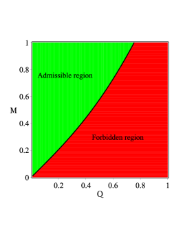
(a) $\beta=0.1$ and $\omega=-0.5$

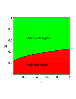
(b) $Q=0.2$ and $\omega=-0.5$

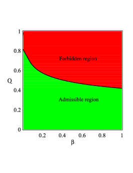
(c) $M=1$ and $\omega=-0.5$

Figure 3: The admissible parameter space for $l=1$. The black curve is the boundary for the existence of black holes in the bulk, with extremal black holes sitting on the curve.

Now, we study van der Waals phase transition by the use of definition (41). Inserting this relation into Eq. (8), one finds

$$T=\frac{1}{4\pi}\left(\frac{1}{r_{+}}-\frac{Q^{2}}{r_{+}^{3}}+\frac{3r_{+}}{l^{2}}+\frac{8\pi\beta l^{3\omega+3}}{r_{+}^{3\omega+2}}\right),$$ (48)

From Eq. (48), the equation of state $\beta(T,r_{+})$ is given by

$$\beta=\frac{Tr_{+}^{3\omega+2}}{2l^{3\omega+3}}+\frac{Q^{2}r_{+}^{3\omega-1}}{8\pi l^{3\omega+3}}-\frac{r_{+}^{3\omega+1}}{8\pi l^{3\omega+3}}-\frac{3r_{+}^{3\omega+3}}{8\pi l^{3\omega+5}},$$ (49)

where for $\omega=-1$, Eq. (49) reduces to

$$\beta=\frac{T}{2r_{+}}+\frac{Q^{2}}{8\pi r_{+}^{4}}-\frac{1}{8\pi r_{+}^{2}}-\frac{3}{8\pi l^{2}},$$ (50)

Substituting Eq. (41) in Eq. (4) and differentiating with respect to $\beta$, one can obtain conjugate quantity of $\beta$ as

$$\chi=\frac{\partial M}{\partial\beta}=\frac{4\pi l^{3\omega+3}}{3|\omega|r_{+}^{3\omega}}.$$ (51)

According to dimensional analysis, it is worth mentioning that we can match $\beta$ and $\chi$ to ad hoc pressure ($[\beta]=[length]^{-2}$) and volume ($[\chi]=[length]^{3}$), respectively. Equation (49) can be rewritten in terms of $\chi$ as

$$\beta=\frac{\mathcal{B}^{3\omega-1}\chi^{\frac{1-3\omega}{3\omega}}\left(Q^{2}l^{2}+4\pi Tl^{2}\mathcal{B}^{3}\chi^{-\frac{1}{\omega}}-\mathcal{B}^{2}l^{2}\chi^{-\frac{2}{3\omega}}-3\mathcal{B}^{4}\chi^{-\frac{4}{3\omega}}\right)}{8\pi l^{3\omega+5}},$$ (52)

where $\mathcal{B}=\left(\frac{4\pi l^{3\omega+3}}{3|\omega|}\right)^{\frac{1}{3\omega}}$. The behavior $\beta$ and $T$ as a function of $\chi$ is depicted in Fig. 4 which shows that the type of phase transition is van der Waals like. Taking a look at Figs. 4a and 4b, one can find that for $\omega<-\frac{2}{3}$, the van der Waals like phase transition occurs for $T<T_{c}$ and $\beta<\beta_{c}$, whereas for $\omega>-\frac{2}{3}$, such a behavior is possible for $T>T_{c}$ and $\beta>\beta_{c}$ (see Figs. 4c and 4d).

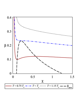
(a) $Q=0.1$ and $\omega=-0.8$

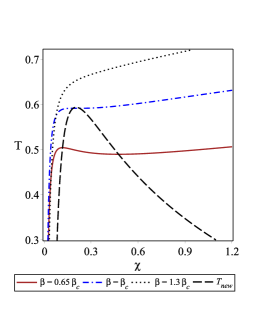
(b) $Q=0.1$ and $\omega=-0.8$

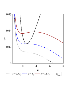
(c) $Q=0.2$ and $\omega=-0.5$

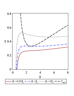
(d) $Q=0.2$ and $\omega=-0.5$

Figure 4: van der Waals like phase diagrams for $l=1$. Left panels: $\beta$ (continuous, dash-dotted and dotted line) for different temperatures and $\beta_{new}$ (dashed line) versus $\chi$. Right panels: $T$ (continuous, dash-dotted and dotted line) for different $\beta$ and $T_{new}$ (dashed line) versus $\chi$.

As we see from Figs. 4a and 4c, some parts of the isotherms corresponds to a negative $\beta$ which are not physically acceptable. It should be noted that this also occurs in the usual van der Waals fluid where the pressure can become negative for certain values of $T$. This oscillating part of the isotherm indicates instability region ($\frac{\partial\beta}{\partial\chi}>0$). Indeed, to observe an acceptable behavior, $\beta$ should be a decreasing function of $\chi$. In any place that such a principle is violated, the BH is unstable and may undergo a phase transition in that region. In order to see whether $\beta$ is a decreasing/increasing function of its conjugate quantity, we calculate its first order derivation with respect to $\chi$

$$\frac{d\beta}{d\chi}=\frac{l^{2}\left(Q^{2}\mathcal{B}^{3\omega-2}(3\omega-1)\chi^{\frac{2-3\omega}{3\omega}}+4\pi T\mathcal{B}^{3\omega+1}(3\omega+2)\chi^{-\frac{3\omega+1}{3\omega}}-(3\omega+1)\mathcal{B}^{3\omega}\chi^{-1}\right)-9\mathcal{B}^{3\omega+2}(\omega+1)\chi^{-\frac{3\omega+2}{3\omega}}}{8\pi l^{3\omega+5}},$$ (53)

If this expression is negative, the BH admits the mentioned principle and that region is physically accessible, while positivity of this expression means that a phase transition takes place in that region. It is worthwhile to mention that places where the signature of $\frac{d\beta}{d\chi}$ changes are where $\beta$ has an extremum. To express such a possibility, we have plotted diagrams in Fig. 5.

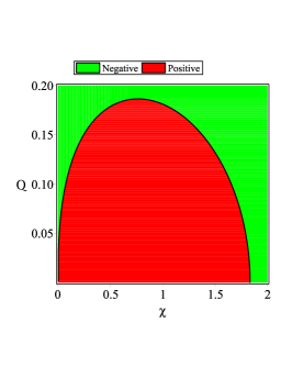
(a) $T=0.2$ and $\omega=-0.8$

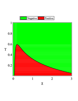
(b) $Q=0.1$ and $\omega=-0.8$

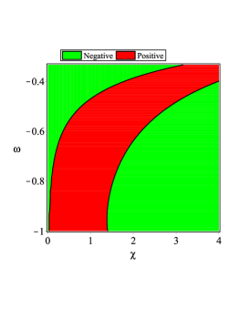
(c) $T=0.2$ and $Q=0.1$

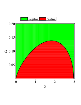
(d) $T=0.2$ and $\omega=-0.5$

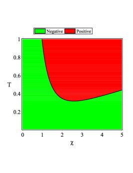
(e) $Q=0.2$ and $\omega=-0.5$

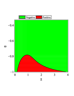
(f) $T=0.2$ and $Q=0.2$

Figure 5: Variation of the $(\frac{d\beta}{d\chi})$ as a function of different parameters for $l=1$.

To get more information about the phase transition, we investigate $G-T$ diagram. The Gibbs free energy in the canonical ensemble can be calculated as

$$G=\frac{3Q^{2}}{4r_{+}}+\frac{r_{+}}{4}-\frac{r_{+}^{3}}{4l^{2}}-\frac{2\pi\beta(3\omega+2)l^{3+3\omega}}{3\omega r_{+}^{3\omega}},$$ (54)

where $r_{+}$ is related to $\chi$ which is a function of $T$ and $\beta$ through Eq. (52). The phase transitions of a system can be categorized by their orders which are characterized by the discontinuity in n^th derivatives of the Gibbs free energy. For example, in a first-order phase transition, $G$ is a continuous function but its first derivative (the entropy or volume) changes abruptly whereas in the second-order one, both $G$ and its first derivative are continuous and the heat capacity (the second derivative of $G$) is a discontinuous function. Formation of the swallow-tail shape in $G-T$ diagram (continuous line of Figs. 6a and 6c) represents a first-order phase transition in the system. The phase transition point is located at the cross point in the $G-T$ diagram, where small BH (SBH) and large BH (LBH) exist simultaneously (see Figs. 6a and 6c). Right panels of Fig. 6 display the coexistence line of small/large BH phase transition. The critical point is located at the end of the coexistence line which is indicated in Figs. 6b and 6d. The first-order phase transition occurs when the black hole crosses the coexistence line. Taking a look at Fig. 6a, we see that for $\omega<-\frac{2}{3}$, the first-order phase transition occurs for $\beta<\beta_{c}$, whereas for $\omega>-\frac{2}{3}$, such a phase transition is possible for $\beta>\beta_{c}$ (see Fig. 6c).

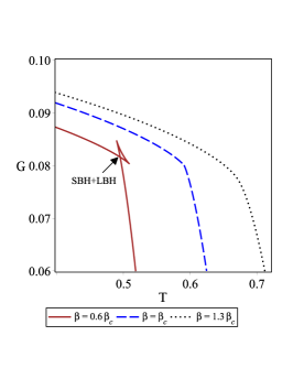
(a) $Q=0.1$ and $\omega=-0.8$

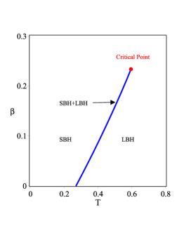
(b) $Q=0.1$ and $\omega=-0.8$

(c) $Q=0.2$ and $\omega=-0.5$

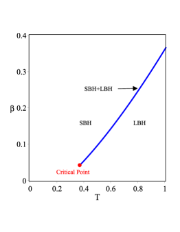
(d) $Q=0.2$ and $\omega=-0.5$

Figure 6: Left panels: the Gibbs free energy diagram $G-T$. Right panels: Coexistence curve of small-large BH phase transition in the $\beta-T$ plane.

To calculate critical values, we use the properties of inflection point which leads to

$$\chi_{c} = \mathcal{B}^{3\omega}\left(\frac{\sqrt{2l}}{6}\sqrt{\frac{l(1+3\omega)+\sqrt{108Q^{2}(1+\omega)(1-3\omega)+l^{2}(1+3\omega)^{2}}}{(1+\omega)}}\right)^{-3\omega},$$

$$T_{c} = \frac{\mathcal{B}^{2}l^{2}(3\omega+1)\chi^{\frac{1}{3\omega}}-Q^{2}l^{2}(3\omega-1)\chi^{\frac{1}{\omega}}+9\mathcal{B}^{4}(\omega+1)\chi^{-\frac{1}{3\omega}}}{4\pi(3\omega+2)\mathcal{B}^{3}l^{2}},$$

$$\beta_{c} = \frac{\mathcal{B}^{3\omega-1}\chi^{\frac{1-3\omega}{3\omega}}\left(3Q^{2}l^{2}-\mathcal{B}^{2}l^{2}\chi^{-\frac{2}{3\omega}}+3\mathcal{B}^{4}\chi^{-\frac{4}{3\omega}}\right)}{8\pi l^{3\omega+5}}.$$ (55)

To inspect the effects of electric charge and state parameter on the critical values, we have depicted Fig 7d. As we see, from Fig. 7da, for $\omega<-\frac{2}{3}$, both $T_{c}$ and $\beta_{c}$ are decreasing functions of $Q$ and vice versa (see Fig. 7dc). Regarding the effect of $\omega$ on these quantities, for $\omega<-\frac{2}{3}$, increasing the state parameter from $-1$ to $-\frac{2}{3}$ makes the increasing of $T_{c}$ and $\beta_{c}$ (see Fig. 7db), whereas for $\omega>-\frac{2}{3}$, increasing this parameter leads to the decreasing both quantities $T_{c}$ and $\beta_{c}$ (see Fig. 7dd).

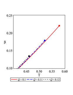
(a) $\omega=-0.8$

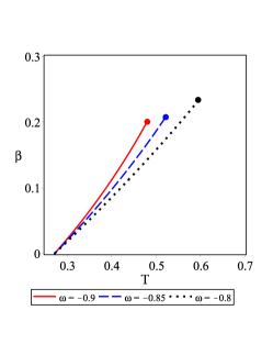
(b) $Q=0.1$

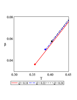
(c) $\omega=-0.5$

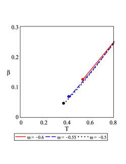
(d) $Q=0.2$

Figure 7: $\beta-T$ diagram for $l=1$, different values of electric charge (left panels) and different values of state parameter $\omega$ (right panels). Small circles in the endpoint of each line represent the critical points

.

To calculate new relation for the parameter $\beta$, we obtain the heat capacity as

$$C_{Q}=T\left(\frac{\partial S}{\partial T}\right)_{Q,\beta} = \frac{2\pi\mathcal{B}^{2}\chi^{-\frac{2}{3\omega}}\left(3\mathcal{B}^{4}\chi^{-\frac{4}{3\omega}}+\mathcal{B}^{2}l^{2}\chi^{-\frac{2}{3\omega}}-Q^{2}l^{2}+8\pi\beta\mathcal{B}^{1-3\omega}l^{3\omega+5}\chi^{\frac{3\omega-1}{3\omega}}\right)}{3\mathcal{B}^{4}\chi^{-\frac{4}{3\omega}}-\mathcal{B}^{2}l^{2}\chi^{-\frac{2}{3\omega}}+3Q^{2}l^{2}-8\pi\beta(3\omega+2)\mathcal{B}^{1-3\omega}l^{3\omega+5}\chi^{\frac{3\omega-1}{3\omega}}}.$$ (56)

Solving the denominator of the heat capacity with respect to $\beta$, a new relation is determined as follows

$$\beta_{new}=\frac{\mathcal{B}^{3\omega-1}\chi_{e}^{\frac{1-3\omega}{3\omega}}\left(3Q^{2}l^{2}-\mathcal{B}^{2}l^{2}\chi_{e}^{-\frac{2}{3\omega}}+3\mathcal{B}^{4}\chi_{e}^{-\frac{4}{3\omega}}\right)}{8\pi l^{3\omega+5}},$$ (57)

where $\chi_{e}$ indicates $\chi$ related to the extremum. The resultant curve is displayed in Fig. 4 by the dashed lines. From Fig. 4a, we see that for $\omega<-\frac{2}{3}$, the function $\beta_{new}$ has a maximum point which coincides to $\beta_{c}$, while vice versa happens for $\omega>-\frac{2}{3}$ (see Fig. 4c). Inserting Eq. (57) into the relation of temperature Eq. (48), one finds a new relation for the temperature which is independent of $\beta$

$$T_{new}=\frac{\mathcal{B}^{2}l^{2}(3\omega+1)\chi_{e}^{\frac{1}{3\omega}}-Q^{2}l^{2}(3\omega-1)\chi_{e}^{\frac{1}{\omega}}+9\mathcal{B}^{4}(\omega+1)\chi_{e}^{-\frac{1}{3\omega}}}{4\pi(3\omega+2)\mathcal{B}^{3}l^{2}},$$ (58)

the existence of extremum in the obtained relation is representing the critical temperature (see dashed lines in Figs. 4b and 4d). By deriving the new parameter $\beta$ or temperature with respect to $\chi$, one can obtain $\chi_{e}$ as

$$\frac{\partial P_{new}}{\partial\chi}=0~{}~{}~{}\Longrightarrow~{}~{}~{}\chi_{e}=\mathcal{B}^{3\omega}\left(\frac{\sqrt{2l}}{6}\sqrt{\frac{l(1+3\omega)+\sqrt{108Q^{2}(1+\omega)(1-3\omega)+l^{2}(1+3\omega)^{2}}}{(1+\omega)}}\right)^{-3\omega},$$ (59)

which is the same as $\chi_{c}$. Inserting Eq. (59) into Eqs. (58) and (57), one can find that $T_{new}$ and $\beta_{new}$ are, respectively, the same as $T_{c}$ and $\beta_{c}$ in Eq. (55).

Behavior near the critical point

Let us now compute the critical exponents for the BH system. We start with the behavior of the entropy and rewrite it in terms of $T$ and $\chi$ as

$$S(T,\chi)=\pi\mathcal{B}^{2}\chi^{-\frac{2}{3\omega}},$$ (60)

which is independent of temperature. So, we find that

$$C_{\chi}=T\frac{\partial S}{\partial T}\bigg{|}_{\chi}=0,$$ (61)

and hence $\alpha=0$.

Expanding the the equation of state around the critical point

$$\varphi=\frac{\chi}{\chi_{c}}-1,~{}~{}~{}t=\frac{T}{T_{c}}-1.$$ (62)

and defining $\varrho=\frac{\beta}{\beta_{c}}$, Eq. (52) is rewritten as

$$\varrho=\mathcal{B}_{1}+B_{1}t+\mathcal{B}_{2}\varphi t+\mathcal{B}_{3}\varphi+\mathcal{B}_{4}\varphi^{2}+\mathcal{B}_{5}\varphi^{3}+O(t\varphi^{2},\varphi^{4}),$$ (63)

where

$$\mathcal{B}_{2} = -\frac{1}{3\omega}B_{1}(2+3\omega),$$

$$\mathcal{B}_{3} = -\frac{1}{3\omega}\left(3\mathcal{B}_{1}\omega+2B_{1}-B_{2}+B_{3}+3B_{4}\right),$$

$$\mathcal{B}_{4} = \frac{1}{18\omega^{2}}\left(9\omega(2B_{1}-B_{2}+B_{3}+3B_{4})+3B_{1}+8B_{4}+\mathcal{B}_{1}+18\mathcal{B}_{1}\omega^{2}\right),$$

$$\mathcal{B}_{5} = -\frac{1}{162\omega^{3}}\left(99\omega^{2}(2B_{1}-B_{2}+B_{3}+3B_{4})+18\omega(\mathcal{B}_{1}+3B_{1}+8B_{4})+8B_{1}-B_{2}+B_{3}+27B_{4}+162\mathcal{B}_{1}\omega^{3}\right),$$ (64)

which is the same as Eq. (32), and the only difference between these two equations is $B_{i}$ coefficients given by

$$\mathcal{B}_{1} = B_{1}+B_{2}+B_{3}+B_{4},~{}~{}~{}B_{1}=\frac{T_{c}\mathcal{B}^{3\omega+2}\chi_{c}^{-\frac{3\omega+2}{3\omega}}}{2\beta_{c}l^{3\omega+3}},~{}~{}~{}B_{2}=\frac{Q^{2}\mathcal{B}^{3\omega-1}\chi_{c}^{\frac{1-3\omega}{3\omega}}}{8\pi\beta_{c}l^{3\omega+3}},$$

$$B_{3} = -\frac{\mathcal{B}^{3\omega+1}\chi_{c}^{-\frac{1+3\omega}{3\omega}}}{8\pi\beta_{c}l^{3\omega+3}},~{}~{}~{}B_{4}=-\frac{3\mathcal{B}^{3\omega+3}\chi_{c}^{-\frac{1+\omega}{\omega}}}{8\pi\beta_{c}l^{3\omega+5}}.$$ (65)

Our numerical analysis showed that the coefficients $\mathcal{B}_{3}$ and $\mathcal{B}_{4}$ are very small and can be considered zero as in the previous case. The obtained critical coefficients $\lambda$, $\gamma$ and $\delta$ are the same as those presented in the previous subsection and we do not write them here to avoid repetition. So the obtained critical exponents in this approach coincide with those obtained for van der Waals fluid, similar to the previous case.

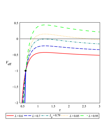
Figure 8: Effective potential $V_{eff}$ as a function of $r$ for $E=l=1$, $M=0.5$ $,\beta=0.05$, $Q=0.1$, $\omega=-0.8$ and various $L$. The blue solid line is related to the place of the horizon where $V_{eff}=-1$.

IV PHOTON SPHERE AND SHADOW

The image of a supermassive BH in the galaxy $M87$, a dark part which is surrounded by a bright ring, was direct support of the Einstein’s general relativity and the existence of the BH in our universe Akiyama . The image of the BH gives us the information regarding its jets and matter accretion. The BH shadow is one of the useful tools for a better understanding of the fundamental properties of the BH and comparing alternative theories with general relativity. The gravitational field near the black hole’s event horizon is so strong that can affect light paths and causes spherical light rings. The shadow of a BH is caused by gravitational light deflection.

It is worthwhile to mention that in preliminary studies in the context of BH shadow, the BH was assumed to be eternal, i.e, the spacetime was assumed to be time independent. So, a static or stationary observer could see a time-independent shadow. But, modern observational results have shown that our universe is expanding with acceleration. This reveals the fact that shadow depends on time. Although for the BH candidates at the center of the Milky Way galaxy and at the centers of nearby galaxies the effect of the cosmological expansion is negligible, for galaxies at a larger distance the influence on the diameter of the shadow is significant Perlick . One method to explain the amazing accelerating expansion is to introduce dark energy which makes up about $70$ percent of the universe. The cosmological constant and quintessence are two well-known candidates of dark energy scenarios. Recently, the role of the cosmological constant in gravitational lensing has been the subject of focused studies Sh1 ; Sh2 ; Sh3 ; Sh4 ; Sh5 . The BH shadow arises as a result of gravitational lensing in a strong gravity regime. So, one can inspect the effect of the cosmological constant on the shadow of black holes Sh6 ; Sh7 ; Sh8 .

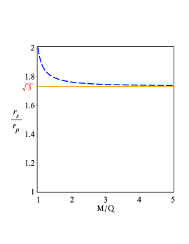
(a) RN BH

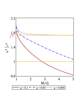
(b) RN AdS BH

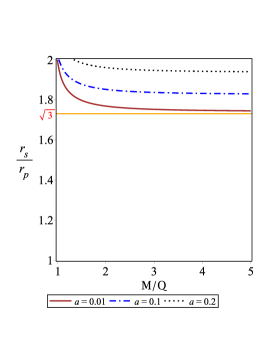
(c) RNQ BH for $\omega=-1/3$

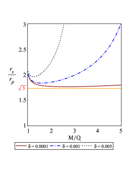
(d) RNQ BH for $\omega=-1$

Figure 9: The dependce of $\frac{r_{s}}{r_{p}}$ on the ratio $\frac{M}{Q}$. In up right panel, we consider $q=\frac{Q}{l}$. In down right panel, we set $\delta=aQ^{2}$ where $a$ is the normalization factor.

It should be noted that although the expansion of the universe was based on a positive cosmological constant, some pieces of evidence show that it can be associated with a negative cosmological constant. As we know, an interesting approach to examine the accelerated cosmic expansion and study properties of dark energy is through observational Hubble constant data which has gained significant attention in recent years Sh9 ; Sh10 ; Sh11 . The Hubble constant, $H(z)$, is measured as a function of cosmological redshift. The investigation of $H(z)$ behavior at low redshift data showed that the dark energy density has a negative minimum for certain redshift ranges which can be simply modeled through a negative cosmological constant Dutta12 . The other reason to consider a negative cosmological constant is the concept of stability of the accelerating universe. In Ref. Maedaa , authors analyzed the possibility of de Sitter expanding spacetime with a constant internal space and demonstrated that de Sitter solution would be stable just in the presence of the negative cosmological constant. The other interesting reason is through supernova data. Although there is strong observational evidence from high-redshift supernova that the expansion of the Universe is accelerating due to a positive cosmological constant, the supernova data themselves derive a negative mass density in the Universe Riess ; Perlmutter . Several galaxy cluster observations appear to have inferred the presence of a negative mass in cluster environments. It was shown that a negative mass density can be equivalent to a negative cosmological constant Farnes . In fact, the introduction of negative masses can lead to an AdS space. This would correspond to one of the most researched areas of string theory, the AdS/CFT correspondence.

Now, we would like to investigate how BH parameters affect the shadow radius of the corresponding black hole. To do so, we employ the Hamilton-Jacobi method for a photon in the BH spacetime. The Hamilton-Jacobi equation is expressed as Carter ; Decanini

$$\frac{\partial S}{\partial\sigma}+H=0,$$ (66)

where $S$ and $\sigma$ are the Jacobi action and affine parameter along the geodesics, respectively. The Hamiltonian of the photon moving in the static spherically symmetric spacetime is

$$H=\frac{1}{2}g^{\mu\nu}\frac{\partial S}{\partial x^{\mu}}\frac{\partial S}{\partial x^{\nu}}=0.$$ (67)

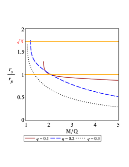
(a) $\sigma=0.001$ and $\omega=-1/3$

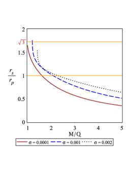
(b) $q=0.2$ and $\omega=-1/3$

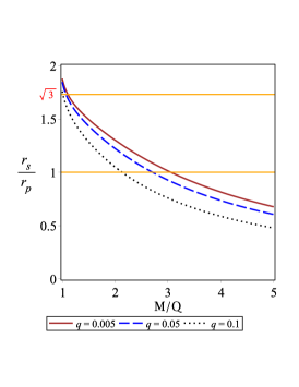
(c) $\sigma=0.001$ and $\omega=-1$

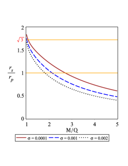
(d) $q=0.1$ and $\omega=-1$

Figure 10: The dependce of $\frac{r_{s}}{r_{p}}$ on the ratio $\frac{M}{Q}$. We have set $q=\frac{Q}{l}$ and $\sigma=\beta Q^{2}$.

Due to the spherically symmetric property of the black hole, one can consider a photon motion on the equatorial plane with $\theta=\frac{\pi}{2}$. So, Eq. (67) reduces to

$$\frac{1}{2}\left[-\frac{1}{f(r)}\left(\frac{\partial H}{\partial\dot{t}}\right)^{2}+f(r)\left(\frac{\partial H}{\partial\dot{r}}\right)^{2}+\frac{1}{r^{2}}\left(\frac{\partial H}{\partial\dot{\phi}}\right)^{2}\right]=0.$$ (68)

Regarding the fact that the Hamiltonian does not depend explicitly on the coordinates $t$ and $\phi$, one can define

$$\frac{\partial H}{\partial\dot{t}}=-E~{}~{}~{}~{}and~{}~{}~{}~{}\frac{\partial H}{\partial\dot{\phi}}=L,$$ (69)

where constants $E$ and $L$ are, respectively, the energy and angular momentum of the photon. Using the Hamiltonian formalism, the equations of motion are obtained as

$$\dot{t}=\frac{dt}{d\sigma}=-\frac{1}{f(r)}\left(\frac{\partial H}{\partial\dot{t}}\right)~{}~{}~{},~{}~{}~{}\dot{r}=\frac{dr}{d\sigma}=-f(r)\left(\frac{\partial H}{\partial\dot{r}}\right)~{}~{}~{},~{}~{}~{}\dot{\phi}=\frac{d\phi}{d\sigma}=\frac{1}{r^{2}}\left(\frac{\partial H}{\partial\dot{\phi}}\right).$$ (70)

The effective potential of the photon is obtained as

$$\dot{r}^{2}+V_{eff}(r)=0~{}~{}~{}\Longrightarrow~{}~{}~{}V_{eff}(r)=f(r)\left[\frac{L^{2}}{r^{2}}-\frac{E^{2}}{f(r)}\right].$$ (71)

Figure 8 depicts the behavior of the photon’s effective potential for $E=1$ with various $L$. As we see, there exists a peak of the effective potential which increases with increasing $L$. Due to the constraint $\dot{r}^{2}\geq 0$, we expect that the effective potential satisfies $V_{eff}\leq 0$. So, an ingoing photon from infinity with the negative effective potential falls into the BH inevitably, whereas it bounces back if $V_{eff}>0$. An interesting occurrence is related to the critical angular momentum $L=L_{p}$ ($V_{max~{}eff}=0$). In this case, the ingoing photon loses both its radial velocity and acceleration at $r=r_{max}$ completely. But for the sake of its non-vanishing transverse velocity, it can circle the black hole. So, the case of $r=r_{max}$ is called the photon orbit and it is denoted as $r=r_{p}$. From what was expressed, one can find that the photon orbits are circular and unstable associated to the maximum value of the effective potential. In order to obtain such a maximum value, we use the following conditions, simultaneously

$$V_{eff}(r)\Bigg{|}_{r=r_{p}}=0,~{}~{}~{}~{}~{}\frac{\partial V_{eff}(r)}{\partial r}\Bigg{|}_{r=r_{p}}=0,~{}~{}~{}~{}~{}~{}\frac{\partial^{2}V_{eff}(r)}{\partial r^{2}}\Bigg{|}_{r=r_{p}}<0,$$ (72)

where the first two conditions, determining the critical angular momentum of the photon sphere ($L_{p}$) and the photon sphere radius ($r_{p}$), respectively, result in the following equation

$$\frac{4Q^{2}}{r_{p}^{5}}-\frac{6M}{r_{p}^{4}}+\frac{2}{r_{p}^{3}}-\frac{8\pi\beta(\omega+1)l^{3\omega+3}}{\omega r_{p}^{3\omega+4}}=0.$$ (73)

Besides, the third condition ensures that the photon orbits are unstable. The orbit equation for the photon is obtained in the following form

$$\frac{dr}{d\phi}=\frac{\dot{r}}{\dot{\phi}}=\frac{r^{2}f(r)}{L}\left(\frac{\partial H}{\partial\dot{r}}\right).$$ (74)

The turning point of the photon orbit is expressed by the following constraint

$$\frac{dr}{d\phi}\Bigg{|}_{r=R}=0.$$ (75)

Using Eqs. (68) and (75), one gets

$$\frac{dr}{d\phi}=\pm r\sqrt{f(r)\left[\frac{r^{2}f(R)}{R^{2}f(r)}-1\right]}.$$ (76)

Considering a light ray sending from a static observer placed at $r_{0}$ and transmitting into the past with an angle $\Theta$ with respect to the radial direction, one can write M.Zhang ; Belhaj

$$\cot\Theta=\frac{\sqrt{g_{rr}}}{g_{\phi\phi}}\frac{dr}{d\phi}\Bigg{|}_{r=r_{0}}.$$ (77)

Hence, the shadow radius of the BH can be obtained as

$$r_{s}=r_{0}\sin\Theta=R\sqrt{\frac{f(r_{0})}{f(R)}}\Bigg{|}_{R=r_{p}},$$ (78)

where $r_{0}$ is the position of the observer.

Table 2: The event horizon, photon sphere radius and shadow radius for the variation of the total mass, the electric charge, the state parameter and the parameter $\beta$ for $l=1$.

$M$	$0.2$	$0.25$	$0.3$	$0.35$
$r_{e}(Q=0.1$, $\beta=0.01$ and $\omega=-0.8$)	$0.24$	$0.32$	$0.39$	$0.46$
$r_{p}(Q=0.1$, $\beta=0.01$ and $\omega=-0.8$)	$0.39$	$0.55$	$0.7$	$0.85$
$r_{s}(Q=0.1$, $\beta=0.01$ and $\omega=-0.8$)	$0.56$	$0.68$	$0.75$	$0.8$
$Q$	$0.01$	$0.05$	$0.1$	$0.15$
$r_{e}(\beta=0.01$, $M=0.3$ and $\omega=-0.8$)	$0.42$	$0.41$	$0.399$	$0.37$
$r_{p}(\beta=0.01$, $M=0.3$ and $\omega=-0.8$)	$0.730$	$0.721$	$0.708$	$0.671$
$r_{s}(\beta=0.01$, $M=0.3$ and $\omega=-0.8$)	$0.762$	$0.761$	$0.754$	$0.743$
$\beta$	$0.01$	$0.02$	$0.04$	$0.06$
$r_{e}(Q=0.1$, $M=0.3$ and $\omega=-0.8$)	$0.398$	$0.392$	$0.37$	$0.36$
$r_{p}(Q=0.1$, $M=0.3$ and $\omega=-0.8$)	$0.70$	$0.69$	$0.67$	$0.65$
$r_{s}(Q=0.1$, $M=0.3$ and $\omega=-0.8$)	$0.75$	$0.72$	$0.68$	$0.64$
$\omega$	$-1$	$-0.9$	$-0.8$	$-0.7$
$r_{e}(Q=0.1$, $M=0.3$ and $\beta=0.01$)	$0.403$	$0.402$	$0.399$	$0.395$
$r_{p}(Q=0.1$, $M=0.3$ and $\beta=0.01$)	$0.722$	$0.716$	$0.708$	$0.696$
$r_{s}(Q=0.1$, $M=0.3$ and $\beta=0.01$)	$0.764$	$0.760$	$0.754$	$0.747$

Since Eqs. (73) and (78) are complicated to solve analytically, we employ numerical methods to obtain the radius of the photon sphere and shadow. In this regard, several values of the event horizon ($r_{e}$), photon sphere radius ($r_{p}$) and shadow radius ($r_{s}$) are presented in Table 2. We find that for intermediate values of the total mass, the photon sphere radius would be larger than the shadow radii which is physically not acceptable. To have a physical behavior, we consider the small mass for our investigation. We note that the size of shadow shrinks with increasing the electric charge and parameter $\beta$. Regarding the effect of state parameter, we find that increasing this parameter from $-1$ to $-2/3$ results in a decrease of the photon sphere and shadow radius.

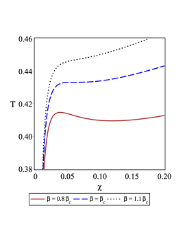
(a)

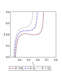
(b)

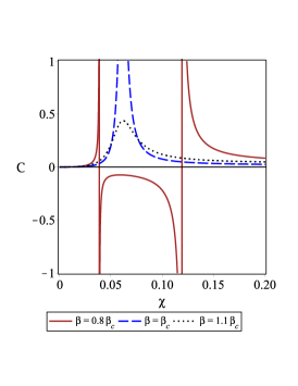
(c)

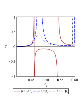
(d)

Figure 11: Hawking temperature with respect to $\chi$ (up-left panel) and $r_{s}$ (up-right panel); The heat capacity versus $\chi$ (down-left panel) and $r_{s}$ (down-right panel) for $l=1$, $Q=0.1$, $\omega=-1$ and various $\beta$.

As it was already mentioned, no acceptable optical behavior is observed for large values of total mass. This shows that a restriction between the total mass and electric charge should be imposed to observe an acceptable physical result. To have a better understanding of this issue, we examine the ratio of shadow radius and photon sphere ($\frac{r_{s}}{r_{p}}$) for two limited states, $\omega=-\frac{1}{3}$ and $\omega=-1$. For more precise study, we first inspect this ratio for three BH solutions as the Reissner-Nordström (RN) BH, RN - AdS BH and RN BH in the presence of quintessence. The qualitative behavior of the ratio $\frac{r_{s}}{r_{p}}$ with respect to $\frac{M}{Q}$ is displayed in Fig. 9. From this figure, one can find that the proposed inequality relationship ($\frac{r_{s}}{r_{p}}\geq\sqrt{3}$) in Ref. HDLyu is satisfied for charged BH (see Fig. 9a) and charged one in the quintessence (see Figs. 9c and 9d), whereas for RN - AdS BH, as we see from Fig. 9b, this ratio is fulfill just for very small values of $q=\frac{Q}{l}$ (for small electric charge or large AdS radius). Figure 9 also shows that the ratio $\frac{r_{s}}{r_{p}}$ monotonically decreases as the ratio $\frac{M}{Q}$ increases. This means that the increase of difference between the values of total mass and electric charge will make the ratio $\frac{r_{s}}{r_{p}}$ decrease. Only for RN black hole in the presence of quintessence with $\omega=-1$, the ratio $\frac{r_{s}}{r_{p}}$ increases by increasing the ratio $\frac{M}{Q}$, however for very small values of $\delta=aQ^{2}$ (for small electric charge and normalization factor), the ratio $\frac{r_{s}}{r_{p}}$ is a decreasing function of $\frac{M}{Q}$.

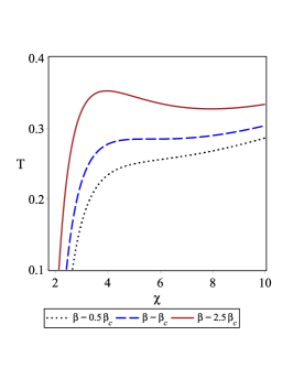
(a)

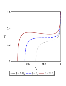
(b)

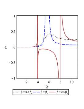
(c)

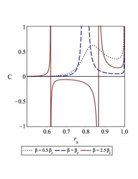
(d)

Figure 12: Hawking temperature with respect to $\chi$ (up-left panel) and $r_{s}$ (up-right panel); The heat capacity versus $\chi$ (down-left panel) and $r_{s}$ (down-right panel) for $l=1$, $Q=0.2$, $\omega=-1/3$ and various $\beta$.

Now, we would like to investigate qualitative behavior of the ratio $\frac{r_{s}}{r_{p}}$ for our solution. From Eq. (73), the radius of photon sphere can be obtained as

$$r_{p} = \frac{3M+\sqrt{9M^{2}+8Q^{2}-64\pi\beta Q^{2}l^{2}}}{2(8\pi\beta l^{2}+1)}~{}~{}~{}~{}\omega=-\frac{1}{3},$$ (79)

$$r_{p} = \frac{3}{2}M+\frac{1}{2}\sqrt{9M^{2}-8Q^{2}}~{}~{}~{}~{}~{}~{}~{}~{}~{}~{}~{}~{}~{}~{}~{}~{}~{}~{}\omega=-1.$$ (80)

Inserting $r_{p}$ into Eq. (78), one can obtain the radius of shadow. The ratio $\frac{r_{s}}{r_{p}}$ with respect to $\frac{M}{Q}$ is depicted in Fig. 10. Taking a look at this figure, one can find that the inequality relationship $\frac{r_{s}}{r_{p}}\geq\sqrt{3}$ is not fulfill for RN-AdS BH in the presence of quintessence. Moreover for large $\frac{M}{Q}$, the radius of the photon sphere would be larger than the shadow radii which is not physically acceptable.

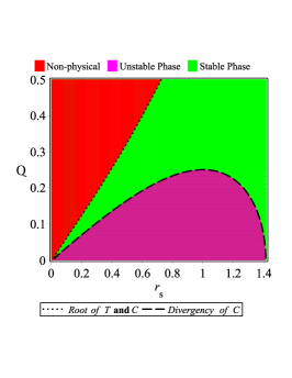
(a) $Q=0.2$ and $\omega=-1/3$

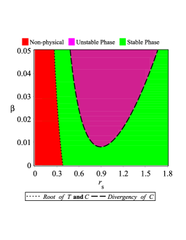
(b) $Q=0.2$ and $\omega=-1/3$

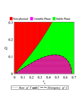
(c) $Q=0.1$ and $\omega=-1$

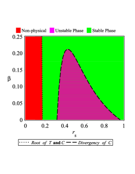
(d) $Q=0.1$ and $\omega=-1$

Figure 13: Thermally stable and/or unstable regions of the black holes for $l=1$.

IV.1 Relations between shadow radius and phase transitions

Now, we are interested in examining the relations between the shadow radius and phase transitions. According to M.Zhang ; Belhaj ; Wei2 ; Li2 , there is a close connection between BH shadows and the BH thermodynamics. The heat capacity is one of the interesting thermodynamic quantities which provides the information related to the thermal stability and phase transition of a thermodynamic system. The sign of heat capacity determines thermal stability/instability of black holes. The positivity (negativity) of this quantity indicates a BH is thermally stable (unstable). Besides, the discontinuities in heat capacity could be interpreted as the possible phase transition points. Indeed, the phase transition points are where heat capacity diverges. According to Eq. (56), heat capacity can be written as

$$C=T\left(\frac{\partial S}{\partial r_{+}}\frac{\partial r_{+}}{\partial T}\right).$$

By using the fact that $\frac{\partial S}{\partial r_{+}}>0$, the sign of $C$ is directly inducted from $\frac{\partial T}{\partial r_{+}}$ which can be rewritten as

$$\frac{\partial T}{\partial r_{+}}=\frac{\partial T}{\partial r_{s}}\frac{\partial r_{s}}{\partial r_{+}}.$$

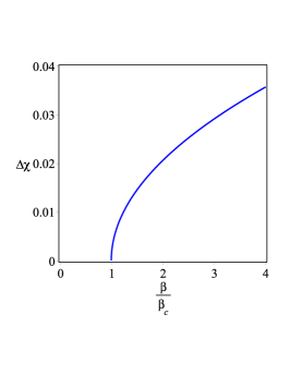
(a) $Q=0.2$ and $\omega=-1/3$

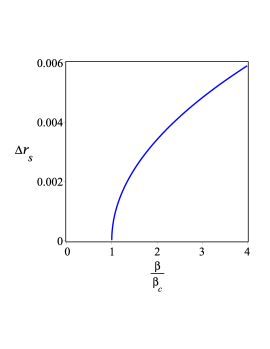
(b) $Q=0.2$ and $\omega=-1/3$

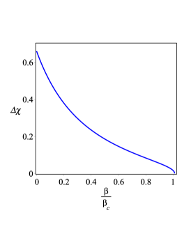
(c) $Q=0.1$ and $\omega=-1$

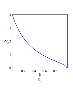
(d) $Q=0.1$ and $\omega=-1$

Figure 14: Behavior of $\Delta\chi$ and $\Delta r_{s}$ as a function of the $\frac{\beta}{\beta_{{}_{c}}}$ for $l=1$.

By satisfying the constraint $\frac{\partial r_{s}}{\partial r_{+}}>0$ M.Zhang ; Belhaj , one can draw a conclusion that the sign of $C$ is controlled by $\frac{\partial T}{\partial r_{s}}$. To investigate the link between phase transition and shadow of the black hole, we consider the temperature expression Eq. (48) and the heat capacity Eq. (56), and examine the behavior of temperature and heat capacity with respect to $r_{s}$. Since the thermodynamic behavior of the system is different for $\omega>-\frac{2}{3}$ and $\omega<-\frac{2}{3}$, we consider $\omega$ toward $-1$ and $-\frac{1}{3}$ as two limited states and solve the problem analytically. The isobar curves on the $T-r_{s}$ and $C-r_{s}$ are displayed in Figs. 11b and 11d for $\omega=-1$. As we see, these curves exhibit similar behaviors as $T-\chi$ and $C-\chi$ curves in Figs. 11a and 11c. For $\beta>\beta_{c}$, the temperature is only a monotone increasing function of $r_{s}$ without any extremum (see dotted line in Fig. 11b). The heat capacity is also a continuous function for variable $r_{s}$ (see dotted line in Fig. 11d). For the case $\beta<\beta_{c}$, a non-monotonic behavior appears for temperature with one local maximum and one minimum which corresponds to the first-order phase transition. According to the definition of heat capacity, these extrema coincide with divergence points of $C$. Evidently, a change of signature occurs at these points. In other words, it changes from positive to negative at the first divergency and then it becomes positive again at the second one. For $\omega=-1/3$, $T-r_{s}$ and $C-r_{s}$ diagrams are plotted in Fig. 12. Evidently, its behavior is opposite to $\omega=-1$ case, meaning that divergency is appeared for $\beta>\beta_{c}$, whereas a monotonic behavior is observed for $\beta<\beta_{c}$. So, three black holes are thermodynamically competing. Small black holes which are located between root and smaller divergency of the heat capacity are in a stable phase. For an intermediate range of the shadow radius, the black holes are thermodynamically unstable. The region after larger divergency is related to large black holes which are thermally stable. Figure 13 displays these three phases and the effect of BH parameters on these regions. As we see, the parameter $\beta$ (normalization factor) and state parameter have significant effects on the stability/instability of the black hole. In other words, a stable BH may exit in its stable state when it is surrounded by quintessence. This reveals the fact that it is logical to consider the normalization factor as a variable quantity.

For $\beta=\beta_{c}$, the small BH and the large one merge into one squeezing out the unstable black hole. This can be found as a deflection point in the $T-r_{s}$ plot which forms critical point of the second-order phase transition. Such behavior of temperature is very similar to van der Waals liquid-gas system which goes under a second-order phase transition at $T=T_{c}$. One can analyze the behavior of the shadow radius before and after the second-order small-large BH phase transition. To do so, we have depicted the changes of the shadow radius ($\Delta r_{s}=r_{s}^{L}-r_{s}^{S}$) as a function of the reduced $\beta$ ($\beta/\beta_{c}$) in left panels of Fig. 14. We see that $\Delta r_{s}$ and $\Delta\chi$ have similar behaviors and they are monotonically decreasing functions of the reduced parameter $\beta$. They approach to zero at $\beta=\beta_{c}$, where the first-order phase transition becomes a second-order one.

V conclusion

In this paper, we have studied the analogy of charged AdS black holes surrounded by quintessence with van der Waals fluid system with a new viewpoint, in which we kept the cosmological constant as a constant parameter and instead allow the normalization factor to vary as a thermodynamic quantity. The obtained results showed that for $\omega<-2/3$, the system has similar thermodynamic behavior as the van der Waals fluid system such that it goes under a first order phase transition for $T<T_{c}$ and $\beta<\beta_{c}$, and undergoes a second-order phase transition at $T=T_{c}$ and $\beta=\beta_{c}$. For $\omega>-2/3$, an opposite behavior was observed, meaning that a first order phase transition takes place for $T>T_{c}$ and $\beta>\beta_{c}$. We also derived all the critical exponents of the system and found that they are exactly coincident with the van der Waals fluid system.

It is worthwhile to mention that although one can investigate phase transition of a BH with help of $P-V$ and $Q^{2}-\Psi$ planes, it is more logical to take the normalization factor, which indicates the intensity of the quintessence field as a variable quantity. As we know, the cosmological constant does not change and basically has a constant value. In contrast, the quintessence field is a dynamic parameter that changes over time. Regarding the consideration the square of the electric charge as a thermodynamic quantity, although one can employ this method to explore phase transition, it should be noted that according to Dehyadegari ; Yazdikarimi a first-order phase transition takes place for temperatures above its critical values which is a little different from the behavior of van der Waals fluid and other ordinary phase transitions in everyday systems. In addition, since the electromagnetic repulsion in compressing an electrically charged mass is dramatically greater than the gravitational attraction, it is not expected that black holes with a significant electric charge will be formed in nature. So, the electric charge of a BH cannot change over the time so much.

Finally, we investigated the photon sphere and the shadow observed by a distant observer. We found that the shadow size shrinks with increasing the electric charge, state parameter $\omega$ and parameter $\beta$ (normalization factor). We also explored the connection between shadow radius and phase transition and found that for $\omega>-2/3$ ($\omega<-2/3$) there exists a non-monotonic behavior of the shadow radius for $\beta>\beta_{c}$ ($\beta<\beta_{c}$) which corresponds to a first-order phase transition. We have shown such a phase transition becomes a second-order one at $\beta_{c}$. Studying thermal stability of the system in this point of view, we noticed that the normalization factor and state parameter have a significant influence on the stability/instability of the black hole. This revealed the fact that a stable BH may exit in its stable state if it is surrounded by the quintessence.

VI Acknowledgements

We would like to thank the anonymous referees for their constructive comments. SHH also thank Shiraz University Research Council.

References

- (1) LIGO scientific collaboration, Phys. Rev. Lett. 118, 221101 (2017).
- (2) J. M. Bardeen, B. Carter, S. Hawking, Commun. Math. Phys. 31, 161 (1973) .
- (3) S. Hawking, Commun. Math. Phys. 43, 199 (1975).
- (4) J. Maldacena, Adv. Theor. Math. Phys. 2, 231 (1998).
- (5) E. Witten, Adv. Theor. Math. Phys. 2, 253 (1998).
- (6) S. Hawking and D. N. Page, Commun. Math. Phys. 87, 577 (1983).
- (7) M. Cvetic and S. S. Gubser, JHEP 04, 024 (1999).
- (8) M. Cvetic and S. Gubser, JHEP 07, 010 (1999).
- (9) D. Kubiznak and R. B. Mann, JHEP 07, 033 (2012).
- (10) D. Kubiznak and R. B. Mann and M. Teo, Class. Quant. Gravit. 34, 063001 (2017).
- (11) C. V. Johnson, Class. Quant. Gravit. 31, 205002 (2014).
- (12) A. Karch and B. Robinson, JHEP 12, 073 (2015).
- (13) R. B. Mann, Springer Proc. Phys. 170, 197 (2016).
- (14) S. Gunasekaran, R. B. Mann and D. Kubiznak, JHEP 11, 110 (2012).
- (15) N. Altamirano, D. Kubiznak, R. B. Mann and Z. Sherkatghanad, Class. Quant. Gravit. 31, 042001 (2014).
- (16) S. W. Wei and Y. X. Liu, Phys. Rev. D 90, 044057 (2014).
- (17) N. Altamirano, D. Kubiznak and R. B. Mann, Phys. Rev. D 88, 101502 (2013).
- (18) B. P. Dolan, Phys. Rev. D 84, 127503 (2011).
- (19) B. P. Dolan, A. Kostouki, D. Kubiznak and R. B. Mann, Class. Quant. Gravit. 31, 242001 (2014).
- (20) S. H. Hendi and M. H. Vahidinia, Phys. Rev. D 88 084045 (2013).
- (21) M. Zhang, Z. Y. Yang, D. C. Zou, W. Xu and R. H. Yue, Gen. Relat. Gravit. 47, 14 (2015).
- (22) K. Hristov, C. Toldo and S. Vandoren, Phys. Rev. D 88 026019 (2013).
- (23) S. Dutta, A. Jain and R. Soni, JHEP 12, 060 (2013).
- (24) S. Chen, X. Liu, C. Liu and J. Jing, Chin. Phys. Lett. 30, 060401 (2013).
- (25) E. Caceres, P. H. Nguyen and J. F. Pedraza, JHEP 09, 184 (2015).
- (26) R. A. Hennigar, W. G. Brenna and R. B. Mann, JHEP 07, 077 (2015).
- (27) W. Xu and L. Zhao, Phys. Lett. B 736, 214 (2014).
- (28) M. S. Ma, F. Liu and R. Zhao, Class. Quant. Gravit. 31, 095001 (2014).
- (29) W. G. Brenna, R. B. Mann and M. Park, Phys. Rev. D 92, 044015 (2015).
- (30) Kh. Jafarzade and J. Sadeghi, Int. J. Mod. Phys. D 26, 1750138 (2017).
- (31) J. X. Mo, X. X. Zeng, G. Q. Li, X. Jiang and W. B. Liu, JHEP 10, 056 (2013).
- (32) H. Hendi, R. B. Mann, S. Panahiyan, and B. Eslam Panah, Phys. Rev. D 95, 021501 (2017).
- (33) A. Chamblin, R. Emparan, C. Johnson, and R. Myers, Phys. Rev. D 60, 104026 (1999).
- (34) A. Chamblin, R. Emparan, C. Johnson, and R. Myers, Phys. Rev. D 60, 064018 (1999).
- (35) A. Dehyadegari, A. Sheykhi, A. Montakhab, Phys. Lett. B 768, 02064 (2017).
- (36) H. Yazdikarimi, A. Sheykhi and Z. Dayyani, Phys. Rev. D 99, 124017 (2019).
- (37) N. Bachall, J. Ostriker, S. Perlmutter and P. Steinhardt, Science 284, 1481 (1999).
- (38) V. Sahni and A. Starobinsky, Int. J. Mod. Phys. D 9, 373 (2000).
- (39) V. Kiselev, Class. Quant. Gravit. 20, 1187 (2003).
- (40) S. G. Ghosh, Eur. Phys. J. C 76, 222 (2016).
- (41) T. Oteev, A. Abdujabbarov, Z. Stuchlik and B. Ahmedov, Astrophys. Space Sci. 361, 269 (2016).
- (42) B. Toshmatov, Z. Stuchlik, and B. Ahmedov, arXiv:1512.01498 [gr-qc].
- (43) Z. Xu and J. Wang, Phys. Rev. D 95, 064015 (2017).
- (44) B. Majeed, M. Jamil and P. Pradhan, Adv. High Energy Phys. 2015, 124910 (2015).
- (45) Z. Xu and J. Wang, Int. J. Mod. Phy A 30, 1950185 (2019).
- (46) G. Q. Li, Phys. Lett. B 735, 256 (2014).
- (47) H. Liu and X. H. Meng, Eur. Phys. J. C 77, 556 (2017).
- (48) W. Hong, B. Mu and J. Tao, Nucl. Phys. B 949, 114826 (2019).
- (49) X-Y. Guo, H-F. Li, L-C. Zhang and R. Zhao, Eur. Phys. J. C 80, 168 (2020).
- (50) M. Chabab, H. El Moumni, S. Iraoui, K. Masmar and S. Zhizeh, Int. J. Geom. Meth. Mod. Phys. 15, 1850171 (2018).
- (51) S. H. Hendi, S. Panahiyan, B. Eslam Panah and M. Jamil, Chinese Phys. C 43, 113106 (2019).
- (52) S. H. Hendi, S. Panahiyan, and B. Eslam Panah, Int. J. Mod. Phys. D 25, 1650010 (2016).
- (53) K. Akiyama et al. (Event Horizon Telescope), Astrophys. J. 875, L1 (2019).
- (54) V. Perlick, O. Y. Tsupko and G. S. Bisnovatyi-Kogan, Phys. Rev. D 97, 104062 (2018).
- (55) O. F. Piattella, Phys. Rev. D 93, 024020 (2016).
- (56) L. M. Butcher, Phys. Rev. D 94, 083011 (2016).
- (57) V. Faraoni and M. Lapierre-Leonard, Phys. Rev. D 95, 023509 (2017).
- (58) H. J. He and Z. Zhang, JCAP 1708 036 (2017).
- (59) F. Zhao and J. Tang, Phys. Rev. D 92, 083011 (2015).
- (60) S. Haroon, M. Jamil, K. Jusufi, K. Lin and R. B. Mann, Phys. Rev. D 99, 044015 (2019).
- (61) R. A. Konoplya, Phys. Lett. B 795, 1 (2019).
- (62) J. T. Firouzjaee and A. Allahyari, Eur. Phys. J. C 79, 930 (2019).
- (63) Z. Yi and T. Zhang, Mod. Phys. Lett. A 22, 41 (2007).
- (64) H. Wan, Z. Yi, T. Zhang and J. Zhou, Phys. Lett. B 651, 1368 (2007).
- (65) C. Ma, T. Zhang, Astrophys. J. 730, 74 (2011).
- (66) K. Dutta, Ruchika, A. Roy, A. A. Sen and M. M. Sheikh-Jabbari, Gen. Relat. Gravit. 52, 15 (2020).
- (67) K. I. Maeda and N. Ohta, JHEP 06, 095 (2014).
- (68) A. G. Riess et al, Astron. J. 116 (1998) 1009.
- (69) S. Perlmutter et al, Astrophys. J. 517 (1999) 565.
- (70) J. S. Farnes, Astron. Astrophys 620, A92 (2018).
- (71) B. Carter, Phys. Rev. 174, 1559 (1968).
- (72) Y. Decanini, A. Folacci and B. Raffaelli, Class. Quant. Gravit. 28, 175021 (2011).
- (73) M. Zhang and M. Guo, [arXiv:1909.07033 [gr-qc]].
- (74) A. Belhaj, L. Chakhchi, H. El Moumni, J. Khalloufi and K. Masmar, [arXiv:2005.05893 [gr-qc]].
- (75) H. Lu, H.D. Lyu, Phys. Rev. D 101, 044059 (2020).
- (76) S. W. Wei and Y. X. Liu, Phys. Rev. D 97, 104027 (2018).
- (77) H. Li, Y. Chen and S. J. Zhang, Nucl. Phys. B 954 114975. (2020)