AttentionDDI: Siamese Attention-based Deep Learning method for drug-drug interaction predictions

Abstract

Background Drug-drug interactions (DDIs) refer to processes triggered by the administration of two or more drugs leading to side effects beyond those observed when drugs are administered by themselves. Due to the massive number of possible drug pairs, it is nearly impossible to experimentally test all combinations and discover previously unobserved side effects. Therefore, machine learning based methods are being used to address this issue.

Methods We propose a Siamese self-attention multi-modal neural network for DDI prediction that integrates multiple drug similarity measures that have been derived from a comparison of drug characteristics including drug targets, pathways and gene expression profiles.

Results Our proposed DDI prediction model provides multiple advantages: 1) It is trained end-to-end, overcoming limitations of models composed of multiple separate steps, 2) it offers model explainability via an Attention mechanism for identifying salient input features and 3) it achieves similar or better prediction performance (AUPR scores ranging from $0.77$ to $0.92$) compared to state-of-the-art DDI models when tested on various benchmark datasets. Novel DDI predictions are further validated using independent data resources.

Conclusions We find that a Siamese multi-modal neural network is able to accurately predict DDIs and that an Attention mechanism, typically used in the Natural Language Processing domain, can be beneficially applied to aid in DDI model explainability.

Keywords drug-drug interactions  $\cdot$ side effects  $\cdot$ prediction  $\cdot$ deep learning  $\cdot$ attention

Introduction

Polypharmacy, the concurrent administration of multiple drugs, has been increasing among patients in recent years [1]. When administering multiple drugs, interactions might arise among them, often termed drug-drug interactions (DDI). The intended effect of a drug may therefore be altered by the action of another drug. These effects could lead to drug synergy, reduced efficacy or even to toxicity. Thus, DDI discovery is an important step towards improved patient treatment and safety.

It is almost impossible to conduct an empirical assessment of all possible drug pair combinations and test their propensity for triggering DDIs. Computational approaches have addressed this issue by enabling the testing of large number of drug pairs more efficiently. For instance, DeepDDI [2], a multilabel classification model, takes drug structure data as input along with drug names, in order to make DDI predictions in the form of human-readable sentences. Another model, GENN [3], a graph energy neural network, puts a focus on DDI types and estimates correlations between them. NDD [4] utilizes multiple drug similarity matrices, which are combined by Similarity Network Fusion (SNF) and finally fed through a feed-forward network for classification. Similarly, ISCMF [5] performs matrix factorization on the known DDIs in order to calculate latent matrices which are used for predictions. It utilizes the same SNF-fused matrix as to constrain this factorization.

The above mentioned solutions come with some drawbacks. First, there is a plethora of drug feature information available for many approved drugs, including chemical structure, side effects, targets, pathways, and more. However, current DDI prediction solutions often only take advantage of a small subset of these features, particularly drug chemical structure features, due to their broad availability. Other current model limitations include low interpretability and/or the fact that they consist of multiple separate steps (i.e., cannot be trained end-to-end). A novel solution should preferably offer a mechanism to tackle those drawbacks simultaneously.

To this end, we introduce AttentionDDI, a Siamese self-attention multi-modal neural network model for DDI prediction. Our model is inspired by and adapts ideas from Attention-based models (i.e., Transformer network) [6] that showed great success particularly in the Natural Language Processing (NLP) domain. Our model 1) is trained end-to-end, 2) offers model explainability and 3) achieves similar or better prediction performance compared to state-of-the-art DDI models when tested on various benchmark datasets.

Methods

Benchmark datasets

In order to predict interactions between drugs, we focused on specific benchmark datasets listed in Table 1. Our model, AttentionDDI, and two competitive baseline models (developed by the same group), NDD [4] and ISCMF [5], are all built to take advantage of the multi-modality contained in those datasets. Each dataset consists of one or more drug similarity matrices as described in Table 1. Those matrices are calculated based on various drug feature vectors, encoding diverse drug characteristics, including, for example, the side effects that are induced by a drug or the biological pathways a drug is targeting. All together, the drug similarity matrices are based on the following drug characteristics: chemical structure, targets, pathways, transporter, enzyme, ligand, indication, side effects, offside effects, GO terms, PPI distance, and ATC codes. The datasets have been previously used by multiple other studies [7, 8, 9, 4, 5].

Additionally to the above mentioned matrices, we calculate the Gaussian Interaction Profile (GIP) similarity matrix (according to [10]) based on the interaction labels of each dataset (Table 2). Therefore, in addition to the similarity features listed in Table 1, the GIP of each dataset label matrix is also utilized as a further similarity feature. This method works under the hypothesis that drugs with resembling existing labels (DDIs) are expected to have comparable novel interaction predictions.

Dataset	$\#$ drugs	Similarity Matrices
DS1 [7]	548	Chemical, Enzyme, Indication, Offside effects, Pathway, Side effects, Target, Transporter
DS2 [8]	707	Chemical
DS3 [9]	807	ATC, Chemical, GO, Ligand, PPI Distance, Side effects, Target

Table 1: Benchmark datasets.

We obtained the precomputed drug similarity matrices from [4]. As an example, the side effects matrix of the DS1 dataset [7] was constructed as follows: A matrix representing a list of $N$ known drugs on the $y$-axis and a list of $M$ known side effects on the $x$-axis was created. In this matrix, each row is representing a drug along with its side effects in the $N\times M$ matrix. It is filled with the value $1$ in each position where it is known that a drug may cause a specific side effect, $0$ otherwise. In this fashion, each drug is represented by a binary feature vector (size $M$). Furthermore, this binary feature matrix was transformed into a similarity matrix using all drug pairs. Given two drugs, $d_{a}$ and $d_{b}$, and their binary feature vectors ($u_{a}$ and $u_{b}$ $\in[0,1]^{M}$), their similarity was calculated according to the Jaccard score:

$$J(u_{a},u_{b})=M_{11}/(M_{01}+M_{10}+M_{11}),$$

$$0\leq J(u_{a},u_{b})\leq 1$$

where $M_{01}$ represents the count of positions ($i\in[1,\cdots,M]$) in $u_{a}$ and $u_{b}$ where $u_{ai}=0$ and $u_{bi}=1$. Similarly, $M_{10}$ represents the count of positions ($i$) in $u_{a}$ and $u_{b}$ where $u_{ai}=1$ and $u_{bi}=0$. Lastly, $M_{11}$ denotes the count of positions ($i$) in $u_{a}$ and $u_{b}$ where $u_{ai}=1$ and $u_{bi}=1$. This similarity measure is calculated for each drug pair resulting in a $N\times N$ similarity matrix.

DS2 and DS3 were generated by similar approaches. The description of the similarity matrix constructions can be found in [7] for the DS1 similarity matrices, in [8] for DS2 and in [9] for DS3.

Database DDI labels

In a supervised classification setting, labels of known drug-drug interactions are required in the form of a binary matrix with the same dimensions ($N\times N$) as the input similarity matrices (Table 2). For example, the labels in DS1 were provided by the TWOSIDES database [11].

Notably, the DS3 dataset labels are split based on whether the DDIs result from a shared CYP metabolizing enzyme (CYP) or not (NCYP). This separation was made on the grounds that CYPs are major enzymes involved in $\sim 75\%$ of the total drug metabolism. As an example, one drug would inhibit a specific CYP enzyme which also metabolizes another drug, therefore triggering a CYP-related DDI. This separation of CYP labels can affect the model training and predictability, as the positive labels are way outnumbered by the negative ones (Table 2).

The known DDIs in these label matrices have the label value $1$. Label $0$, however, does not guarantee the absence of drug interactions for the given drug pair. An interaction in this case, may not have been observed yet, or may not have been included in the specific DDI database.

Dataset	$\#$ drugs	$\#$ drug-drug pairs	$\#$ known DDIs	$\%$ known DDIs
DS1	548	149’878	48’584	$\sim$32%
DS2	707	249’571	17’206	$\sim$7%
DS3 CYP	807	325’221	5’039	$\sim$1.5%
DS3 NCYP	807	325’221	20’452	$\sim$6%

Table 2: Labels for each dataset.

Model evaluation

The model performance is evaluated based on standardized classification metrics. We included 1) AUC-ROC and 2) AUC-PR. For consistency with previous studies, denoted by AUC, AUPR from now on. These scores are composed by the definitions in Table 3.

		True Interactions
		Positive	Negative
Predicted	Positive	$TP$	$FP$	$\textbf{Precision}=TP/(TP+FP)$
Interactions	Negative	$FN$	$TN$
		$\textbf{TPR},\textbf{Recall}=$	$\textbf{FPR}=$
		$TP/(TP+FN)$	$FP/(FP+TN)$

Table 3: Confusion matrix.

AUPR is the Area Under the Precision-Recall curve and is considered the fairer measure [4] especially when class imbalance (i.e., unequal label distribution) is prevalent in the dataset. This is notably the case when the number of positive samples (labels with value $1$) and the number of negative samples ($0$s) are significantly imbalanced. Given the low proportions of positive samples (Table 2) this is the main performance measure we focus on for the model evaluation. We furthermore computed the AUC as standard classification metric. AUC is the Area Under the TPR-FPR Curve, where TPR (also Recall) is the True Positive Rate and FPR is the False Positive Rate, as defined above.

Baseline model

We compared our model to multiple baseline models found in the literature with special focus on NDD [4] that showed high performance on DDI prediction (as reported by the authors). NDD consists of three parts: 1) In a first step, the similarity matrices are filtered based on matrix entropy scores. This aims at basing the classification only on the most informative similarity matrices and therefore excluding less informative ones using handcrafted heuristics. 2) In a second step, the remaining similarity matrices are merged into one matrix through the SNF method (i.e., using similarity network fusion algorithm) [12]. 3) Finally, the fused matrix is used as input to a feed-forward classifier network which outputs binary DDI predictions.

We re-implemented (to the best of our ability) NDD using the PyTorch deep learning library [13] for the purpose of reproducing the baseline model results. However, we were not able to reproduce the model results reported in [4] especially for DS2 and DS3 datasets. Therefore, we report the performance values cited by the author in their article [4, 5].

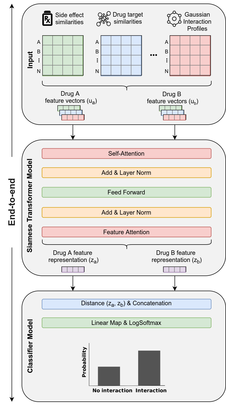
Figure 1: AttentionDDI model architecture. 1) The sets of drug pair feature vectors $(u_{a},u_{b})$ from each similarity matrix are used as model input, separately for each drug. 2) A Transformer-based Siamese encoder model generates new drug feature representation vectors for each drug. First, by applying learned weights (through Self-Attention) to the drug feature vectors. Then, by non-linearly transforming the weighted feature vectors by a feed-forward network. Finally, a Feature Attention pooling method aggregates the transformed feature vectors into a single feature vector representation for each drug ($z_{a}$ or $z_{b}$ respectively). 3) A separate classifier model concatenates the encoded feature vectors $z_{a},z_{b}$ with their distance (euclidean or cosine). Lastly, through affine mapping of the concatenated drug pair vectors followed by Softmax function, a drug-interaction probability distribution is generated for each drug pair.

AttentionDDI: Model description

We constructed a Siamese multi-head self-Attention multi-modal neural network model (Figure 1) adapting the Transformer architecture to model our DDI problem.

Siamese model

Our model is a Siamese neural network [14] designed to use the same model weights for processing in tandem two different input vectors. In our case the drug similarity features of each drug pair $(d_{a},d_{b})$ are encoded in parallel in order to learn improved latent vector representations. They are used in a later stage for computing a distance/similarity between both vectors.

Transformer architecture

Our model architecture adapts the Transformer network [6] that uses multi-head self-attention mechanism to compute new latent vector representations from the set of input vectors while being optimized during training for our DDI prediction problem. It consists of:

1. An Encoder model, which takes as input a set of drug similarity feature vectors and computes a new (unified) fixed-length feature vector representation.

2. A Classifier model, which given the new feature vector representations, generates a probability distribution for each drug pair, indicating if this drug pair is more likely to interact or not.

Input vectors

Our model is trained on each benchmark dataset (i.e., DS1, DS2 and DS3) separately. There are one or more similarity matrices in a given dataset and $N$ distinct number of drugs. Furthermore, there are $K=\binom{N}{2}$ drug pair combinations in every dataset. For a drug pair $(d_{a},d_{b})$ in a dataset $D$, the drug feature vectors $(u_{a},u_{b})$ each represent a set of input feature vectors extracted from corresponding similarity matrix $\{S_{1},S_{2},\cdots,S_{T}\}\in D$ (including GIP) in dataset $D$. Each set (i.e., $u_{a}$ and $u_{b}$) is used as model’s input for each drug separately where $T$ feature vectors are processed. For instance, a dataset with three similarity matrices (including GIP) would have two sets of three input vectors (Figure 1) for each drug pair:

$$u_{a}=\{S_{1}^{d_{a}},S_{2}^{d_{a}},S_{3}^{d_{a}}\}$$

$$u_{b}=\{S_{1}^{d_{b}},S_{2}^{d_{b}},S_{3}^{d_{b}}\}$$

Encoder model

For each drug pair $(d_{a},d_{b})$ the sets of drug feature vectors $(u_{a},u_{b})$ go through the Encoder separately, in parallel (hence, Siamese model). The Encoder consists of multiple layers. Initially, the input vectors go through a Self-Attention layer that aims at generating improved vector encoding (i.e., new learned representation) while optimizing for the target task (i.e., classification in our setting). During this step, the drug feature vectors are weighted according to how strongly they are correlated to the other feature vectors of the same drug. Subsequently, those weighted vectors are fed into a feed-forward network in order to calculate new feature vector representations via non-linear transformation. Lastly, the encoded feature vector representations are passed through a Feature Attention layer which aggregates the learned representations, i.e., pools across similarity type vectors. The Encoder then outputs the two separate drug representation vectors $(z_{a},z_{b})$ which are then fed into the Classifier model. Additionally, there are Add + Normalize layers (i.e., residual connections and normalization) after the Self-Attention and Feed-Forward layers which are used for more efficient training. To summarize, the encoder consists of the following layers in this order: Self-Attention, Add + Normalize, Feed-Forward, Add + Normalize, Feature Attention.

Self-attention layer

We followed a multi-head self-attention approach where multiple single-head self-attention layers are used in parallel (i.e., simultaneously) to process each input vector in set $u$ (i.e., $u_{a}$ for drug $d_{a}$). The outputs from every single-head layer are concatenated and transformed to generate a fixed-length vector using an affine transformation. The single-head self-attention approach [6] performs linear transformation to every input vector using three separate matrices: (1) a queries matrix $W_{query}$, (2) keys matrix $W_{key}$, and (3) values matrix $W_{value}$. Each input $u_{t}$ where $t$ indexes the feature vectors in $u$ (i.e., set of input feature vectors for a given drug extracted from similarity matrices $\{S_{1},S_{2},\cdots,S_{T}\}\in D$) is mapped using these matrices to compute three new vectors (Eq. 1, 2, and 3)

$$q_{t}=W_{query}u_{t}$$ (1)

$$k_{t}=W_{key}u_{t}$$ (2)

$$v_{t}=W_{value}u_{t}$$ (3)

where $W_{query}$, $W_{key}$, $W_{value}$ $\in\mathbb{R}^{d^{\prime}\times d}$, $q_{t}$, $k_{t}$, $v_{t}$ $\in\mathbb{R}^{d^{\prime}}$ are query, key and value vectors, and $d^{\prime}$ is the dimension of the three computed vectors respectively. In a second step, attention scores are computed using the pairwise similarity between the query and key vectors for each input vector $u_{t}$ in the input set $u$. The similarity is defined by computing a scaled dot-product between the pairwise vectors. For each input vector, we compute attention scores $\alpha_{tl}$ representing the similarity between $q_{t}$ and vectors $k_{l}$ $\forall l\in[1,\dots,T]$ where $T$ representing the number of vectors in the input set $u$ (Eq. 4, 5) and then normalized using $softmax$ function. Then a weighted sum using the attention scores $\alpha_{tl}$ and value vectors $v_{l}$ $\forall l\in[1,\dots,T]$ is performed (Eq. 6) to generate a new vector representation $r_{t}\in\mathbb{R}^{d^{\prime}}$ for the input vector $u_{t}$. This process is applied to every input vector in the input set $u$ to obtain a new set of input vectors $\underline{R}=\{r_{1},r_{2},\cdots,r_{T}\}$.

$$\alpha_{tl}=\frac{\exp{(score(q_{t},k_{l}))}}{\sum_{l=1}^{T}\exp{(score(q_{t},k_{l}))}}$$ (4)

$$score(q_{t},k_{l})=\frac{{q_{t}}^{\top}k_{l}}{\sqrt{d^{\prime}}}$$ (5)

$$r_{t}=\sum_{l=1}^{T}\alpha_{tl}v_{l}$$ (6)

In a multi-head setting with $H$ number of heads, the queries, keys and values matrices will be indexed by superscript $h$ (i.e., $W^{h}_{query}$, $W^{h}_{key}$, $W^{h}_{value}$ $\in\mathbb{R}^{d^{\prime}\times d}$) and applied separately to generate a new vector representation $r^{h}_{t}$ for every single-head self-attention layer. The output from each single-head layer is concatenated into one vector $r^{concat}_{t}=concat(r^{1}_{t},r^{2}_{t},\cdots,r^{H}_{t})$ where $r^{concat}_{t}\in\mathbb{R}^{d^{\prime}H}$ and then transformed using affine transformation (Eq. 7) such that $W_{unify}\in\mathbb{R}^{d^{\prime}\times d^{\prime}H}$ and $b_{unify}\in\mathbb{R}^{d^{\prime}}$. This process is applied to each position in the set $\underline{R}$ to generate a new set of vectors $\underline{\tilde{R}}=\{\tilde{r}_{1},\tilde{r}_{2},\cdots,\tilde{r}_{T}\}$.

$$\tilde{r_{t}}=W_{unify}r^{concat}_{t}+b_{unify}$$ (7)

Layer Normalization & Residual Connections

We used residual/skip connections [15] in order to improve the gradient flow in layers during training. This is done by summing both the newly computed output of the current layer with the output from the previous layer. In our setting, a first residual connection sums the output of the self-attention layer $\tilde{r}_{t}$ and the input vector $u_{t}$ for every feature vector in the input set $u$. We will refer to the summed output by $\tilde{r_{t}}$ for simplicity.
Layer normalization [16] was used in two occasions; after the self-attention layer and the feed-forward network layer with the goal to ameliorate the "covariate-shift" problem by re-standardizing the computed vector representations (i.e., using the mean and variance across the features/embedding dimension $d^{\prime}$). Given a computed vector $\tilde{r_{t}}$, $LayerNorm$ function will standardize the input vector using the mean $\mu_{t}$ and variance $\sigma_{t}^{2}$ along the features dimension $d^{\prime}$ and apply a scaling $\gamma$ and shifting step $\beta$ (Eq. 10). $\gamma$ and $\beta$ are learnable parameters and $\epsilon$ is small number added for numerical stability.

$$\mu_{t}=\frac{1}{d^{\prime}}\sum_{j=1}^{d^{\prime}}\tilde{r}_{tj}$$ (8)

$$\sigma^{2}_{t}=\frac{1}{d^{\prime}}\sum_{j=1}^{d^{\prime}}(\tilde{r}_{tj}-\mu_{t})^{2}$$ (9)

$$LayerNorm(\tilde{r}_{t})=\gamma\times\frac{\tilde{r}_{t}-\mu_{t}}{\sqrt{\sigma^{2}_{t}+\epsilon}}+\beta$$ (10)

FeedForward Layer

After a layer normalization step, a feed-forward network consisting of two affine transformation matrices and non-linear activation function is used to further compute/embed the learned vector representations from previous layers. The first transformation (Eq. 11) uses $W_{MLP1}\in\mathbb{R}^{\xi d^{\prime}\times d^{\prime}}$ and $b_{MLP1}\in\mathbb{R}^{\xi d^{\prime}}$ to transform input $\tilde{r_{t}}$ to new vector $\in\mathbb{R}^{\xi d^{\prime}}$ where $\xi\in\mathbb{N}$ is multiplicative factor. A non-linear function such as $ReLU(z)=max(0,z)$ is applied followed by another affine transformation using $W_{MLP2}\in\mathbb{R}^{d^{\prime}\times\xi d^{\prime}}$ and $b_{MLP2}\in R^{d^{\prime}}$ to obtain vector $g_{t}\in\mathbb{R}^{d^{\prime}}$. A layer normalization (Eq. 12) is applied to obtain $\tilde{g}_{t}\in\mathbb{R}^{d^{\prime}}$.

$$g_{t}=W_{MLP2}ReLU(W_{MLP1}\tilde{r_{t}}+b_{MLP1})+b_{MLP2}$$ (11)

$$\tilde{g}_{t}=LayerNorm(g_{t})$$ (12)

These transformations are applied to each vector in set $\underline{\tilde{R}}$ to obtain new set $\underline{\tilde{G}}=\{\tilde{g}_{1},\tilde{g}_{2},\cdots,\tilde{g}_{T}\}$. At this point, the encoder block operations are done and multiple encoder blocks can be stacked in series for $E$ number of times. In our experiments, $E$ was a hyperparameter that was empirically determined using a validation set (as the case of the number of attention heads $H$ used in self-attention layer).

Feature Attention Layer

The feature attention layer is parameterized by a global context vector $c$ with learnable parameters optimized during the training. For a set of input vectors $\underline{\tilde{G}}=\{\tilde{g}_{1},\tilde{g}_{2},\cdots,\tilde{g}_{T}\}$ (computed in the layer before), attention scores $\psi_{t}\forall t\in[1,\cdots,T]$ are calculated using the pairwise similarity between the context vector $c\in\mathbb{R}^{d^{\prime}}$ and the set $\underline{\tilde{G}}$ (Eq. 13, 14). These scores are normalized and used to compute weighted sum of the $\{\tilde{g}_{1},\tilde{g}_{2},\cdots,\tilde{g}_{T}\}$ vectors to generate a new unified vector representation $z\in\mathbb{R}^{d^{\prime}}$ that is further passed to the classifier layer.

$$\psi_{t}=\frac{\exp{(score(c,\tilde{g}_{t}))}}{\sum_{j=1}^{T}\exp{(score(c,\tilde{g}_{j}))}}$$ (13)

$$score(c,\tilde{g}_{t})=\frac{{c}^{\top}\tilde{g}_{t}}{\sqrt{d^{\prime}}}$$ (14)

$$z=\sum_{t=1}^{T}\psi_{t}\tilde{g}_{t}$$ (15)

Classifier layer

The classifier layer calculates a distance (euclidean or cosine) between the computed representation vectors $(z_{a},z_{b})$ and then concatenates them with that distance. Subsequently, through an affine transformation, the concatenated feature vector is mapped to the size of the output classes (i.e., presence or absence of interaction). Finally, a softmax function is applied to output the predicted probability distribution over those two classes.

Objective Function

We defined the total loss for an $i$-th drug pair by a linear combination of the negative log-likelihood loss ($L^{C}$) and the contrastive loss ($L^{Dist}$). The contribution of each loss function is determined by a hyperparameter $\gamma\in(0,1)$. Additionally, a weight regularization term (i.e., $l_{2}$-norm regularization) applied to the model parameters represented by $\bm{\theta}$ is added to the objective function.

$$L^{Total}=\gamma L^{C}+(1-\gamma)L^{Dist}\ +\frac{\lambda}{2}||\mathbb{\bm{\theta}}||_{2}^{2}$$ (16)

where

$$l^{C}_{(i)}=-[y_{(i)}log\hat{y}_{(i)}+(1-y_{(i)})log(1-\hat{y}_{(i)})],y_{i}\in\{0,1\}$$ (17)

$$L^{C}=\frac{1}{K}\sum_{i=1}^{K}l^{C}_{(i)}$$ (18)

and

$$l^{Dist}_{(i)}=\begin{cases}y_{i}=1&\frac{1}{2}{Dist}^{2}_{(i)}\\ y_{i}=0&\frac{1}{2}max((\mu-{Dist}_{(i)})^{2},0)\end{cases}$$ (19)

$$L^{Dist}=\frac{1}{K}\sum_{i=1}^{K}l^{Dist}_{(i)}$$ (20)

$Dist_{(i)}$ represents the computed distance between the encoded vector representations $z_{a}$ and $z_{b}$ of $i^{th}$ drug pair, which can be euclidean or cosine distance. Additionally, $\mu$ is a contrastive loss margin hyperparameter.

The training is done using mini-batches where computing the loss function and updating the parameters/weight occur after processing each mini-batch of the training set.

Training workflow

For training, we utilized a $10$-fold stratified cross-validation strategy with $10\%$ dedicated for validation set along with the hyperparameters defined in Table 4. During training, examples were weighted inversely proportional to class/outcome frequencies in the training data. Model performance was evaluated using area under the receiver operating characteristic curve (AUC), and area under the precision recall curve (AUPR). During training of the models, the epoch in which the model achieved the best AUPR on the validation set was recorded, and model state as it was trained up to that epoch was saved. This best model, as determined by the validation set, was then tested on the test split.

	DS1	DS2	DS3 CYP	DS3 NCYP
# attention heads ($H$)	$2$	$2$	$4$	$2$
# transformer units ($E$)	$1$	$1$	$1$	$1$
Dropout	$0.3$	$0.3$	$0.45$	$0.3$
MLP embed factor ($\xi$)	$2$	$2$	$2$	$2$
Pooling mode	attn	attn	attn	attn
Distance	cosine	cosine	cosine	cosine
Weight decay	$1^{-6}$	$1^{-6}$	$1^{-8}$	$1^{-6}$
Batch size	$1000$	$1000$	$400$	$1000$
# epochs	$100$	$100$	$200$	$100$
$\gamma$	$0.05$	$0.05$	$0.05$	$0.05$
$\mu$	$1$	$1$	$1$	$1$

Table 4: Training hyperparameters.

Results

Model evaluation results

We compared our model AttentionDDI against state-of-the-art models, as shown in Table 5. Our model overall achieves similar or better prediction performance when tested on four distinct benchmark datasets.

For DS1, our model achieves an AUPR score of $0.924$, outperforming the baseline NDD model (AUPR $0.922$). The best performing model for DS1 is the Classifier ensemble model (AUPR $0.928$). For DS2 our model outperforms all models with an AUPR score of $0.904$, with NDD coming second with an AUPR score of $0.89$. For DS3 with the CYP labels, our model achieves the second best AUPR score of $0.775$, surpassed by the baseline model (AUPR $0.830$). We would like to note that most models perform poorly (AUPR $<0.5$) on this dataset. Finally, for DS3 with NCYP labels our model with AUPR score of $0.890$ vastly outperforms most models, except for the NDD model (AUPR $0.947$).

Model	DS1		DS2		DS3 (CYP)		DS3 (NCYP)
Score	AUC	AUPR	AUC	AUPR	AUC	AUPR	AUC	AUPR
AttentionDDI (our model)	0.954	0.924	0.986	0.904	0.989	0.775	0.986	0.890
NDD*	0.954	0.922	0.994	0.890	0.994	0.830	0.992	0.947
Classifier ensemble*	0.956	0.928	0.936	0.487	0.990	0.541	0.986	0.756
Weighted average ensemble*	0.948	0.919	0.646	0.440	0.695	0.484	0.974	0.599
RF*	0.830	0.693	0.982	0.812	0.737	0.092	0.889	0.167
LR*	0.941	0.905	0.911	0.251	0.977	0.487	0.916	0.472
Adaptive boosting*	0.722	0.587	0.904	0.185	0.830	0.143	0.709	0.150
LDA*	0.935	0.898	0.894	0.215	0.953	0.327	0.889	0.414
QDA*	0.857	0.802	0.926	0.466	0.709	0.317	0.536	0.260
KNN*	0.730	0.134	0.927	0.785	0.590	0.064	0.603	0.235
ISCMF†	0.899	0.864	-	-	0.898	0.767	0.898	0.792
Classifier ensemble†	0.957	0.807	-	-	0.990	0.541	0.986	0.756
Weighted average ensemble†	0.951	0.795	-	-	0.695	0.484	0.974	0.599
Matrix perturbation†	0.948	0.782	-	-	-	-	-	-
Neighbor Recommender†	-	-	-	-	0.953	0.126	0.904	0.295
Label Propagation†	-	-	-	-	0.952	0.126	-	-
Random walk†	-	-	-	-	-	-	0.895	0.181

Table 5:

Model evaluation scores for all datasets.

: scores from [4], †: scores from [5]

Attention weights

Our model offers model explainability through the Feature Attention layer (Figure 1). This layer determines the contribution (weight) of the similarity matrices to each of the encoded vector representations ($z_{a},z_{b}$). Those weights are illustrated in Figure 2 for DS1 and in Figures 3 and 4 for the labels CYP and NCYP of DS3, accordingly.

For DS1, the default similarity weight is $0.11$. The top three ranked similarity matrices that were also weighted more heavily by the Feature Attention layer for DDI predictions were sideeffect, offsideeffect and chem, with average weights of $0.15$, $0.14$ and $0.14$ while most other matrices were pushed below $0.1$. This shows that the main contributors for DDI predictions contain high-level phenotypic information (drug side effects) while drug chemical structures also play a major role.

In the DS3 dataset, for both the CYP and NCYP labels, the top three ranked similarity matrices were chemicalSimilarity, (PPI) distSimilarity and GOSimilarity, though with different ranking orders. According to the average weights, for this dataset the weights were more evenly distributed with the top three getting a weight of $0.15$, as the default weight is $0.125$. All three similarity groups, containing phenotypic, biological and chemical information have a similar contribution for the DDI predictions in DS3. Notably, ligandSimilarity and GIP were weighted much lower than the other similarity matrices, possibly due to this type of information not leading to good DDI predictions.

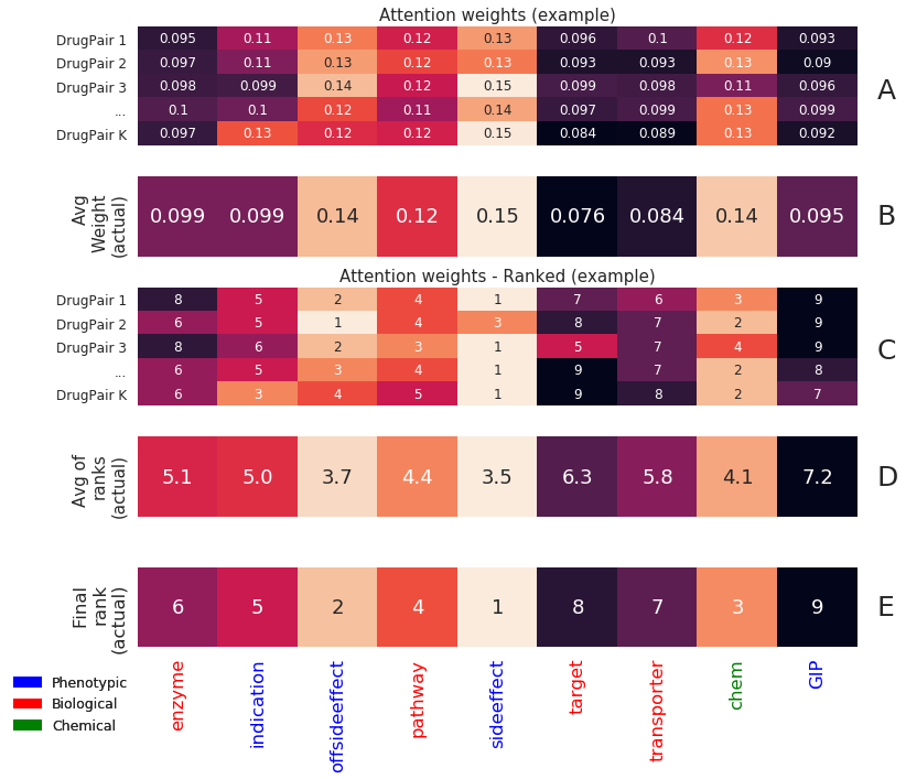
Figure 2: Feature Attention weights for DS1. A: Example weights for each drug pair. Each row represents the weights of the Feature Attention layer for each drug pair $(a,b)$ averaged. Since there are $K$ drug pairs in total and $9$ drug similarity matrices (columns) this is a $K\times 9$ matrix. The default value is $0.11(1/9)$ and each row sums to $1$. B: Average weights per column (similarity type) for the actual weights in the $K\times 9$ matrix from A. C: The absolute example weights for each row in A are ranked from highest ($1$) to lowest ($9$). D: Average ranks per column (similarity type) for the actual ranks in the $K\times 9$ matrix from C. E: The actual average values from D are ranked again to obtain the final similarity type rank from most important ($1$) to least important ($9$). Additionally, the similarity type labels were manually colored to indicate the level of information (phenotypic, biological, chemical).

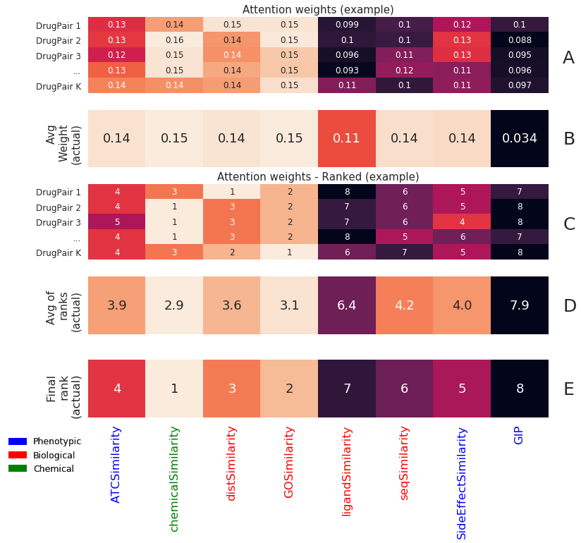
Figure 3: Feature Attention weights for DS3 with the CYP labels.

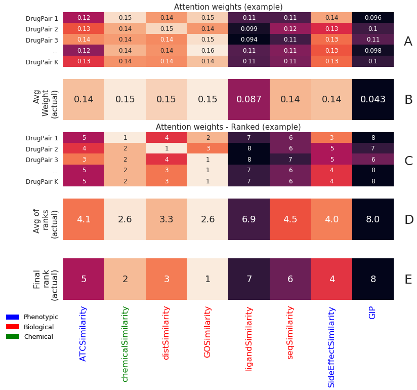
Figure 4: Feature Attention weights for DS3 with the NCYP labels.

Case Studies

To further test the efficiency of our model, we investigated the top predictions of our model through an external drug interaction database, DrugBank [17], which contains DDIs extracted from drug labels and scientific publications. We focused on the DS1 dataset, which links drug similarities to external drug IDs and therefore can be used for external validation. From DS1, we selected the top $20$ novel predictions ("false positives" according to the DS1 labels) with the highest interaction probabilities from our model, AttentionDDI. In Table 6 we list those drug pairs along with the interaction information from DrugBank. We found that $60\%$ of those top predictions were externally confirmed as known drug pair interactions.

Rank	ID A	ID B	Drug A	Drug B	Interaction
1	DB01194	DB00273	Brinzolamide	Topiramate	The risk or severity of adverse effects can be increased when Topiramate is combined with Brinzolamide.
2	DB01589	DB00678	Quazepam	Losartan	The metabolism of Quazepam can be decreased when combined with Losartan.
3	DB01212	DB00417	Ceftriaxone	PenicillinV	No interactions
4	DB01586	DB00951	Ursodeoxycholicacid	Isoniazid	No interactions
5	DB01337	DB00565	Pancuronium	Cisatracurium	Pancuronium may increase the central nervous system depressant (CNS depressant) activities of Cisatracurium.
6	DB00351	DB00484	Megestrolacetate	Brimonidine	No interactions
7	DB00530	DB00445	Erlotinib	Epirubicin	No interactions
8	DB00458	DB00659	Imipramine	Acamprosate	No interactions
9	DB01586	DB00319	Ursodeoxycholicacid	Piperacillin	No interactions
10	DB00443	DB00333	Betamethasone	Methadone	The metabolism of Methadone can be increased when combined with Betamethasone.
11	DB00458	DB00321	Imipramine	Amitriptyline	The metabolism of Amitriptyline can be decreased when combined with Imipramine.
12	DB00790	DB00584	Perindopril	Enalapril	The risk or severity of angioedema can be increased when Enalapril is combined with Perindopril.
13	DB01059	DB00448	Norfloxacin	Lansoprazole	No interactions
14	DB00571	DB01203	Propranolol	Nadolol	Propranolol may increase the arrhythmogenic activities of Nadolol.
15	DB00975	DB00627	Dipyridamole	Niacin	No interactions
16	DB00967	DB01173	Desloratadine	Orphenadrine	Desloratadine may increase the central nervous system depressant (CNS depressant) activities of Orphenadrine.
17	DB00222	DB00328	Glimepiride	Indomethacin	The protein binding of Glimepiride can be decreased when combined with Indomethacin.
18	DB00193	DB01183	Tramadol	Naloxone	The metabolism of Naloxone can be decreased when combined with Tramadol.
19	DB00904	DB00918	Ondansetron	Almotriptan	The risk or severity of adverse effects can be increased when Ondansetron is combined with Almotriptan.
20	DB00423	DB00794	Methocarbamol	Primidone	The risk or severity of adverse effects can be increased when Methocarbamol is combined with Primidone.

Table 6: Case studies for the top predictions in DS1. Interaction information from the DrugBank database.

Discussion

End-to-end solution

In this work, we presented an end-to-end architecture that utilizes attention mechanism to train a DDI prediction model. When looking at the DDI models reported in the literature, most of them consist of separate steps for model training. For example, the two competing baseline models (NDD and ISCMF) consist of multiple cascaded steps such as 1) matrix selection/filtering, 2) matrix fusion, and 3) classification that are optimized separately during model training. Preferably, the matrix selection would be informed by the classification goal which would optimize this selection. However, the first two steps (matrix filtering and fusion) are independent from classification and therefore not informed by the model training task. In contrast, our model uses a holistic approach in which all computational steps are connected and optimized while minimizing the loss function of our classifier. Consequently, our model is able to optimize the input information for DDI predictions at every computational step.

Explainability

Along with DDI predictions, our model makes it possible to gain additional information, which is the learned focus of the model on the input features. All similarity matrices are utilized as input data without being filtered. Hence, during training, the model learns which input information is more relevant for the classification task and weighs it accordingly. This is advantageous because the less relevant information is not completely discarded (as in the baseline model), but still taken into account as it may still provide some useful input for improved predictions.

Moreover, when looking at the relative importance (i.e., rank) of the attention weights, the phenotypic information such as drug side effect similarities were ranked higher than the lower level information (biological) in DS1 (Figure 2). This agrees with the conclusion in [18], as phenotypic information is considered more informative for DDI predictions while biological and chemical information might provide less translational power. In DS3 for both the CYP, as well as the NCYP labels, the similarity matrices were more evenly weighted (Figures 3 and 4) without showing a clear dominant information modality. Hence, we have shown the potential of applying Attention based models on multi-modal biological dataset (i.e., on drug similarity features like side effects, drug targets, chemical structure, etc.) by highlighting the input that is most relevant for DDI prediction.

Weighing the loss functions

Our model’s loss function was defined by a linear combination of two loss functions: (1) the negative log-likelihood loss (NLL) and (2) the contrastive loss (equation 16). The contribution of the NLL loss was included as a standardized loss used in classification tasks. On the other hand, the contrastive loss focuses on minimizing the intra-class distances (among positive or negative samples) and maximize the inter-class distances (between positive and negative samples).

In our experiments, the importance of contrastive loss over the NLL loss became evident especially for DS3 datasets. For DS1 and DS2, a uniform weight between both losses would result in similar performance as reported in the manuscript. However, biasing the weight towards contrastive loss (i.e., $95\%$ more importance for contrastive loss) helped increasing the performance by approximately 1 to 2 $\%$ for DS1 or DS2. However, for the DS3 dataset, weighing heavily (i.e., $95\%$) the contrastive loss was they key factor for achieving the high performance reported in the results section. This could be an indication that the positive and negative samples (that lead to drug interactions or not) are in close distance to each other and not well separated. In such a case, the contrastive loss would assist in better separating those samples and hence improve model performance. This was pronounced in the case of the DS3 dataset, where the proportions of positive samples are low ($\sim 1.5\%$ for CYP, $\sim 6\%$ for NCYP). Accordingly, the contrastive loss helped in the imbalanced label setting where the separability between classes is harder due to the low number of positive samples.

Conclusions

DDIs have important implications on patient treatment and safety. Due to the large number of possible drug pair combinations, many possible DDIs remain to be discovered. Thus, DDI prediction methods, and particularly computational methods, can aid in the accelerated discovery of additional interactions. These results are valuable for healthcare professionals that aim at finding the most effective treatment combinations while attempting to minimize unintended drug side effects.

In conclusion,, we present a novel DDI prediction solution which employs Attention, a mechanism that has successfully advanced model performance in other domains (such as NLP). We demonstrated that Attention based models can be successfully adapted to multi-modal biological data in the DDI domain with increased DDI prediction performance over various benchmark datasets and enhanced model explainability.

Availability of data and materials

The preprocessing scripts and the models’ implementation (training and testing) workflow is made publicly available at https://github.com/uzh-dqbm-cmi/side-effects/tree/attn_siamese_scheduler_clean

Competing interests

The authors declare that they have no competing interests.

Acknowledgements

NA.

Author’s contributions

KS and AA worked on the development of processing and analysis workflow, algorithms and models implementation. KS, AA, and NPG analyzed and interpreted the data. KS drafted the manuscript. NPG, AA, and MK supervised and edited the manuscript. All authors approved the final article.

Acronyms

ATC	Anatomical Therapeutic Chemical
CYP	Cytochrome P450
DDI	Drug-Drug Interaction
GIP	Gaussian Interaction Profile
GO	Gene Ontology
NLP	Natural Language Processing
PPI	Protein-Protein Interaction
SNF	Similarity Network Fusion
TP	True Positive
TN	True Negative
FP	False Positive
FN	False Negative
TPR	True Positive Rate
FPR	False Positive Rate
AUC	Area Under Curve
NLL	Negative Log-Likelihood
ROC	Receiver Operating Characteristic
PR	Precision-Recall

References

- [1] Kantor, E.D., Rehm, C.D., Haas, J.S., Chan, A.T., Giovannucci, E.L.: Trends in Prescription Drug Use Among Adults in the United States From 1999-2012. JAMA 314(17), 1818–1830 (2015). doi:10.1001/jama.2015.13766. Publisher: American Medical Association. Accessed 2020-08-10
- [2] Ryu, J.Y., Kim, H.U., Lee, S.Y.: Deep learning improves prediction of drug–drug and drug–food interactions. Proceedings of the National Academy of Sciences 115(18), 4304–4311 (2018). doi:10.1073/pnas.1803294115. Publisher: National Academy of Sciences Section: PNAS Plus. Accessed 2020-07-15
- [3] Ma, T., Shang, J., Xiao, C., Sun, J.: GENN: Predicting Correlated Drug-drug Interactions with Graph Energy Neural Networks. arXiv:1910.02107 [cs, q-bio, stat] (2019). arXiv: 1910.02107. Accessed 2020-07-15
- [4] Rohani, N., Eslahchi, C.: Drug-Drug Interaction Predicting by Neural Network Using Integrated Similarity. Scientific Reports 9(1), 13645 (2019). doi:10.1038/s41598-019-50121-3. Number: 1 Publisher: Nature Publishing Group. Accessed 2020-07-15
- [5] Rohani, N., Eslahchi, C., Katanforoush, A.: ISCMF: Integrated similarity-constrained matrix factorization for drug–drug interaction prediction. Network Modeling Analysis in Health Informatics and Bioinformatics 9(1), 11 (2020). doi:10.1007/s13721-019-0215-3. Accessed 2020-10-05
- [6] Vaswani, A., Shazeer, N., Parmar, N., Uszkoreit, J., Jones, L., Gomez, A.N., Kaiser, L., Polosukhin, I.: Attention is All you Need. In: Guyon, I., Luxburg, U.V., Bengio, S., Wallach, H., Fergus, R., Vishwanathan, S., Garnett, R. (eds.) Advances in Neural Information Processing Systems 30, pp. 5998–6008. Curran Associates, Inc., ??? (2017). http://papers.nips.cc/paper/7181-attention-is-all-you-need.pdf Accessed 2020-07-15
- [7] Zhang, W., Chen, Y., Liu, F., Luo, F., Tian, G., Li, X.: Predicting potential drug-drug interactions by integrating chemical, biological, phenotypic and network data. BMC Bioinformatics 18(1), 18 (2017). doi:10.1186/s12859-016-1415-9. Accessed 2020-07-15
- [8] Wan, F., Hong, L., Xiao, A., Jiang, T., Zeng, J.: NeoDTI: neural integration of neighbor information from a heterogeneous network for discovering new drug–target interactions. Bioinformatics 35(1), 104–111 (2019). doi:10.1093/bioinformatics/bty543. Publisher: Oxford Academic. Accessed 2020-07-15
- [9] Gottlieb, A., Stein, G.Y., Oron, Y., Ruppin, E., Sharan, R.: INDI: a computational framework for inferring drug interactions and their associated recommendations. Molecular Systems Biology 8(1), 592 (2012). doi:10.1038/msb.2012.26. Publisher: John Wiley & Sons, Ltd. Accessed 2020-07-15
- [10] van Laarhoven, T., Nabuurs, S.B., Marchiori, E.: Gaussian interaction profile kernels for predicting drug–target interaction. Bioinformatics 27(21), 3036–3043 (2011). doi:10.1093/bioinformatics/btr500. Publisher: Oxford Academic. Accessed 2020-09-23
- [11] Tatonetti, N.P., Ye, P.P., Daneshjou, R., Altman, R.B.: Data-Driven Prediction of Drug Effects and Interactions. Science Translational Medicine 4(125), 125–3112531 (2012). doi:10.1126/scitranslmed.3003377. Publisher: American Association for the Advancement of Science Section: Research Article. Accessed 2020-07-29
- [12] Wang, B., Mezlini, A.M., Demir, F., Fiume, M., Tu, Z., Brudno, M., Haibe-Kains, B., Goldenberg, A.: Similarity network fusion for aggregating data types on a genomic scale. Nature Methods 11(3), 333–337 (2014). doi:10.1038/nmeth.2810. Number: 3 Publisher: Nature Publishing Group. Accessed 2020-07-15
- [13] Paszke, A., Gross, S., Chintala, S., Chanan, G., Yang, E., DeVito, Z., Lin, Z., Desmaison, A., Antiga, L., Lerer, A.: Automatic differentiation in PyTorch (2017). Accessed 2020-07-29
- [14] Chicco, D.: In: Cartwright, H. (ed.) Siamese Neural Networks: An Overview, pp. 73–94. Springer, New York, NY (2021)
- [15] He, K., Zhang, X., Ren, S., Sun, J.: Deep residual learning for image recognition. In: Proceedings of the IEEE Computer Society Conference on Computer Vision and Pattern Recognition, vol. 2016-December, pp. 770–778. IEEE Computer Society, ??? (2016). doi:10.1109/CVPR.2016.90. 1512.03385
- [16] Ba, J.L., Kiros, J.R., Hinton, G.E.: Layer Normalization (2016). 1607.06450
- [17] Wishart, D.S., Feunang, Y.D., Guo, A.C., Lo, E.J., Marcu, A., Grant, J.R., Sajed, T., Johnson, D., Li, C., Sayeeda, Z., Assempour, N., Iynkkaran, I., Liu, Y., Maciejewski, A., Gale, N., Wilson, A., Chin, L., Cummings, R., Le, D., Pon, A., Knox, C., Wilson, M.: DrugBank 5.0: a major update to the DrugBank database for 2018. Nucleic Acids Research 46(D1), 1074–1082 (2018). doi:10.1093/nar/gkx1037. Accessed 2020-10-14
- [18] Zhang, P., Wang, F., Hu, J., Sorrentino, R.: Label Propagation Prediction of Drug-Drug Interactions Based on Clinical Side Effects. Scientific Reports 5(1), 1–10 (2015). doi:10.1038/srep12339. Accessed 2020-10-13