New constraints on the planetary system around the young active star AU Mic

AU Microscopii (AU Mic) is a young, active star whose transiting planet was recently detected. Here, we report our analysis of its TESS light curve, where we modeled the BY Draconis type quasi-periodic rotational modulation by starspots simultaneously to the flaring activity and planetary transits. We measured a flare occurrence rate in AU Mic of 6.35 flares per day for flares with amplitudes in the range of $0.06\%<f_{\rm max}<1.5\%$ of the star flux. We employed a Bayesian MCMC analysis to model the five transits of AU Mic b observed by TESS, improving the constraints on the planetary parameters. The measured planet-to-star effective radius ratio of $R_{\rm p}/R_{\star}=0.0496\pm 0.0007$ implies a physical radius of $4.07\pm 0.17$ R${}_{\Earth}$ and a planet density of $1.4\pm 0.4$ g cm${}^{-3}$, confirming that AU Mic b is a Neptune-size moderately inflated planet. While a single feature possibly due to a second planet was previously reported in the former TESS data, we report the detection of two additional transit-like events in the new TESS observations of July 2020. This represents substantial evidence for a second planet (AU Mic c) in the system. We analyzed its three available transits and obtained an orbital period of $18.859019\pm 0.000016$ d and a planetary radius of $3.24\pm 0.16$ R${}_{\Earth}$, which defines AU Mic c as a warm Neptune-size planet with an expected mass in the range of 2.2 M${}_{\Earth}$$<M_{\rm c}<$25.0 M${}_{\Earth}$, estimated from the population of exoplanets of similar sizes. The two planets in the AU Mic system are in near 9:4 mean-motion resonance. We show that this configuration is dynamically stable and should produce transit-timing variations (TTV). Our non-detection of significant TTV in AU Mic b suggests an upper limit for the mass of AU Mic c of $<7$ M${}_{\Earth}$, indicating that this planet is also likely to be inflated. As a young multi-planet system with at least two transiting planets, AU Mic becomes a key system for the study of atmospheres of infant planets and of planet-planet and planet-disk dynamics at the early stages of planetary evolution.

1 Introduction

Young planetary systems represent an opportunity to observe planets in the early stages of planetary formation when gravitational interactions have not significantly changed the initial configuration of the system. AU Microscopii (AU Mic) is a particularly interesting young system, with an estimated age of $22\pm 3$ Myr (mamjek2014), which is located at a distance of only $9.7248\pm 0.0046$ pc (gaiadr22018). Table 1 summarizes the star parameters of AU Mic that are relevant for this work. The AU Mic host is an M1 star with a spatially resolved edge-on debris disk (kalas2004) and at least one transiting planet, AU Mic b (plavchan2020Natur). This Neptune-size planet is in a $8.5$-d prograde orbit aligned with the stellar rotation axis (martioli2020; hirano2020; palle2020). While plavchan2020Natur only reported an upper limit on the mass of AU Mic b, klein2020 measured $17.1^{+4.7}_{-4.5}$M${}_{\Earth}$ thanks to infrared observations secured with the SPIRou spectropolarimeter (donati2020). plavchan2020Natur has also reported the detection of an isolated transit event of a second possible candidate planet, hereafter referred to as AU Mic c.

The notion that AU Mic could be a host for several planets is not a surprising one. Indeed, the occurrence rate of planets with a radius between 0.5 R${}_{\Earth}$ and 4.0 R${}_{\Earth}$ and a period between 0.5 and 256 d is estimated as $8.4^{+1.2}_{-1.1}$ planets per M dwarf (Hsu2020), although the occurrence rate of more massive planets in M dwarfs decreases significantly with mass (e.g., bonfils2013). Moreover, provided the fact that AU Mic has an edge-on debris disk and that AU Mic b is a transiting planet with an aligned orbit, the chances that other planets also reside in co-planar orbits increase and, therefore, possible close-in additional planets are also likely to transit the star.

AU Mic is a magnetically active star with strong flaring activity (Robinson2001). Its surface is largely filled by starspots, producing a BY Draconis-type light curve with a quasi-periodic rotational modulation and a period of $4.863\pm 0.010$ d (plavchan2020Natur). As in other active stars, the strong flaring and magnetic activity of AU Mic makes it more difficult to detect planetary transits in a photometric time series, especially for small planets where the occurrence rate is higher. In this work, we present an analysis of the Transiting Exoplanet Survey Satellite (TESS) data of AU Mic, including the new observations obtained in July 2020, where we implement a multi-flare model combined with the starspots model, improving the constraints on the planetary parameters from transit modeling and allowing for the detection of two additional transits of the second candidate planet AU Mic c.

Table 1: AU Mic star parameters.

Parameter	Value	Ref.
effective temperature	$3700\pm 100$ K	1
star mass	$0.50\pm 0.03$ M$\mathrm{{}_{\odot}}$	1
star radius	$0.75\pm 0.03$ R${}_{\odot}$	2
rotation period	$4.863\pm 0.010$ d	1
age	$22\pm 3$ Myr	3
distance	$9.7248\pm 0.0046$ parsec	4
linear limb dark. coef.	0.2348	5
quadratic limb dark. coef.	0.3750	5

(1) plavchan2020Natur; (2) russel2015; (3) mamjek2014; (4) gaiadr22018; (5) claret2018

2 TESS light curve

AU Mic was observed by TESS (tess_paper) in Sector 1 from 2018-Jul-25 to 2018-Aug-22, in cycle 1, camera 1. Then it was observed again in Sector 27 from 2020-Jul-04 to 2020-Jul-30, in cycle 3, camera 1. The second visit was observed as part of the TESS Guest Investigator Programs G03263 (PI: P. Plavchan), G03141 (PI: E. Newton), and G03273 (PI: L. Vega) in fast mode with a time sampling of 20 sec compared to the 2 min time sampling of the first visit. We obtained the de-trended photometric time series from the Mikulski Archive for Space Telescopes (MAST) using the MAST astroquery tool . Figure 1 shows the AU Mic PDCSAP flux in units of electrons-per-second (e${}^{-}$s${}^{-1}$) as a function of time given in TESS Barycentric Julian Date (TBJD = BJD - 2,457,000.0) for the two visits. plavchan2020Natur have analyzed the same TESS data from the first visit only, and in the present paper we report for the first time an analysis including the more recent 2020 TESS data. The predicted times of the transits of AU Mic b and c as calculated from our ephemerides (see Sects. 5 and 6) are marked with vertical lines.

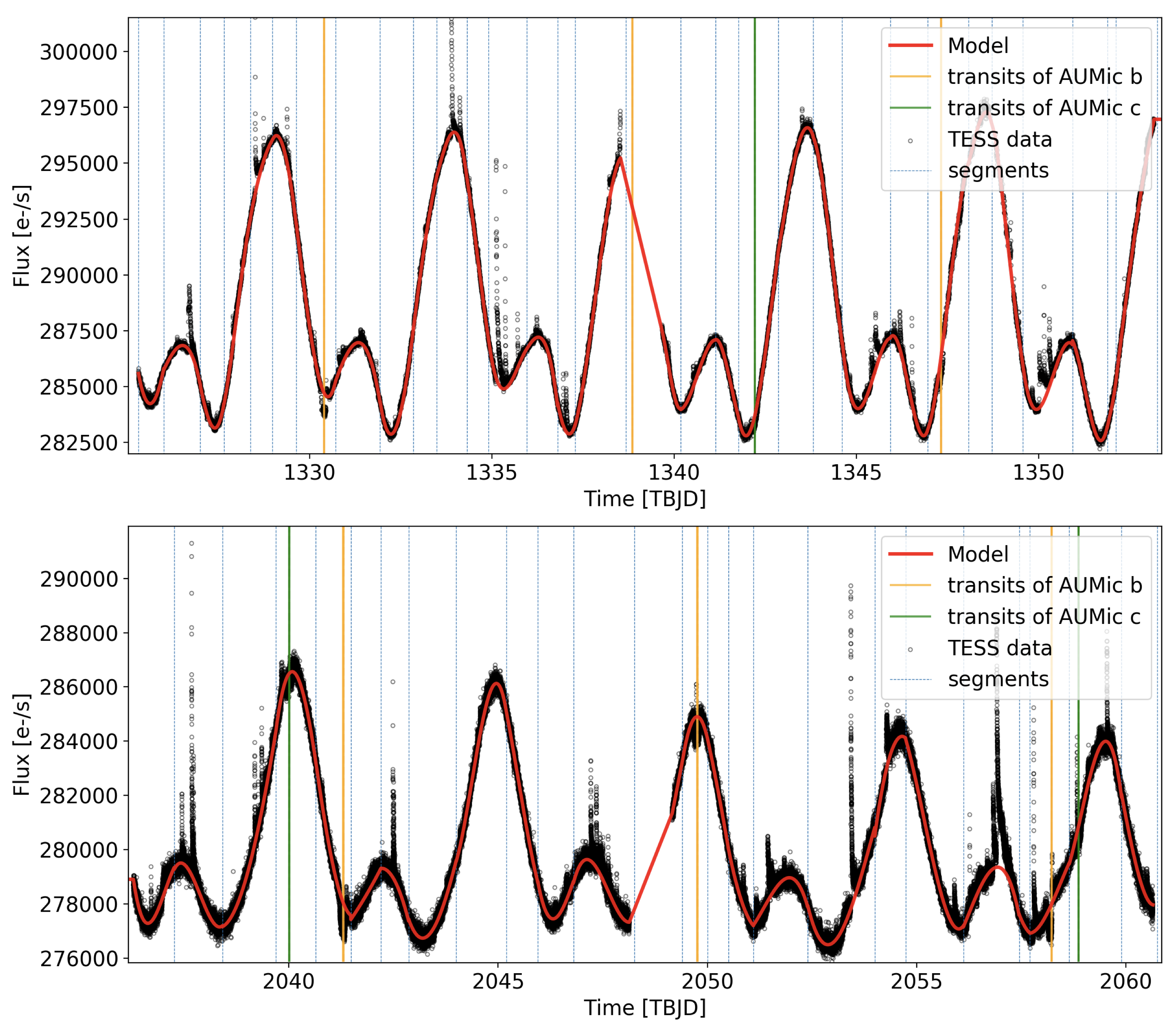
Figure 1: TESS light curve of AU Mic. Top panel: Data for the first visit (from 2018-Jul-25 to 2018-Aug-22). Bottom panel: Data for the second visit (from 2020-Jul-04 to 2020-Jul-30). Black points are the PDCSAP flux and vertical solid lines show the times of planetary transits, as obtained in our analysis, for AU Mic b (in orange) and AU Mic c (in green). Blue vertical dashed lines show the knots of selected ranges for the piece-wise polynomial fit and the red line shows the starspot model.

3 Starspots

As illustrated in Fig. 1, the TESS light curve of AU Mic shows a typical BY Draconis type of quasi-periodic variation due to starspots modulated by stellar rotation. The starspots evolve and, therefore, this modulation cannot be accurately modeled by a single periodic function. Thus, we treat this quasi-periodic modulation as a baseline “continuum” signal, where we model it by fitting a piece-wise fourth-order polynomial with iterative sigma-clipping. This approach works well when the ranges are carefully selected and inspected as follows. First, we can be certain that the polynomial function is a sufficiently accurate approximation for the local baseline variation within each range. Then we avoid the edges of the ranges to include either a transit or a flare event. Finally, we avoid the inclusion of large gaps (when TESS did not deliver data) within the same range. The edges for all selected ranges are represented by the blue vertical dashed lines in Fig. 1.

This starspot model is removed from the data to model flares and planetary transits as explained in Sects. 4, 5, and 6, which are further removed from the original data to fit the starspot modulation again. We repeat this procedure iteratively until the standard deviation of residuals is not improved by more than 1%. We typically meet this criterion upon three to five iterations. The final starspot model is also shown in Fig. 1. In Appendix LABEL:app:starrotation, we present an independent measurement of the rotational period of AU Mic from the starspot modulation in the 2018 TESS data.

4 Flares

AU Mic is an active young star with intense flaring activity. We carry out an analysis of the flares in the TESS data to improve the constraints on the transit events. We consider the starspot-subtracted residuals as shown in Fig. 2. The flares are typically clusters of points lying above the noise level. First we detect peaks as possible candidate flares using the scipy.signal.find_peaks routine, where it finds local maxima via a simple comparison of neighbouring values. We set a minimum peak amplitude of $2.5\sigma$ and a minimum horizontal distance between peaks of about $\sim 100$ minutes. Some flares in AU Mic are quite complex, while other flares occur before a previously initiated flare has ended. Therefore, we visually inspected all detected peaks to identify any possible additional peaks that have been missed by the find-peaks algorithm. After a few iterations, we identified a total of 324 flares in the whole TESS time series.

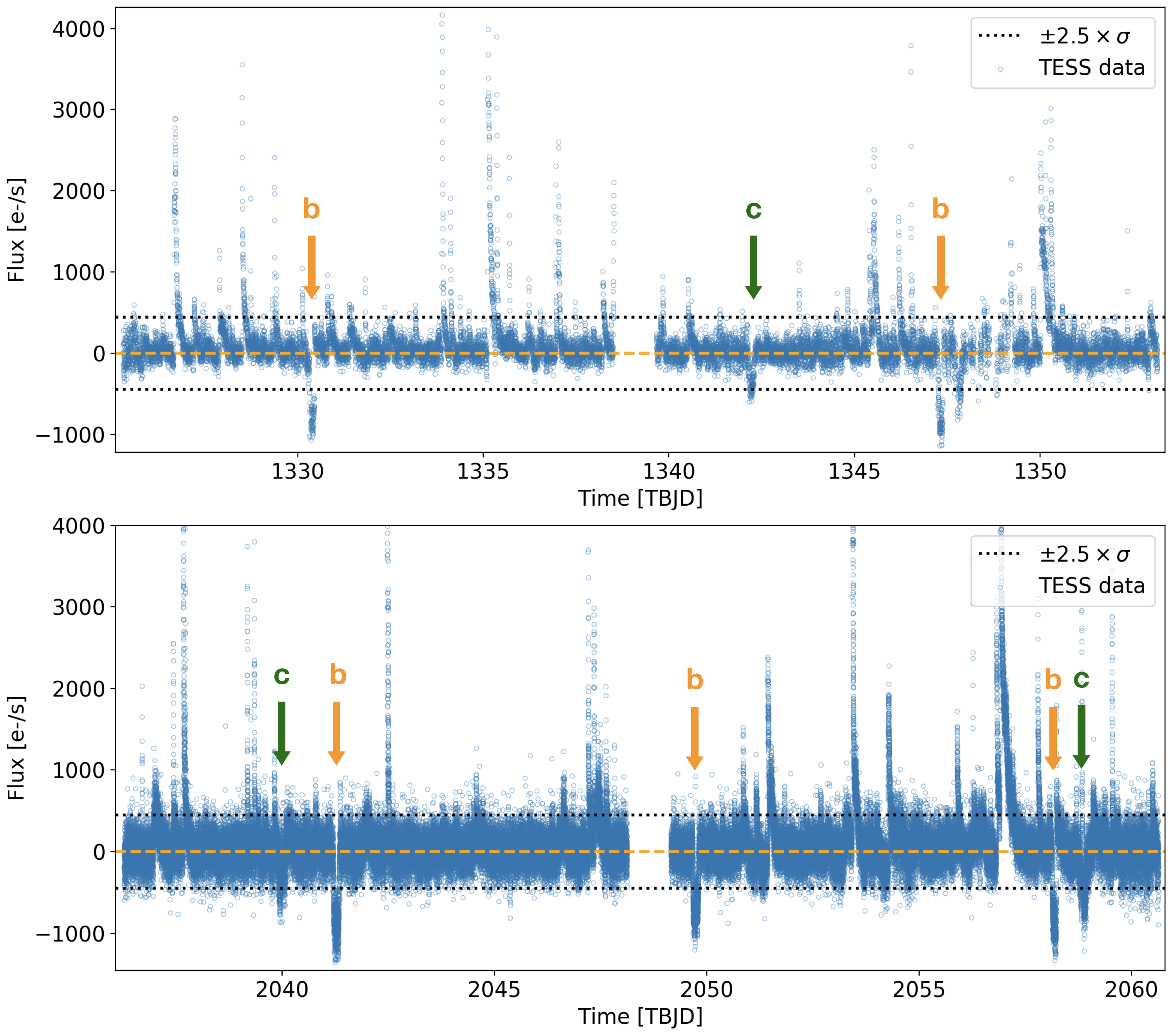
Figure 2: TESS residual light curve of AU Mic. Top panel: Residual light curve for the first TESS visit (2018-Jul-25 to 2018-Aug-22). Bottom panel: Residual curve for the second visit (2020-Jul-04 to 2020-Jul-30). Blue circles show AU Mic TESS flux data after subtracting the starspot model and black dotted lines show $\pm 2.5\sigma$ range around the starspot fit model, for $\sigma=162.5$ e${}^{-}$s${}^{-1}$. The flaring activity can be seen as positive groups of points above $+2.5\sigma$ and the transits as negative groups of points below $-2.5\sigma$. Our predicted times of transits for AU Mic b (in orange) and AU Mic c (in green) are marked with arrows.

The times and amplitudes of detected peaks were adopted as initial values for the basis of performing a least-squares fit using the multi-flare model of Davenport2014, where each flare is represented by a two-phase model with a polynomial rise and an exponential decay. Figure 3 shows, as an example, the residual light curve and fit flares model for three days of flaring activity in AU Mic in both TESS visits. For each flare in the model, we fit the flare amplitude ($f_{\rm max}$), the full width at half maximum (FWHM), and the time of maximum $t_{\rm peak}$. The fit parameters for all flares are presented in Appendix LABEL:app:flaresfitparams.

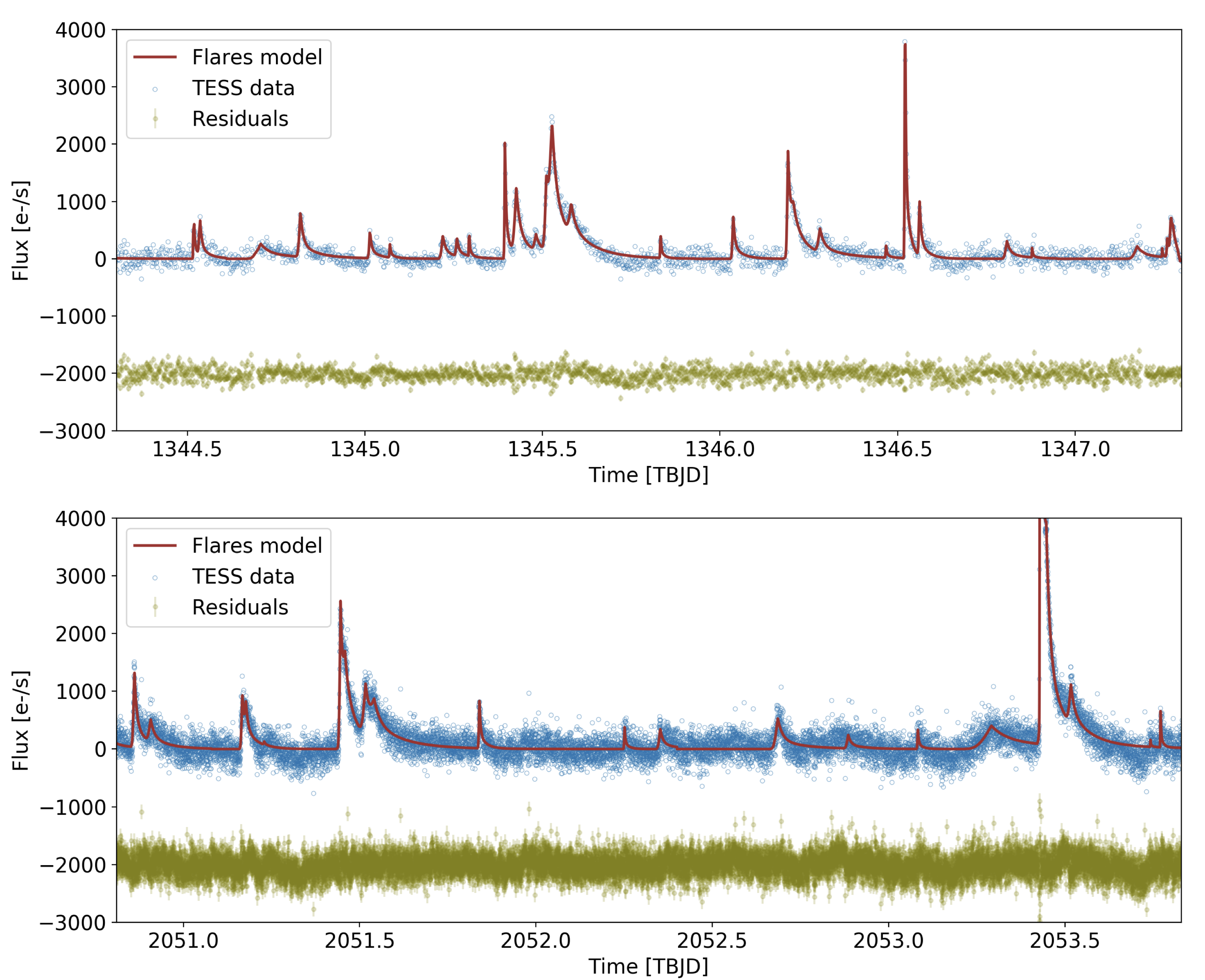
Figure 3: TESS residual light curve of AU Mic between TBJD=1344.3 and TBJD=1347.3 (top panel) and between TBJD=2050.8 and TBJD=2053.8 (bottom panel). Blue circles show the flux after subtracting the starspot model, brown line shows the multi-flare best fit model. Green points show the residuals with an arbitrary offset for better visualization. The dispersion of residuals are 107 e${}^{-}$s${}^{-1}$ and 178 e${}^{-}$s${}^{-1}$ for data presented in top panel and bottom panel, respectively.

The total continuous monitoring time of AU Mic performed by TESS was estimated as 49.75 d, where we have discounted the large gaps in the data. We detected a total of 324 flares, from which 316 have fit amplitudes above $F_{\rm max}>1\sigma$, for $\sigma=161.5$ e${}^{-}$s${}^{-1}$. Thus, the AU Mic global occurrence rate of flares with amplitude above $f_{\rm max}\gtrsim 0.06$% of the median stellar flux ($279544$ e${}^{-}$s${}^{-1}$) is estimated as 6.35 flares per day or about 1 flare every 3.8 hours. Figure 4 shows the distribution of flares as function of flare amplitudes. We fit an exponential to the measured distribution and obtained an empirical model for the occurrence rate as function of flare amplitude of $f_{r}=0.17{\rm e}^{-4.0f_{\rm max}}$ d${}^{-1}$, with $f_{\rm max}$ in units of $10^{2}$ e${}^{-}$s${}^{-1}$. We notice that the strong flares, which are more important energetically, have a much lower occurrence rate and therefore a low statistical significance in our analysis. Thus, this empirical relationship is only expected to hold for flares above the detection limit imposed by the noise and for flares with a statistically significant number of events observed in the TESS data, that is, those with amplitudes in the range of $0.06\%<f_{\rm max}<1.5\%$ of the star flux.

The transit duration of AU Mic b calculated by plavchan2020Natur is about 3.5 hours with transit depth of 0.26%. Therefore, considering that a transit observation of AU Mic b requires an out-of-transit baseline of about 2 hours, it is most likely that any transit observation in AU Mic should be affected in some way by flare events. This shows the importance of modeling flares adequately to improve the constraints on the planetary parameters obtained by the transits.

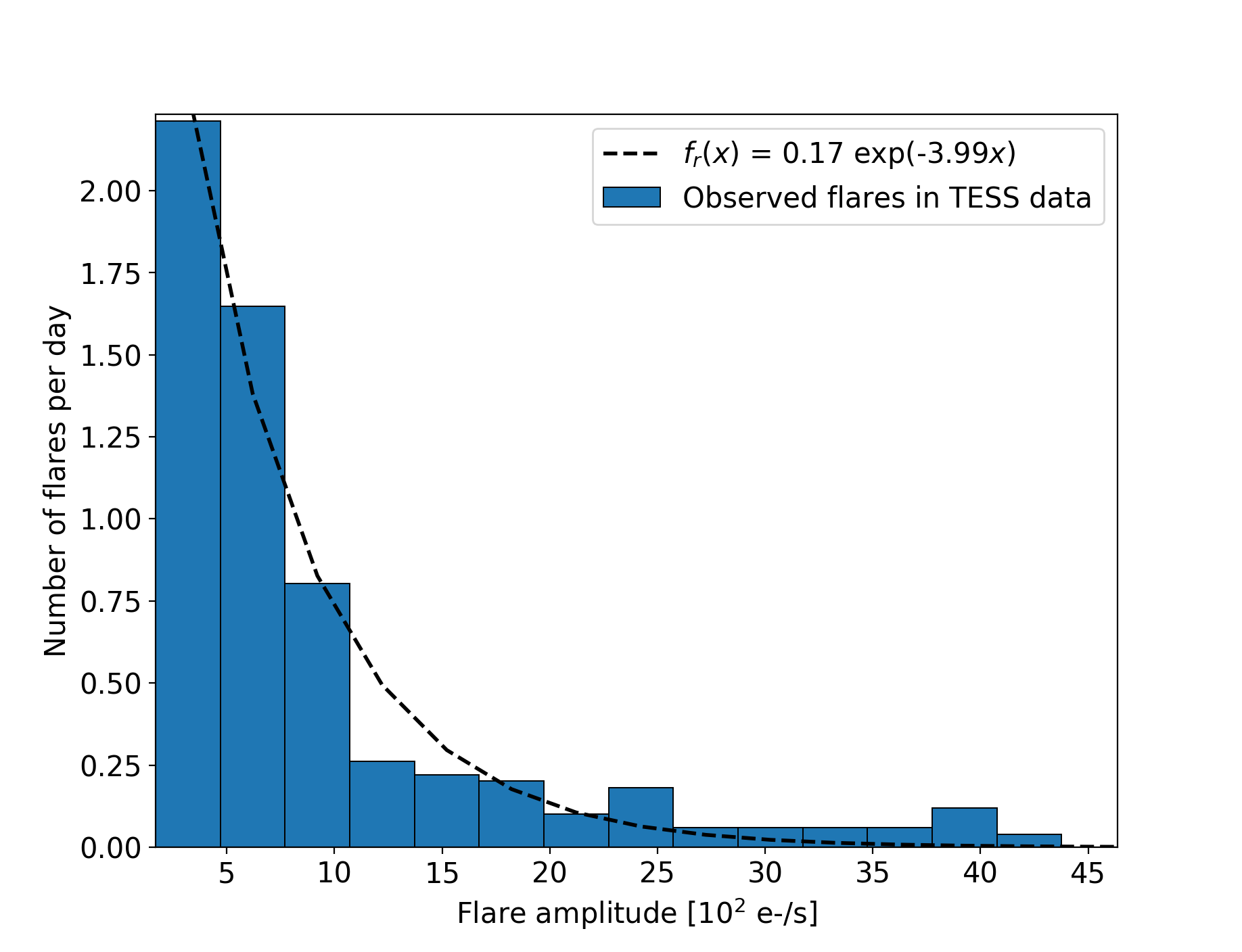
Figure 4: Number of flares normalized by the total observed time of 49.75 d as function of flare amplitude. Dashed line shows the fit to an exponential decay as shown in the legend, where variable $x$ represents the flare amplitude.

5 Transits of AU Mic b

Three transits of AU Mic b occurred during the first TESS visit, but only two have been observed due to a communication problem with the spacecraft during the second transit (see plavchan2020Natur). For the second visit, three other transits were expected, and indeed we were able to identify all of them. To analyze these five transits together, we start with the parameters of AU Mic b from plavchan2020Natur, referred to as ”prior values” in Table 2, to remove the transit signal from the TESS light curve before fitting the starspot and flare models. Our transit model is calculated using the BATMAN toolkit by Kreidberg2015, where we assume a circular orbit ($e=0$). This assumption is in agreement with plavchan2020Natur, who did not detect any significant eccentricity from their analysis of the transits only, where the eccentricity would be slightly constrained by the duration of the transit. We adopt as priors the quadratic limb-darkening coefficients (LDC) from claret2018 with an arbitrary error of 0.1, where we obtained the values calculated for the photometric system of TESS and those matching the closest stellar parameters to those of AU Mic (see Table 1).

The transits of AU Mic b, flares, and starspots are fit simultaneously using the non-linear least squares optimization (OLS) fit tool scipy.optimize.leastsq. As explained in Sect. 3 this procedure is run iteratively, where we first obtain an independent fit for each component of the model and then we set these values as initial guess to run an OLS analysis with all free parameters in the three components of the model. Then we consider the data in the ranges around the transits of AU Mic b to sample the posterior distributions of the transit parameters using the emcee Markov chain Monte Carlo (MCMC) package (foreman2013). The chain is set with 100 walkers and 30000 MCMC steps of which we discard the first 5000. The MCMC samples are presented in Fig. LABEL:fig:aumic_b_mcmc_chain in Appendix LABEL:app:posteriordistributions, which show the chains reaching stability before the first 5000 discarded steps. The posterior distributions are illustrated in Fig. LABEL:fig:aumic_b_pairsplot in Appendix LABEL:app:posteriordistributions. The best-fit values of the transit parameters are calculated as the medians of the posterior distribution with error bars defined by the 34% on each side of the median, all presented in Table 2.

Figure 5 shows the results of our analysis for each transit range separately, and the bottom right panel shows the flux normalized by the starspot and flare models for all transits together, and our best fit model along with the previous model of plavchan2020Natur for comparison. The dispersion of residuals are 358, 433, 633, 566, and 588 ppm, for each respective epoch. The global dispersion is 573 ppm. Notice that our measured parameters of AU Mic b agree within $3\sigma$ with the previous measurements by plavchan2020Natur but with improved accuracy. Our measured planet-to-star radius ratio is slightly larger than that measured by plavchan2020Natur (see lower, right panel of Fig. 5). However, as described in Sect. 7, our derived effective planetary radius of $1.05\pm 0.04$ R${}_{\mathrm{Nep}}$ is slightly smaller than the value $1.08\pm 0.05$ R${}_{\mathrm{Nep}}$ reported by plavchan2020Natur.

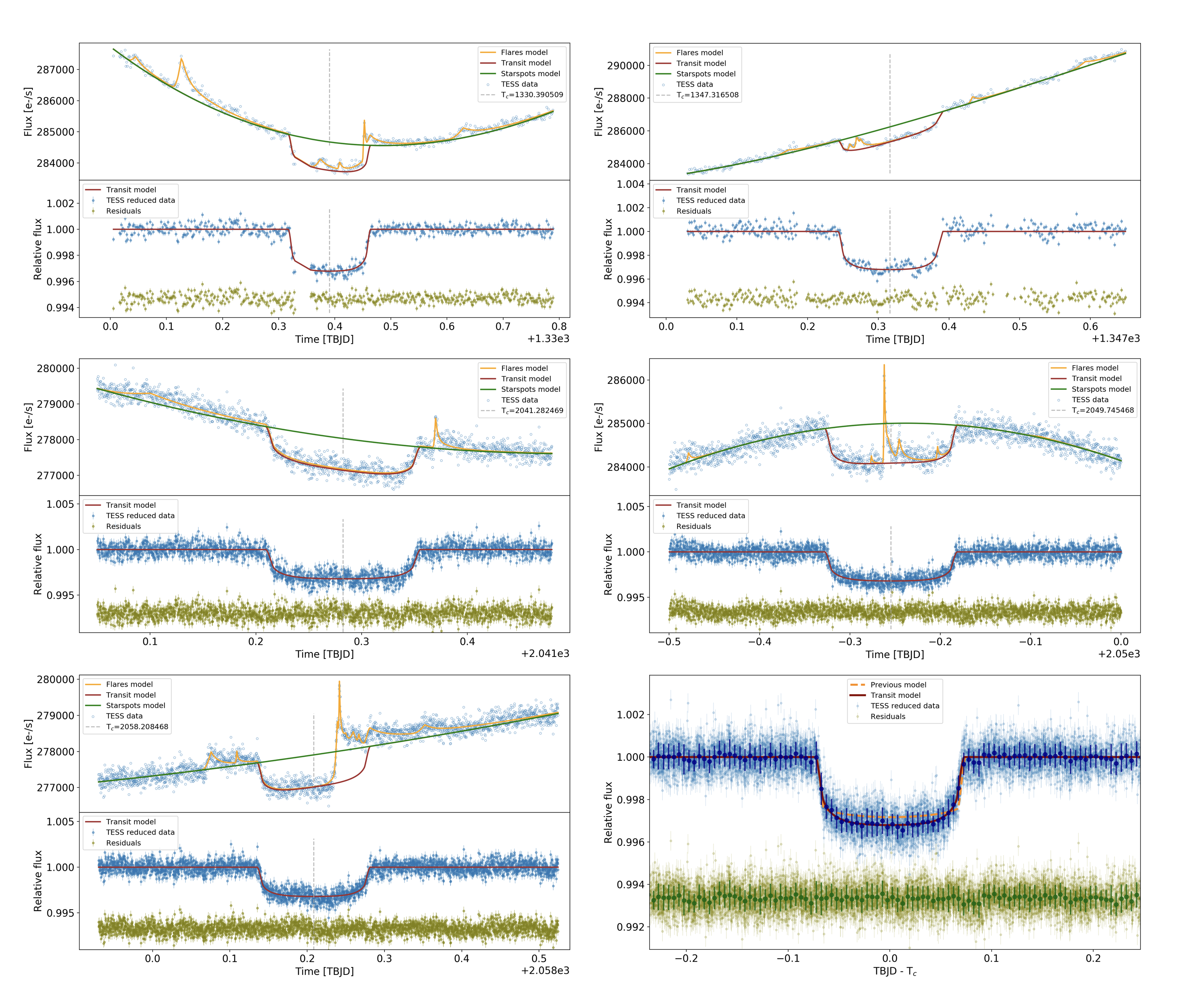
Figure 5: Each panel shows the range around one of the five transits of AU Mic b observed by TESS. The top part of each panel shows the TESS data (blue circles) and the best-fit model for each component, as indicated in the legend. The bottom part in each panel shows the TESS data normalized by the starspot and flare model (blue points) and the best-fit transit model (red line). Vertical dashed lines show the central time of each transit. The bottom right panel shows the phase-folded light curve for all the data from the five transits (light blue points) and the binned data (dark blue points) with a bin size of 0.005 d, our best fit model (red line), and the previous fit model of plavchan2020Natur for comparison (orange dashed line). The residuals (green points) are displayed with an arbitrary offset.

Table 2: Transit fit parameters for planet AU Mic b obtained in our analysis from a simultaneous fit of the five transits observed by TESS as illustrated in Figs. 5 and LABEL:fig:aumic_b_pairsplot.

Parameter	Prior value	MCMC fit value
time of conjunction, $T_{0}$ [TBJD]	$1330.38957^{+0.00015}_{-0.00068}$	$1330.39051\pm 0.00015$
orbital period, $P$ [d]	$8.46321\pm 0.00004$	$8.463000\pm 0.000002$
normalized semi-major axis, $a/R_{\star}$	$19.1^{+1.8}_{-1.6}$	$19.1^{+0.2}_{-0.4}$
orbital inclination, $i$ [degree]	$89.5^{\pm}0.4$	$89.5^{+0.4}_{-0.3}$
planet-to-star radius ratio, $R_{\rm p}/R_{\star}$	$0.0514\pm 0.0013$	$0.0526^{+0.0003}_{-0.0002}$
linear limb dark. coef., $u_{0}$	$\mathcal{N}(0.23,0.1)$	$0.13\pm 0.03$
quadratic limb dark. coef., $u_{1}$	$\mathcal{N}(0.38,0.1)$	$0.58\pm 0.06$

6 Confirmation and characterization of planet AU Mic c

An isolated candidate transit event at $T_{c}=1342.22\pm 0.03$ TBJD was identified in the 2018 TESS data by plavchan2020Natur, which was interpreted as a possible second planet in a $30\pm 6$-d orbit. We have searched for other transit-like events in the TESS data by looking at regions with systematic flux dips below the noise level. We identified three regions as potential transits including the one previously identified by plavchan2020Natur (see Fig. 2). We notice that there is an additional region presenting a significant flux dip around ${\rm TBJD}=1347.8$, which did not include as a possible transit. The 2018 TESS data after ${\rm TBJD}\sim 1347.7$ contain several gaps, which have an impact on the modeling of the baseline modulation by starspots as well as on the detection and modeling of flares. Therefore, we presume that the apparent flux dip in this region is more likely due to a misfit other than a transit. In addition the shape of that dip is different from that of the three features above.

We hypothesize that the three selected events are transits of the same candidate planet AU Mic c. In order to test this hypothesis, we first obtain an orbital period that is consistent with the three transits, that is, a period given by the slope of a linear fit to the ephemeris equation, $T_{c}=T_{0}+P\times E$, with $T_{c}$ as the times of conjunction measured independently for each event and $E$ as the corresponding epochs to each event, assumed to be 0, 37, and 38. We find an orbital period of $P=18.85895\pm 0.00003$ d. However, we note that with this particular periodicity, only three events would occur during the TESS observations (see Fig. 1). The possibility of shorter alias periods is ruled out by the fact that TESS would have observed more transits of this object and we did not detect them. To test further our hypothesis, we performed an independent analysis of each event assuming an orbital period, first with an uniform prior of $P=\mathcal{U}(1,500)$ d to explore a broad range of periods, and then with a normal prior of $P=\mathcal{N}(18.86,0.01)$ d, which explores a solution constrained by the previous knowledge imposed by our hypothesis. Analogously, the normalized semi-major axes are also first set with an uniform prior of $a/R_{\star}=\mathcal{U}(1,500)$ and then with a normal prior estimated using the Kepler’s law, that is, $a/R_{\star}=\mathcal{N}(31.5,1.4)$. The priors for the times of conjunction are measured locally on each event, for example, for the first event, we obtained $T_{0}=\mathcal{N}(1342.23,0.01)$. The prior for the planet-to-star radius ratio is estimated from the square root of the average flux depth of the three events, assuming a conservative error, that is, $R_{\rm p}/R_{\star}=\mathcal{N}(0.04,0.01)$. The orbital inclination is considered with an uniform prior distribution of $i=\mathcal{U}(85^{\circ},90^{\circ})$ and the limb darkening coefficients are fixed to the literature values presented in Table 1. In Appendix LABEL:app:individualtransitsofaumicc, we present the results for this independent analysis of each transit. The posterior of all the transit parameters agree within $3\sigma$ (see Table LABEL:tab:othertransitsfitparams), and the dispersion of residuals improves when we adopted the fit period of $P=\mathcal{N}(18.86,0.01)$ d as prior, which supports our hypothesis that these three events were caused by the transits of the same planet AU Mic c. Finally, we perform a joint analysis of the three transits simultaneously, where we adopt the same priors as in the independent analysis above, except for the limb darkening coefficients, where we adopted a normal prior with the literature values and an arbitrary error of 1.0. We call attention to the fact that the limb darkening coefficients obtained in Sect. 5 could have been used as priors since both planets are transiting the same star. However, the two planets may transit the stellar disk in different regions, and since AU Mic is largely filled by starspots, the limb darkening may also be affected by the different temperatures of the transited regions in the photosphere. Table 3 presents the priors and fit parameters, while Fig. 6 shows the TESS data for the three transits and the best-fit model obtained from our analysis. As in Sect. 5, the MCMC samples and posterior distributions are illustrated in Figs. LABEL:fig:aumic_c_mcmc_chain and LABEL:fig:aumic_c_pairsplot in Appendix LABEL:app:posteriordistributions.

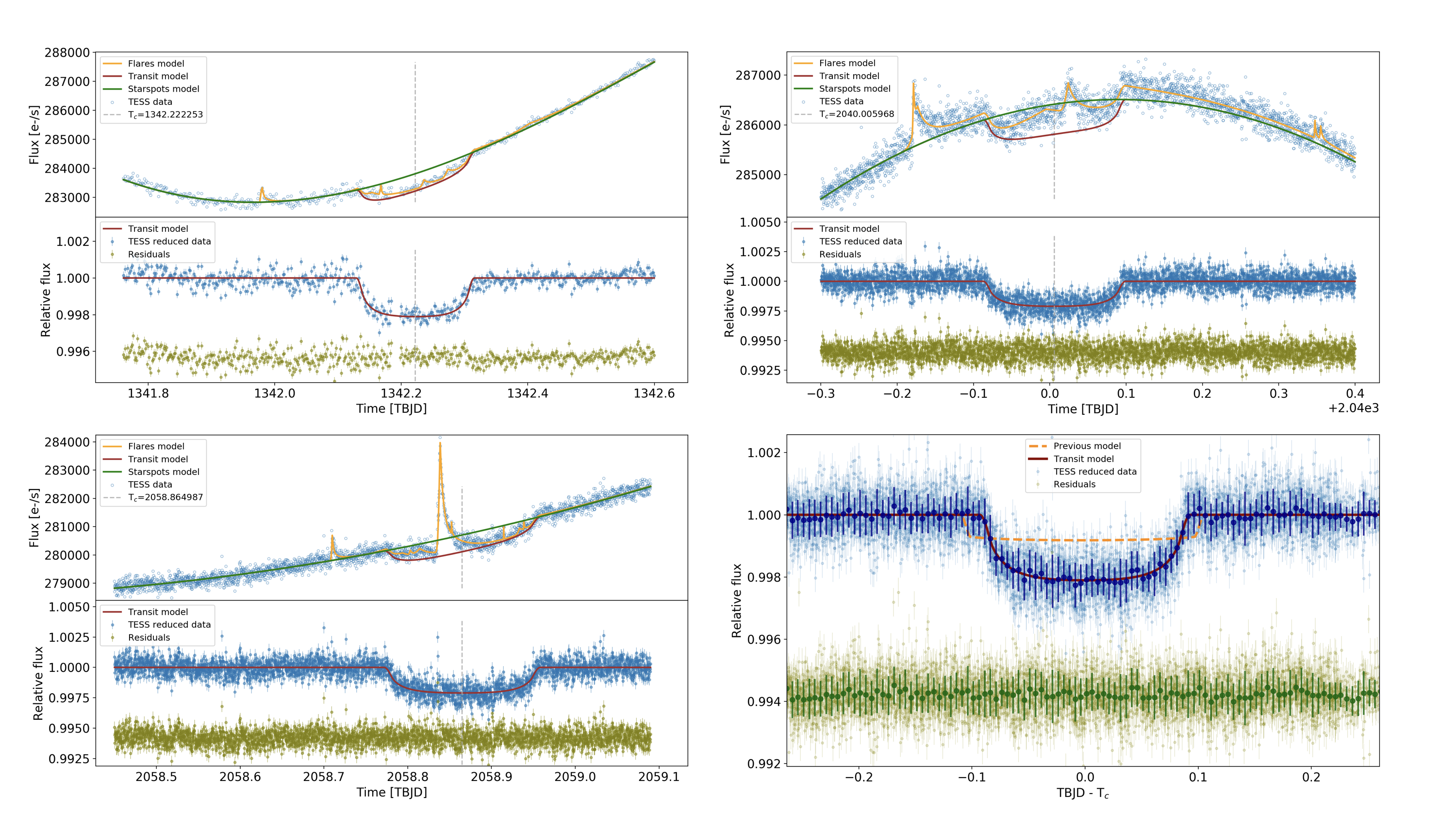
Figure 6: Each panel shows the range around one of the five transits of AU Mic b observed by TESS. Details are the same as in Fig. 5, but here we present the results for the three TESS transits of AU Mic c. The dispersion of residuals are 370, 646, 609 ppm, for each respective epoch. The global dispersion is 609 ppm.

Table 3: Transit fit parameters for planet AU Mic c obtained in our analysis from a simultaneous fit of the three transits observed by TESS as illustrated in Figs. 6 and LABEL:fig:aumic_c_pairsplot.

Parameter	Prior value	MCMC fit value
time of conjunction, $T_{0}$ [TBJD]	$\mathcal{N}(1342.23,0.01)$	$1342.2223\pm 0.0005$
orbital period, $P$ [d]	$\mathcal{N}(18.86,0.01)$	$18.859019^{+0.000016}_{-0.000015}$
normalized semi-major axis, $a/R_{\star}$	$\mathcal{N}(31.5,1.4)$	$29\pm 3$
orbital inclination, $i$ [degree]	$\mathcal{U}(85,90)$	$89.0^{+0.5}_{-0.4}$
planet-to-star radius ratio, $R_{\rm p}/R_{\star}$	$\mathcal{N}(0.04,0.01)$	$0.0418^{+0.0010}_{-0.0012}$
linear limb dark. coef., $u_{0}$	$\mathcal{N}(0.23,1.0)$	$0.0^{+0.2}_{-0.3}$
quadratic limb dark. coef., $u_{1}$	$\mathcal{N}(0.38,1.0)$	$1.2^{+0.4}_{-0.3}$

7 Discussion

We combine the transit parameters of AU Mic b and c presented in Tables 2 and 3 with the star parameters from Table 1 to calculate a number of derived parameters, which are presented in Table 4.

Table 4: Summary of the parameters of planets AU Mic b and AU Mic c.

Parameter	unit	AU Mic b	AU Mic c
time of conjunction	TBJD	$1330.39051\pm 0.00015$	$1342.2223\pm 0.0005$
orbital period	d	$8.463000\pm 0.000002$	$18.859019\pm 0.000016$
normalized semi-major axis, $a/R_{\star}$	-	$19.1\pm 0.3$	$29\pm 3$
semi-major axis ${}^{\dagger}$	au	$0.0645\pm 0.0013$	$0.1101\pm 0.0022$
transit duration	h	$3.50\pm 0.08$	$4.5\pm 0.8$
orbital inclination	degree	$89.5\pm 0.3$	$89.0^{+0.5}_{-0.4}$
impact parameter	$R_{\star}$	$0.18\pm 0.11$	$0.51\pm 0.21$
eccentricity	-	$0$ (FIXED)	$0$ (FIXED)
planet-to-star radius ratio ${}^{\S}$, $R_{p}/R_{\star}$	-	$0.0496\pm 0.0007$	$0.0395\pm 0.0011$
planet radius	R${}_{\mathrm{Jup}}$	$0.371\pm 0.016$	$0.295\pm 0.014$
planet radius	R${}_{\mathrm{Nep}}$	$1.05\pm 0.04$	$0.84\pm 0.04$
planet radius	R${}_{\Earth}$	$4.07\pm 0.17$	$3.24\pm 0.16$
velocity semi-amplitude	m s${}^{-1}$	$8.5^{+2.3}_{-2.2}$ ${}^{\S\S}$	$0.8<K_{\rm c}<9.5$
planet mass	M${}_{\mathrm{Jup}}$	$0.054\pm 0.015$ ${}^{\S\S}$	0.007 ¡ M${}_{\rm c}$ ¡ 0.079
planet mass	M${}_{\mathrm{Nep}}$	$1.00\pm 0.27$ ${}^{\S\S}$	0.13 ¡ M${}_{\rm c}$ ¡ 1.46
planet mass	M${}_{\Earth}$	$17\pm 5$ ${}^{\S\S}$	2.2 ¡ M${}_{\rm c}$ ¡ 25.0
planet density	g cm${}^{-3}$	$1.4\pm 0.4$	$0.4<\rho_{\rm c}<4.1$
equilibrium temperature	K	$593\pm 21$	$454\pm 16$

${}^{\dagger}$ semi-major axis derived from the fit period and the Kepler’s law; ${}^{\S}$ radius values correspond to the effective radius, which is already corrected for spot coverage and contains an additional uncertainty due to rotational modulation, as explained in Sect. 7; ${}^{\S\S}$ klein2020