Memory-Efficient Hierarchical Neural Architecture Search for Image Restoration

Abstract

Recently, much attention has been spent on neural architecture search (NAS), aiming to outperform those manually-designed neural architectures on high-level vision recognition tasks. Inspired by the success, here we attempt to leverage NAS techniques to automatically design efficient network architectures for low-level image restoration tasks. In particular, we propose a memory-efficient hierarchical NAS (termed HiNAS) and apply it to two such tasks: image denoising and image super-resolution. HiNAS adopts gradient based search strategies and builds a flexible hierarchical search space, including the inner search space and outer search space. They are in charge of designing cell architectures and deciding cell widths, respectively. For the inner search space, we propose a layer-wise architecture sharing strategy (LWAS), resulting in more flexible architectures and better performance. For the outer search space, we design a cell-sharing strategy to save memory, and considerably accelerate the search speed. The proposed HiNAS method is both memory and computation efficient. With a single GTX1080Ti GPU, it takes only about 1 hour for searching for denoising network on the BSD-500 dataset and 3.5 hours for searching for the super-resolution structure on the DIV2K dataset. Experiments show that the architectures found by HiNAS have fewer parameters and enjoy a faster inference speed, while achieving highly competitive performance compared with state-of-the-art methods. Code is available at:

https://github.com/hkzhang91/HiNAS

1 Introduction

As a classical task in computer vision, image restoration aims to estimate the underlying image from its degraded measurements, which is known as an ill-posed inverse procedure. Depending on the type of degradation, image restoration can be categorized into various sub-problems, e.g., denoising, super-resolution, deblur, dehaze, and inpainting, etc. In this work, we focus on image denoising and image super-resolution.

Image denoising aims to restore a clean image from a noisy one. Owing to the fact that noise corruption always occurs in the image sensing process and inevitably degrades the visual quality of collected images, image denoising is needed for various computer vision tasks (Chatterjee and Milanfar, 2009). The purpose of single image super-resolution is to estimate a higher-resolution image from a low-resolution one. In early days, single image super-resolution methods mainly are based on interpolation, such as nearest-neighbor, bilinear and bicubic. These simple methods are computationally very efficient, but do not yield satisfactory results. Recent methods on image denoising and image super-resolution have shifted their approaches to deep learning, which build a mapping function from low-quality images to the desired corresponding high-quality images using convolutional networks or Transformers, and have often outperformed conventional methods significantly (Mao et al., 2016; Tai et al., 2017; Tobias Plötz, 2018; Liu et al., 2019d; Dong et al., 2015; Zhang et al., 2018c, e; Dai et al., 2019). To date, most of these methods focus on improving the quality of the restored images, and largely neglect the inference speed. As such, these image restoration models typically contain millions or even tens of millions of parameters. Some methods involve a recurrent optimization process to improve restoration quality, resulting in slow inference speed. Effort has been spent on employing compact models for faster inference. However, it is not trivial to manually design compact models that enjoy both good accuracy and a fast inference speed.

Recently, a growing interest is witnessed in developing solutions to automate the manual process of architecture design. Architectures automatically found by algorithms have achieved highly competitive performance in high-level vision tasks such as image classification (Zoph and Le, 2017), object detection (Ghiasi et al., 2019; Wang et al., 2020) and semantic segmentation (Liu et al., 2019a; Nekrasov et al., 2019). Very recently, several works on using NAS algorithms to design architectures for image restoration have been proposed. For instance, FALSR (Chu et al., 2019a), E-CAE (Suganuma et al., 2018) and EvoNet (Liu et al., 2019c). Compared with the manually designed architectures, the architectures found by NAS algorithms achieve higher performance and/or have fewer parameters. A drawback is that the search process of these methods are very computationally demanding. By using four Tesla V100 GPUs, the method of E-CAE needs 44 hours on searching. FALSR takes about 3 days on 8 Tesla V100 GPUs to find promising architectures.

In summary, deep learning based image restoration methods show promising performances, but designing an efficient architecture requires substantial efforts. Current NAS based image restoration approaches overcome the problem of designing architectures, but introduce a new problem—these methods require a relatively large number of computing resources. In addition, most of these methods do not pay attention to the inference speed, which is very important in practice. In this paper, we attempt to solve these problems by designing a memory-efficient NAS algorithm. Specifically, we propose a memory-efficient NAS algorithm. The proposed NAS algorithm can automatically search for neural architectures efficiently for low-level image processing tasks, which solves the problem of designing architectures requiring substantial efforts. As the proposed is memory-efficient, it does not need a significant amount of computing resources. In addition, we also take the inference speed into consideration.

In (Zhang et al., 2020), we have used deformable convolution to build the search space, as it is more flexible and powerful than conventional convolutions. The searched results also prove that deformable convolution is very useful in improving performance. However, we later find that deformable convolutions can be more time-consuming than standard convolutions. Thus, in this paper, deformable convolution is abandoned to improve the inference speed. Unfortunately, although abandoning deformable convolution does improve the inference speed, it leads to lower accuracy. To fill this gap, we design a new search space, by proposing a layer-wise architecture sharing strategy and adopting the residual learning structure. Benefiting from this, the architectures founded by our method here enjoys a faster inference speed, while achieving good performance.

We demonstrate the effectiveness of our method on two image processing applications, namely image denoising and image super-resolution. Our main contributions can be summarized as follows.

1. Built upon gradient based NAS algorithms, here we propose a memory- and computation-efficient hierarchical neural architecture search approach for image denoising and image super-resolution, termed HiNAS. To our knowledge, this may be the first attempt to apply differentiable architecture search algorithms to low-level vision tasks.

2. We propose a layer-wise architecture sharing strategy to improve the flexibility of the search space and propose cell sharing to save memory. Both strategies contribute to the efficiency of the proposed HiNAS, which only takes hours to search for architectures for image restoration tasks with a single GTX 1080Ti GPU.

3. We apply HiNAS to image denoising with various noise modes, and image super-resolution for evaluation. Experiments show that the networks found by our HiNAS achieves highly competitive performance compared with state-of-the-art algorithms, while having fewer parameters and faster inference speed.

4. We conduct experiments to analyze the network architectures found by our NAS algorithm in terms of the internal structure, offering some insights in architectures found by NAS.

We review some relevant work next.

2 Related Work

2.1 Image Denoising and Super-resolution

Currently, due to the popularity of convolutional neural networks (CNNs), image restoration algorithms including image denoising and image super-resolution achieved a significant performance boost. For image denoising, the notable network models, DnCNN (Zhang et al., 2017a) and IrCNN (Zhang et al., 2017b), predict the residue, instead of the denoised image. FFDNet (Zhang et al., 2018b) attempts to address spatially varying noise by appending noise level maps to the input of DnCNN. NLRN (Liu et al., 2018a) incorporates non-local operations into a recurrent neural network (RNN) for image restoration. N3Net (Tobias Plötz, 2018) formulates a differentiable version of nearest neighbor search to further improve DnCNN.

Recently, some algorithms focus on using real-world noisy-clean image pairs to train the deep denoising model. Previously, almost all such models are trained using synthetic noisy-clean image pairs, and there is a risk of overfitting the model to the synthetic data. Along this line, CBDNet (Guo et al., 2019) uses a simulated camera pipeline to generate more realistic training data. Similar work in (Jaroensri et al., 2019) proposes a camera simulator that aims to accurately simulate the degradation and noise transformation performed by the image sensing pipeline of a camera.

For image super-resolution, the first attempt was proposed in (Dong et al., 2015), where Dong et al.  built a CNN model which consists of three convolutional layers. Compared with traditional approaches, this neural network model achieved impressive performance. Later, consistent with the development of CNN for other vision tasks, CNN based super-resolution approaches tend to employ deeper models. For instance, Kim et al. proposed VDSR (Kim et al., 2016a) and DRCN (Kim et al., 2016b). Both VDSR and DRCN contain 20 convolutional layers and employ the residual learning strategy. To address the issue of lacking of long-term memory (one state is usually influenced by a specific prior state). Tai et al.  (Tai et al., 2017) designed a memory block based on the recursive unit and gate unit, then built a MemNet by stacking the proposed block and connect them with skip connections.

In addition to designing deeper networks to improve accuracy, a few methods take spatial correlations into consideration and researchers attempt to embed the attention mechanism in their networks. For example, NLRN (Liu et al., 2018a) incorporates non-local modules in a recurrent network. Based on SENet (Hu et al., 2018), Zhang et al.  (Zhang et al., 2018d) built a very deep residual channel attention network for super-resolution. Recently, Dai et al.  (Dai et al., 2019) further extended the first-order channel attention to second-order channel attention. Liu et al.  (Liu et al., 2020) group several residual modules together via skip connections to aggregate features.

Apart from the image restoration quality, inference efficiency is critically important for image restoration tasks. Image restoration algorithms which can restore high-quality images from low-quality images in real time would be highly valuable. Based on light-weight network design, Ahn et al.  (Ahn et al., 2018) proposed a cascading residual network and Hui et al. (Hui et al., 2019) combined light-weight designing with information distillation. Very recently, Lee et al. (Lee et al., 2020) boost the inference speed of FSRCNN (Hui et al., 2018) by using knowledge distillation. There is typically a trade-off between the accuracy and inference speed.

2.2 Network Architecture Search (NAS)

NAS aims to design automated approaches for discovering high-performance neural architectures such that the procedure of tedious and heuristic manual design of neural architectures can be largely eliminated from the pipeline.

As the optimization objective of NAS is very complex and in general non-differentiable, early approaches often employ evolutionary algorithms (EA) for optimizing the neural architectures and parameters. The best architecture may be obtained by iteratively mutating a population of candidate architectures (Liu et al., 2018b). An alternative to EA is to use reinforcement learning (RL) techniques, e.g., policy gradient (Zoph et al., 2018; Wang et al., 2020) and Q-learning (Zhong et al., 2018). With RL, one trains a recurrent neural network that acts as a meta-controller to generate potential architectures—typically encoded as sequences—by exploring a predefined search space. Note that EA and RL based methods suffer from a common drawback—inefficient search—often requiring a large amount of computation, as these methods can be viewed as zero-order optimization.

Speed-up techniques are therefore proposed to remedy this issue. Exemplar works include hyper-networks (Zhang et al., 2018a), network morphism (Elsken et al., 2018) and shared weights (Pham et al., 2018). Recently, an increasing number of NAS methods search for architecture via (first-order) gradient-based optimization (Liu et al., 2019b; Cai et al., 2019; Liu et al., 2019a). They relax the architecture representation as a supernet via continuous relaxation, then optimize architecture parameters of this supernet via gradient descent. Here, our proposed method adopts gradient-based search strategy.

Besides search strategies, how to design the search space is also very important for NAS algorithms. The search space defines which architectures can be represented. Early NAS approaches employ a very complex space of chain-structured search space. This chain-structured search space can be represented as a sequence of $n$ layers, each of which has different candidate operations, including different choices of convolution operations (depth-wise separable convolutions, dilated convolution) and pooling operations, where convolution operations can have different hyperparameters (the number of kernels, kernel sizes, and strides). Conducting architecture search on such a complex search space is computationally expensive, as the search space covers a wide range of architectures. For instance, Zoph and Le (2017) use a few hundred GPUs and take several days to carry out architecture search experiments on Cifar-10. Later, motivated by the fact that hand-crafted architectures usually consist of repeated modules, He et al. (2016) and Zoph et al. (2018) proposed the cell-structure search space. Different from the chain-structured search space where the overall architecture is searched directly, the cell-structure search space searches for an architectural building block and then construct the whole network by stacking the building block following a pre-designed outline structure. Thus, compared with the chain-structured search space, the cell-structured search space offers two major advantages: 1) the cell-structured search space covers a part of the model as cells, which consists of fewer layers, resulting in a much faster search speed. By adopting the cell-structured search space, Zoph et al. (2018) achieve a speed-up of 7$\times$ compared with (Zoph and Le, 2017); 2) The found architectures can be more easily transferred to other datasets by increasing or reducing the number of cells. Therefore, the cell-structured search space gradually gains popularity in recent works (Cai et al., 2018; Pham et al., 2018; Zhong et al., 2018; Liu et al., 2019b).

The search space of our proposed method integrates both the chain-structured search space and cell-structured space, by proposing a layer-wise architecture strategy. In previous works, the search algorithm only searches for a single cell and then constructs the overall network by stacking this cell repeatedly. Different layers have the same architecture, which sacrifices some flexibility. In this paper, for a network consisting of a sequence of $L$ cells, the proposed search algorithm searches for $L$ different cells. Designing different architectures for different layers is more flexible, and this design idea is consistent with that in Inception series (Szegedy et al., 2015, 2016, 2017). Benefiting from the fact that our search algorithm is gradient based, designing different architectures for different layers does not introduce any additional computational cost but $L-1$ sets of continuous variables. In other words, the proposed method enjoys the fast search speed of the cell-structured search space on the one hand, and has a more flexible “chain-structured-like” search space on the other hand.

Our work is most closely related to DARTS (Liu et al., 2019b), ProxylessNAS (Cai et al., 2019), DenseNAS (Fang et al., 2020), and Auto-Deeplab (Liu et al., 2019a). All these methods take the architecture searching process as an optimization process. They first build a supernet, which consists of all possible layer types and the corresponding weight parameters as the search space. Then they optimize the parameters of this supernet via gradient descent. Finally, they derive the final architecture according to weight parameters. DARTS firstly proposed the continuous relaxation of the architecture representation, allowing the efficient search of the cell architecture using gradient descent, which has achieved competitive performance. Motivated by this search efficiency, following DARTS and its successors, HiNAS also employs the gradient-based approach as its search strategy. Different from DARTS, the later four NAS algorithms include the kernel widths into their search space. In addition, the later four NAS algorithms discard the operation of searching for reduction cells. For ProxylessNAS, DenseNAS and Auto-Deeplab, the adjustment of spatial resolution is integrated into their candidate operations. For HiNAS, both the reduction cell and pooling operations are discarded to retain the high resolution of feature maps. The adjustment of the receptive field relies on selecting operations of different receptive fields. ProxylessNAS discovers sequential structures and chooses kernel widths within manually designed blocks (Inverted Bottlenecks (He et al., 2016)). DenseNAS extends the chain-structured search space and inserts more blocks of various widths at each stage. Each block is densely connected to its subsequent ones.

Different from ProxylessNAS and DenseNAS, the main body of HiNAS is cell-structured and the final structure is cell-based. Both Auto-Deeplab and HiNAS are designed for dense prediction tasks. By introducing multiple paths of different widths, Auto-Deeplab extends its search space by including kernel widths. The search space of our proposed HiNAS resembles Auto-Deeplab. The three main differences are as follows.

• For candidate operations, we discard pooling operations to retain the high resolution of feature maps and rely on automatically selected operations of different receptive fields to adapt the receptive field;

• We propose a layer-wise architecture-sharing strategy to improve flexibility;

• A cell-sharing strategy is proposed for improving memory efficiency.

Relevant to using NAS algorithms to search for neural network architectures for low-level image restoration tasks, three most related works are EvoNet (Liu et al., 2019c), E-CAE (Suganuma et al., 2018) and FALSR (Chu et al., 2019a). EvoNet searches for networks for medical image denoising via EA. E-CAE (Suganuma et al., 2018) employs EA to search for an architecture of convolutional auto-encoders for image inpainting and denoising. FALSR was proposed for image super-resolution tasks. FALSR combines RL and EA and designs a hybrid controller as its model generator. All three methods mentioned above require a relatively large amount of computations and take a large amount of GPU time for searching. Compared with these methods, our proposed HiNAS employs a different search space, and search strategies, leading to significantly higher search efficiency.

We now present our method in detail.

3 Our Method

Our proposed HiNAS is a gradient-based architecture search algorithm. Specifically, we search for $L$ different computation cells, where $L$ denotes the number of cells. The final architecture is built by stacking the $L$ cells of different widths one by one. To be able to search for both cell topological architectures and cell widths, HiNAS builds a hierarchical search space. The inner space is responsible for searching for the inner cell topological architectures, and the outer space is in charge of searching for cell widths. To further improve the efficiency of HiNAS, we propose a cell-sharing strategy, allowing features from different levels of the outer search space to share one cell.

In this section, we first introduce how to search for architectures of cells based on continuous relaxation (inner search space). Then we explain how to determine the widths via multiple candidate paths and cell sharing (outer search space). Then, we elaborate on residual learning frameworks for image denoising and super-resolution. Last, we present our search strategy and details of the loss functions.

3.1 Inner Search Space

Figure 1: Inner-cell architecture search. Left: the supercell that contains all possible layer types. Right: the cell architecture searching result, a compact cell, where each node only keeps the two most important inputs and each input is connected to the current node with a selected operation.

Figure 2: The overall framework of the supernet. The supernet contains three components, including the ‘start part’, ‘middle part’, and ‘end part’. The start and end parts are manually pre-designed and their architectures are fixed during search. The middle part is automatically found by the search algorithm. It consists of $L$ layers, each of which contains three cells of different widths. In the proposed HiNAS, cells in the same layer share the same architecture and cells in different layers can have different architectures. This improves the flexibility of the search space, resulting in better performance, while introducing no computation overhead. During search, all paths are activated, and the weight $\beta$ is updated via gradient descent. At the end of search, each layer keeps only one path, which is marked in a black arrow.

To search for the inner cell architecture, we first build a super-cell containing $N$ nodes. Different nodes in this supercell are connected with different paths, and each path contains all possible operations. Each operation in each path corresponds to a weight $\alpha$, which denotes the importance of this layer type in the current path. The purpose of the cell architecture search is to learn a set of continuous variables $\{\alpha\}$. During search, continuous variables are updated via gradient descent optimization. At the end of the search, a discrete architecture can be obtained by keeping the top two most probable layer types and discarding the rest for each node. Next, we explain this process in detail.

Shared inner-cell architecture search. We denote the supercell in layer $l$ as ${C}_{l}$, which takes outputs of previous cells and the cell before previous cells as inputs and outputs a tensor ${h}_{l}$, as shown in Figure 1. The left-side is the supercell containing all possible operations. It is a directed acyclic graph consists of three nodes. Inside ${C}_{l}$, each node takes the two inputs of the current cell and the outputs of all previous nodes as input and outputs a tensor ${h}_{l}$. When all layers share the same cell architecture, the output of the $i$th node in the cell is calculated as:

$$\begin{split}{}&{x}_{l,i}=\sum_{{x}_{j}\in{I}_{l,i}}{{O}^{j\rightarrow i}({x}_{j})},\\ {}&{O}^{j\rightarrow i}({x}_{j})=\sum_{k=1}^{S}{{{\alpha}_{k}^{j\rightarrow i}}{o}^{k}}({x}_{j}),\end{split}$$ (1)

where ${I}_{l,i}=\{{h}_{l-1},{h}_{l-2},{x}_{l,j<i}\}$ is the input set of node $i$. ${h}_{l-1}$ and ${h}_{l-2}$ are the outputs of cells in layers $l-1$ and $l-2$, respectively. ${O}_{l}^{j\rightarrow i}$ is the set of possible layer types. $\{{o}^{1},{o}^{2},\cdots,{o}^{S}\}$ correspond to $S$ possible operations. ${\alpha}_{k}^{j\rightarrow i}$ denotes the weight of operator ${o}^{k}$.

Layer-wise architecture sharing (LWAS). In fact, in early days, NAS methods often employ a very complex search space to search for the entire network directly, requiring an enormous number of GPUs and taking a significant amount of computation. For instance, Zoph et al. used a few hundred GPUs and train for several days to search for architectures on the small dataset of Cifar-10 (Zoph and Le, 2017). Later, Zoph et al.  proposed the NASNet, which searches for an architectural building block then build the overall network by stacking the found block with a pre-designed outline structure (Zoph et al., 2018). Compared with the method in (Zoph and Le, 2017), NASNet enjoys a much faster search speed. Thus, the search space design of NASNet is widely used in most recent works. NASNet significantly reduces the complexity of the search space, which is very useful for improving the search speed in RL and EA based NAS algorithms. Reducing the complexity of search space means training fewer student networks. The NASNet search space accelerates the search speed on one hand, with the price of restricting the flexibility of the search space. It restricts different layers of networks to share the same cell architecture. In our proposed HiNAS, we adopt a more flexible search space: we search for different cell architectures, for different layers. In our gradient based HiNAS, we only need to introduce more continuous variables ${\alpha}$ without any additional computational cost. In our new search space, the output of the $i$-th node is computed with:

$$\begin{split}{}&{x}_{l,i}=\sum_{{x}_{j}\in{I}_{l,i}}{{O}_{l}^{j\rightarrow i}({x}_{j})},\\ {}&{O}_{l}^{j\rightarrow i}({x}_{j})=\sum_{k=1}^{S}{{{\alpha}_{l}^{k,j\rightarrow i}}{o}^{k}}({x}_{j}).\end{split}$$ (2)

Here, ${\alpha}_{l}^{k,j\rightarrow i}$ is $l$ related. The sets of continuous variables ${\alpha}$ in different layers are different. Cells in the same layer share the same set of continuous variables ${\alpha}$. ${h}_{l}$ is the concatenation of the outputs of $N$ nodes, and it can be expressed as:

$$\begin{split}{h}_{l}={}&{\rm Cell}({h}_{l-1},{h}_{l-2})\\ ={}&{\rm Concat}\{{x}_{l,i}|i\in\{1,2,\cdots,N\}\}.\end{split}$$ (3)

Search space. In this paper, we employ the following 7 types of operators:

• conv: $3\times 3$ convolution;

• sep: $3\times 3$ separable convolution;

• sep: $5\times 5$ separable convolution;

• dil: $3\times 3$ convolution with dilation rate of 2;

• dil: $5\times 5$ convolution with dilation rate of 2;

• skip: skip connection;

• none: no connection and return zero.

To preserve pixel-level information for low-level image processing, we abandon down-sample operations such as pooling layers; and set the stride to 2 in convolution layers. For convolution operators, we employ three convolution types including standard convolutions, separable convolutions and dilation convolutions. Each convolution operator, in order, consists of a LeakyReLU activation layer, a convolution layer and a batch normalization layer. We provide two different kernel sizes of 3 and 5 for separable and dilation convolutions. The search algorithm can adapt the receptive field by selecting convolution operators of different kernel sizes. An example of found compact cell is shown in the right-side of Figure 1.

Figure 3: Comparison of cases of whether using cell sharing or not. Left: features from different levels share the same cell. Using cell sharing; Right: features from different levels use different cells.

3.2 Outer Search Space

Now, the main idea of searching for specific architectures inside cells has been presented. Beside search architectures of inner cells, we still need to either heuristically set the width of each cell or automatically search for a proper width for each cell, in order to build the overall network.

Multiple candidate paths. In conventional CNNs, the change of widths of convolution layers is often related to the change of spatial resolutions. For instance, once the features are down-sampled, the widths of following convolution layers are doubled. In our HiNAS, instead of using down-sample operations such as pooling layers and setting the stride to 2 in convolution layers, we rely on operations with different receptive field such as dilation convolution operations of $3\times 3$ and $5\times 5$, and separable convolution operations of $3\times 3$ and $5\times 5$ to adjust the receptive field automatically.

Thus, the conventional experience of adjusting width no longer applies to our case. To solve this problem, we employ the flexible hierarchical search space and leave the task of deciding the width of each cell to the NAS algorithm itself, making the search space more general. In fact, several NAS algorithms in the literature also search for the outer layer width, mostly for high-level image understanding tasks. For example, FBNet (Wu et al., 2019) and MNASNet (Tan et al., 2019) consider different expansion rates inside their modules to discover compact networks for image classification.

In this section, we introduce the outer layer width search space, which determines the widths of cells in different layers. Similarly, we build a supernet that contains several supercells with different widths in each layer. As illustrated in Figure 2, the supernet mainly consists of three parts:

1. ‘start-part’, consisting of an input layer and two convolution layers. A relatively shallow feature is extracted by feeding the input data to two convolution layers, and a copy of input data is propagated to the ‘end-part’ via skip connections;

2. ‘middle-part’, containing $L$ layers and each layer having three supercells of different widths. This is the main part of supernet. The shallow feature extracted in the ‘start-part’ is fed to different cells of layer $0$. Then the outputs of layer $0$ are fed to different cells of layer $1$, and so on;

3. ‘end-part’, concatenating the outputs of layer $L-1$, then feeding them to two convolution layers to generate the residual, finally element-wise summing the learned residual and the output of skip connection to obtain the final result.

Except layer $0$, which contains two cells of different widths, our supernet provides three paths of cells with different widths, which correspond to three decisions: 1) reducing the width; 2) keeping the previous width; 3) increasing the width. After searching, only one cell at each layer is kept. The continuous relaxation strategy mentioned in the cell architecture search section is reused here.

At each layer $l$, there are three cells ${C}_{l}^{0}$, ${C}_{l}^{1}$ and ${C}_{l}^{2}$ with widths ${\gamma}^{0}\times W$, ${\gamma}^{1}\times W$ and ${\gamma}^{2}\times W$, where $W$ is the basic width and ${\gamma}^{0}$, ${\gamma}^{1}$ and ${\gamma}^{2}$ are width changing factors. The output feature of each layer is

$${h}_{l}=\{{h}_{l}^{0},{h}_{l}^{1},{h}_{l}^{2}\},$$ (4)

where ${h}_{l}^{i}$ is the output of ${C}_{l}^{i}$. The channel width of ${h}_{l}^{i}$ is ${2}^{i}NW$, where $N$ is the number of nodes in the cells.

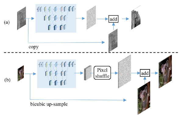
Figure 4: Residual learning frameworks. (a) residual learning framework for denoising; (b) residual learning framework for super-resolution.

Cell sharing. Each cell $C_{l}^{i}$ is connected to $C_{l-1}^{i-1}$, $C_{l-1}^{i}$ and $C_{l-1}^{i+1}$ in the previous layer and $C_{l-2}^{i}$ two layers before. We first process the outputs $h_{l-1}$ from those layers with a $1\times 1$ convolution to form features $f_{l-1}$ with width $2^{i}W$, matching the input of $C_{l}^{i}$. Then the output for the $i$th cell in layer $l$ is computed with

$${h}_{l}^{i}=C_{l}^{i}\left(\sum_{k=i-1}^{i+1}{\beta}_{k}^{i}{f}_{l-1}^{k},{f}_{l-2}^{i}\right),$$ (5)

where ${\beta}_{k}^{i}$ is the weight of ${f}_{l-1}^{k}$. We combine the three outputs of ${C}_{l-1}$ according to corresponding weights, then feed them to ${C}_{l}^{i}$ as input. Here, features ${f}_{l-1}^{i-1}$, ${f}_{l-1}^{i}$ and ${f}_{l-1}^{i+1}$ come from different levels, but they share the cell ${C}_{l}^{i}$ during computing ${h}_{l}^{i}$.

Note the similarity of this design with that of Auto-Deeplab, which is used to select feature strides for image segmentation. However, in Auto-Deeplab, the outputs from the three different levels are first processed by separate cells with different sets of weights before summing into the output:

$${h}_{l}^{i}=\sum_{k=i-1}^{i+1}{\beta}_{k}^{i}C_{l}^{k}({f}_{l-1}^{k},{f}_{l-2}^{i}),$$ (6)

A comparison between Eqs. (5) and (6) is shown in Figure 3, where the inputs from layer $l-1$ are not shown for simplicity.

For the hierarchical structure which has three candidate paths, the cell in each candidate path is used once with Eq. (5) and it is used for three times with Eq. (6). By sharing the cell $C_{l}^{i}$, we are able to save the memory consumption by a factor of 3 in the supernet. Cell sharing has two main advantages: 1) Improving applicability. NAS in general consumes much memory and computation. Improving memory efficiency enables much broader applications. 2) Improving searching efficiency. As cell sharing saves memory consumption in the supernet, during search, we can use larger batch sizes speed up the convergence and search speed. It also enables the use of a deeper and wider supernet for more accurate approximations.

As memory efficiency is important for NAS methods, some previous methods have already been proposed for better efficiency (Pham et al., 2018; Dong and Yang, 2019c; Cai et al., 2019; Dong and Yang, 2019b; Guo et al., 2020). Compared with memory-efficient strategies adopted in these methods, our proposed cell sharing strategy differs in the core idea. For ENAS (Pham et al., 2018), the core idea is loading pretrained weight into new the generated student networks to reduce the time cost of training from scratch. GDAS (Dong and Yang, 2019c), Proxyless-NAS (Cai et al., 2019), SETN (Dong and Yang, 2019b) and Single Path One-Shot NAS (Guo et al., 2020) share the same key idea, which is to avoid traversing all the possible operations during search. In PC-DARTS (Xu et al., 2021), for training the superent, a subset of channels of each path are activated in each iteration. The core idea of our cell sharing is reducing duplicate operations, processing the sum of outputs of different candidate paths rather than processing each output separately. A similar idea is also adopted in a concurrent work (Chen et al., 2019), the key idea of which is calculating the weighted sum of kernels rather than the output features.

Outer layer widths search appears to be an extension of the inner cell search. However, the way to obtain the final widths of different layers is different from that of obtaining the final compact cell architecture in the inner cell architecture search. If we follow previous actions as in the inner cell search, the widths of adjacent layers in the final network may change drastically, which would have a negative impact on the efficiency, as explained in (Ma et al., 2018). To avoid this problem, we view the $\beta$ values as a probability. Then use the Viterbi decoding algorithm to select the path with the maximum probability as the final result.

Different from these methods targeting the classification task, our search space considers the interaction between multi-level features with different receptive fields, so as to preserve high resolutions. To simultaneously consider hierarchical routing and inner cell design choices for width and operation, we build a multi-level supernet, of which every subnet can encode more powerful multi-level features than those single path networks.

There are several previous algorithms which also include width in their search space. AMC (He et al., 2018), FBNetV2 (Wan et al., 2020) and TuNAS (Bender et al., 2020) all assign different widths to different operations within a sequential search space. It is worth noting that our search space is essentially different from theirs, where operation-wise width search is not trivial. In addition, FBNetV2 searches for widths via channel masking. TAS (Dong and Yang, 2019a) prunes channels according to a learnable distribution, then transfers knowledge from the unpruned network to the pruned network via knowledge distillation. Both methods do not consider topology in their search space, thus being less flexible than ours.

Residual learning In our HiNAS, instead of learning the final restoration results directly, we learn residual information between the low-quality images and high-quality ones to further improve the performance. Figure 4 shows the residual learning frameworks for image denoising and image super-resolution.

For image denoising, a copy of input data is propagated to the end of the framework directly, then added to the output of the network to generate the final restoration result, as shown in Figure 4(a).

For image super-resolution, residual learning is not straightforward, as the spatial resolutions of input and output are typically different. As shown in Figure 4(b), taking a $M\times N\times 3$-sized image as input, the network generates a $M\times N\times 3S^{2}$-sized output. Here, $M$, $N$ and $S$ denote the spatial resolution of the input image and upscale factor of super-resolution, respectively. Then, the pixel shuffle operation is used to convert the $M\times N\times 3S^{2}$-sized output to $MS\times NS\times 3$-sized residual. Finally, the learned residual is added to the upscaled input image to generate the final restoration result.

3.3 Searching Using Gradient Descent

The searching process in our HiNAS is the optimization process of supernet. The loss of our HiNAS has two terms. Inspired by the fact that PSNR and SSIM (Wang et al., 2004) are the two most widely used evaluation metrics in image restoration tasks, we design a loss consisting two terms, which correspond to the two evaluation metrics, respectively. Our optimization function can be written as:

$$\begin{split}{}&{\rm loss}={\left\|{\rm{f}_{net}}(x)-y\right\|}_{2}^{2}+\lambda\cdot{\rm{l}_{ssim}}({\rm{f}_{net}}(x),y),\\ {}&{\rm{l}_{ssim}}(x,y)={\log}_{10}({{\rm ssim}(x,y)}^{-1}),\\ {}&{\rm{f}_{net}}(x)={\rm{f}_{res}}(x)+{\rm{f}_{skip}}(x),\end{split}$$ (7)

where $x$ and $y$ represent the input image and corresponding ground-truth. ${\rm{l}_{ssim}}(\cdot)$ is a loss term that is designed to enforce the visible structure of the result. ${\rm{f}_{res}}(\cdot)$ is the supernet, which learns residual from input images. ${\rm{f}_{res}}(\cdot)$ is the skip connection, and it is a copy operation for image denoising and bicubic up-sample operation for image super-resolution. ${\rm ssim}(\cdot)$ is the structural similarity (Wang et al., 2004). $\lambda$ is a weighting coefficient, and it is empirically set to 0.6 in all the experiments.

During optimization of the supernet with gradient descent, we find that the performance of a network founded by HiNAS is often observed to collapse when the number of search epochs becomes large. The very recent method of Darts+ (Liang et al., 2019), which is concurrent to this work here, presents similar observations. Because of this collapse issue, it is challenging to pre-set the number of search epochs. To tackle this issue, we keep the supernet obtaining the best performance during evaluation as the final search result. Specifically, we split the training set into three disjoint parts: Train W, Train A and Validation V.

Sub-datasets W and A are used to optimize the weights of the supernet (kernels in convolution layers) and weights of different layer types and cells of different widths ($\alpha$ and $\beta$). During optimizing, we periodically evaluate the performance of the trained supernet on the validation dataset V and record the best performance. After the search process is finished, we choose the supernet which corresponds to the best performance as the result of the architecture search. More details are presented in the search settings in Section 4.

4 Experiments

Figure 5: Visual results of image denoising. The five columns, from left to right, are denoising results of using basic search space, using layer-wise architecture search strategy, using residual learning strategy, using both strategies and ground-truths. The top and bottom rows are the denoising results for image ‘101027’ and ‘207038’ from BSD200 when $\sigma=50$.

Table 1: Effects of layer-wise architecture sharing (LWAS) and residual learning (ResL) strategies for denoising. RSWS represents random search with weight sharing (Li and Talwalkar, 2020). $N$ is the number of random sampled models. We run each experiment for three times with different random seeds and report both the mean and standard deviation.

Methods	LWAS	ResL	Parameters	$\sigma=30$		$\sigma=50$		$\sigma=70$
			(M)	PSNR	SSIM	PSNR	SSIM	PSNR	SSIM
RSWS	✗	✗	0.23-0.31	28.93	0.8344	26.60	0.7583	25.31	0.7003
$N=30$				$\pm$0.1216	$\pm$0.0023	$\pm$0.0982	$\pm$0.0008	$\pm$0.0608	$\pm$0.0025
HiNAS	✗	✗	0.23-0.31	29.15	0.8386	26.70	0.7591	25.39	0.7024
				$\pm$0.0238	$\pm$0.0022	$\pm$0.1749	$\pm$0.0030	$\pm$0.0340	$\pm$0.0023
HiNAS	✓	✗	0.23-0.34	29.17	0.8399	26.78	0.7616	25.42	0.7062
				$\pm$0.0096	$\pm$0.0008	$\pm$0.0723	$\pm$0.0028	$\pm$0.0126	$\pm$0.0021
HiNAS	✗	✓	0.20-0.29	29.20	0.8407	26.80	0.7622	25.39	0.7065
				$\pm$0.0263	$\pm$0.0016	$\pm$0.0500	$\pm$0.0014	$\pm$0238	$\pm$0.0010
HiNAS	✓	✓	0.22-0.34	29.23	0.8411	26.81	0.7649	25.43	0.7069
				$\pm$0.0346	$\pm$0.0015	$\pm$0.0700	$\pm$0.0035	$\pm$0.0265	$\pm$0.0006

4.1 Datasets and Implementation Details

We carry out the denoising experiments on the widely used dataset, BSD500 (Martin et al., 2001). Following (Mao et al., 2016; Tai et al., 2017; Liu et al., 2018a, 2019d), we use the combination of 200 images from the training set and 100 images from the validation set as the training set, and test on 200 images from the test set. On this dataset, we generate noisy images by adding white Gaussian noises to clean images with $\sigma=30,50,70$.

For image super-resolution experiments, we train on 800 high-resolution images from the DIV2K dataset and test on 5 most widely used benchmark datasets, including Set5, Set14, BSD100, Urban100 and Manga109. We carry out experiments with Bicubic degradation models. The high-resolution images are respectively degraded to $\nicefrac{{1}}{{2}}$, $\nicefrac{{1}}{{3}}$, and $\nicefrac{{1}}{{4}}$ of the original spatial resolution.

Search settings. The supernets that we build for image denoising and image super-resolution are different. For image denoising, the supernet contains 3 cells, each of which consists of 4 nodes. We perform the architecture search on BSD500. Specifically, we randomly choose 2% of training samples as the validation set (Validation V). The rest are equally divided into two subsets: one subset is used to update the kernels of convolution layers (Train W) and the other subset is used to optimize the parameters of the neural architecture (Train A). For image super-resolution, we build a supernet that has 2 cells and each cell involves 3 nodes. We perform the search on DIV2K. Similarly, the training samples are divided into three subsets, including Validation V, Train W and Train A.

The batch size of training the supernet is set to 8 for image denoising and 24 for image super-resolution. We train the supernet for maximum 100 epochs and optimize the parameters of kernels and architecture with two optimizers. For learning the parameters of convolution layers, we employ the standard SGD optimizer. The momentum and weight decay are set to 0.9 and 0.0003, respectively. The learning rate decays from 0.025 to 0.001 with the cosine annealing strategy (Loshchilov and Hutter, 2017). For learning the architecture parameters, we use the Adam optimizer, where both learning rate and weight decay are set to 0.001. In the first 20 epochs, we only update the parameters of kernels, then we start to alternately optimize the kernels of convolution layers and architecture parameters from epoch 21.

During the training process of searching, we randomly crop patches of $64\times 64$ and feed them to the network. During the evaluation, we split each image into some adjacent patches of $64\times 64$ and then feed them to the network and finally join the corresponding patch results to obtain the final results of the whole test image. From epoch 61, we evaluate the supernet for every epoch and update the best performance record.

Training settings With the SGD optimizer, we train the denoising and super-resolution networks for 400k and 600k iterations, where the initial learning rate, batch size are set to 0.05 and 24, respectively. For data augmentation, we use random crop, random rotations $\in\{{0}^{\circ},{90}^{\circ},{180}^{\circ},{270}^{\circ}\}$, horizontal and vertical flipping. For random crop, the patches of $64\times 64$ are randomly cropped from input images.

4.2 Ablation Study

Figure 6: Visual results of $\times$4 image super-resolution. The five columns, from left to right, are super-resolution results of using basic search space, using layer-wise architecture search strategy, using residual learning strategy, using both strategies and ground truths. The first row is the super-resolution results for image ’78004’ from BSD100. The second row is the super-resolution results for image ’016’ from Urban100.

Table 2: Effects of layer-wise architecture sharing (LWAS) and residual learning (ResL) strategies for 4$\times$ super-resolution. RSWS represents random search with weight sharing (Li and Talwalkar, 2020). $N$ is the number of random sampled models. We run each experiment for three times with different random seeds and reported both the mean and standard deviation.

Methods	LWAS	ResL	Parameters	Set5		Set14		BSD100		Urban100
			(M)	PSNR	SSIM	PSNR	SSIM	PSNR	SSIM	PSNR	SSIM
RSWS	✗	✗	0.29-0.33	30.14	0.8730	26.92	0.7685	26.53	0.7273	24.40	0.7419
$N=30$				$\pm$0.1686	$\pm$0.0016	$\pm$0.0929	$\pm$0.0017	$\pm$0.0379	$\pm$0.0017	$\pm$0.0513	$\pm$0.0025
HiNAS	✗	✗	0.28-0.29	30.76	0.8812	27.31	0.7761	26.92	0.7357	24.70	0.7517
				$\pm$0.2083	$\pm$0.0013	$\pm$0.1068	$\pm$0.0013	$\pm$0.0819	$\pm$0.0020	$\pm$0.0885	$\pm$0.0016
HiNAS	✓	✗	0.27-0.31	30.88	0.8825	27.44	0.7789	27.03	0.7372	24.87	0.7563
				$\pm$0.1486	$\pm$0.0012	$\pm$0.0222	$\pm$0.0012	$\pm$0.0814	$\pm$0.0015	$\pm$0.0776	$\pm$0.0025
HiNAS	✗	✓	0.29-0.32	31.66	0.8922	27.83	0.7876	27.32	0.7456	25.45	0.7760
				$\pm$0.0115	$\pm$0.0003	$\pm$0.0058	$\pm$0.0002	$\pm$0.0115	$\pm$0.0001	$\pm$0.0208	$\pm$0.0005
HiNAS	✓	✓	0.29-0.33	31.72	0.8926	27.85	0.7881	27.35	0.7465	25.51	0.7779
				$\pm$0.0404	$\pm$0.0004	$\pm$0.0115	$\pm$0.0004	$\pm$0.0173	$\pm$0.0007	$\pm$0.0289	$\pm$0.0013

In this section, we focus on presenting an ablation analysis on each component proposed in this paper. We first analyze the effects of the layer-wise architecture sharing strategy and using residual learning. Then we show the benefits of searching for the outer layer width. Finally we verify whether the loss term $\rm{l}_{ssim}$ indeed improves image restoration results.

4.2.1 Effects of layer-wise architecture sharing and residual learning

To evaluate the effects of using the layer-wise architecture sharing strategy (LWAS) and using residual learning (ResL), we compare architectures founded in four different search settings. The first setting is using the basic search space designed in this paper. Based on the first setting, the second and third settings employ either layer-wise architecture sharing strategy or residual learning strategy. The last setting is using both strategies. The comparison results for image denoising and super-resolution are listed in Table 1 and Table 2, respectively. The corresponding visual results are shown in Figure 5 and Figure 6.

From Table 1 and Table 2, we can see that both the layer-wise cell architecture sharing strategy and residual learning strategy improve the performance, and architectures using both strategies obtain the best performance.

For images denosing, the layer-wise cell architecture sharing strategy and the residual learning strategy are equally important. For instance, with $\sigma=50$, the layer-wise architecture sharing strategy improves PSNR and SSIM by 0.05 dB and 0.0063, respectively. The residual learning strategy improves PNSR and SSIM by 0.06 dB and 0.0047, respectively. Compared with the layer-wise architecture sharing, the residual learning strategy improves more in PSNR and less in SSIM. Using both strategies improves PNSR and SSIM from 26.77 dB and 0.7584 to 26.84 dB and 0.7654, respectively. From Figure 5, we can see that denoising results of the last setting shows more details.

For image super-resolution, from the first setting to the second setting, PSNR and SSIM show slight improvement. For the third setting, PSNR and SSIM are significantly improved by using residual learning. The fourth setting again achieves the best performance. Taking the results on BSD100 as an example, PSNR and SSIM are improved to 27.08 dB and 0.7375 by using the layer-wise cell architecture sharing, 27.31 dB and 0.7455 by using the residual learning. Using both layer-wise cell architecture sharing, and residual learning achieves the best performance with PSNR $=27.35$ dB and SSIM $=0.7467$. According to results shown in Figure 6, the produced results of the using both strategies are closest to the ground truths.

4.2.2 Benefits of searching for the outer layer width

Figure 7: Comparisons of different search settings.

Table 3: Comparisons of different search settings.

Models	# parameters (M)	PSNR	SSIM
HiNAS-ws	0.34	29.25	0.8420
HiNAS-w40	0.57	29.14	0.8409
HiNAS-wm	0.75	29.19	0.8413

In this section, to evaluate the benefits of searching outer layer width, we apply our HiNAS on BSD500 with three different search settings, which are denoted as HiNAS-ws, HiNAS-w40, HiNAS-wm. For HiNAS-ws, both the inner cell architectures and out layer width are found by our HiNAS algorithm. For the two latter settings, only the inner cell architectures are found by our algorithm and the outer layer widths are set manually. The width of each cell are set to 40 for HiNAS-w40. In HiNAS-wm, we set the basic width of the first cell to 20, then double the basic width cell by cell. The three settings are shown in Figure 7. The comparison results for denoising on BSD500 of $\sigma=30$ are listed in Table 3.

As shown in Table 3, from HiNAS-ws to HiNAS-w40, PSNR and SSIM decrease from 29.25 dB and 0.8420 to 29.14 dB and 0.8409, respectively. In addition, the number of parameters increases from 0.34M to 0.57M. From HiNAS-w40 to HiNAS-wm, PSNR and SSIM show slight improvement: 0.05 dB for PSNR and 0.0004 for SSIM. Meanwhile, the corresponding number of parameters is increased to 0.75M.

With searching for the outer layer width, HiNAS-ws achieves the best performance, while having the least parameters.

4.2.3 Benefits of using the ${\rm{l}_{ssim}}$ loss

Figure 8: Visual results of image denoising. The first row shows the denoising results for image ‘81095’ from BSD200 when $\sigma=50$. The second row is the denoising results for the image ‘101027’ from BSD200 when $\sigma=50$. Best viewed on screen.

Figure 9: Visual results of 4$\times$ image super-resolution. The two rows are the results for image ‘87046’ from BSD100 and image ‘062’ from Urban100.

Table 4: Benefits of using $\rm{l}_{ssim}$ loss item for image denoising. HiNAS ​​^∗ is trained with single loss MSE and HiNAS ​​^∗∗ is trained with the combination loss MSE and ${\rm{l}_{ssim}}$. The last row is the comparison results. Blue and red denote the performance increase and decrease over HiNAS ​​^∗.

Method	$\sigma=30$		$\sigma=50$		$\sigma=70$
	PSNR	SSIM	PSNR	SSIM	PSNR	SSIM
HiNAS ​​∗	29.03	0.8254	26.77	0.7498	25.42	0.6962
HiNAS ​​∗∗	29.14	0.8403	26.77	0.7635	25.48	0.7129
Comparison	0.11	0.0149	0.009	0.0137	0.06	0.0167

Table 5: Benefits of using $\rm l_{\rm ssim}$ loss item for $\times$4 image super-resolution.

Methods	Set5		BSD100		Urban100
	PSNR	SSIM	PSNR	SSIM	PSNR	SSIM
HiNAS ​​∗	31.72	0.8904	27.38	0.7367	25.47	0.7691
HiNAS ​​∗∗	31.74	0.8928	27.35	0.7467	25.52	0.7785
Comparison	0.02	0.0024	0.03	0.01	0.05	0.0094

Figure 10: Architecture analysis for image denoising. ‘Conv’, ‘sep’ and ‘dil’ denote conventional, separable and dilated convolutions. ‘Skip’ is skip connection. (a) The architecture found by HiNAS (b) modified cells, R1; (c) modified cells, R2. The operations and paths marked in red denote modification parts

Figure 11: Architecture analysis for image super-resolution. (a) The architecture found by HiNAS (b) modified cells, $\rm R1$; (c) modified cells, $\rm R2$. The operations and paths marked in red denote modification parts

Here, we analyze how our designed loss item ${\rm{l}_{ssim}}$ improves image restoration results. We implement two baselines: 1) HiNAS ​​^∗ trained with single MSE loss; and 2) HiNAS ​​^∗∗ trained with the combination MSE loss and ${\rm{l}_{ssim}}$.

The experimental results of image denoising on BSD500 dataset with $\sigma=30$ are listed in Table 4 and shown in Figure 8, from which we can see that HiNAS ​​^∗∗ achieves better results. Comparing the denosing results in Figure 8, we can find that the denoising images of HiNAS ​​^∗∗ reverse more rich texture information as compared with that of HiNAS ​​^∗. Note that even trained with single MSE loss, HiNAS ​​^∗ still outperforms the competitive models, such as N3Net, NLRN, etc.

The experimental results of $\times$4 image super-resolution are reported in Table 5. Figure 9 shows the corresponding visual results.

For image denoising, the loss term $\rm{l}_{ssim}$ benefits both PSNR and SSIM metrics. However, for image super-resolution, the loss term $\rm{l}_{ssim}$ does not always improve both PSNR and SSIM. On BSD100, using the loss term $\rm{l}_{ssim}$ improves SSIM by 0.01, but decreases PSNR by 0.03dB. On Set5 and Urban100, HiNAS ​​^∗∗ trained with the combination loss shows even better results over HiNAS ​​^∗. On the other dataset Set14 which is not listed in here, HiNAS ​​^∗∗ also shows better performance than HiNAS ​​^∗. We conjecture that this is caused by the property of ${l}_{ssim}$, which is designed based on SSIM evaluation metric. Using $\rm{l}_{ssim}$ would improve SSIM directly and affect PSNR indirectly. The changes of SSIM and PSNR are not always consistent. Figure 9 shows two examples, and the images in the first row are come from BSD100. Comparing the middle image with the image on the left side in the first row, we can see that, HiNAS ​​^∗∗ has higher SSIM and lower PSNR compared with HiNAS ​​^∗. However, from visual results, we can not see any difference. In the second row, the middle image shows cleaner grid structure than the image on the left side. In summary, for image super-resolution, $\rm{l}_{ssim}$ still improves the performance.

Table 6: Architecture analysis for image denoising.

Methods	HiNAS	HiNAS, $\rm R1$	HiNAS, $\rm R2$
PSNR	29.25	29.21	29.12
SSIM	0.8420	0.8418	0.8304

Table 7: Architecture analysis for super-resolution.

Methods	Set5		BSD100		Urban100
	PSNR	SSIM	PSNR	SSIM	PSNR	SSIM
HiNAS	31.74	0.8928	27.35	0.7467	25.52	0.7785
HiNAS, R1	31.70	0.8926	27.34	0.7458	25.52	0.7782
HiNAS, R2	31.58	0.8821	27.13	0.7312	25.13	0.7585

Methods	cell	# param.	$\sigma$ = 30		$\sigma$ = 50		$\sigma$ = 70		search cost		search
	sharing	(M)	PSNR	SSIM	PSNR	SSIM	PSNR	SSIM	GPU	hours	method
E-CAE	-	1.10	28.23	0.8047	26.17	0.7255	24.83	0.6636	4 V100	44.0	EA
HiNAS	✗	0.23-0.34	29.21	0.8403	26.75	0.7620	25.38	0.7049	1 1080Ti	3.6	gradient
			$\pm$0.0336	$\pm$0.0016	$\pm$0.0603	$\pm$0.0034	$\pm$0.0213	$\pm$0.0011
HiNAS	✓	0.22-0.34	29.23	0.8411	26.81	0.7649	25.43	0.7069	1 1080Ti	1.0	gradient
			$\pm$0.0346	$\pm$0.0015	$\pm$0.0700	$\pm$0.0035	$\pm$0.0265	$\pm$0.0006

Table 8: Comparisons with NAS methods of image denoising. For E-CAE, the search and training time costs computed on V100 GPUs are provided by authors.

Methods	cell	# param.	Set5		BSD100		Urban100		search cost		search
	sharing	(M)	PSNR	SSIM	PSNR	SSIM	PSNR	SSIM	GPU	hours	method
MoreMNAS	-	1.04	37.63	0.9584	31.95	0.8961	31.24	0.9187	8 V100	168	RL + EA
FALSR	-	0.41	37.66	0.9586	31.96	0.8965	31.24	0.9187	8 V100	72	RL + EA
HiNAS	✗	0.24-0.28	37.66	0.9606	31.98	0.9036	31.27	0.9233	1 1080Ti	12.6	gradient
			$\pm$0.0299	$\pm$0.0002	$\pm$0.0200	$\pm$0.0001	$\pm$0.0492	$\pm$0.0011
HiNAS	✓	0.23-0.28	37.65	0.9608	31.97	0.9036	31.29	0.9236	1 1080Ti	3.5	gradient
			$\pm$0.0298	$\pm$0.0001	$\pm$0.0222	$\pm$0.0003	$\pm$0.0200	0.0003

Table 9: Comparisons with NAS methods of image super-resolution.

4.2.4 Architecture analysis

The denoising and suepr-resolution architectures found by HiNAS are shown in Figure 10(a) and Figure 11(a), from which we can see that:

1. In the both denoising and suepr-resolution networks found by our HiNAS, the width of the last layer has the maximum number of channels. This is consistent with previous manually designed networks.

2. Instead of connecting all the nodes with a certain convolution, HiNAS connects different nodes with different types of operators. We believe that these results prove that HiNAS is able to select proper operators.

From Figure 10(a) and Figure 11(a), we also find that the networks found by HiNAS consist of many fragmented branches, which might be the main reason why the designed networks have better performance than previous denoising models. As explained in (Ma et al., 2018), the fragmentation structure is beneficial for accuracy. Here we verify if HiNAS improves the accuracy by designing a proper architecture or by simply integrating various branch structures and convolution operations.

We modify the architecture found by our HiNAS in two different ways, and then compare the modified architectures with unmodified architectures.

The first modification is replacing conventional convolutions in the searched architectures with other convolutions to verify is the operation that HiNAS selected for each path is irreplaceable, as shown in Figure 10(b) and Figure 11(b).

The other modification is to change the topological structure inside each cell, as shown in Figure 10(c) Figure 11(c), which is aiming to verify if the connection relationship built by our HiNAS is indeed appropriate.

Following the two proposed modifications, we modify different operations and connections in different nodes. Modified architectures achieve lower performance. However, limited by space, we only show two examples here. The modification parts are marked in red. The comparison results are listed in Tables 6 and 7, where the two mentioned modification operations, are denoted as $R1$ and $R2$. From Tables 6 and 7, we can see that both modifications degrade the accuracy for image denoising and super-resolution. Replacing convolution operations slightly reduces PSNR and SSIM. Compared with replacing convolution operations, changing topological structures is more influential on the performance.

From the comparison results, we can draw a conclusion: HiNAS does find a proper structure and selects proper convolution operations, instead of simply integrating a complex network with various operations. The fact that a slight perturbation to the found architecture deteriorates the accuracy indicates that the found architecture is indeed a local optimum in the architecture search space.

Figure 12: Visual denoising results of NLRN, N3Net and HiNAS. The first row is the denoising results of image ‘15011’ from BSD 200 when $\sigma=30$. The second row and the third row are the denoising results of $\sigma=50$ and $\sigma=70$.

Table 10: Denoising experiments. Comparisons with state-of-the-arts on the BSD500 dataset. We show our results in the last row. Time cost means GPU-seconds for inference on the 200 images from the test set of BSD500 using one single GTX 1080Ti graphic card. The best and second-best results are marked in red and blue. Here, we compare the proposed method with 9 other methods, including BM3D Dabov et al. (2007), WNNM Gu et al. (2014), RED Mao et al. (2016), MemNet Tai et al. (2017), NLRN Liu et al. (2018a), E-CAE Suganuma et al. (2018), DBSN Wu et al. (2020), DuRN-P Liu et al. (2019d) and N3Net Plötz and Roth (2018).

Methods	# parameters (M)	time cost (s)	$\sigma=30$		$\sigma=50$		$\sigma=70$
			PSNR	SSIM	PSNR	SSIM	PSNR	SSIM
BM3D	-	-	27.31	0.7755	25.06	0.6831	23.82	0.6240
WNNM	-	-	27.48	0.7807	25.26	0.6928	23.95	0.3460
RED	-	-	27.95	0.8056	25.75	0.7167	24.37	0.6551
MemNet	0.68	32.67	28.04	0.8053	25.86	0.7202	24.53	0.6608
NLRN	1.03	6940.67	28.15	0.8423	25.93	0.7214	24.58	0.6614
E-CAE	1.10	-	28.23	0.8047	26.17	0.7255	24.83	0.6636
DBSN	6.61	127.56	-	-	26.18	0.7257	-	-
DuRN-P	0.82	-	28.50	0.8156	26.36	0.7350	25.05	0.6755
N3Net	0.71	80.74	28.66	0.8220	26.50	0.7490	25.18	0.6960
HiNAS	0.22-0.34	16.21	29.23	0.8411	26.81	0.7649	25.43	0.7069

Figure 13: Visual super-resolution results of Bicubic, SAN, IMDN and HiNAS. First row: the $\times$2 super-resolution results for image ‘101085’ from BSD100. Second row: the $\times$4 super-resolution results for image ’41069’ from BSD100.

Table 11: Super-resolution experiments with the scale factor being 3. We show our results in the last row. Time cost means GPU-seconds for inference on the 100 images from BSD100 using one single GTX 1080 Ti graphic card. The best and second-best results are marked in red and blue. Here, the proposed method is compared with other 12 approaches, including EDSR Lim et al. (2017), SRMD Zhang et al. (2018c), RDN Zhang et al. (2018e), RCAN Zhang et al. (2018d), SAN Dai et al. (2019), RFANet Liu et al. (2020), FSRCNN(KD) (Lee et al., 2020), VDSR (Kim et al., 2016a), LapSRN (Lai et al., 2017), MemNet (Tai et al., 2017), IDN (Hui et al., 2018) and IMDN (Hui et al., 2019).

Method	Param. (M)	time cost (s)	Set5		Set14		BSD100		Urban100
			PSNR	SSIM	PSNR	SSIM	PSNR	SSIM	PSNR	SSIM
EDSR	43.00	-	34.65	0.9280	30.52	0.8462	29.25	0.8093	28.80	0.8653
SRMD	1.50	-	34.12	0.9254	30.04	0.8382	28.97	0.8025	27.57	0.8398
RDN	22.30	11.89	34.71	0.9296	30.57	0.8468	29.26	0.8093	28.80	0.8653
RCAN	16.00	14.60	34.74	0.9299	30.64	0.8481	29.32	0.8111	29.08	0.8702
SAN	15.70	34.59	34.75	0.9300	30.59	0.8476	29.33	0.8112	28.93	0.8671
RFANet	11.00	-	34.79	0.9300	30.67	0.8487	29.34	0.8115	29.1	0.872
bicubic	-	-	30.39	0.8682	27.55	0.7742	27.21	0.7385	24.46	0.7349
FSRCNN(KD)	0.013	0.58	33.31	0.9179	29.57	0.8276	28.61	0.7919	26.67	0.8153
VDSR	0.67	-	33.67	0.9210	29.78	0.8320	28.83	0.7990	27.14	0.8290
LapSRN	0.50	2.94	33.82	0.9227	29.87	0.8320	28.82	0.7980	27.07	0.8280
MemNet	0.68	7.37	34.09	0.9248	30.01	0.8350	28.96	0.8001	27.56	0.8376
IDN	0.55	2.90	34.11	0.9253	29.99	0.8354	28.95	0.8013	27.42	0.8359
IMDN	0.70	1.91	34.36	0.9270	30.32	0.8417	29.09	0.8046	28.17	0.8519
HiNAS	0.25-0.30	1.59	33.95	0.9265	29.59	0.8465	28.84	0.8135	27.44	0.8448

4.3 Comparisons with Other NAS Methods

Inspired by recent advances in NAS, four NAS methods have been proposed for low-level image restoration tasks (Suganuma et al., 2018; Chu et al., 2019a; Liu et al., 2019c). E-CAE (Suganuma et al., 2018) is proposed for image inpainting and denoising. MoreMNAS (Chu et al., 2019b) and FALSR (Chu et al., 2019a) are proposed for super resolution. EvoNet (Liu et al., 2019c) searches for networks for medical image denoising. In this section, we first compare our HiNAS with E-CAE for searching for architectures for image denoising on BSD500. Then we compare our HiNAS with MoreMNAS and FALSR for searching super-resolution networks on DIV2K. Tables 8 and 9 show the details.

Compared with previous NAS methods for low-level image processing tasks, our HiNAS is much faster in searching. For instance, by using 8 Tesla V100 GPUs, FALSR takes about 72 hours to find the best super-resolution architecture on DIV2K and MoreMNAS takes 168 hours. In contrast to them, HiNAS only takes about 3.5 hours with one GTX 1080Ti GPU. The fast search speed of our HiNAS benefits from the following three advantages.

1. HiNAS uses a gradient based search strategy. E-CAE, MoreMNAS and FALSR need to train many children networks (genes) to update their populations or controllers. For instance, FALSR trained about 10k models during its searching process. In sharp contrast, our HiNAS only needs to train one supernet in the search stage.

2. In searching for the outer layer width, we share cells across different feature levels, saving memory consumption in the supernet. As a result, we can use larger batch sizes for training the supernet, which further speeds up search. Comparing the last two rows of Tables 8 and 9, we can see that the proposed cell sharing strategy significantly accelerates the search speed without any negative influence to performance.

4.4 Comparisons with State-of-the-art Methods

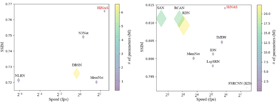
Figure 14: Trade-off between inference speed and performance. (a) denoising results of test on BSD200 when $\sigma=50$. (b) $\times$3 super-resolution results of test on BSD100. Marker size and color encode the number of parameters. HiNAS shows superior performance compared with a few recent methods.

Now we compare the HiNAS designed networks with a number of recent methods and use PSNR and SSIM to quantitatively measure the restoration performance of those methods. Table 10 shows the comparison results of denoising on BSD500 and Figure 12.

Table 10 shows that N3Net and HiNAS beat other models by a clear margin. Our proposed HiNAS achieves the best performance when $\sigma$ is set to 50 and 70. When the noise level $\sigma$ is set to 30, the SSIM of NLRN is slightly higher (0.002) than that of our HiNAS, but the PSNR of NLRN is much lower (nearly 1dB) than that of HiNAS.

Overall, our HiNAS achieves better performance than others. In addition, compared with the second best model N3Net, the network designed by HiNAS has fewer parameters and is faster in inference. As listed in Table 10, the HiNAS designed network has 0.34M parameters, which is 47.89% that of N3Net and 30.91% that of E-CAE. Compared with N3Net, the HiNAS designed network reduces the inference time on the test set of BSD500 by 79.92%.

The comparison results of $\times$ 4 super-resolution experiments are listed in Table 9 and more super-resolution experimental results of $\times$2, $\times$3 and $\times$4 are listed in Table 12. Compared with parameter heavy models which have more than 10 M parameters, HiNAS achieves lower PSNR and highly competitive SSIM, while having much faster inference speed and much fewer parameters. For instance, the network designed by HiNAS has only 0.33 M parameters, which is about $\nicefrac{{1}}{{47}}$ that of SAN. The inference speed is 20.97$\times$ that of SAN. Compared with fast super-resolution models, HiNAS achieves equal performance, while having faster inference speed. The recent method of FSRCNN (KD) leverages distillation to improve the performance of FSRCNN. This method has fewer parameters and faster inference speed compared with our HiNAS. However, the PSNR and SSIM of FSRCNN (KD) is much lower than ours and that of other fast super-resolution methods. So, we believe HiNAS is still comparable compared with FSRCNN (KD) when taking both inference speed and performance into consideration. Two examples are presented in Figure 13, from which we can draw two conclusions: 1) all three CNN based super-resolution models achieve significantly better visual results than bicubic; 2) slightly higher PSNR can not guarantee plausible visual results. In the first row, both SAN and IMDN achieve higher PSNR compared to HiNAS, but we can not see any difference from the results. In the second row, the PSNR and SSIM of the result of SAN are slightly higher than that of HiNAS, while the visual results of SAN and HiNAS are still very close, and it is hard to say which one is better. In summary, in terms of visual results, HiNAS is highly competitive with other state-of-the-art methods.

4.5 Trade-off between Inference Speed and Accuracy

We visualize in Figure 14 the performance comparison of our HiNAS and the state of the art in terms of the inference speed, SSIM and the number of parameters.

For image denoising, our HiNAS achieves advantages compared with other denoising networks. For image super-resolution, our HiNAS achieves the best trade-off between inference speed and performance. In terms of the inference speed, our HiNAS is only slower than FSRCNN (KD), but the performance of HiNAS are much better than that of FSRCNN (KD). Compared with other fast super-resolution networks, our HiNAS achieve higher SSIM, while having much faster inference speed and fewer parameters.

Table 12: Super-resolution experiments.

Method	Scale	Param. i (M)	time	Set5		Set14		BSD100		Urban100
			costs (s)	PSNR	SSIM	PSNR	SSIM	PSNR	SSIM	PSNR	SSIM
EDSR	$\times$2	43.00		38.11	0.9602	33.92	0.9195	32.32	0.9013	32.93	0.9351
SRMD	$\times$2	1.50		37.79	0.9601	33.32	0.9159	32.05	0.8985	31.33	0.9204
DBPN	$\times$2	10.05		38.09	0.9600	33.85	0.9190	32.27	0.9000	32.55	0.9324
RDN	$\times$2	22.30		38.24	0.9614	34.01	0.9212	32.34	0.9017	32.89	0.9353
RCAN	$\times$2	16.00		38.27	0.9614	34.11	0.9216	32.41	0.9026	33.34	0.9384
SAN	$\times$2	15.70		38.31	0.9620	34.07	0.9213	32.42	0.9028	33.10	0.9370
RFANet	$\times$2	11.00		38.26	0.9615	34.16	0.9220	32.41	0.9026	33.33	0.9026
bicubic	$\times$2	-	-	33.66	0.9299	30.24	0.8688	29.56	0.8431	26.88	0.8403
FSRCNN(KD)	$\times$2	0.013	0.67	37.33	0.9576	32.79	0.9105	31.65	0.8926	30.24	0.9071
VDSR	$\times$2	0.67		37.53	0.9590	33.05	0.9130	31.90	0.8960	30.77	0.9140
MemNet	$\times$2	0.68	8.50	37.78	0.9597	33.28	0.9142	32.08	0.8978	31.31	0.9195
FALSR-B	$\times$2	0.33	-	37.61	0.9582	33.29	0.9143	31.97	0.8967	31.28	0.9191
IDN	$\times$2	0.55	5.62	37.83	0.9600	33.30	0.9148	32.08	0.8985	31.27	0.9196
IMDN	$\times$2	0.69	2.47	38.00	0.9605	33.63	0.9177	32.19	0.8996	32.17	0.9283
HiNAS	$\times$2	0.23-0.28	2.04	37.65	0.9608	32.95	0.9191	31.97	0.9036	31.29	0.9236
SPSR	$\times$4	24.80	16.47	30.40	0.8627	26.64	0.7930	25.51	0.6576	29.41	0.8537
EDSR	$\times$4	43.00	-	32.46	0.8968	28.80	0.7876	27.71	0.7420	26.64	0.8033
SRMD	$\times$4	1.50	-	31.96	0.8925	28.35	0.7787	27.49	0.7337	25.68	0.7731
DBPN	$\times$4	10.00	-	32.47	0.8980	28.82	0.7860	27.72	0.7400	26.38	0.7946
RDN	$\times$4	22.30	10.71	32.47	0.8990	28.81	0.7871	27.72	0.7419	26.61	0.8028
RCAN	$\times$4	16.00	13.12	32.62	0.9001	28.86	0.7888	27.76	0.7435	26.82	0.8087
SAN	$\times$4	15.70	31.03	32.64	0.9003	28.92	0.7888	27.78	0.7436	26.79	0.8068
RFANet	$\times$4	11.00	-	32.66	0.9004	28.88	0.7894	27.79	0.7442	26.92	0.8112
bicubic	$\times$4	-	-	28.42	0.8104	26.00	0.7027	25.96	0.6675	23.14	0.6577
FSRCNN (KD)	$\times$4	0.013	0.54	30.95	0.8759	27.77	0.7615	27.08	0.7188	24.82	0.7393
VDSR	$\times$4	0.67	-	31.35	0.8830	28.02	0.7680	27.29	0.0726	25.18	0.7540
LapSRN	$\times$4	0.50	3.68	31.54	0.8852	28.09	0.7700	27.32	0.7275	25.21	0.7562
MemNet	$\times$4	0.68	6.86	31.74	0.8893	28.26	0.7723	27.40	0.7281	25.50	0.7630
IDN	$\times$4	0.55	2.47	31.82	0.8903	28.25	0.7730	27.41	0.7297	25.41	0.7632
IMDN	$\times$4	0.72	1.72	32.21	0.8948	28.58	0.7811	27.56	0.7353	26.04	0.7838
HiNAS	$\times$4	0.29-0.33	1.45	31.72	0.8926	27.85	0.7881	27.35	0.7465	25.51	0.7779

5 Conclusion

In this study, we have proposed HiNAS, an attempt of using NAS to automatically design effective network architectures for two low-level image restoration tasks, image denoising, and super-resolution. HiNAS builds a hierarchical search space including the inner search space and outer search space, which can search for the inner cell topological structures and outer layer widths, respectively.

We have proposed the layer-wise architecture sharing strategy to improve the flexibility of the search space, improving performance. We have also proposed a cell-sharing strategy to save memory, accelerating the search process. Finally, instead of searching for networks to learning the restoration result directly, our HiNAS design networks to learning the residual information between low-quality images and high-quality images. HiNAS is both memory and computation efficient, taking only less than $\nicefrac{{1}}{{6}}$ days to search using a single GPU. Extensive experimental results demonstrate that the proposed HiNAS achieves highly competitive performance compared with state-of-the-art models while having fewer parameters and faster inference speed. We believe that the proposed method can be applied to many other low-level image processing tasks.

References

- Ahn et al. (2018) Ahn N, Kang B, Sohn KA (2018) Fast, accurate, and lightweight super-resolution with cascading residual network. In: Proc. Eur. Conf. Comp. Vis., pp 252–268
- Bender et al. (2020) Bender G, Liu H, Chen B, Chu G, Cheng S, Kindermans PJ, Le QV (2020) Can weight sharing outperform random architecture search? an investigation with tunas. In: Proc. IEEE Conf. Comp. Vis. Patt. Recogn., pp 14323–14332
- Cai et al. (2018) Cai H, Chen T, Zhang W, Yu Y, Wang J (2018) Efficient architecture search by network transformation. In: Proc. AAAI Conf. Artificial Intell.
- Cai et al. (2019) Cai H, Wang T, Wu Z, Wang K, Lin J, Han S (2019) On-device image classification with proxyless neural architecture search and quantization-aware fine-tuning. In: Proc. Int. Conf. Computer Vision Workshops, pp 0–0
- Chatterjee and Milanfar (2009) Chatterjee P, Milanfar P (2009) Is denoising dead? IEEE Trans Image Process 19(4):895–911
- Chen et al. (2019) Chen S, Chen Y, Yan S, Feng J (2019) Efficient differentiable neural architecture search with meta kernels. arXiv preprint arXiv:191204749
- Chu et al. (2019a) Chu X, Zhang B, Ma H, Xu R, Li J, Li Q (2019a) Fast, accurate and lightweight super-resolution with neural architecture search. arXiv: Comp Res Repository abs/1901.07261
- Chu et al. (2019b) Chu X, Zhang B, Xu R, Ma H (2019b) Multi-objective reinforced evolution in mobile neural architecture search. arXiv: Comp Res Repository abs/1901.01074
- Dabov et al. (2007) Dabov K, Foi A, Katkovnik V, Egiazarian K (2007) Image denoising by sparse 3-d transform-domain collaborative filtering. IEEE Trans Image Process 16(8):2080–2095
- Dai et al. (2019) Dai T, Cai J, Zhang Y, Xia ST, Zhang L (2019) Second-order attention network for single image super-resolution. In: Proc. IEEE Conf. Comp. Vis. Patt. Recogn., pp 11065–11074
- Dong et al. (2015) Dong C, Loy CC, He K, Tang X (2015) Image super-resolution using deep convolutional networks. TPAMI 38(2):295–307
- Dong and Yang (2019a) Dong X, Yang Y (2019a) Network pruning via transformable architecture search. arXiv preprint arXiv:190509717
- Dong and Yang (2019b) Dong X, Yang Y (2019b) One-shot neural architecture search via self-evaluated template network. In: Proc. IEEE Conf. Comp. Vis. Patt. Recogn., pp 3681–3690
- Dong and Yang (2019c) Dong X, Yang Y (2019c) Searching for a robust neural architecture in four gpu hours. In: Proc. IEEE Conf. Comp. Vis. Patt. Recogn., pp 1761–1770
- Elsken et al. (2018) Elsken T, Metzen JH, Hutter F (2018) Efficient multi-objective neural architecture search via lamarckian evolution. arXiv: Comp Res Repository abs/1804.09081
- Fang et al. (2020) Fang J, Sun Y, Zhang Q, Li Y, Liu W, Wang X (2020) Densely connected search space for more flexible neural architecture search. In: Proc. IEEE Conf. Comp. Vis. Patt. Recogn.
- Ghiasi et al. (2019) Ghiasi G, Lin TY, Le Q (2019) NAS-FPN: Learning scalable feature pyramid architecture for object detection. In: Proc. IEEE Conf. Comp. Vis. Patt. Recogn., pp 7036–7045
- Gu et al. (2014) Gu S, Zhang L, Zuo W, Feng X (2014) Weighted nuclear norm minimization with application to image denoising. In: Proc. IEEE Conf. Comp. Vis. Patt. Recogn., pp 2862–2869
- Guo et al. (2019) Guo S, Yan Z, Zhang K, Zuo W, Zhang L (2019) Toward convolutional blind denoising of real photographs. In: Proc. IEEE Conf. Comp. Vis. Patt. Recogn., pp 1712–1722
- Guo et al. (2020) Guo Z, Zhang X, Mu H, Heng W, Liu Z, Wei Y, Sun J (2020) Single path one-shot neural architecture search with uniform sampling. In: European Conference on Computer Vision, Springer, pp 544–560
- He et al. (2016) He K, Zhang X, Ren S, Sun J (2016) Identity mappings in deep residual networks. In: Proc. Eur. Conf. Comp. Vis., Springer, pp 630–645
- He et al. (2018) He Y, Lin J, Liu Z, Wang H, Li LJ, Han S (2018) Amc: Automl for model compression and acceleration on mobile devices. In: Proc. Eur. Conf. Comp. Vis., pp 784–800
- Hu et al. (2018) Hu J, Shen L, Sun G (2018) Squeeze-and-excitation networks. In: Proc. IEEE Conf. Comp. Vis. Patt. Recogn., pp 7132–7141
- Hui et al. (2018) Hui Z, Wang X, Gao X (2018) Fast and accurate single image super-resolution via information distillation network. In: Proc. IEEE Conf. Comp. Vis. Patt. Recogn., pp 723–731
- Hui et al. (2019) Hui Z, Gao X, Yang Y, Wang X (2019) Lightweight image super-resolution with information multi-distillation network. In: Proc. ACM Int. Conf. Multimedia, pp 2024–2032
- Jaroensri et al. (2019) Jaroensri R, Biscarrat C, Aittala M, Durand F (2019) Generating training data for denoising real rgb images via camera pipeline simulation. arXiv: Comp Res Repository abs/1904.08825
- Kim et al. (2016a) Kim J, Kwon Lee J, Mu Lee K (2016a) Accurate image super-resolution using very deep convolutional networks. In: Proc. IEEE Conf. Comp. Vis. Patt. Recogn., pp 1646–1654
- Kim et al. (2016b) Kim J, Kwon Lee J, Mu Lee K (2016b) Deeply-recursive convolutional network for image super-resolution. In: Proc. IEEE Conf. Comp. Vis. Patt. Recogn., pp 1637–1645
- Lai et al. (2017) Lai WS, Huang JB, Ahuja N, Yang MH (2017) Deep laplacian pyramid networks for fast and accurate super-resolution. In: Proc. IEEE Conf. Comp. Vis. Patt. Recogn., pp 624–632
- Lee et al. (2020) Lee W, Lee J, Kim D, Ham B (2020) Learning with privileged information for efficient image super-resolution. arXiv: Comp Res Repository abs/2007.07524
- Li and Talwalkar (2020) Li L, Talwalkar A (2020) Random search and reproducibility for neural architecture search. In: Proc. Uncertainty in Artificial Intelligence, pp 367–377
- Liang et al. (2019) Liang H, Zhang S, Sun J, He X, Huang W, Zhuang K, Li Z (2019) Darts+: Improved differentiable architecture search with early stopping. arXiv: Comp Res Repository abs/1909.06035
- Lim et al. (2017) Lim B, Son S, Kim H, Nah S, Mu Lee K (2017) Enhanced deep residual networks for single image super-resolution. In: Proc. IEEE Conf. Computer vision and Pattern Recognition Workshops, pp 136–144
- Liu et al. (2019a) Liu C, Chen LC, Schroff F, Adam H, Hua W, Yuille AL, Fei-Fei L (2019a) Auto-Deeplab: Hierarchical neural architecture search for semantic image segmentation. In: Proc. IEEE Conf. Comp. Vis. Patt. Recogn., pp 82–92
- Liu et al. (2018a) Liu D, Wen B, Fan Y, Loy CC, Huang TS (2018a) Non-local recurrent network for image restoration. In: Proc. Advances in Neural Inf. Process. Syst., pp 1673–1682
- Liu et al. (2018b) Liu H, Simonyan K, Vinyals O, Fernando C, Kavukcuoglu K (2018b) Hierarchical representations for efficient architecture search. In: Proc. Int. Conf. Learn. Representations
- Liu et al. (2019b) Liu H, Simonyan K, Yang Y (2019b) Darts: Differentiable architecture search. In: Proc. Int. Conf. Learn. Representations
- Liu et al. (2020) Liu J, Zhang W, Tang Y, Tang J, Wu G (2020) Residual feature aggregation network for image super-resolution. In: Proc. IEEE Conf. Comp. Vis. Patt. Recogn., pp 2359–2368
- Liu et al. (2019c) Liu P, El Basha M, Li Y, Xiao Y, Sanelli P, Fang R (2019c) Deep evolutionary networks with expedited genetic algorithms for medical image denoising. Medical Image Analysis 54:306–315
- Liu et al. (2019d) Liu X, Suganuma M, Sun Z, Okatani T (2019d) Dual residual networks leveraging the potential of paired operations for image restoration. In: Proc. IEEE Conf. Comp. Vis. Patt. Recogn., pp 7007–7016
- Loshchilov and Hutter (2017) Loshchilov I, Hutter F (2017) Sgdr: Stochastic gradient descent with warm restarts. In: Proc. Int. Conf. Learn. Representations
- Ma et al. (2018) Ma N, Zhang X, Zheng HT, Sun J (2018) Shufflenet v2: Practical guidelines for efficient cnn architecture design. In: Proc. Eur. Conf. Comp. Vis., pp 116–131
- Mao et al. (2016) Mao X, Shen C, Yang YB (2016) Image restoration using very deep convolutional encoder-decoder networks with symmetric skip connections. In: Proc. Advances in Neural Inf. Process. Syst., pp 2802–2810
- Martin et al. (2001) Martin D, Fowlkes C, Tal D, Malik J, et al. (2001) A database of human segmented natural images and its application to evaluating segmentation algorithms and measuring ecological statistics. In: Proc. IEEE Int. Conf. Comp. Vis., pp 416–423
- Nekrasov et al. (2019) Nekrasov V, Chen H, Shen C, Reid I (2019) Fast neural architecture search of compact semantic segmentation models via auxiliary cells. In: Proc. IEEE Conf. Comp. Vis. Patt. Recogn., pp 9126–9135
- Pham et al. (2018) Pham H, Guan MY, Zoph B, Le QV, Dean J (2018) Efficient neural architecture search via parameter sharing. In: Proc. Int. Conf. Mach. Learn.
- Plötz and Roth (2018) Plötz T, Roth S (2018) Neural nearest neighbors networks. In: Proc. Advances in Neural Inf. Process. Syst., pp 1087–1098
- Suganuma et al. (2018) Suganuma M, Ozay M, Okatani T (2018) Exploiting the potential of standard convolutional autoencoders for image restoration by evolutionary search. In: Proc. Int. Conf. Mach. Learn.
- Szegedy et al. (2015) Szegedy C, Wei L, Jia Y, Sermanet P, Rabinovich A (2015) Going deeper with convolutions. In: Proc. IEEE Conf. Comp. Vis. Patt. Recogn.
- Szegedy et al. (2016) Szegedy C, Vanhoucke V, Ioffe S, Shlens J, Wojna Z (2016) Rethinking the inception architecture for computer vision. In: Proc. IEEE Conf. Comp. Vis. Patt. Recogn., pp 2818–2826
- Szegedy et al. (2017) Szegedy C, Ioffe S, Vanhoucke V, Alemi A (2017) Inception-v4, inception-resnet and the impact of residual connections on learning. In: Proc. AAAI Conf. Artificial Intell.
- Tai et al. (2017) Tai Y, Yang J, Liu X, Xu C (2017) Memnet: A persistent memory network for image restoration. In: Proc. IEEE Int. Conf. Comp. Vis., pp 4539–4547
- Tan et al. (2019) Tan M, Chen B, Pang R, Vasudevan V, Sandler M, Howard A, Le Q (2019) Mnasnet: Platform-aware neural architecture search for mobile. In: Proc. IEEE Conf. Comp. Vis. Patt. Recogn., pp 2820–2828
- Tobias Plötz (2018) Tobias Plötz SR (2018) Neural nearest neighbors networks. In: Proc. Advances in Neural Inf. Process. Syst., pp 1673–1682
- Wan et al. (2020) Wan A, Dai X, Zhang P, He Z, Tian Y, Xie S, Wu B, Yu M, Xu T, Chen K, Vajda P, Gonzalez JE (2020) Fbnetv2: Differentiable neural architecture search for spatial and channel dimensions. In: Proc. IEEE Conf. Comp. Vis. Patt. Recogn., pp 12965–12974
- Wang et al. (2020) Wang N, Gao Y, Chen H, Wang P, Tian Z, Shen C (2020) NAS-FCOS: Fast neural architecture search for object detection. In: Proc. IEEE Conf. Comp. Vis. Patt. Recogn.
- Wang et al. (2004) Wang Z, Bovik A, Sheikh H, Simoncelli E (2004) Image quality assessment: from error visibility to structural similarity. IEEE Trans Image Process 13(4):600–612
- Wu et al. (2019) Wu B, Dai X, Zhang P, Wang Y, Sun F, Wu Y, Tian Y, Vajda P, Jia Y, Keutzer K (2019) Fbnet: Hardware-aware efficient convnet design via differentiable neural architecture search. In: Proc. IEEE Conf. Comp. Vis. Patt. Recogn., pp 10734–10742
- Wu et al. (2020) Wu X, Liu M, Cao Y, Ren D, Zuo W (2020) Unpaired learning of deep image denoising. In: European Conference on Computer Vision, Springer, pp 352–368
- Xu et al. (2021) Xu Y, Xie L, Dai W, Zhang X, Chen X, Qi GJ, Xiong H, Tian Q (2021) Partially-connected neural architecture search for reduced computational redundancy. IEEE Trans Pattern Anal Mach Intell
- Zhang et al. (2018a) Zhang C, Ren M, Urtasun R (2018a) Graph hypernetworks for neural architecture search. arXiv: Comp Res Repository abs/1810.05749
- Zhang et al. (2020) Zhang H, Li Y, Chen H, Shen C (2020) Memory-efficient hierarchical neural architecture search for image denoising. In: Proc. IEEE Conf. Comp. Vis. Patt. Recogn., pp 3657–3666
- Zhang et al. (2017a) Zhang K, Zuo W, Chen Y, Meng D, Zhang L (2017a) Beyond a gaussian denoiser: Residual learning of deep cnn for image denoising. IEEE Trans Image Process 26(7):3142–3155
- Zhang et al. (2017b) Zhang K, Zuo W, Gu S, Zhang L (2017b) Learning deep CNN denoiser prior for image restoration. In: Proc. IEEE Conf. Comp. Vis. Patt. Recogn., pp 3929–3938
- Zhang et al. (2018b) Zhang K, Zuo W, Zhang L (2018b) FFDNet: Toward a fast and flexible solution for CNN-based image denoising. IEEE Trans Image Process 27(9):4608–4622
- Zhang et al. (2018c) Zhang K, Zuo W, Zhang L (2018c) Learning a single convolutional super-resolution network for multiple degradations. In: Proc. IEEE Conf. Comp. Vis. Patt. Recogn., pp 3262–3271
- Zhang et al. (2018d) Zhang Y, Li K, Li K, Wang L, Zhong B, Fu Y (2018d) Image super-resolution using very deep residual channel attention networks. In: Proc. Eur. Conf. Comp. Vis., pp 286–301
- Zhang et al. (2018e) Zhang Y, Tian Y, Kong Y, Zhong B, Fu Y (2018e) Residual dense network for image super-resolution. In: Proc. IEEE Conf. Comp. Vis. Patt. Recogn., pp 2472–2481
- Zhong et al. (2018) Zhong Z, Yan J, Wu W, Shao J, Liu CL (2018) Practical block-wise neural network architecture generation. In: Proc. IEEE Conf. Comp. Vis. Patt. Recogn., pp 2423–2432
- Zoph and Le (2017) Zoph B, Le QV (2017) Neural architecture search with reinforcement learning. In: Proc. Int. Conf. Learn. Representations
- Zoph et al. (2018) Zoph B, Vasudevan V, Shlens J, Le QV (2018) Learning transferable architectures for scalable image recognition. In: Proc. IEEE Conf. Comp. Vis. Patt. Recogn., pp 8697–8710