Robust Exponential Mixing and Convergence to Equilibrium for Singular-Hyperbolic Attracting Sets

Abstract.

We extend results on robust exponential mixing for geometric Lorenz attractors, with a dense orbit and a unique singularity, to singular-hyperbolic attracting sets with any number of (either Lorenz- or non-Lorenz-like) singularities and finitely many ergodic physical/SRB invariant probability measures, whose basins cover a full Lebesgue measure subset of the trapping region of the attracting set.

We obtain exponential mixing for any physical probability measure supported in the trapping region and also exponential convergence to equilibrium, for a $C^{2}$ open subset of vector fields in any $d$-dimensional compact manifold ($d\geq 3$).

1. Introduction

The expression “statistical properties” of a Dynamical System refers to the statistical behavior of typical trajectories of the system. It is well-known that this behavior is related to properties of the evolution of measures under the dynamics. Statistical properties are frequently a simpler object to study than pointwise behaviour of trajectories, which is most of the time unpredictable. However, statistical properties are regular for most known systems and mostly admit a simple description.

The statistical tools provided by Differentiable Ergodic Theory are among the most powerful techniques available to study the global asymptotic behavior of Dynamical Sytems. A central concept is that of physical measure (or Sinai-Ruelle-Bowen measure) for a flow or a transformation. Such measure for a flow $X_{t}$ on a compact manifold is an invariant probability measure $\mu$ for which the family of points $z$ satisfying

$$\lim_{t\to+\infty}\frac{1}{t}\int_{0}^{t}\psi\big{(}X_{s}(z)\big{)}\,ds=\int\psi\,d\mu,$$

for all continuous observables (functions) $\psi$. That is, the time averages of a continuous observable along the trajectory of $z$ converge to the space average of the same observable with respect to $\mu$; and the set of all these points is a positive Lebesgue (volume) measure subset $B(\mu)$ (the ergodic basin) of the ambient space.

These time averages are considered a priori physically observable when dealing with a mathematical model of some real phenomenon whose properties can be measurable.

This kind of measures was first rigorously obtained for (uniformly) hyperbolic diffeomorphisms by Sinai, Ruelle and Bowen [48, 47, 24]. For non uniformly hyperbolic transformations and flows these measures were studied more recently: we mention only the results closer to the present text in [17, 35, 18], on the existence of physical measures for singular-hyperbolic attractors. Statistical properties of such measures are an active field of study: among the article used in this work we stress [4, 32, 19, 8, 12, 13].

The general motivation is that the family $\{\psi\circ X_{t}\}_{t\geq 0}$ should behave asymptotically as a family of independent and identically distributed random variables.

An important property is the speed of convergence of the time average to the space average among many others. Considering $\varphi$ and $\psi\circ X_{t}:M\to{\mathbb{R}}$ as random variables with law $\mu$, mixing means that the random variables $\varphi$ and $\psi\circ X_{t}$ are asymptotically independent: ${\mathbb{E}}\big{(}\varphi\cdot(\psi\circ X_{t})\big{)}$ converges to ${\mathbb{E}}(\varphi)\cdot{\mathbb{E}}(\psi)$ when $t$ grown without bound. Writting the correlation function

$$C_{t}(\varphi,\psi) ={\mathbb{E}}\big{(}\psi\cdot(\varphi\circ X_{t})\big{)}-{\mathbb{E}}(\varphi)\cdot{\mathbb{E}}(\psi)=\int\psi\cdot\big{(}\varphi\circ X_{t}\big{)}\,d\mu-\int\varphi\,d\mu\int\psi\,d\mu$$

we get $|C_{t}(\varphi,\psi)|\xrightarrow[t\to\infty]{}0$ for all integrable observables in case of mixing. Exponential mixing means that there exist $C,\gamma>0$ so that

$$|C_{t}(\psi,\varphi)|\leq Ce^{-\gamma t}\|\psi\|\|\varphi\|,\quad t>0;$$

while superpolynomial mixing holds if for all $\beta>0$ we can find $C_{\beta}>0$ for which

$$|C_{t}(\psi,\varphi)|\leq C_{\beta}t^{-\beta}\|\psi\|\|\varphi\|,\quad t>0;$$

on a Banach space of usually more regular observables than just integrable ones (mostly Hölder continuous, some times differentiable).

To ascertain the speed of mixing is a subtle issue for flows. In spite of exponential mixing having been prived for hyperbolic diffeomorphisms for Sinai, Ruelle and Bowen [48, 47, 24] in the 70’s, only in the final years of the XXth century a significant breakthrough was obtained in the fundamental work of Dolgopyat [29]. Here the author obtained for the first time exponential mixing for Anosov flows with respect to physical measures under rather strong assumptions (global smoothness of stable and unstable foliations and their uniform non-integrability). These assumptions are not robust, i.e., the family of systems which satisfy these assumptions loose these properties by small perturbations.

Later superpolynomial mixing was obtained for open and dense families (hence robust) of hyperobolic flows by Field, Melbourne and Torok [31] refining Dolgopyat techniques, but only achieving a slower mixing speed.

Singular-hyperbolicity is a non-trivial recent extension of the notion of uniform hyperbolicity that encompassses systems like the Lorenz attractor in a unified theory, founded on the work of Morales, Pacifico and Pujals [41]. This allows to rigorously frame Lorenz-like attractors after the the work of Tucker [50].

For singular-hyperbolic attracting sets the existence of physical measures and some of their properties were obtained for the first time in [17]. Surprinsingly it was easier to obtain robust exponential mixing for physical measures among Lorenz-like attractors – this was first proved by Araujo and Varandas in [19] for an open subset of vector fields with a geometric Lorenz attractor – than among hyperoblic attractors or even Anosov flows.

For the original Lorenz attractor exponentially mixing was proved by the works of Araujo, Melbourne and Varandas [13, 10] and recently Araujo and Melbourne [12] proved superpolynomial mixing for an open an dense subset of singular-hyperbolic attracting sets.

The same techniques allow us to obtain robust exponential mixing for Axiom A attractors [8] and have been recently extended to achieve robust exponential mixing for Anosov flows [26]. Still more recently [49] explores the same technique to get exponential mixing for all equilibrium states (of which physical measure are but an example) with respect to Hölder continuous potentials for an open and dense subset of topologically mixing $C^{\infty}$ Anosov flows on $3$-manifolds.

An interesting variation of the theme is the convergence to equilibrium: replacing $\mu$ by the Lebesgue (volume) measure we consider the following function

$$E_{t}(\psi,\varphi)=\int(\varphi\circ X_{t})\,\psi\;d\operatorname{Leb}-\int\psi\;d\operatorname{Leb}\int\varphi\;d\mu$$

and if we have convergence $|E_{t}(\psi,\varphi)|\to 0$ this means, in particular (letting $\psi\equiv 1$), that for a certain (usually fairly regular) class of observables

$$\lim_{t\to\infty}\int\varphi\circ X_{t}\,d\operatorname{Leb}=\int\varphi\,d\mu$$

which, a priori, allows us to use a “natural” measure to estimate $\mu$ through experimental observations of the system.

In this work we extend the result of robust exponential mixing for the $3$-dimensional geometric Lorenz attractor, with a unique singularity and a dense orbit, to singular-hyperbolic attracting set, with any number of singularities (Lorenz-like or not), finite number of invariant ergodic physical probability measures and higher dimensional stable bundle. We obtain exponential mixing for all physical measures supported on the trapping region of the attracting set and also exponential convergence to equilibrium, for a $C^{2}$-open subset of vector fields on compact $d$-manifold ($d\geq 3$).

1.1. Preliminary definitions

Let $M$ be a compact boundaryless $d$-dimensional manifold. Given an integer $k\geq 1$, we denote by ${\mathfrak{X}}^{k}(M)$ the set of $C^{k}$ vector fields on $M$ endowed with the $C^{k}$ topology. We fix some smooth Riemannian structure on $M$ and we denote the distance induced by this structure by $\operatorname{dist}$ and the volume measure by $\operatorname{Leb}$. We may assume that both $\operatorname{dist}$ and $\operatorname{Leb}$ are normalized, that is, the diameter of $M$, denoted here by $\operatorname{diam}(M)$, and $\operatorname{Leb}(M)$ are equal to $1$.

Given $X\in{{\mathfrak{X}}}^{k}(M)$ we denote by $X_{t}:M\to M$, $t\in{\mathbb{R}}$, the flow induced by $X$. For each $x\in M$ and each interval $I\subset{\mathbb{R}}$ we set $X_{I}(x):=\{X_{t}(x):\ t\in I\}$. In general, given a point $x\in M$ we denote the orbit of $x$ by the flow of $X$ by the set $\mathcal{O}_{X}(x)=X_{{\mathbb{R}}}(x)$.

We say that $x\in M$ is regular for the vector field $X$ if $X(x)\neq 0$. Otherwise we say that $x$ is an equilibrium or singularity of $X$. We also say that the corresponding orbit is regular or singular, respectively. If $\sigma\in M$ is a singularity for $X$ then $\sigma$ is a fixed point for the flow of $X$, that is, $X_{t}(\sigma)=\sigma$ for all $t\in{\mathbb{R}}$. We say that $p\in M$ is a periodic point (or the orbit of $p$ is periodic) for $X$, if the set $\{t\in{\mathbb{R}}^{+}:\ X_{t}(p)=p\}$ is nonempty and the number $T:=\inf\{t\in{\mathbb{R}}^{+}:\ X_{t}(p)=p\}$ is positive. In this case we call $T$ the period of $p$.

We say that a set $\Lambda\subset M$ is invariant by $X$ if $X_{t}(\Lambda)=\Lambda$ for all $t\in{\mathbb{R}}$. A compact invariant set $\Lambda$ for $X$ is said to be isolated if we can find an open neighborhood $U\supset\Lambda$ so that $\Lambda=\bigcap_{t\in{\mathbb{R}}}X_{t}(U)$. If $U$ also satisfies $\overline{X_{t}(U)}\subset U$ for all $t>0$ then we say that $\Lambda$ is an attracting set and that $U$ is a trapping region for $\Lambda$. In this case we have that $\Lambda=\cap_{t>0}X_{t}(U)$. The topological basin of an attracting set $\Lambda$ is given by

$$W^{s}(\Lambda)=\left\{x\in M:\lim_{t\to+\infty}\operatorname{dist}\big{(}X_{t}(x),\Lambda\big{)}=0\right\}.$$

Given $x\in M$ the $\omega$-limit set of $x$ by the flow $X_{t}$ is given by the set

$$\omega(x)=\omega_{X}(x)=\left\{y\in M:\ \exists t_{k}\nearrow+\infty\text{ such that }\lim_{k\to+\infty}\operatorname{dist}(X_{t_{k}}(x),y)=0\right\}.$$

An invariant set $\Lambda$ is transitive for $X$ if there exists a regular point $x\in M$ such that $\Lambda=\omega_{X}(x)$. We say that $\Lambda$ is non-trivial if it is neither a finite set of periodic orbits nor a finite set of equilibria. Otherwise we say that $\Lambda$ is trivial.

A compact invariant set $\Lambda\subset M$ is an attractor for a vector field $X$ if it is a transitive attracting set for $X$. We say that the attractor is proper if it is not the whole ambient manifold $M$.

1.1.1. Singular-hyperbolic attracting sets

Let $\Lambda$ be a compact invariant set for $X\in{\mathfrak{X}}^{r}(M)$ for some $r\geq 1$. We say that $\Lambda$ is partially hyperbolic if the tangent bundle over $\Lambda$ can be written as a continuous $DX_{t}$-invariant sum

$$T_{\Lambda}M=E^{s}\oplus E^{cu},$$

where $d_{s}=\dim E^{s}_{x}\geq 1$ and $d_{cu}=\dim E^{cu}_{x}\geq 2$ for $x\in\Lambda$, and there exist constants $C>0$, $\lambda\in(0,1)$ such that for all $x\in\Lambda$, $t\geq 0$, we have

• uniform contraction along $E^{s}$: $\|DX_{t}|E^{s}_{x}\|\leq C\lambda^{t};$

• domination of the splitting: $\|DX_{t}|E^{s}_{x}\|\cdot\|DX_{-t}|E^{cu}_{X_{t}x}\|\leq C\lambda^{t}.$

We refer to $E^{s}$ as the stable bundle and to $E^{cu}$ as the center-unstable bundle. A partially hyperbolic attracting set is a partially hyperbolic set that is also an attracting set.

The center-unstable bundle $E^{cu}$ is volume expanding if there exists $K,\theta>0$ such that $|\det(DX_{t}|E^{cu}_{x})|\geq Ke^{\theta t}$ for all $x\in\Lambda$, $t\geq 0$.

Definition 1.1.

Let $\Lambda$ be a compact invariant set for $X\in{{\mathfrak{X}}}^{r}(M)$. We say that $\Lambda$ is a singular-hyperbolic set if all equilibria in $\Lambda$ are hyperbolic, and $\Lambda$ is partially hyperbolic with volume expanding two-dimensional center-unstable bundle ($d_{cu}=2$). A singular-hyperbolic set which is also an attracting set is called a singular-hyperbolic attracting set.

Remark 1.2.

A singular-hyperbolic attracting set contains no isolated periodic orbits. For such a periodic orbit would have to be a periodic sink, violating volume expansion.

Theorem 1.3.

[40, Lemma 3] Every compact invariant set without singularities of a singular-hyperbolic set is hyperbolic.

A subset $\Lambda\subset M$ is transitive if it has a full dense orbit, that is, there exists $x\in\Lambda$ such that $\overline{\{X_{t}x:t\geq 0\}}=\Lambda=\overline{\{X_{t}x:t\leq 0\}}$.

Definition 1.4.

A singular-hyperbolic attractor is a transitive singular-hyperbolic attracting set.

Proposition 1.5.

[12, Proposition 2.6] Suppose that $\Lambda$ is a singular-hyperbolic attractor and let $\sigma\in\Lambda$ be an equilibrium. Then $\sigma$ is Lorenz-like. That is, $DG(\sigma)|E^{cu}_{\sigma}$ has real eigenvalues $\lambda^{s}$, $\lambda^{u}$ satisfying $-\lambda^{u}<\lambda^{s}<0<\lambda^{u}$.

Remark 1.6.

Some consequences of singular-hyperbolicity follow.

1. Partial hyperbolicity of $\Lambda$ implies that the direction $X(x)$ of the flow is contained in the center-unstable bundle $E^{cu}_{x}$ at every point $x$ of $\Lambda$ (see [7, Lemma 5.1]).

2. The index of a singularity $\sigma$ in a singular-hyperbolic set $\Lambda$ equals either $\dim E^{s}$ or $1+\dim E^{s}$. That is, $\sigma$ is either a hyperbolic saddle with $\dim M-\dim E^{s}_{\sigma}=2$ (that is, the codimension of $E^{s}_{\sigma}$ equals $2$) or a Lorenz-like singularity.

3. If a singularity $\sigma$ in a singular-hyperbolic set $\Lambda$ is not Lorenz-like, then there is no regular orbit of $\Lambda$ that accumulates $\sigma$ in the positive time direction. In other words, there is no $x\in\Lambda$ regular such that $\sigma\in\omega(x)$ (see [18, Remark 1.5])

Definition 1.7.

A singular-hyperbolic invariant set is nontrivial if it is a non-trivial compact invariant subset which contains some Lorenz-like equilibrium.

1.1.2. Physical measures

The existence of a unique invariant and ergodic physical measure for singular-hyperbolic attractors was first proved for $3$-dimensional manifolds in [17] and extended to singular-hyperbolic attracting sets in e.g. [18]. For sectional-hyperbolic attractors, existence and uniqueness of physical measure was obtained in [35] and recently extended to attracting sets in [6]. In fact, sectional-hyperbolic attracting sets have finitely many ergodic physical measures which are equilibrium states for the central-unstable Jacobian, just like Axiom A attracting sets.

Theorem 1.8.

[18, Theorem 1.7] Let $\Lambda$ be a singular-hyperbolic attracting set for a $C^{2}$ vector field $X$ with the open subset $U$ as trapping region. Then

1. there are finitely many ergodic physical/SRB measures $\mu_{1},\dots,\mu_{k}$ supported in $\Lambda$ such that the union of their ergodic basins covers $U$ Lebesgue almost everywhere: $\operatorname{Leb}\left(U\setminus\big{(}\bigcup_{i=1}^{k}B(\mu_{i})\big{)}\right)=0.$

2. Moreover, for each $X$-invariant ergodic probability measure $\mu$ supported in $\Lambda$ the following are equivalent

   1. $h_{\mu}(X_{1})=\int\log|\det DX_{1}\mid_{E^{cu}}|\,d\mu>0$;

   2. $\mu$ is a $SRB$ measure, that is, admits an absolutely continuous disintegration along unstable manifolds;

   3. $\mu$ is a physical measure, i.e., its basin $B(\mu)$ has positive Lebesgue measure.

3. The family ${\mathbb{E}}$ of all $X$-invariant probability measures which satisfy item (2a) above is the convex hull ${\mathbb{E}}=\left\{\sum_{i=1}^{k}t_{i}\mu_{i}:\sum_{i}t_{i}=1;0\leq t_{i}\leq 1,i=1,\dots,k\right\}.$

We note that there are many examples of singular-hyperbolic attracting sets, non-transitive and containing non-Lorenz-like singularities; see Subsection 2.2.

1.2. Statement of results

We can now state our main results. In what follows, we write $C^{k+\eta}(M)$, where $\eta\in(0,1]$ is a real number and $k\geq 0$ is a non-negative integer, for the set of functions $\varphi:M\to{\mathbb{R}}$ which are of class $C^{k}$ and the $k$th derivative $D^{k}\varphi$ is $\eta$-Hölder. This is a Banach space with norm given by

$$\|\varphi\|_{k+\eta}:=\sum_{i=0}^{k}|D^{i}\varphi|_{\infty}+|D^{k}\varphi|_{\eta},$$

where for any function $\psi:M\to{\mathbb{R}}$ we set $|\psi|_{\infty}:=\sup_{x\in M}|\psi(x)|$ and $|\psi|_{\eta}:=\sup_{x\neq y}|\psi(x)-\psi(y)|/\operatorname{dist}(x,y)^{\eta}$.

Theorem A (Exponential mixing).

There exists an open subset $\mathcal{U}\subset{\mathfrak{X}}^{2}(M)$ such that each vector field $X\in\mathcal{U}$ admits a non-trivial connected singular-hyperbolic attracting set $\Lambda$ such that, given $X\in\mathcal{U}$ and $\mu$ a physical measure supported in $\Lambda$, there exist constants $c,C>0$ such that for any $\eta\in(0,1]$ we have $|C_{t}(\varphi,\psi)|\leq Ce^{-ct}\|\varphi\|_{\eta}\|\psi\|_{\eta},$ for all $\varphi,\psi\in C^{\eta}(M)$ and $t>0$.

We can also present this result with a different appearence. If $\mu_{1},\dots,\mu_{k}$ are the ergodic invariant physical probability measures of $X$ supported in $\Lambda$ as given by Theorem 1.8 and $\vartheta_{i}=\operatorname{Leb}(B(\mu_{i}))$ is the volume of each of their basins, then the normalized Lebesgue measure, on a trapping region $U$ for $\Lambda$, can be written as a linear convex combination $\operatorname{Leb}=\sum_{i}\vartheta_{i}\operatorname{Leb}_{i}$ where $\operatorname{Leb}_{i}=\vartheta_{i}^{-1}\operatorname{Leb}\mid_{B(\mu_{i})}$.

Corollary B (Exponential convergence to equilibrium).

In the same setting of Theorem A, for each $0<\eta\leq 1$ there exist constants $c,C>0$ such that

$$\left|\int(\varphi\circ X_{t})\psi\,d\operatorname{Leb}-\int\varphi\,d\widetilde{\mu}\int\psi\,d\operatorname{Leb}\right|\leq Ce^{-ct}\|\varphi\|_{\eta}\|\psi\|_{\eta},$$

for all $\varphi,\psi\in C^{\eta}(M)$ and $t>0$, where $\widetilde{\mu}=\sum_{i}\vartheta_{i}\mu_{i}$.

If we are dealing with an attractor, that is, if $\Lambda$ is transitive, then there is a unique physical measure and putting $\psi\equiv 1$ in the statement of Corollary B we get $\big{|}\int\varphi\circ X_{t}\,d\operatorname{Leb}-\int\varphi\,d\mu\big{|}\leq Ce^{-ct}|\varphi|_{C^{1}}$ for all $\varphi\in C^{1}(M)$ and all $t>0$, that is, $(X_{t})_{*}\operatorname{Leb}$ converges exponentially fast to the physical (also known as “natural”) measure $\mu$ in the weak-* topology when $t$ goes to infinity.

1.3. Some consequences of fast mixing

It is known that fast decay of correlations for a dynamical system implies many other statistical properties.

The base map of a hyperbolic skew-product semiflow is known to satisfy exponential mixing for Hölder observables with respect to its physical measures; see e.g. [9]. This in turn automatically implies certain statistical properties for the induced measure on the suspension flow: the Central Limit Theorem, the Law of the Iterated Logarithm and the Almost Sure Invariance Principle; see e.g. [37].

For mixing and the speed of mixing, the properties of the base map do not extend to the suspension flow in general: the suspension flow does not even have to be mixing. More precisely, see [46], rates of mixing of suspension flows can be arbitrarily slow even if the base map is exponentially mixing.

Having a flow which mixes exponentially fast should imply more subtle statistical properties. In fact, some statistical properties of the time-$1$ map of singular-hyperbolic flows near attracting sets can be obtained in this way.

Corollary C (Consequences of exponential mixing for the time-$1$ map).

Let $\mathcal{U}$ be as in Theorem 2.5. Given $X\in\mathcal{U}$, let $\mu$ be an ergodic physical measure for the singular-hyperbolic attracting set $\Lambda$. For all $\varphi\in C^{1}(M)$ it holds:

1. (Central Limit Theorem (CLT) for the time-$1$ map). There exists $\sigma\geq 0$ such that we have the following convergence in distribution

   $$\dfrac{1}{\sqrt{n}}\left[\sum^{n-1}_{j=0}\varphi\circ X_{j}-n\int\varphi\,d\mu\right]\xrightarrow[n\to+\infty]{{\mathcal{D}}}{\mathcal{N}}(0,\sigma^{2})$$

   Moreover, if $\sigma=0$, then for every periodic point $q\in\Lambda$, there exists $T>0$ (independent of $\varphi$) such that $\int^{T}_{0}\varphi(X_{t}(q))\,dt=0$.

2. (Almost Sure Invariant Principle (ASIP) for the time-$1$ map). Passing to an enriched probability space, there exists a sequence $Y_{0},Y_{1},\dots$ of iid normal random variables with mean zero and variance $\sigma^{2}$ such that

   $$\sum^{n-1}_{j=0}\varphi\circ X_{j}=n\int\varphi\,d\mu+\sum^{n-1}_{j=0}Y_{j}+\mathcal{O}(\sqrt[4]{n\log\log n}\sqrt{\log n}),\ a.e.$$

This corollary follows from the proof of exponential mixing just as in [13], where the same was deduced from superpolynomial decay of correlations.

The ASIP implies the CLT and also the functional CLT (weak invariance principle), and the law of the iterated logarithm together with its functional version, as well as numerous other results. The reader should consult [45] for a comprehensive list.

1.3.1. Organization of the text

The remainder of the paper is organized as follows.

In Section 2 we present the overall organization of the proof, open classes of examples in the setting of our main results and some conjectures to extend the results presented in the text.

In Section 3, we present general properties of partially hyperbolic attracting sets and singular-hyperbolic attracting sets which will enable us to find a global Poincaré section for the flow in a neighborhood of the attracting set. The corresponding global Poincaré return map is piecewise hyperbolic in a precise sense.

In Section 4 we describe crucial properties of the one-dimensional quotient map of the global Poincaré map over the leaves of the stable foliation, and associate to each ergodic physical measure of the flow an hyperbolic skew-product semiflow.

In Section 5 we prove our Main Theorem A and Corollary B using all the previous results.

Finally, in Section 6 we prove a technical result, Theorem 2.2, which is crucial to the previous arguments.

Acknowledgements

This is based on the PhD thesis of E. Trindade at the Instituto de Matematica e Estatistica-Universidade Federal da Bahia (UFBA) under a CAPES scholarship. E.T. thanks the Mathematics and Statistics Institute at UFBA for the use of its facilities and the financial support from CAPES during his M.Sc. and Ph.D. studies. We thank A. Castro; Y. Lima; D. Smania and P. Varandas for many comments and suggestions which greatly improved the text. We also thank the anonymous referee for the useful suggestions that improved the text.

2. Strategy of the proof

As in previous works on robust exponential mixing for geometric Lorenz attractors [19, 13, 10], the proof relies on finding a convenient conjugation between the flow in a neighborhood of the attracting set $\Lambda$ and a skew-product semiflow satisfying strong dynamical and ergodic properties.

We present this semiflow in what follows and then state the main technical result which is behind Theorem A and Corollary B.

2.1. Hyperbolic skew product semiflow

The main strategy of this work is to take a flow admitting a singular-hyperbolic set (with some assumptions that will be presented along the text) and reduce it to the setting that we present in this section. After obtaining the results for hyperbolic skew product semiflows, we explain how to take them to the original flow.

2.1.1. Uniformly expanding maps

Let $\alpha\in(0,1]$ and $\Delta$ be a compact interval of ${\mathbb{R}}$. Without loss of generality we assume that $\Delta=[0,1]$ in this section. Let $\mathcal{P}=\{(c_{m},d_{m}):\ m\in{\mathbb{N}}\}$ be a countable partition ($\operatorname{Leb}\bmod 0$) of $\Delta$. Let $F:\Delta\to\Delta$ be $C^{1+\alpha}$ on each element $J$ of the partition $\mathcal{P}$ with $F(J)=\Delta$ and $F$ extends to a homeomorphism from $\overline{J}$ to $\Delta$, for every $J\in\mathcal{P}$. Given $J\in\mathcal{P}$, we say that a map $h:\Delta\to\overline{J}$ is an inverse branch of $F$ if $F\circ h=id$. We denote by $\mathcal{H}$ and $\mathcal{H}_{n}$ the set of all inverse branches of $F$ and $F^{n}$, respectively, for all $n\geq 1$.

Given a function $\psi:\Delta\to{\mathbb{R}}$ we denote $|\psi|_{\infty}:=\sup_{x\in\Delta}|\psi(x)|$ and $|\psi|_{\alpha}:=\sup_{x\neq y}|\psi(x)-\psi(y)|/|x-y|^{\alpha}$.

We say that $F$ is a $C^{1+\alpha}$ uniformly expanding map if there exist constants $C>0$ and $\rho\in(0,1)$ such that

1. $|h^{\prime}|_{\infty}\leq C\rho^{n}$ for all $h\in\mathcal{H}_{n}$,

2. $|\log|h^{\prime}||_{\alpha}\leq C$ for all $h\in\mathcal{H}$.

Remark 2.1.

It follows from (1) and (2) that $\sum_{h\in\mathcal{H}_{n}}|h^{\prime}|_{\infty}<\infty.$

It is standard that $C^{1+\alpha}$ uniformly expanding maps have a unique absolutely continuous $F$-invariant ergodic measure with $\alpha$-Hölder positive density function bounded from above and bellow away from zero. We denote this measure by $\mu_{F}$.

2.1.2. $C^{1+}$ expanding semiflows

Consider a function $r:\Delta\to(0,+\infty)$ which is $C^{1}$ on each element of the partition $\mathcal{P}$. We assume the following conditions on $r:$

1. $|(r\circ h)^{\prime}|_{\infty}\leq C$ for all $h\in\mathcal{H}$;

2. $r$ has exponential tail: there exists $\varepsilon>0$ such that $\sum_{h\in\mathcal{H}}e^{\varepsilon|r\circ h|_{\infty}}|h^{\prime}|_{\infty}<\infty$;

3. uniform non-integrability (UNI): it is not possible to write $r=\psi+\varphi\circ F-\varphi$ with $\psi:\Delta\to{\mathbb{R}}$ constant in elements of the partition $\mathcal{P}$ and $\varphi:\Delta\to{\mathbb{R}}$ a $C^{1}$ function.

Let $\Delta^{r}=\{(x,u)\in\Delta\times{\mathbb{R}}:\ 0\leq u\leq r(x)\}/\sim$ be a quotient space, where $(x,r(x))\sim(F(x),0)$, and define the suspension semiflow $F_{t}:\Delta^{r}\to\Delta^{r}$ with roof function $r$ by $F_{t}(x,u)=(x,u+t)$, for all $t\geq 0$, computed modulo the given identification. The semiflow $F_{t}$ has an ergodic invariant probability measure $\mu^{r}_{F}=(\mu_{F}\times\operatorname{Leb})/\int_{\Delta}r\,d\mu_{F}$. If conditions (1)-(4) hold, then we say that $F_{t}$ is a $C^{1+\alpha}$ expanding semiflow.

2.1.3. Decay of correlations for $C^{1+}$ expanding semiflows

We define $C^{\alpha}_{\text{loc}}(\Delta^{r})$ to consist of $L^{\infty}$ functions $\psi:\Delta^{r}\to{\mathbb{R}}$ such that $\|\psi\|_{\alpha}=|\psi|_{\infty}+|\psi|_{\alpha,\text{loc}}<\infty$, where

$$|\psi|_{\alpha,\text{loc}}=\sup_{h\in\mathcal{H}}\sup_{(x_{1},u)\neq(x_{2},u)}\dfrac{|\psi(hx_{1},u)-\psi(hx_{2},u)|}{|x_{1}-x_{2}|^{\alpha}}.$$

Given an integer $k\geq 1$, define $C^{\alpha,k}_{\text{loc}}(\Delta^{r})$ to consist of $C^{\alpha}_{\text{loc}}(\Delta^{r})$ functions $\psi$ with $\|\psi\|_{\alpha,k}=\sum^{k}_{j=0}\|\partial^{j}_{t}\psi\|_{\alpha}<\infty$, where $\partial_{t}$ denotes the differentiation along the semiflow direction.

Theorem 2.2 (Decay of correlations for expanding semiflows).

If conditions (1)-(5) hold, then there are constants $c,C>0$ so that for all $\varphi\in L^{\infty}(\Delta^{r}),$ $\psi\in C^{\alpha,2}_{\text{loc}}(\Delta^{r})$,

$$\left|\int(\varphi\circ F_{t})\psi\,d\mu^{r}_{F}-\int\varphi\,d\mu^{r}_{F}\int\psi\,d\mu^{r}_{F}\right|\leq Ce^{-ct}|\varphi|_{\infty}\|\psi\|_{\alpha,2},\quad\forall t>0.$$

Theorem 2.2 is a generalization of [10, Theorem 2.1]. The original result was proved for $\alpha$-Hölder observables. We extend to the more general class of observables presented above; see Section 6 for a proof. This generality is needed to transfer the results obtained for semiflows to the original singular-hyperbolic flow, as will become clear in Section 5. This is analogous to the introduction of “dynamical observables” in a similar setting to study rapid mixing; see [36].

2.1.4. Hyperbolic skew products

Let $F:\Delta\to\Delta$ be a $C^{1+\alpha}$ expanding map, as in Subsection 2.1.1, and $\Omega$ a compact Riemannian manifold inside ${\mathbb{R}}^{N}$, for some integer $N\geq 1$. Let $\widehat{\Delta}=\Delta\times\Omega$ be a direct product endowed with the distance given by $|(x_{1},y_{1})-(x_{2},y_{2})|=|x_{1}-x_{2}|+|y_{1}-y_{2}|$. Consider also $G:\widehat{\Delta}\to\Omega$ a $C^{1+\alpha}$ map and define $\widehat{F}:\widehat{\Delta}\to\widehat{\Delta}$ by $\widehat{F}(x,y)=(F(x),G(x,y))$. We say that $\widehat{F}$ is a uniformly hyperbolic skew product if it satisfies

1. (uniform contraction along $\Omega$) there exist constants $C>0$ and $\gamma\in(0,1)$ such that $|\widehat{F}^{n}(x,y_{1})-\widehat{F}^{n}(x,y_{2})|\leq C\gamma^{n}|y_{1}-y_{2}|,$ for all $x\in\Delta$ and $y_{1},y_{2}\in\Omega$.

For each integer $n\geq 1$, we denote the iterates of $\widehat{F}$ by $\widehat{F}^{n}(x,y)=(F^{n}(x),G_{n}(x,y))$ for all $(x,y)\in\widehat{\Delta}$. Hence, item (6) above becomes $|G_{n}(x,y_{1})-G_{n}(x,y_{2})|\leq C\gamma^{n}|y_{1}-y_{2}|,$ for all $(x,y_{i})\in\widehat{\Delta}$, $i=1,2$.

Let $\pi:\widehat{\Delta}\to\Delta$ be the projection $\pi(x,y)=x$, for all $(x,y)\in\widehat{\Delta}$. Note that $\pi\circ\widehat{F}=F\circ\pi$, that is, $\pi$ is a semiconjugacy between $\widehat{F}$ and $F$. Moreover, the property (4) says that the leaf $\pi^{-1}(x)$ is exponentially contracted by the skew product $\widehat{F}$, for all $x\in\Delta$.

Invariant probability measure for the skew product

In the following proposition we recall how to obtain a $\widehat{F}$-invariant probability measure using the (absolutely continuous) invariant probability measure $\mu_{F}$ for the map $F$.

Proposition 2.3.

[17, Section 6] Let $\varphi:\widehat{\Delta}\to{\mathbb{R}}$ be a continuous function and define $\varphi_{\pm}:\Delta\to{\mathbb{R}}$ by $\varphi_{+}(x)=\sup_{y\in\Omega}\varphi(x,y)$ and $\varphi_{-}(x)=\inf_{y\in\Omega}\varphi(x,y)$. Then the limits $\lim_{n\to+\infty}\int_{\Delta}(\varphi\circ\widehat{F}^{n})_{+}\,d\mu_{F}$ and $\lim_{n\to+\infty}\int_{\Delta}(\varphi\circ\widehat{F}^{n})_{-}\,d\mu_{F}$ exist, are equal, and define a $\widehat{F}$-invariant probability measure $\mu_{\widehat{F}}$ such that $\pi_{*}\mu_{\widehat{F}}=\mu_{F}$.

2.1.5. Hyperbolic skew product semiflow

Let $F:\Delta\to\Delta$ be a $C^{1+\alpha}$ uniformly expanding map with partition $\mathcal{P}$; $\widehat{F}:\widehat{\Delta}\to\widehat{\Delta}$ a $C^{1+\alpha}$ hyperbolic skew product with $\pi\circ\widehat{F}=F\circ\pi$ as in the previous Subsections 2.1.2 and 2.1.4; and $r:\Delta\to(0,+\infty)$ be $C^{1}$ on elements of the partition $\mathcal{P}$ with $\inf r>0$. We extend the definition of $r$ to $\widehat{\Delta}$ by setting $r(x,y)=r(x)$ for all $(x,y)\in\widehat{\Delta}$. Considering the quotient space $\widehat{\Delta}^{r}=\{(z,u)\in\widehat{\Delta}\times{\mathbb{R}}:\ 0\leq u\leq r(z)\}/\sim$, where $(z,r(z))\sim(\widehat{F}(z),0)$, we define the suspension semiflow $\widehat{F}_{t}$ with roof function $r$ by $\widehat{F}_{t}(z,u)=(z,u+t)$, for all $t\geq 0$, computed modulo the given identification. This semiflow has an ergodic invariant probability measure $\mu^{r}_{\widehat{F}}=\mu_{\widehat{F}}\times\operatorname{Leb}/\int_{\widehat{\Delta}}r\,d\mu_{\widehat{F}}$. If $r$ satisfies the conditions (3) and (4), then we say that the $\widehat{F}_{t}$ is a $C^{1+\alpha}$ hyperbolic skew product semiflow.

Exponential mixing for hyperbolic skew product semiflows

Let $C^{\alpha}_{\text{loc}}(\widehat{\Delta}^{r})$ denote the subset of $L^{\infty}$ functions $\psi:\widehat{\Delta}^{r}\to{\mathbb{R}}$ such that $\|\psi\|_{\alpha}=|\psi|_{\infty}+|\psi|_{\alpha,\text{loc}}$, where

$$|\psi|_{\alpha,\text{loc}}=\sup_{h\in\mathcal{H}}\sup_{(x_{1},y_{1},u)\neq(x_{2},y_{2},u)}\frac{|\psi(hx_{1},y_{1},u)-\psi(hx_{2},y_{2},u)|}{|x_{1}-x_{2}|^{\alpha}+|y_{1}-y_{2}|}$$

and let $C^{\alpha,k}_{\text{loc}}(\widehat{\Delta}^{r})$ be the subset of $C^{\alpha}_{\text{loc}}(\widehat{\Delta}^{r})$ functions $\varphi:\widehat{\Delta}^{r}\to{\mathbb{R}}$ such that $\|\psi\|_{\alpha,k}:=\sum^{k}_{j=0}|\partial^{j}_{t}\psi|_{\alpha}<\infty$, where $\partial_{t}$ denotes the differentiation along the semiflow direction and $k\geq 1$ is a given integer.

Theorem 2.4.

Suppose that $\widehat{F}_{t}:\widehat{\Delta}^{r}\to\widehat{\Delta}^{r}$ is a $C^{1+\alpha}$ hyperbolic skew product with roof function $r$ satisfying the UNI condition (5). Then there exist constants $c,C>0$ such that $\big{|}\int(\varphi\circ\widehat{F}_{t})\cdot\psi\,d\mu^{r}_{\widehat{F}}-\int\varphi\,d\mu^{r}_{\widehat{F}}\int\psi\,d\mu^{r}_{\widehat{F}}\big{|}\leq Ce^{-ct}\|\varphi\|_{\alpha}\|\psi\|_{\alpha,2},$ for all $\varphi\in C^{\alpha}_{\text{loc}}(\widehat{\Delta}^{r})$, $\psi\in C^{\alpha,2}_{\text{loc}}(\widehat{\Delta}^{r})$ and $t>0$.

Theorem 2.4 is a generalization of [10, Theorem 3.3]. As already noted (after the statement of Theorem 2.2), here we also need to relax the conditions on the observables (obtaining “dynamical observables”) of the original theorem to fit our needs. The proof of this theorem can be found in Section 6.2.

2.2. The main technical result

We present now our main technical result at the core of Theorem A and Corollary B. We construct a $C^{2}$ open set of vector fields that are semiconjugated to a $C^{1+\alpha}$ hyperbolic skew product semiflow and have the necessary properties that allow us to transfer the decay of correlations obtained in Theorem 2.4 to the original flow.

Theorem 2.5.

There exists an open subset $\mathcal{U}\subset{\mathfrak{X}}^{2}(M)$ such that each vector field $X\in\mathcal{U}$ admits a non-trivial connected singular-hyperbolic attracting set with $U$ as trapping region and $\alpha\in(0,1)$ so that, for all small enough $\epsilon>0$ the following holds. We can find a $C^{\infty}$ function $\varrho:M\to(1/2,3/2)$, which is $\epsilon$-$C^{2}$-close to $1$, and such that $Y=\varrho\cdot X$ admits a $C^{2}$-neighborhood $\mathcal{V}\subset\mathcal{U}$ satisfying: for each ergodic physical measure $\mu$ of $Z\in\mathcal{V}$ supported in $U$, there exists a $C^{1+\alpha}$ hyperbolic skew product semiflow $\widehat{F}_{t}:\widehat{\Delta}^{r}\to\widehat{\Delta}^{r}$ with roof function $r$ satisfying the UNI condition and a map $p:\widehat{\Delta}^{r}\to U$ satisfying:

1. $Z_{t}\circ p=p\circ\widehat{F}_{t}$, for all $t>0$ and $p_{*}\mu^{r}_{\widehat{F}}=\mu$;

2. there exists a constant $C>0$ such that $\|\varphi\circ p\|_{\alpha}\leq C|\varphi|_{C^{1}}$ for all $\varphi\in C^{1}(U)$ and $\|\psi\circ p\|_{\alpha,2}\leq C|\psi|_{C^{3}}$ for all $\psi\in C^{3}(U)$.

Here and in what follows we write $|\cdot|_{C^{k}}$ for the $C^{k}$-norm $\|\cdot\|_{k}$ of real functions on a manifold. The proof of this result is the content of the following sections.

Remark 2.6.

Theorem 2.5 can be interpreted as: every singular-hyperbolic attracting set is robustly exponentially mixing with respect to its physical measures modulo an arbitrary small perturbation of the speed of the vector field.

2.3. $q$-dissipativity

We recall the following consequence of the Whitney Embedding and Tubular Neighborhood Theorems: if $\Lambda$ is an attracting set of a vector field $X$ of a compact finite-dimensional manifold $M$ then, after embedding the manifold into some Euclidean space ${\mathbb{R}}^{N}$, we may extend $X$ to a neighborhood of $M$, so that $M$ and $\Lambda$ become attracting sets of the extended vector field, with the same smoothness. Hence we assume without loss of generality in what follows that $X$ is a smooth vector field on a compact region of some Euclidean space.

2.3.1. $q$-dissipativity and smooth stable foliation

Let $\mathcal{M}$ denote the set of $X_{t}$-invariant ergodic probability measures on $\Lambda\subset M\subset{\mathbb{R}}^{N}$. If $A=[a_{ij}]$ is an $N\times N$ real matrix, we denote $\|A\|_{2}=\left(\sum^{N}_{i=1}\sum^{N}_{j=1}a^{2}_{ij}\right)^{1/2}$. For each $m\in{\mathcal{M}}$, we label the Lyapunov exponents

$$\chi_{1}(m)\leq\chi_{2}(m)\leq\dots\leq\chi_{d}(m),$$

it follows that $\Theta\leq\chi_{1}(m)\leq\chi_{2}(m)\leq\dots\leq\chi_{d_{s}}(m)\leq-\lambda<0,$ where $\lambda$ comes from the definition of partially hyperbolic set (see Subsection 1.1.1) and $\Theta$ is given by $\log\inf_{x\in U}\|(DX(x))^{-1}\|^{-1}_{2}$. Because $\lambda$ and $\Theta$ are independent of the measure $m\in\mathcal{M}$, it is possible to choose $\ell>1$ such that

$$\ell\geq\frac{1}{d_{s}\chi_{d_{s}}(m)}\sum^{d_{s}}_{j=1}\chi_{j}(m)\quad\text{for all}\quad m\in\mathcal{M}.$$ (2.1)

Definition 2.7.

Let $X\in{\mathfrak{X}}^{1}(M)$ admitting a partially hyperbolic attracting $\Lambda\subset M$ be given and let $\ell,q>1$ such that $\ell q>1/d_{s}$ and $\ell$ satisfy (2.1). We say that $\Lambda$ is $q$-strongly dissipative if

1. for every equilibrium $\sigma\in\Lambda$ (if any), the eigenvalues $\lambda_{j}$ of $DX(\sigma)$, ordered so that $\mathfrak{R}\lambda_{1}\leq\mathfrak{R}\lambda_{2}\leq\cdots\leq\mathfrak{R}\lambda_{N}$, satisfy $\mathfrak{R}(\lambda_{d_{s}}-\lambda_{d_{s}+1}+q\lambda_{N})<0$;

2. $\sup_{x\in\Lambda}\{\operatorname{div}X(x)+(\ell d_{s}q-1)\|DX(x)\|_{2}\}<0$

The stable foliation of a singular-hyperbolic attracting set $\Lambda$ is $C^{q}$ on a neighborhood of $\Lambda$ if this set is $q$-strongly dissipative for a $C^{q}$ vector field. As we will see in the next subsection, this allows us to consider smooth cross-sections of $X$ to be composed by stable discs $W^{s}_{x}$.

Theorem 2.8.

Let $\Lambda$ be a sectional-hyperbolic attracting set with respect to $X\in{\mathfrak{X}}^{2}(M)$ with a trapping region $U_{0}$. Suppose that $\Lambda$ is $q$-strongly dissipative for some $q\in(1/d_{s},2]$. Then there exists a neighborhood $U_{0}$ of $\Lambda$ such that the stable manifolds $\{W^{s}_{x}:\ x\in U_{0}\}$ define a $C^{q}$ foliation of $U_{0}$.

Proof.

For each $t\in{\mathbb{R}}$, let $\eta_{t}(x)=\log\big{\{}\|DX_{t}|E^{s}_{x}\|\cdot\|DX_{-t}|E^{cu}_{X_{t}x}\|\cdot\|DX_{t}|E^{cu}_{x}\|^{q}\big{\}}$. Note that $\{\eta_{t}:\ t\in{\mathbb{R}}\}$ is a continuous family of continuous functions each of which is subadditive, that is, $\eta_{s+t}(x)\leq\eta_{s}(x)+\eta_{t}(X_{s}x),s,t\geq 0,x\in\Lambda$.

We claim that for each $m\in{\mathcal{M}}$, the limit $\lim_{t\to\infty}t^{-1}\eta_{t}(x)$ exists and is negative for $m$-almost every $x\in\Lambda$. It then follows from [21, Proposition 3.4] that there exists constants $C,\beta>0$ such that $\exp\eta_{t}(x)\leq Ce^{-\beta t}$ for all $t>0$, $x\in\Lambda$. In particular, for $t$ sufficiently large, $\exp\eta_{t}(x)<1$ for all $x\in\Lambda$. Hence, for such $t$, we obtain $\|DX_{t}|_{E^{s}_{x}}\|\cdot\|DX_{-t}|_{E^{cu}_{X_{t}x}}\|\cdot\|DX_{t}|_{E^{cu}_{x}}\|^{q}<1$ for all $x\in\Lambda$. From this last inequality the result follows from [11, Theorem 4.12] and [11, Remark 4.13].

It remains to verify the claim. Since $\Lambda$ is partially hyperbolic, the Lyapunov exponents $\chi_{j}(m)$, $j=1,\dots,d_{s}$ are associated with $E^{s}$ and are negative, while the remaining exponents are associated with $E^{cu}$.

We have $\lim\log\|DX_{t}|E^{s}_{x}\|^{1/t}=\chi_{d_{s}}(m)$ and $\lim\log\|DX_{-t}|E^{cu}_{X_{t}x}\|^{1/t}=-\chi_{d_{s}+1}(m)$, for $m$-a.e. $x\in\Lambda$ as $t\nearrow\infty$, and also

$$\lim_{t\to\infty}\log\|DX_{t}|E^{cu}_{x}\|^{1/t}=\lim_{t\to\infty}\log\|DX_{t}\mid T_{x}M\|^{1/t}=\chi_{d}(m).$$

Hence $\lim_{t\to\infty}t^{-1}\eta_{t}(x)=\chi_{d_{s}}(m)-\chi_{d_{s}+1}(m)+q\chi_{d}(m),m$-almost everywhere,

If $m$ is a Dirac delta at an equilibrium $\sigma\in\Lambda$, then $\chi_{j}(m)=\Re\lambda_{j}$ for $j=1,\dots,d$, where $\lambda_{j}$ are the eigenvalues of $DG(\sigma)$. Hence, it is immediate from Definition 2.7(a) that $\lim_{t\to\infty}t^{-1}\eta_{t}(\sigma)<0$.

If $m$ is not supported on an equilibrium, then there is a zero Lyapunov exponent in the flow direction. Sectional expansion ensures that $\chi_{d_{s}+1}(m)=0$ and $\chi_{j}(m)>0$ for $j=d_{s}+2,\dots,d$. Hence using inequality (2.1), $m$-almost everywhere,

$$\lim_{t\to\infty}t^{-1}\eta_{t}(x) \textstyle=\chi_{d_{s}}(m)+q\chi_{d}(m)\leq(\ell d_{s})^{-1}\sum_{j=1}^{d_{s}}\chi_{j}(m)+q\chi_{d}(m)$$

$$\textstyle=(\ell d_{s})^{-1}\bigl{(}\sum_{j=1}^{d_{s}}\chi_{j}(m)+\ell d_{s}q\chi_{d}(m)\bigr{)}$$

$$\textstyle\leq(\ell d_{s})^{-1}\bigl{(}\sum_{j=1}^{d}\chi_{j}(m)+(\ell d_{s}q-1)\chi_{d}(m)\bigr{)}$$

$$\textstyle=(\ell d_{s})^{-1}\lim_{t\to\infty}t^{-1}\bigl{(}\log|\det DX_{t}(x)|+(\ell d_{s}q-1)\log\|DX_{t}(x)\|\bigr{)}$$

$$\textstyle\leq(\ell d_{s})^{-1}\lim_{t\to\infty}t^{-1}\int_{0}^{t}\bigl{(}\operatorname{div}DX(X_{u}x)+(\ell d_{s}q-1)\|DX(X_{u}(x))\|_{2}\bigr{)}\,du$$

$$\textstyle\leq(\ell d_{s})^{-1}\sup_{x\in\Lambda}\big{\{}\operatorname{div}DX(x)+(\ell d_{s}q-1)\|DX(x)\|_{2}\bigr{\}}.$$

By Definition 2.7(b), we again have that $\lim_{t\to\infty}t^{-1}\eta_{t}(x)<0$ for $m$-almost every $x\in\Lambda$. This completes the proof of the claim. ∎

2.4. Examples of $q$-dissipative singular-hyperbolic attracting sets

We present some open classes of examples of vector fields satisfying the assumptions of the Main Results.

Example 1.

Let $X:{\mathbb{R}}^{3}\to{\mathbb{R}}^{3}$ defined by the classical Lorenz equations below

$$\begin{cases}\dfrac{dx_{1}}{dt}&=10(x_{2}-x_{1}),\\ \dfrac{dx_{2}}{dt}&=28x_{1}-x_{2}-x_{1}x_{3},\\ \dfrac{dx_{3}}{dt}&=x_{1}x_{2}-\dfrac{8}{3}x_{3}.\end{cases}$$ (2.2)

It is known that there exists an ellipsoid $E$ such that every positive trajectory of $X$ crosses $E$ transversely and never leaves it. In particular, we have that $E$ is a trapping region for $X$. Moreover, there exist three singularities for $X$ inside $E$, two with complex expanding eigenvalues and one Lorenz-like. See Figure 1 and check, e.g., [14, Section 3.3] for more details.

Figure 1. Trapping region for the original Lorenz equations with a Lorenz-like singularity $\sigma_{0}$ and two singularities non-Lorenz-like $\sigma_{1}$ and $\sigma_{2}$.

The authors in [11] proved that the flow of $X$ is $1.278$-strongly dissipative. As we see in Subsection 5.1 we may need to perturb $X$ to get the UNI condition. Thus we can apply our results in a neighborhood of a vector field arbitrarily close to $X$.

Example 2.

In [14] the authors construct a singular-hyperbolic attracting set with three Lorenz-like singularities by modifying the geometric Lorenz attractor in the following way: first add two singularities $\sigma_{1}$ and $\sigma_{2}$ for the flow inside $W^{u}(\sigma)$ as in the left-hand side of Figure 2.

Figure 2. Construction of a singular-hyperbolic attracting set by modifying the Geometric Lorenz Attractor, obtaining an example of a singular-hyperbolic attracting set, non-transitive and containing three Lorenz-like singularities.

As result of this construction we get a singular-hyperbolic attracting set, non-transitive, with three Lorenz-like singularities. The singularities can be chosen in the construction to satisfy the $q$-strongly dissipative condition. Moreover, the sets $H_{1}$ and $H_{2}$ in the right-hand side of Figure 2 are closed, invariant and transitive. It follows that each of them support a unique SRB measure for the flow. For more details of this construction check [14, Section 9.1].

Remark 2.9.

We could also include four complex expanding singularities on the “lobes” of Figure 2 and transform this example in one containing non-Lorenz-like singularities.

There are examples of singular-hyperbolic attracting sets whose singularities are all non-Lorenz-like; see e.g. [39] and references therein. Note that these examples become “trivial” according to our definitions.

Example 3.

Now we explain how to obtain an example of $q$-dissipative singular flow in higher dimension with $d_{s}>1$. Let $X:{\mathbb{R}}^{3}\to{\mathbb{R}}^{3}$ be given by the Lorenz equations (2.2) and let $Y:{\mathbb{R}}^{k}\to{\mathbb{R}}^{k}$ be a smooth vector field admitting a singularity $\sigma$ which all its eigenvalues are negative (attractor). Denoting by $W$ the topological basin of this singularity and $U$ the topological basin for Lorenz attractor. Then, defining $Z:{\mathbb{R}}^{3}\times{\mathbb{R}}^{k}\to{\mathbb{R}}^{3}\times{\mathbb{R}}^{k}$, by $Z(x,y)=(X(x),Y(y))$, we have that $U\times W$ is the topological basin for $\widehat{\Lambda}=\Lambda\times\{\sigma\}$, where $\Lambda$ is the Lorenz attractor.

Denoting by $\lambda_{3}<\lambda_{2}<0<\lambda_{1}$ the eigenvalues for the singularity $0$ of $X$, we know that $\ell$ can be taken equal to $1$ (see the proof that $X$ is $1.278$-strongly dissipative in [11, Section 5]). Thus, if we choose the eigenvalues $\lambda_{k+3}<\lambda_{k+2}<\cdots<\lambda_{4}$ of $\sigma$ for $Y$ all close to $\lambda_{3}$, it follows that $\widehat{\Lambda}$ it strongly dissipative singular-hyperbolic attracting with $d_{s}=1+k$ and $\ell$ arbitrarily close to $1$.

2.5. Conjectures

We propose some conjectures of results that may be obtained by extending the techniques used in this text.

2.5.1. No need for smoothness of the strong stable foliation

The assumption of constant return times along stable leaves, implicit in Subsection 2.1.5, seems to be a feature of the specific technical tools used in the proof.

We note that according to Lemma 3.7 and Theorem 3.10 the one-dimensional quotient map $f$ is piecewise $C^{1+}$ smooth, independent of the smoothness of the stable foliation. This might be a starting point to an alternate strategy to find a skew-product semiflow with the needed properties and conjugated to the original flow, without assuming that the roof function is constant on stable leaves.

Conjecture 1.

There exists a exponential mixing skew-product semiflow built over the expanding semiflow with a roof function which is non-constant on stable leaves, and semiconjugated to the original flow.

2.5.2. Uniform non-integrability holds for all singular-hyperbolic attracting sets

Since, by Theorem 2.5, we obtain a finite collection of skew-product semiflows which are semiconjugated to the flow on a neighborhood of the support of each ergodic physical probability measure of our singular-hyperbolic attracting set, we might obtain in general an attracting set having an ergodic physical measure which mixes exponentially and another ergodic physical measure with slow rate of mixing.

We conjecture that this is not possible. We note that the UNI condition was obtained in [10] for Lorenz-like attractors with a unique Lorenz-like singularity and ergodic physical probability measure without perturbing the vector field – in particular, obtaining the exponential mixing property for the flow of the original Lorenz equations. This should extend to the general case with finitely many singularities.

Conjecture 2.

The Uniform Non-Integrability (UNI) condition holds for all ergodic physical probability measures supported on each non-trivial singular-hyperbolic attracting set.

2.5.3. Exponential mixing for other equilibrium states

We recall that Dolgopyat [29], in the work which first provided the technical path to proving exponential decay for Anosov flows, obtained exponential mixing for the physical/SRB measure under strong assumptions on the smoothness of both the stable and unstable foliations. In the same work, fast decay (in the sense of Schwarz, that is, superpolynomial) was obtained for equilibrium states with respect to Hölder continuous potentials with respect to topologically mixing $C^{\infty}$ Anosov flows.

Recently Tsujii and Zhang [49] proposed a proof of exponential mixing for all equilibrium states with respect to any Hölder continuous potential of topological mixing $C^{\infty}$ Anosov flows on $3$-manifolds.

Conjecture 3.

The techniques from [49] can be adapted to singular flows to extend the results on this text for equilibrium state associated to Hölder continuous potentials.

This naturally leads to extend the main tools of exponential mixing for expanding semiflows to cover all such equilibrium states instead of dealing only with absolutely continuous invariant measures.

Recently, in [27], exponential mixing has been obtained for all Gibbs measures (of which the absolutely continuous invariant measure is a particular example) in the simplified setting of suspension semiflows over full branch piecewise expanding $C^{1+\alpha}$ maps with finitely many branches. This was extended in [28] to Markov $C^{1+\alpha}$ piecewise expanding maps to obtain exponential mixing for each equilibrium state of Axiom A attractors for $C^{2}$ flows with respect to any Hölder continuous potential.

2.5.4. Exponential mixing for higher dimensional sectional-hyperbolic attracting sets

Open examples of Anosov flows with exponential mixing physical/SRB measures in arbitrary finite dimensional compact manifolds were obtained by Butterley and War [26] exploring the same techniques presented in this text.

If we relax the codimension $2$ condition on the stable bundle of singular-hyperbolic attracting sets, that is, the assumption $\dim E^{cu}=2$, then we have sectional-hyperbolic systems – introduced by Metzger and Morales in [38].

It has been show [35] that sectional-hyperbolic attractors have a unique physical measure and that, removing the transitivity assumption, we still have finitely many ergodic physical measures whose basins cover a full Lebesgue measure subset of the trapping region; see [6].

In general the holonomies of the stable foliation in cross-sections are no longer smooth, but only Hölder continuous in all higher dimensional cases – although these holonomies are still absolutely continuous maps: this is a consequence of partial hyperbolicity for sufficiently smooth ($C^{2}$) flows.

More specifically, a concrete example of a sectional-hyperbolic attractor was provided by Bonatti, Pumariño and Viana in [23], also known as the multidimensional Lorenz attractor.

Conjecture 4.

The multidimensional Lorenz attractor is exponentially mixing. Moreover, this conclusion holds for an open and dense subset of all sectional-hyperbolic attracting sets.

3. Global Poincaré return map for Singular-hyperbolic attracting sets

We recall some results from [11]. These results hold for general partially hyperbolic attracting sets with $d_{cu}\geq 2$ and do not depend on the existence of a dense forward orbit (transitivity).

3.1. Properties of partially hyperbolic attracting sets

In what follows we write $X_{t}$ for the flow generated by a $C^{1}$ vector field $X$ on a compact finite-dimensional manifold $M$ having an attracting set $\Lambda$ with isolating neighborhood $U_{0}$: $\Lambda=\cap_{t>0}X_{t}(U_{0})$ and $\overline{X_{t}(U_{0})}\subset U_{0}$ for all $t\geq T_{0}$ for some $T_{0}>0$.

Proposition 3.1.

[11, Proposition 3.2 and Remark 3.3] Let $\Lambda$ be a partially hyperbolic attracting set. The stable bundle $E^{s}$ over $\Lambda$ extends to a continuous uniformly contracting $DX_{t}$-invariant bundle $E^{s}$ over an open neighborhood of $\Lambda$.

We assume without loss of generality that $E^{s}$ extends as in Proposition 3.1 to $U_{0}$.

Denoting by $B^{k}$ the $k$-dimensional open unit disk of ${\mathbb{R}}^{k}$ endowed with the Euclidean distance induced by the Euclidean norm $\|\cdot\|_{2}$. Let $\mathrm{Emb}^{2}(B^{k},M)$ denote the set of $C^{2}$ embeddings $\phi:B^{k}\to M$ endowed with the $C^{2}$ distance. Given $\phi\in\mathrm{Emb}^{2}(B^{k},M)$ we denote by $\operatorname{Lip}(\phi)=\sup_{x\neq y}\big{(}\operatorname{dist}(\phi(x),\phi(y))/\|x-y\|_{2}\big{)}$ the Lipschitz constant of $\phi$. We say that a subset $D\subset M$ is a $C^{2}$ embedded $k$-dimensional disk if there exists $\phi\in\mathrm{Emb}^{2}(B^{k},M)$ such that $\phi(B^{k})=D$.

Proposition 3.2.

[11, Theorem 4.2 and Lemma 4.8] Let $\Lambda$ be a partially hyperbolic attracting set. There exists a positively invariant neighborhood $U_{0}$ of $\Lambda$, and constants $C>0$, $\lambda\in(0,1)$, such that the following are true:

1. For every point $x\in U_{0}$ there is a $C^{r}$ embedded $d_{s}$-dimensional disk $W^{s}_{x}\subset M$, with $x\in W^{s}_{x}$, such that $T_{x}W^{s}_{x}=E^{s}_{x}$ and for all $t>0$: $X_{t}(W^{s}_{x})\subset W^{s}_{X_{t}x}$ and $d(X_{t}x,X_{t}y)\leq C\lambda^{t}d(x,y)$ for all $y\in W^{s}_{x}$.

2. The disks $W^{s}_{x}$ depend continuously on $x$ in the $C^{0}$ topology: there is a continuous map $\gamma:U_{0}\to{\rm Emb}^{0}({\mathcal{D}}^{d_{s}},M)$ such that $\gamma(x)(0)=x$ and $\gamma(x)({\mathcal{D}}^{d_{s}})=W^{s}_{x}$. Moreover, there exists $L>0$ such that $\operatorname{Lip}\gamma(x)\leq L$ for all $x\in U_{0}$.

3. The family of disks $\{W^{s}_{x}:x\in U_{0}\}$ defines a topological foliation of $U_{0}$.

The splitting $T_{\Lambda}M=E^{s}\oplus E^{cu}$ extends continuously to a splitting $T_{U_{0}}M=E^{s}\oplus E^{cu}$ where $E^{s}$ is the invariant uniformly contracting bundle in Proposition 3.1. (In general, $E^{cu}$ is not invariant.) Given $a>0$, we define the center-unstable cone field,

$${\mathcal{C}}^{cu}_{x}(a)=\{v=v^{s}+v^{cu}\in E^{s}_{x}\oplus E^{cu}_{x}:\|v^{s}\|\leq a\|v^{cu}\|\},\quad x\in U_{0}.$$

Proposition 3.3.

[11, Proposition 3.1] Let $\Lambda$ be a partially hyperbolic attracting set. There exists $T_{0}>0$ such that for any $a>0$ (after possibly shrinking $U_{0}$) we have $DX_{t}\cdot{\mathcal{C}}^{cu}_{x}(a)\subset{\mathcal{C}}^{cu}_{X_{t}x}(a)$ for all $t\geq T_{0}$, $x\in U_{0}$.

Proposition 3.4.

[12, Proposition 2.10] Let $\Lambda$ be a singular-hyperbolic attracting set. After possibly increasing $T_{0}$ and shrinking $U_{0}$, there exist constants $K,\theta>0$ so that $|\det(DX_{t}|E^{cu}_{x})|\geq Ke^{\theta t}$ for all $x\in U_{0}$, $t\geq 0$.

3.1.1. The stable lamination is a topological foliation

Proposition 3.2 ensures the existence of an $X_{t}$-invariant stable lamination $\mathcal{W}^{s}_{\Lambda}$ consisting of smoothly embedded disks $W^{s}_{x}$ through each point $x\in\Lambda$. Although not true for general partially hyperbolic attractors, for singular-hyperbolic attractors in our setting $\mathcal{W}^{s}_{\Lambda}$ indeed defines a topological foliation in an open neighborhood of $\Lambda$.

Theorem 3.5.

[12, Theorem 5.1] Let $\Lambda$ be a singular-hyperbolic attracting set. Then the stable lamination $\mathcal{W}^{s}_{\Lambda}$ is a topological foliation of an open neighborhood of $\Lambda$.

From now on, we refer to $\mathcal{W}^{s}_{\Lambda}=\{W^{s}_{x}:x\in\Lambda\}$ as the stable foliation.

3.1.2. Absolute continuity of the stable foliation

From now on we assume that the vector field $X$ is of class $C^{2}$. Let $Y_{0},\,Y_{1}\subset U_{0}$ be two smooth disjoint $d_{cu}$-dimensional disks that are transverse to the stable foliation $\mathcal{W}^{s}_{\Lambda}$. Suppose that for all $x\in Y_{0}$, the local stable leaf $W^{s}_{x}$ intersects each of $Y_{0}$ and $Y_{1}$ in precisely one point. The stable holonomy $H:Y_{0}\to Y_{1}$ is given by defining $H(x)$ to be the intersection point of $W^{s}_{x}$ with $Y_{1}$.

A key fact for us is regularity of stable holonomies.

Theorem 3.6.

[12, Theorem 6.3] The stable holonomy $H:Y_{0}\to Y_{1}$ is absolutely continuous. That is, $m_{1}\ll H_{*}m_{0}$ where $m_{i}$ is Lebesgue measure on $Y_{i}$, $i=0,1$. Moreover, the Jacobian $JH:Y_{0}\to{\mathbb{R}}$ given by

$$JH(x)=\frac{dm_{1}}{dH_{*}m_{0}}(Hx)=\lim_{r\to 0}\frac{m_{1}(H(B(x,r)))}{m_{0}(B(x,r))},\quad x\in Y_{0},$$

is bounded above and below and is $C^{\alpha}$ for some $\alpha>0$.

Hence, we can assume without loss of generality, that there exists a foliation $\mathcal{W}^{s}_{\Lambda}$ of $U_{0}$, which continuously extends the stable lamination of $\Lambda$ together with a positively invariant field of cones $({\mathcal{C}}^{cu}_{x})_{x\in U_{0}}$ on $T_{U_{0}}M$. Moreover, the Jacobian of holonomies along contracting leaves on cross-sections of singular-hyperbolic attracting sets in our setting is a Hölder function. It is well-known that the $C^{2}$ smoothness of $X$ is crucial to these properties since the work of Anosov [5].

3.2. Global Poincaré return map

In [17] the construction of a global Poincaré map for any singular-hyperbolic attractor is carried out based on the existence of “adapted cross-sections” and $C^{1+\alpha}$ stable holonomies on these cross-sections. With the results just presented this construction can be performed for any singular-hyperbolic attracting set. This construction was presented in [12, Sections 3 and 4], so from there we obtain:

• a finite collection $\Xi=\Sigma_{1}+\dots+\Sigma_{m}$ of (pairwise disjoint) cross-sections for $X$ so that

  • each $\Sigma_{i}$ is diffeomorphically identified with $(-1,1)\times B^{d_{s}}$;

  • the stable boundary $\partial^{s}\Sigma_{i}\cong\{\pm 1\}\times B^{d_{s}}$ consists of two curves contained in stable leaves; and

  • each $\Sigma_{i}$ is foliated by $W^{s}_{x}(\Sigma_{i})=\bigcup_{|t|<\varepsilon_{0}}X_{t}(W^{s}_{x})\cap\Sigma_{i}$ for a small fixed $\varepsilon_{0}>0$. We denote this foliation by $W^{s}(\Sigma_{i}),i=1,\dots,m$;

• a Poincaré map $P:\Xi\setminus\Gamma\to\Xi,P(x)=X_{\tau(x)}(x)$ with $\tau:\Xi\setminus\Gamma\to[T,+\infty)$ the associated return time, which is $C^{2}$ smooth in $\Sigma_{i}\setminus\Gamma,i=1,\dots,m$; preserves the foliation $W^{s}(\Xi)$ and a big enough time $T>0$, where $\Gamma=\Gamma_{0}\cup\Gamma_{1}$ is a finite family of stable disks $W^{s}_{x_{i}}(\Xi)$ so that

  • $\Gamma_{0}=\{x\in\Xi:X_{T+1}(x)\in\bigcup_{\sigma\in S}\gamma^{s}_{\sigma}\}$ for $S=S(X,\Lambda)=\{\sigma\in\Lambda:X(\sigma)=0\}$ and $\gamma_{\sigma}^{s}$ is the local stable manifold of $\sigma$ in a small fixed neighborhood of $\sigma\in S$; and

  • $\Gamma_{1}=\{x\in\Xi:P(x)\in\partial^{s}\Xi=\cup^{m}_{i=1}\partial^{s}\Sigma_{i}\}$;

• and open neighborhoods $V_{\sigma}$ for each $\sigma\in S$ so that defining $V_{0}=\cup_{\sigma\in S}V_{\sigma}$ we have that every orbit of a regular point $z\in U_{0}\setminus V_{0}$ eventually hits $\Xi$ or else $z\in\Gamma$.

Having this, the same arguments from [17] (see [12, Proposition 4.1 and Theorem 4.3] and [6, Section 2.3]) show that $DP$ contracts $T_{\Xi}W^{s}(\Xi)$ and expands vectors on the unstable cones $\{C^{u}_{x}(\Xi):=C^{cu}_{x}(a)\cap T_{x}\Xi\}_{x\in\Xi\setminus\Gamma}$. The stable holonomies for $P$ enable us to reduce its dynamics to a one-dimensional map, as follows.

Let $\Sigma$ be a cross-section in $\Xi$. A smooth curve $\gamma:[0,1]\to\Sigma$ is called a $u$-curve if $\gamma^{\prime}(t)\in C^{u}_{\gamma(t)}(\Xi)$ for all $t\in[0,1]$. We say that the $u$-curve $\gamma$ crosses $\Sigma$ if each leaf $W^{s}_{x}(\Sigma)$ of $\Sigma$ intersects $\gamma$ in a unique point.

Let $\gamma_{i}\subset\Sigma_{i}$ be $u$-curves that cross $\Sigma_{i}$, $i=1,2,\dots,m$. The (sectional) stable holonomy $\pi_{\gamma}:\Xi\to\gamma=\sum^{m}_{i=1}\gamma_{i}$ is defined by setting $\pi_{\gamma}(x)$ to be the intersection point of $W^{s}_{x}(\Sigma_{i})$ with $\gamma_{i}$, for $x\in\Sigma_{i}$ and $i=1,2,\dots,m$.

Lemma 3.7.

[12, Lemma 7.1] The stable holonomy $\pi_{\gamma}$ is $C^{1+\alpha}$ for some $\alpha>0$.

Following the same arguments in [17] (see also [12, Section 7]) we obtain a one-dimensional piecewise $C^{1+\alpha}$ quotient map over the stable leaves $f_{\gamma}:\gamma\setminus\Gamma\to\gamma$ for some $0<\alpha<1$ so that $\pi_{\gamma}(P(x))=f_{\gamma}(x)$ and $|f^{\prime}_{\gamma}(x)|>2$, for all $x\in\gamma\backslash\Gamma$.

Let $\gamma_{i}:I_{i}\to\Sigma_{i}$ be a smooth parametrization of a $u$-curve in $\Sigma_{i}$ for each $i=1,2,\dots,m$. We assume that $\{I_{i}:i=1,2,\dots,m\}$ is a family of disjoint intervals and define $I=I_{1}\cup I_{2}\cup\cdots I_{m}$. We define a parametrization of $\gamma$ as $\gamma:I\to\Xi$ by $\gamma(t)=\gamma_{i}(t)$ if $t\in I_{i}$. Using the last parametrization we can identify $f_{\gamma}$ with the one-dimensional map $f:I\backslash{\mathcal{D}}\to I$ by $f(x)=\gamma^{-1}(f_{\gamma}(\gamma(x)))$, where ${\mathcal{D}}=\gamma^{-1}(\pi_{\gamma}(\Gamma))$ is the critical set for $f$. Moreover, defining the singular set ${\mathcal{S}}=\gamma^{-1}(\pi_{\gamma}(\Gamma_{0}))$ we get, as shown in [12, Proof of Lemma 8.4], that $f^{\prime}|_{I\backslash{\mathcal{D}}}$ behaves like a power of the distance near ${\mathcal{S}}$ in the following sense: there exist constants $\eta\in(0,1)$ and $C,q>0$ such that

1. $C^{-1}d(x,{\mathcal{S}})^{q}\leq|f^{\prime}(x)|\leq Cd(x,{\mathcal{S}})^{-q}$, for all $x\in I\backslash{\mathcal{S}}$;

2. $|\log|f^{\prime}(x)|-\log|f^{\prime}(y)||\leq C|x-y|^{\eta}(|f^{\prime}(x)|^{-q}+|f^{\prime}(x)|^{q})$, for all $x,y\in I\backslash{\mathcal{S}}$, with $|x-y|<d(x,{\mathcal{S}})/2$.

Remark 3.8.

With the identifications above and in order to simplify notations, we sometimes make no distinction between $I$ and $\gamma$, $f$ and $f_{\gamma}$, ${\mathcal{D}}$ and $\pi_{\gamma}(\Gamma)$ and ${\mathcal{S}}$ and $\pi_{\gamma}(\Gamma_{0})$. We assume in what follows that $I=[0,1]$.

Remark 3.9 (Quotient maps are conjugated).

1. For $j=1,2$ let $\gamma^{j}=\sum_{i}\gamma^{j}_{i}$, where $\gamma^{j}_{i}$ is a $u$-curve in $\Sigma_{i}$. If $f_{j}:\gamma^{j}\backslash\Gamma\to\gamma^{j}$ are two quotients along stable leaves (as explained above), then they are $C^{1+\alpha}$ conjugated. Indeed, let $\pi_{j}$ be the stable holonomy with respect to $\gamma^{j}$. Defining $g:\gamma^{1}\to\gamma^{2}$ by $g=\pi_{2}|_{\gamma^{1}}$ it follows that $g$ is a $C^{1+\alpha}$ diffeomorphism. We claim that $g$ is a conjugacy between $f_{1}$ and $f_{2}$. By the invariance of the stable leaves under the Poincaré map, we have that $P(g(x))\in W^{s}_{P(x)}(\Xi)$ for all $x\in\gamma^{1}$. Hence $g(f_{1}(x))=g(\pi_{1}(P(x)))=\pi_{2}(P(g(x)))=f_{2}(g(x))$ for all $x\in\gamma^{1}$.

2. Moreover, it follows from (a) that there exists a constant $C>0$, depending only on the holonomy map $g$, such that

   $$C^{-1}|f_{2}(g(x_{1}))-f_{2}(g(x_{2}))|\leq|f_{1}(x_{1})-f_{1}(x_{2})|\leq C|f_{2}(g(x_{1}))-f_{2}(g(x_{2}))|,$$ (3.1)

   for all $x_{1},x_{2}\in\gamma^{1}_{i}$, $i=1,2,\dots,m$.

For $0<\delta<1$ we define the smooth $\delta$-truncated distance of $x$ to ${\mathcal{D}}$ on $I$ by

$$\operatorname{dist}_{\delta}(x,{\mathcal{D}}),=\left\{\begin{array}[]{lcl}\operatorname{dist}(x,{\mathcal{D}}),&\text{if}&0<\operatorname{dist}(x,{\mathcal{D}})\leq\delta\\ \left(\frac{1-\delta}{\delta}\right)\operatorname{dist}(x,{\mathcal{D}})+2\delta-1,&\text{if}&\delta<\operatorname{dist}(x,{\mathcal{D}})<2\delta\\ 1,&\text{if}&\operatorname{dist}(x,{\mathcal{D}})\geq 2\delta,\end{array}\right.$$

where $\operatorname{dist}$ denotes the Euclidean distance in the interval $I$ here.

Given $\delta>0$, let $B(\Gamma,\delta)=\{x\in\Xi:\operatorname{dist}(x,\Gamma)<\delta\}$ and $\chi_{B(\Gamma,\delta)}:\Xi\to\{0,1\}$ be the characteristic function of $B(\Gamma,\delta)$.We say that a function $\varphi:\Xi_{0}=\Xi\setminus\Gamma\to{\mathbb{R}}$ has logarithmic growth near $\Gamma$ if there is a constant $C=C(\varphi)>0$ such that for every small $\delta$ it holds $|\varphi(x)|\cdot\chi_{B(\Gamma,\delta)}(x)\leq C|\log\operatorname{dist}_{\delta}(\pi_{\gamma}(x),{\mathcal{D}})|$, for all $x\in\Xi_{0}$.

The construction outlined above can be summarized as in [18, Theorem 2.8] as follows:

Theorem 3.10.

[18, Theorem 2.8] Let $X\in{\mathfrak{X}}^{2}(M)$ be a vector field admitting a non-trivial connected singular-hyperbolic attracting set $\Lambda$. Then there exists $\alpha>0$, a finite family $\Xi$ of cross-sections and a global Poincaré map $P:\Xi_{0}\to\Xi$, $P(x)=X_{\tau(x)}(x)$ such that

1. the domain $\Xi_{0}=\Xi\setminus\Gamma$ is the entire cross-sections with a family $\Gamma$ of finitely many smooth arcs removed and

   1. $\tau:\Xi_{0}\to[\tau_{0},+\infty)$ is a smooth function with logarithmic growth near $\Gamma$ and bounded away from zero by some uniform constant $\tau_{0}>0$;

   2. there exists a constant $C>0$ so that $|\tau(x)-\tau(y)|<C\operatorname{dist}(x,y)$ for all points $y\in W^{s}_{x}(\Xi)$;

2. We can choose coordinates on $\Xi$ so that the map $P$ can be written as $F:\widetilde{Q}\to Q$, $F(x,y)=(f(x),g(x,y))$, where $Q=I\times B^{d_{s}}$, $I=[0,1]$ and $\widetilde{Q}=Q\setminus\widetilde{\Gamma}$ with $\widetilde{\Gamma}={\mathcal{D}}\times B^{d_{s}}$ and ${\mathcal{D}}=\{c_{1},\dots,c_{n}\}\subset I$ a finite set of points.

3. The map $f:I\setminus{\mathcal{D}}\to I$ is a piecewise $C^{1+\alpha}$ map with finitely many branches, defined on the connected components of $I\setminus{\mathcal{D}}$, with finitely many ergodic absolutely continuous invariant probability measures $\mu^{i}_{f},i=1,\dots,k$, whose ergodic basins cover $I$ Lebesgue modulo zero. Also

   1. $\inf\{|f^{\prime}x|:x\in I\setminus{\mathcal{D}}\}>2$;

   2. each $c\in{\mathcal{D}}$ has a well-defined one-sided critical order: there exist $\delta>0$ and numbers $0<\alpha^{\pm}(c)\leq 1,\kappa_{\pm}(c)>0$ satisfying: $|f(x)-f(c)|\leq\kappa_{+}(c)|x-c|^{\alpha^{+}(c)},\ \ |f^{\prime}(x)|\leq\kappa_{+}(c)|x-c|^{\alpha^{+}(c)-1}$ for $x\in(c,c+\delta)$; and $|f(x)-f(c)|\leq\kappa_{-}(c)|x-c|^{\alpha^{-}(c)},\ \ |f^{\prime}(x)|\leq\kappa_{-}(c)|x-c|^{\alpha^{-}(c)-1}$ for $x\in(c,c-\delta)$;

   3. $1/|f^{\prime}|$ has universal bounded $p$-variation; and $d\mu^{i}_{f}/dm$ has bounded $p$-variation for some $p>0$.

4. The map $g:\widetilde{Q}\to B^{d_{s}}$ preserves and uniformly contracts the vertical foliation ${\mathcal{F}}=\{\{x\}\times B^{d_{s}}\}_{x\in I}$ of $Q$: there is $\lambda\in(0,1)$ so that $\operatorname{dist}(g(x,y_{1}),g(x,y_{2}))\leq\lambda\cdot|y_{1}-y_{2}|$ for each $x\in I\backslash{\mathcal{D}}$ and $y_{1},y_{2}\in B^{d_{s}}$.

5. The map $F$ admits a finite family of physical ergodic probability measures $\mu^{i}_{F}$ which are induced by $\mu^{i}_{f}$ in a standard way. Moreover, the Poincaré time $\tau$ is integrable both with respect to each $\mu^{i}_{f}$ and with respect to the two-dimensional Lebesgue area measure of $Q$.

6. The subset ${\mathcal{S}}=\{c\in{\mathcal{D}}:0\leq\alpha^{\pm}(c)<1\}$ (of singular points) is nonempty and satisfies:

   1. there exists $T_{0}\in{\mathbb{N}}$ such that for all $c\in{\mathcal{D}}$ there is $T=T(c)\leq T_{0}$ such that $f^{T}(c)\in{\mathcal{S}}$;

   2. there exists $\delta>0$ such that given $c\in{\mathcal{D}}$, for all $0<j<T=T(c)$ there exists $d\in{\mathcal{D}}$ such that $f^{j}(c)\in(d-\delta,d+\delta)\backslash\{d\}$;

   3. there exist $\varepsilon,\delta>0$ such that $f|_{(c,c+\delta)}$ is a diffeomorphism into the interval $(f^{T(c)}(c),f^{T(c)}(c)+\varepsilon)$ and the same holds true for the left neighborhoods $(c-\delta,c)$ and $(f^{T(c)}(c)-\varepsilon,f^{T(c)}(c))$;

   4. $c\in{\mathcal{S}}\ \iff\lim_{t\to c}|t-b|^{1-\alpha(c)}\cdot|f^{\prime}(t)|$ exists and is finite;

   5. $c\in{\mathcal{D}}\setminus{\mathcal{S}}\iff$ the limit $\lim_{t\to c}|f^{\prime}(t)|$ exists and is finite.

3.3. Constant Poincaré return time on stable leaves

Now we explain how to ensure that the Poincaré return time of the previous construction is constant on stable leaves.

3.3.1. $q$-dissipativity and cross-sections

Using Theorem 2.8 we may assume that $W^{s}_{x}(\Sigma)\subset W^{s}_{x}$ for all cross-sections $\Sigma\subset\Xi$ and all $x\in\Sigma$. Indeed, letting $\gamma\subset\Sigma$ be a $u$-curve the cross-section $\widetilde{\Sigma}:=\cup_{x\in\gamma}W^{s}_{x}$ is a submanifold of class $C^{q}$. Moreover, if the disks $W^{s}_{x}$ have diameter small enough we have that the Poincaré map $P_{\Sigma}:\Sigma\to\widetilde{\Sigma}$ between $\Sigma$ and $\widetilde{\Sigma}$ is a diffeomorphism and has Poincaré time close to zero (see Figure 3). With these considerations we change each cross-section $\Sigma$ in $\Xi$ by the cross-section $\widetilde{\Sigma}$ constructed as above.

Figure 3. On the right we have the identification of each cross-section $\Sigma$ with $I_{j}\times B^{d_{s}}$, for some $j=1,2,\dots,m$. On the left, we see how to change from $\Sigma$ to $\widetilde{\Sigma}$, obtaining a new smooth cross-section close to the previous one and foliated by the discs $W^{s}_{x}$.

Remark 3.11 (Constant Poincaré time on stable leaves).

As consequence of the change in the cross-sections, we now have that the Poincaré time $\tau$ is smooth and constant on stable leaves of $\Xi$.

3.3.2. Properties of the global Poincaré return time

In what follows we state the linearization result of [42] in the particular case of a saddle singularity for a $2$-dimensional flow.

Lemma 3.12.

[42, Theorem 1.5] Let $M$ be a surface and $X\in{\mathfrak{X}}^{1+\alpha}(M)$, with $0<\alpha<1$. If $\sigma\in M$ is a singularity of saddle type for $X$ and $L=DX(\sigma)$, then there are a neighborhood $V\subset M$ of $\sigma$, a real number $\beta\in(0,\alpha)$ and a $C^{1+\beta}$ diffeomorphism $h$ from $V$ onto its image such that $h(\sigma)=0$ and $h(X_{t}(x))=L_{t}(h(x)),$ for all $t\in{\mathbb{R}}$ such that $V\cap X_{-t}(V)\neq\varnothing$ and all $x\in V\cap X_{-t}(V)$.

Every Lorenz-like singularity $\sigma$ admits a local central-unstable invariant manifold $W=W_{\sigma}$ in a neighborhood of $\sigma$, as smooth as the vector field $X$, such that $T_{\sigma}W=E^{cu}_{\sigma}=E^{u}_{\sigma}\oplus E^{s}_{\sigma}$, where $E^{u}_{\sigma}$ and $E^{s}_{\sigma}$ are the eigenspaces of $DX(\sigma)$ corresponding to the positive and least negative eigenvalues of $DX(\sigma)$; see e.g. We may assume without loss of generality that $TW\subset C^{cu}$, that is, $W$ is a central-unstable two-dimensional submanifold. Hence, we may apply Lemma 3.12 to $X\mid_{W}$ where the singularity $\sigma$ becomes a two-dimensional hyperbolic saddle singularity.

We now deduce some properties of the Poincaré return time which will be useful in what follows.

Lemma 3.13.

Let $x,y\in I\setminus{\mathcal{D}}$ such that there is no element of ${\mathcal{D}}$ between $x$ and $y$. Then there exist constants $\alpha,C>0$ so that

$$|\tau(x)-\tau(y)|\leq C\left(\frac{|x-y|}{\min\{\operatorname{dist}(x,\Gamma),\operatorname{dist}(y,\Gamma)\}}+|x-y|^{\alpha}\right)\;\&\;|\tau^{\prime}(x)|\leq\frac{C}{\operatorname{dist}(x,\Gamma)}.$$

Proof.

By assumption, $X_{[0,\tau(x)]}(x)$ and $X_{[0,\tau(y)]}(y)$ hit the same cross-sections because there is no singular point between $x$ and $y$. Thus there are $\Sigma_{1},\Sigma_{2}\in\Xi$ so that $x,y\in\Sigma_{1}$ and $P(x),P(y)\in\Sigma_{2}$.

If $X_{[0,\tau(x)]}(x)$ and $X_{[0,\tau(y)]}(y)$ do not intersects $V_{0}$, then it follows that we can find a constant $C>0$ so that $|\tau(x)-\tau(y)|\leq C|x-y|$ and we are done with the first inequality of the statement.

Otherwise, $\xi_{x}=X_{[0,\tau(x)]}(x)$ and $\xi_{y}=X_{[0,\tau(y)]}(y)$ intersect $V_{\sigma}$, for some Lorenz-like singularity $\sigma\in\Lambda$. We choose ingoing and outgoing cross-sections $\Sigma_{i}^{\sigma},i=1,2$ of the flow inside $V_{\sigma}$ so that the trajectories $\xi_{x},\xi_{y}$ cross $\Sigma_{1}^{\sigma}$ after leaving $\Sigma_{1}$ and $\Sigma_{2}^{\sigma}$ before arriving at $\Sigma_{2}$; see Figure 4. We can construct these cross-sections as unions of strong-stable leaves as explained in Subsection 3.3.1. We write $\gamma_{\sigma}^{s}$ for the local stable manifold of the equilibrium $\sigma$; see Figure 4.

Let $\lambda_{2}<0<-\lambda_{2}<\lambda_{1}$ be the eigenvalues of $DX(\sigma)|_{E^{cu}_{\sigma}}$ and fix some central-unstable manifold $W=W_{\sigma}$ to which we will apply Lemma 3.12. We define $\alpha=\min\{-\lambda^{\sigma}_{2}/\lambda^{\sigma}_{1}:\ p\in S(X,\Lambda)\}<1$ a lower bound on the contraction/expansion ratio over all Lorenz-like singularities of the attracting set.

Using Lemma 3.12, we smoothly linearize the flow in a neighborhood of $\sigma$ inside $V_{\sigma}\cap W$. Through the corresponding coordinate change, we can find $u$-curves $\gamma_{1}=\{(x_{1},1):\ |x_{1}|\leq 1\}$ and $\gamma_{2}=\{(\pm 1,x_{2}):\ |x_{2}|\leq 1\}$ inside $V_{\sigma}\cap W$ so that the Poincaré map $P_{1}:\gamma_{1}\backslash\gamma^{s}_{\sigma}\to\gamma_{2}$ is explicitly given by $P_{1}(x_{1},1)=(\operatorname{sgn}(x_{1}),|x_{1}|^{-\lambda_{2}/\lambda_{1}})$.

Let $g_{1}:\gamma_{1}\to[0,+\infty)$ be the first-hitting time function between the $u$-curves $\gamma$ and $\gamma_{1}$ and $g_{2}:\gamma_{2}\to[0,+\infty)$ be the first-hitting time function between the $u$-curves $\gamma_{2}$ and $\gamma$. We assume without loss of generality that there is no singularity for the flow between $\gamma$ and $\gamma_{1}$ and between $\gamma_{2}$ and $\gamma$. We have that $g_{1}$ and $g_{2}$ are bounded functions of class $C^{2}$.

Let $\tau_{1}:\gamma_{1}\to[0,+\infty)$ be the first-hitting time between the $u$-curves $\gamma_{1}$ and $\gamma_{2}$. Using the choice of coordinates inside $V_{\sigma}\cap W$ we have that $\tau_{1}(x_{1},1)=-(\lambda_{1})^{-1}\log|x_{1}|$; see Figure 4. Since $\Sigma_{i},\Sigma_{i}^{\sigma},i=1,2$ are unions of stable leaves, then the Poincaré times are constant on stable leaves and so we can deduce properties of the global Poincaré return time through the functions $g_{1},g_{2}$ and $\tau_{1}$. For $z\in\{x,y\}$ we have

$$\tau(z)=g_{1}(z)+\tau_{1}(X_{g_{1}(z)}(z))+g_{2}(X_{\tau_{1}(z)}(X_{g_{1}(z)}(z))).$$ (3.2)

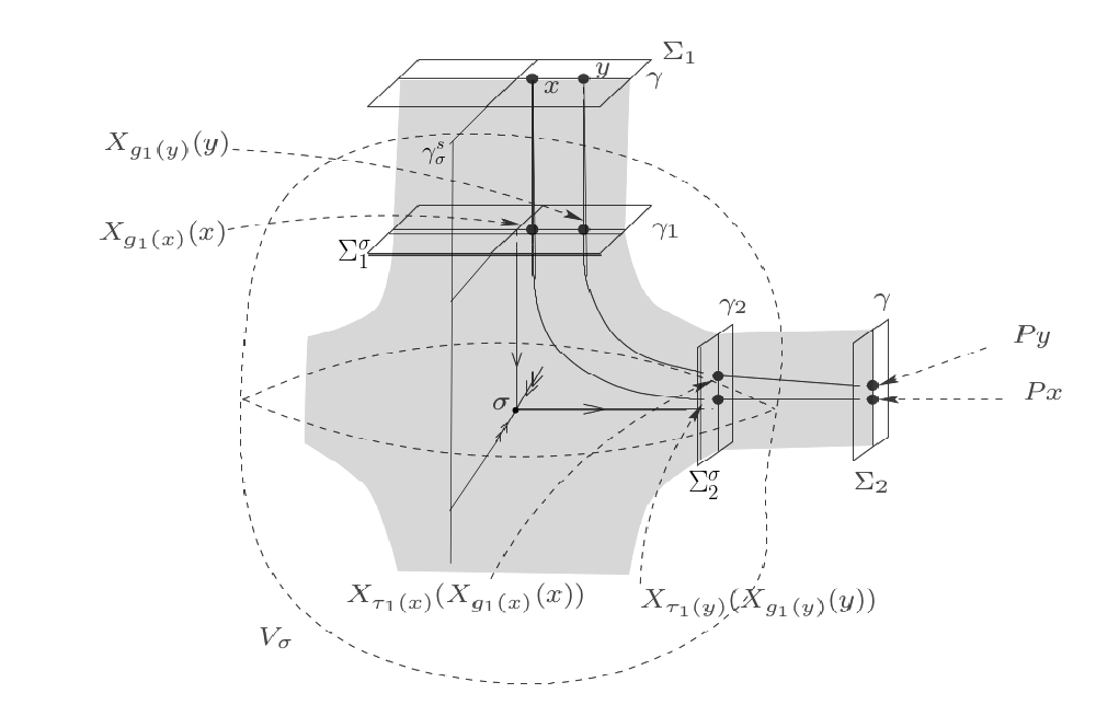
Figure 4. Linearization along a central-unstable surface on a neighborhood of a Lorenz-like singularity.

Because $g_{1}$ is $C^{2}$ we have that $|g_{1}(x)-g_{1}(y)|$ is bounded above by a constant times $|x-y|\leq|x-y|^{\alpha}$. It also follows that $|\tau_{1}(X_{g_{1}(x)}(x))-\tau_{1}(X_{g_{1}(y)}(y))|$ equals

$$(\lambda_{1})^{-1} \Big{|}\log\operatorname{dist}(X_{g_{1}(x)}(x),\gamma^{s}_{\sigma}\cap\gamma_{1})-\log\operatorname{dist}(X_{g_{1}(y)}(y),\gamma^{s}_{\sigma}\cap\gamma_{1})\Big{|}$$

$$\leq\displaystyle\frac{C_{0}|X_{g_{1}(x)}(x)-X_{g_{1}(y)}(y)|}{\min\{\operatorname{dist}(X_{g_{1}(x)}(x),\gamma^{s}_{\sigma}\cap\gamma_{1}),\operatorname{dist}(X_{g_{1}(y)}(y),\gamma^{s}_{\sigma}\cap\gamma_{1})\}}$$

for some constant $C_{0}>0$. Because $g_{1}$ is smooth and bounded, we have that the Poincaré map between $\gamma$ and $\gamma_{1}$ distorts distances by at most by a constant factor. Hence, we obtain $|X_{g_{1}(x)}(x)-X_{g_{1}(y)}(y)|\leq C_{0}|x-X_{g_{1}(x)-g_{1}(y)}(y)|\leq C_{0}|x-y|$ and $C_{0}\operatorname{dist}(X_{g_{1}(z)}(z),\gamma^{s}_{\sigma}\cap\gamma_{1})\geq\operatorname{dist}(z,\pi_{\gamma}(\Gamma))$. It follows that

$$|\tau_{1}(X_{g_{1}(x)}(x))-\tau_{1}(X_{g_{1}(y)}(y))|\leq C_{0}\dfrac{|x-y|}{\min\{\operatorname{dist}(x,\pi_{\gamma}(\Gamma)),\operatorname{dist}(y,\pi_{\gamma}(\Gamma))\}}.$$ (3.3)

Finally, using the expression of $P_{1}$ it follows that $g_{2}\circ P_{1}$ is $\alpha$-Hölder on $\gamma_{1}$, and so $|g_{2}(X_{\tau_{1}(x)}(X_{g_{1}(x)}(x)))-g_{2}(X_{\tau_{1}(y)}(X_{g_{1}(y)}(y)))|$ can be written

$$|g_{2}(P_{1}(X_{g_{1}(x)}(x)))-g_{2}(P_{1}(X_{g_{1}(y)}(y)))|\leq C_{1}|X_{g_{1}(x)}(x)-X_{g_{1}(y)}(y)|^{\alpha}\leq C_{2}|x-y|^{\alpha}$$ (3.4)

for come constants $C_{1},C_{2}>0$. Using the inequalities for $g_{1}$ together with (3.3) and (3.4), from (3.2) we arrive at the first inequality of the statement in the singular case as well. This completes the proof of the first inequality in the statement.

Now for the proof of the second inequality: in the case that $X_{[0,\tau(x)]}(x)$ never enters $V_{0}$, the result follows because $\tau|_{\Sigma_{1}}$ is of class $C^{2}$. Otherwise, $X_{[0,\tau(x)]}$ enters a neighborhood $V_{\sigma}$ of some singularity $\sigma\in S(\Lambda,X)$ and from (3.2) we write $D\tau(x)$ as

$$Dg_{1}(x)+D\tau_{1}(X_{g_{1}(x)}(x))DX_{g_{1}(x)}(x)+Dg_{2}(P_{1}(X_{g_{1}(x)}(x)))DP_{1}(X_{g_{1}(x)}(x))DX_{g_{1}(x)}(x).$$

Because $g_{1}$ and $g_{2}$ are $C^{2}$ and bounded on the $u$-curves where they are defined, we get that there exist a constant $C_{3}>0$ such that $|Dg_{1}|_{\infty}$, $|Dg_{2}|_{\infty}\leq C_{3}$. From the expression of $\tau_{1}$ we get that $D\tau_{1}(X_{g_{1}}(x))=\operatorname{dist}(X_{g_{1}(x)}(x),\gamma^{s}_{\sigma}\cap\gamma_{1})^{-1}\leq C_{4}\operatorname{dist}(x,{\mathcal{D}})^{-1}$. Identifying $P_{1}$ with $P_{1}(x_{1})=|x_{1}|^{-\lambda_{2}/\lambda_{1}}$ we have that $|DP_{1}(x_{1})|\leq C_{5}|x_{1}|^{\alpha-1}\leq|x_{1}|^{-1}$. Using this we get $|DP(X_{g_{1}(x)}(x))|\leq C_{6}\operatorname{dist}(X_{g_{1}(x)}(x),\gamma^{s}_{\sigma}\cap\gamma_{1})^{-1}\leq C_{6}C_{5}\operatorname{dist}(x,\pi_{\gamma}(\Gamma))^{-1}$ and the result follows. ∎

Remark 3.14 (Horizontal lines are $u$-curves).

We choose an identification $L:I\times B^{d_{s}}\to\Xi$ such that for all $c\in B^{d_{s}}$ the curve $\gamma_{i,c}:I_{i}\to\Sigma_{i}$ defined by $\gamma_{i,c}(t)=L(t,c)$ is a $u$-curve in $\Sigma_{i}$ for all $i=1,2,\dots,m$. In other words, with the identification given by $L$ we may assume that each horizontal line $\{(t,c):\ t\in I_{i}\}$ is a $u$-curve for all $c\in B^{d_{s}}$.

4. Properties of the one-dimensional quotient dynamics

We need some specific consequences of the construction and properties of the one-dimensional quotient map $f$ obtained in Section 3.

4.1. Topological properties of the one-dimensional dynamics

The following provides the existence of a special class of periodic orbits for $f$.

Proposition 4.1.

[15, Lemma 6.30] Let $f:\sum_{j}I_{j}\to I$ be a piecewise $C^{1}$ expanding map with finitely many branches $I_{1},I_{2}\dots,I_{m}$ such that each $I_{j}$ is a nonempty open interval, $|f^{\prime}|_{I_{j}}|\geq\sigma>2$ and $I\setminus(\sum_{j}I_{j})$ is finite. Then, for each small $\delta>0$ there exists $n=n(\delta)$ such that, for every nonempty open interval $J\subset\sum_{j}I_{j}$ with $|J|\geq\delta$, we can find $0\leq k\leq n$, a sub-interval $\widehat{J}$ of $J$ and $1\leq j\leq m$ satisfying

$$f^{k}|_{\widehat{J}}:\widehat{J}\to I_{j}\quad\text{is a diffeomorphism}.$$

In addition, $f$ admits finitely many periodic orbits $\mathcal{O}(p_{1}),\dots,\mathcal{O}(p_{k})$ contained in $\sum_{j}I_{j}$ with the property that every nonempty open interval $J\subset\sum_{j}I_{j}$ admits an open sub-interval $\widehat{J}$, a periodic point $p_{j}$ and an iterate $n$ such that $f^{n}|_{\widehat{J}}$ is a diffeomorphism onto a neighborhood of $p_{j}$.

Remark 4.2.

1. For the bidimensional map $F$ this shows that there are finitely many periodic orbits $\mathcal{O}(P_{1}),\dots,\mathcal{O}(P_{k})$ for $F$ so that $\pi(\mathcal{O}(P_{i}))=\mathcal{O}(p_{i}),i=1,\dots,k$, where $\pi:Q\to I$ is the projection on the first coordinate. Moreover, the union of the stable manifolds of these periodic orbits is dense in $Q$. See [15, Section 6.2] for details.

2. This also implies that the stable manifolds of the periodic orbits $P_{i}$ obtained above are dense in a neighborhood $U_{0}$ of $\Lambda$.

4.2. Exponential slow recurrence to the critical set

As a subtle consequence of Theorem 3.10 in [18] it was proved that the quotient map along stable leaves has exponentially slow recurrence to the critical/singular set ${\mathcal{D}}$ as follows.

Lemma 4.3.

[18, Theorem C] For each $\varepsilon>0$ we can find $\delta>0$ and $\xi>0$ so that

$$\limsup_{n\to\infty}\frac{1}{n}\log\operatorname{Leb}\left\{x\in I:\frac{1}{n}\sum_{j=0}^{n-1}-\log\operatorname{dist}_{\delta}(f^{j}(x),{\mathcal{D}})>\varepsilon\right\}<-\xi.$$ (4.1)

Remark 4.4.

Exponential slow recurrence implies a weaker condition: the slow recurrence to ${\mathcal{D}}$, that is, for all $\varepsilon>0$ there exists $\delta>0$ such that

$$\limsup_{n\to+\infty}\frac{1}{n}\sum^{n-1}_{j=0}-\log\operatorname{dist}_{\delta}(f^{j}(x),{\mathcal{D}})\leq\varepsilon\ \text{for}\ \operatorname{Leb}-a.e.\ x\in I.$$ (4.2)

4.3. Ergodic properties of $f$

The map $f$ is piecewise expanding with Hölder derivative which enables us to use strong results on one-dimensional dynamics.

4.3.1. Existence and finiteness of acim’s

It is well-known [33] that $C^{1}$ piecewise expanding maps $f$ of the interval such that $1/|f^{\prime}|$ has bounded variation have absolutely continuous invariant probability measures whose basins cover Lebesgue almost all points of $I$.

Using an extension of the notion of bounded variation this result was extended in [34] to $C^{1}$ piecewise expanding maps $f$ such that $1/|f^{\prime}|$ is $\alpha$-Hölder for some $\alpha\in(0,1)$. In addition, from [34, Theorem 3.3], there are finitely many ergodic absolutely continuous invariant probability measures $\upsilon_{1},\dots,\upsilon_{l}$ of $f$ and every absolutely continuous invariant probability measure $\upsilon$ decomposes into a convex linear combination $\upsilon=\sum_{i=1}^{l}a_{i}\upsilon_{i}$. From [34, Theorem 3.2] considering any subinterval $J\subset I$ and the normalized Lebesgue measure $\operatorname{Leb}_{J}=(\operatorname{Leb}|_{J})/\operatorname{Leb}(J)$ on $J$, every weak^∗ accumulation point of $n^{-1}\sum_{j=0}^{n-1}f_{*}^{j}(\operatorname{Leb}_{J})$ is an absolutely continuous invariant probability measure $\upsilon$ for $f$ (since the characteristic function of $J$ is of generalized $1/\alpha$-bounded variation). Hence, the basins of the $\upsilon_{1},\dots,\upsilon_{l}$ cover $I$ Lebesgue modulo zero: $\operatorname{Leb}\big{(}I\setminus(B(\upsilon_{1})+\dots+B(\upsilon_{l})\big{)}=0.$ Note that from [34, Lemma 1.4] we also know that the density $\varphi$ of any absolutely continuous $f$-invariant probability measure is bounded from above.

4.3.2. Absolutely continuous measures and periodic orbits

Now we relate some topological and ergodic properties.

Lemma 4.5.

[18, Lemma 2.12] For each periodic orbit $\mathcal{O}(p_{i})$ of $f$ given by Proposition 4.1, there exists a unique ergodic absolutely continuous $f$-invariant probability measure $\upsilon_{j}$ such that $p_{i}\in\operatorname{int}(\operatorname{supp}\upsilon_{j})$, and vice-versa.

4.4. Consequences for the flow dynamics in the trapping region

Combining the previous properties we can deduce the following useful result.

Theorem 4.6.

[18, Theorem 2.14] The union of the stable manifolds of the singularities in a non-trivial connected singular-hyperbolic attracting set $\Lambda$ is dense in the topological basin of attraction, that is $U_{0}\subset\overline{\bigcup_{\sigma\in S(X,\Lambda)}W^{s}(\sigma)}.$

This in particular implies the following.

Proposition 4.7.

The support of every ergodic physical measure of a non-trivial connected singular-hyperbolic attracting set contains some Lorenz-like singularity.

Proof.

Arguing by contradiction, let $\mu$ be an ergodic physical measure such that $\operatorname{supp}(\mu)$ does not contain any Lorenz-like singularity. Hence it does not contain any singularity by Remark 1.6(3).

Therefore, $\Lambda_{0}=\operatorname{supp}(\mu)$ is a uniformly hyperbolic transitive subset (by Theorem 1.3) and unstable manifolds are well-defined and contained in $\Lambda_{0}$; see e.g. [44]. Thus $\Lambda_{0}$ is a connected hyperbolic attractor which is a closed and open subset of $\Lambda$; see e.g. [43]. By connectedness of $\Lambda$ we must have $\Lambda_{0}=\Lambda$. This contradicts the non-trivial assumption on $\Lambda$. ∎

4.5. Construction of an induced piecewise expanding Markov map for the one-dimensional quotient transformation

Here we explain how to obtain a $C^{1+\alpha}$ expanding map induced by $f$ with inducing time having exponential tail, as defined in Subsection 2.1.1, for each $f$-invariant ergodic absolutely continuous probability measure. A general reference containing the main results and complete detailed proofs is [1].

4.5.1. Hyperbolic times

Let $B>1$ and $\beta$ be as in the non-degeneracy conditions (C1) and (C2). Let $0<\sigma<1$, $0<b<1/2$ and $\delta>0$. We say that a natural number $n$ is a $(\sigma,\delta)$-hyperbolic time for $x\in I$ if for all $1\leq k\leq n$, we have

$$|(f^{k})^{\prime}(f^{n-k}(x))|\geq\sigma^{-k}\ \ \ \text{and}\ \ \ \operatorname{dist}_{\delta}{(f^{n-k}(x),{\mathcal{D}})}\geq\sigma^{kb}.$$

Lemma 4.8.

[2, Lemma 5.2 & Corollary 5.3] Given $\sigma\in(0,1)$ and $\delta>0$, there exist $\delta_{1},D_{1}$ (depending only on $\sigma,\delta$ and on the map $f$) such that for any $x\in I$ and $n\geq 1$ a $(\sigma,\delta)$-hyperbolic time for $x$, there exists an open interval $V_{n}(x)$ containing $x$ with the following properties:

1. $f^{n}$ maps $V_{n}(x)$ diffeomorphically onto the interval $(f^{n}(x)-\delta_{1},f^{n}(x)+\delta_{1})$;

2. for $1\leq k<n$ and $y,z\in V_{n}(x)$, $|f^{n-k}(y)-f^{n-k}(z)|\leq\sigma^{k/2}|f^{n}(y)-f^{n}(z)|$;

3. $f^{n}$ has distortion bounded by $D_{1}$ on $V_{n}(x)$, that is, $|(f^{n})^{\prime}(y)|/|(f^{n})^{\prime}(z)|\leq D_{1}$, for all $y,z\in V_{n}(x)$;

4. $V_{n}(x)\subset(x-2\delta_{1}\sigma^{n},x+2\delta_{1}\sigma^{n})$.

The sets $V_{n}(x)$ in the last lemma are called hyperbolic pre-intervals and their images $f^{n}(V_{n}(x))$ are called hyperbolic intervals.

Lemma 4.9.

([2, Lemma 5.4] and [16, Lemma 1.8]) There exist $\theta>0$ and $0<\delta<1$ (depending only on $f$ and on its expanding rate) such that, for Lebesgue almost every $x\in I$, we can find $n_{0}\geq 1$ satisfying: for each $n>n_{0}$ there are $(\sigma,\delta)$-hyperbolic times $1\leq n_{1}<\cdots<n_{l}\leq n$ for $x$ with $l\geq\theta n$. Moreover, each hyperbolic time $n_{i}$ satisfies

$$\sum_{j=n_{i}-k}^{n_{i}-1}\log\operatorname{dist}_{\delta}(f^{j}(x),{\mathcal{D}})\geq bk\log\sigma,\ \text{for all }0\leq k\leq n_{i},\ 1\leq i\leq l.$$ (4.3)

4.5.2. Inducing the one-dimensional map

We have all the conditions to perform the construction of an induced map from $f$ as in [4, Main Theorem 1].

Let $\delta_{1}$ be given by Lemma 4.8. For each $f$-invariant ergodic absolutely continuous probability measure $\nu$, we fix a point $p\in\operatorname{int}(\operatorname{supp}\nu)$ and an integer $N\geq 1$ such that $\cup^{N}_{j=0}f^{-j}(p)$ is $\delta_{1}/3$-dense in $\operatorname{supp}\nu$ and does not contain any element of ${\mathcal{D}}$.

Theorem 4.10.

[3, 19, 32] There exists a neighborhood $\Delta\subset\operatorname{int}(\operatorname{supp}\nu)\setminus{\mathcal{D}}$, a countable Lebesgue modulo zero partition $\mathcal{P}$ of $\Delta$ into sub-intervals; a function $R:\Delta\to{\mathbb{N}}$ defined almost everywhere, constant on elements of the partition $\mathcal{P}$; and constants $C>0$, $0<\rho<1$ such that, for all $J\in\mathcal{P}$ and $R=R(J)$, the map $F:=f^{R}:J\to\Delta$ is a $C^{1+\alpha}$ diffeomorphism, satisfies the bounded distortion property and is uniformly expanding: for each $x,y\in J$

$$\left|\frac{F^{\prime}(x)}{F^{\prime}(y)}-1\right|\leq C|F(x)-F(y)|^{\alpha}\quad\text{and}\quad|F(x)-F(y)|>\rho^{-1}|x-y|.$$

Moreover, for each $J\in\mathcal{P}$ there exists $0<k\leq N$ such that $n:=R(J)-k$ is a $(\sigma,\delta_{1})$-hyperbolic time for each $x\in J$; $J\subset V_{n}(x)$ and, in addition, there is some $\delta>0$ such that $\operatorname{dist}(f^{j}(J),{\mathcal{D}})\geq\delta$ for all $n\leq j<R(J)$.

Remark 4.11.

Without loss of generality we assume that $\rho<\sigma$ and use $\sigma^{-1}$ as the expansion rate for $F$. Making $\delta_{!}$ smaller if necessary, we can take $\delta=\delta_{1}$ and we may assume that $R(J)$ is a $(\sigma,\delta_{1})$-hyperbolic time for all $x\in J$ (instead of $R(J)-k$), because the map $f$ is expanding and the iterates $f^{j}(J)$ are $\delta$-distant from ${\mathcal{D}}$. From now on we make this assumption.

Let $\mathcal{P}^{(n)}=\bigvee^{n-1}_{j=0}F^{-j}(\mathcal{P})$ and denote by $\mathcal{P}^{(n)}(x)$ the element of the partition $\mathcal{P}^{(n)}$ that contains $x$. Letting $R_{n}(x)=\sum_{j=0}^{n-1}R(F^{j}(x))$ we get that $F^{n}(x)=f^{R_{n}(x)}(x)$. It follows from Theorem 4.10 that, for all $x,y\in\Delta$ such that $y\in\mathcal{P}^{(n)}(x)$

$$|F^{n}(x)-F^{n}(y)|\geq\sigma^{-(R_{n}(x)-j)}|f^{j}(x)-f^{j}(y)|,\ j=0,1,\dots,R_{n}(x)-1,$$ (4.4)

and since $R_{n}(x)$ is a $(\sigma,\delta_{1})$-hyperbolic time for every $y\in\mathcal{P}^{(n)}(x)$

$$\operatorname{dist}(f^{j}(y),{\mathcal{D}})\geq\sigma^{b(R_{n}(x)-j)},\ j=0,1,\dots,R_{n}(x)-1.$$ (4.5)

4.6. The $C^{1}$ expanding semiflow

Now we check the conditions (3) and (4) from Subsection 2.1 to obtain an expanding semiflow associated to each ergodic absolutely continuous $f$-invariant probability measure.

4.6.1. The induced roof function

Let $r:\Delta\to{\mathbb{R}}$ be defined as $r(x)=\sum^{R(x)-1}_{j=0}\tau(f^{j}(x)),$ for all $x\in\Delta$. Next we prove that $r$ satisfies condition (3) of Subsection 2.1.1.

Lemma 4.12.

For all $h\in\mathcal{H}$ it holds that $|(r\circ h)^{\prime}|_{\infty}<+\infty.$

Proof.

Let $h\in\mathcal{H}$, $h:\Delta\to J$ be an inverse branch for $F=f^{R}$ with inducing time $\ell=R(J)$. Fixing $x\in J$, we have

$$|(r\circ h)^{\prime}(x)|=\frac{|r^{\prime}(h(x))|}{|F^{\prime}(h(x))|}=\left|\displaystyle\sum^{\ell-1}_{j=0}\frac{(\tau^{\prime}\circ f^{j})\cdot(f^{j})^{\prime}}{F^{\prime}}\circ h(x)\right|.$$

By Lemma 3.13 and the fact that $\ell$ is a hyperbolic time for all $x\in J$ we have that $|\tau^{\prime}(f^{j}(h(x)))|\leq C\operatorname{dist}(f^{j}(h(x)),{\mathcal{D}})^{-1}\leq C\sigma^{-(\ell-j)b}$, for some constant $C>0$ and for all $j=0,1,\dots,\ell-1.$ It follows from inequality (4.4) that $|(f^{j})^{\prime}/F^{\prime}|\circ h(x)\leq\sigma^{\ell-j}$. Hence $|(r\circ h)^{\prime}(x)|\leq C\sum^{\ell-1}_{j=0}\sigma^{-(\ell-j)b}\cdot\sigma^{\ell-j}\leq C\sum_{j=0}^{\infty}\sigma^{(1-b)j}<\infty.$ ∎

For each $x\in\Delta$ and $\varepsilon,\delta>0$ we define the recurrence time of $x$ by

$${\mathcal{R}}(x)={\mathcal{R}}_{\varepsilon,\delta}(x)=\min\left\{N\geq 1:\,\dfrac{1}{N}\sum^{N-1}_{j=0}-\log\operatorname{dist}_{\delta}(f^{j}(x),{\mathcal{D}})\leq 2\varepsilon\right\}.$$

The slow recurrence given by the Lemma 4.3 can be translated as: for all $\varepsilon>0$, there exists $\delta>0$ such that $\limsup_{n\to+\infty}\frac{1}{n}\log\operatorname{Leb}(\{x\in I:\,{\mathcal{R}}(x)>n\})<0.$ We say that the sets $\{x\in I:\,{\mathcal{R}}(x)>n\}$ are the tail of hyperbolic times. Hence, the tail of hyperbolic times converges exponentially fast to zero. In [32] the construction of the induced Markov map from [3] was improved so that the tail of $R$ converges to zero at the same speed as the tail of hyperbolic times. In particular, in the same setting of Theorem 4.10, the inducing time function $R$ has exponential tail.

Proposition 4.13.

There exist constants $c,C>0$ such that for all $n\geq 1$

$$\operatorname{Leb}(\{x\in\Delta:R(x)>n\})\leq Ce^{-cn}.$$

Remark 4.14.

Recently a similar result has been stated in [30] under weaker assumptions.

It follows from Proposition 4.13 that

Proposition 4.15.

The function $r$ has exponential tail.

Proof.

Fixed $J\in\mathcal{P}$, using inequality (4.3) of Lemma 4.9 and the fact that $\tau$ has logarithmic growth (item (1a) of Theorem 3.10) we get

$$r(x)=\sum_{j=0}^{R(x)-1}\tau(f^{j}(x))\leq\sum_{j=0}^{R(x)-1}-\log\operatorname{dist}_{\delta}(f^{j}(x),{\mathcal{D}})\leq-bR(x)\log\sigma.$$

Thus, there exists constants $C,\tilde{c}>0$ such that $\operatorname{Leb}(\{x\in\Delta:\ r(x)>n\})\leq Ce^{-\tilde{c}n}$. Using the bounded distortion of $F^{\prime}$ is straightforward to get that $r$ satisfies the exponential tail condition as stated in Subsection 2.1.2. ∎

4.7. $C^{1+}$ skew product semiflow

Now we note that from Theorem 3.10 we already have all that is needed to obtain a $C^{1+}$ skew product semiflow, with the exception of the UNI condition (5), which we focus on the Subsection 5.1.

Indeed, let $\widehat{\Delta}=\cup_{x\in\Delta}W^{s}_{x}$ and define $\widehat{F}:\widehat{\Delta}\to\widehat{\Delta}$ by $\widehat{F}(x)=P^{R(x)}(x)$ and the suspension semiflow $\widehat{F}_{t}:\widehat{\Delta}^{r}\to\widehat{\Delta}^{r}$ with base map $\widehat{F}$ and roof function $r$.

Through the identification of $\widehat{\Delta}$ with $\Delta\times B^{d_{s}}$, it follows from item 4 of Theorem 3.10 that $\widehat{F}_{t}$ satisfies condition (4) of a hyperbolic skew product semiflow, from Subsection 2.1.

5. Exponential mixing for singular-hyperbolic attracting sets

Throughout this section we denote by ${\mathfrak{X}}^{s}_{dsh}(M)$ the subset of ${\mathfrak{X}}^{s}(M)$ that admits a $2$-strong dissipative singular-hyperbolic attracting set, $s\geq 1$.

Here we construct a $C^{2}$ open subset $\mathcal{U}\subset{\mathfrak{X}}^{2}_{dsh}(M)$ where the UNI condition holds. This enable us to construct a suspension semiflow with exponential decay of correlations as in Theorem 2.4.

We also prove Theorem 2.5 showing that smooth observables for the original flow lie on the right function spaces when composed with the conjugacy.

Finally, we finish the section by deducing the exponential convergence to the equilibrium for the original flow. This is a by product of all the work made to prove exponential decay of correlations for the physical measures.

5.1. The UNI condition after small perturbations

In this section we construct an open and dense subset $\mathcal{U}$ of ${\mathfrak{X}}^{2}_{dsh}(M)$ where all vector fields have a roof function that satisfies the UNI condition. In particular, we construct a family of suspension semiflows, one for each ergodic physical measure of the attracting set, which satisfy the conditions of Theorem 2.4 and we get exponentially mixing for them.

Recall that there exists a one-to-one correspondence between the periodic points of the Poincaré map and its quotient along the stable leaves.

Lemma 5.1.

A point $x\in I$ is periodic for $f$ if and only if there exists a periodic point $z\in\pi^{-1}(x)$ for the Poincaré map $P$.

Remark 5.2.

Using Lemma 5.1, from now on we make no distinction between a periodic point of the Poincaré map and its quotient along stable leaves.

Since the strong dissipative condition is open in the $C^{1}$ topology and singular-hyperbolic attracting sets persist by $C^{1}$-small perturbations of the vector field, we have that ${\mathfrak{X}}^{s}_{dsh}(M)$ is open in ${\mathfrak{X}}^{s}(M)$ (with the $C^{s}$ topology), for all $s\geq 1$.

For a vector field $X\in{\mathfrak{X}}^{2}_{dsh}(M)$ we can repeat the constructions of Chapter 3. We need to perform the constructions for more than one vector field so, where necessary, we make the dependence on the vector field explicit in what follows. For instance, $P_{X}:\Xi\backslash\Gamma_{X}\to\Xi_{X}$ denotes the Poincaré map of $X$ with Poincaré time given by $\tau_{X}$; and $f_{X}:I\setminus{\mathcal{D}}\to I$ is the corresponding one-dimensional quotient map.

Definition 5.3.

Let $\Lambda$ be a singular-hyperbolic attracting set for $X\in{\mathfrak{X}}^{2}_{dsh}(M)$. Let $P:\Xi\backslash\Gamma\to\Xi$ and $f:I\backslash{\mathcal{D}}\to I$ be the global Poincaré map and its quotient along stable leaves, respectively, for $X$ as in Subsection 3.2.

We say that $X$ satisfies the UNI condition if, for each ergodic physical measure $\mu$ of $X$ corresponding to an ergodic physical measure $\hat{\nu}$ of $P$ given by an ergodic $f$-invariant absolutely continuous probability measure $\nu$, there exists an open interval $\Delta\subset\operatorname{int}(\operatorname{supp}\nu)\subset I$ and an induced function $R:\Delta\to{\mathbb{N}}$ (as in Theorem 4.10) such that the induced roof function $r:\Delta\to{\mathbb{R}}$ given by $r(x)=\sum^{R(x)-1}_{j=0}\tau(f^{j}(x))$ satisfies the UNI condition.

Let us fix an ergodic physical measure $\hat{\nu}$ for $P$ and $\nu$ for $f$. Letting $F=f^{R}:\Delta\to\Delta$ be an induced full branch Markov map constructed for $X\in{\mathfrak{X}}^{2}(M)$ in Theorem 4.10, for a function $\varphi:\Delta\to{\mathbb{R}}$ and $n\geq 1$ we denote $S^{F}_{n}\varphi=\sum^{n-1}_{j=0}\varphi\circ F^{j}$.

Now we describe the open set $\mathcal{U}$ where Theorem 2.5 holds. We set $\mathcal{U}$ to be the subset of vector fields in ${\mathfrak{X}}^{2}_{dsh}(M)$ such that, for all $X\in\mathcal{U}$, each physical measure $\nu$ of $f$ and each corresponding induced Markov map $F:\Delta\to\Delta$, there exist two distinct periodic points $x_{1},x_{2}\in\Delta\subset\operatorname{int}(\operatorname{supp}\nu)$ for the induced Markov map $F$ with the same period $p$ and satisfying:

1. the orbits are distinct; and they visit the interior of the same elements of the partition $\mathcal{P}$ the same number of times as the other, but necessarily in some different order to each other; and

2. $S^{F}_{p}r(x_{1})\neq S^{F}_{p}r(x_{2})$.

Lemma 5.4.

The vector fields in $\mathcal{U}$ satisfy the UNI condition.

Proof.

Let $X\in\mathcal{U}$ and assume that $X$ does not satisfies the UNI condition. Then, there exist an ergodic $f$-invariant absolutely continuous probability measure $\nu$, an induced map $F:\Delta\to\Delta$ with $\Delta\subset\operatorname{int}(\operatorname{supp}\nu)$, a $C^{1}$ function $\varphi:\Delta\to{\mathbb{R}}$ and a function $\psi:\Delta\to{\mathbb{R}}$ constant on elements of the induced partition $\mathcal{P}$ of $\Delta$ such that $r=\psi+\varphi\circ F-\varphi$.

Let $x_{1},x_{2}\in\Delta$ be two periodic points with period $p$ for the induced Markov map $F$ satisfying conditions (i) - (ii) of the definition of $\mathcal{U}$. It follows that $S^{F}_{p}r(x_{i})=S^{F}_{p}\psi(x_{i})$. Since $\psi$ is constant on elements of the partition $\mathcal{P}$, by condition (ii) above, we get that $S^{F}_{p}\psi(x_{1})=S^{F}_{p}\psi(x_{2})$. This is a contradiction with $S^{F}_{p}r(x_{1})\neq S^{F}_{p}r(x_{2})$. ∎

The proofs of the next two propositions follow the steps presented in [20]. In Proposition 5.5 we show that, if we start with a vector field $X\in{\mathfrak{X}}^{2}_{dsh}(M)$ that does not satisfy the UNI condition and change slightly the velocity of a well chosen periodic orbit, then the new vector field satisfies the UNI condition and is arbitrarily $C^{2}$-close to the initial vector field $X$. In particular, we get that the subset of vector fields in ${\mathfrak{X}}^{2}_{dsh}(M)$ that satisfies the UNI condition is dense in the $C^{2}$ topology. In Proposition 5.7, we show that the inequality that we obtained in the previous propostion remains valid for vector fields $C^{2}$-close to $X\in\mathcal{U}$.

Proposition 5.5.

The set $\mathcal{U}$ is $C^{2}$-dense in ${\mathfrak{X}}^{2}_{dsh}(M)$: for each $X\in{\mathfrak{X}}^{2}_{dsh}(M)$ there exists $\delta>0$ and a $\delta$-$C^{2}$-close vector field $Y\in\mathcal{U}$ which is a multiple of $X$.

In other words, any $X\in{\mathfrak{X}}^{2}_{dsh}(M)$ admits a time reparametrization which lies in $\mathcal{U}$.

Proof.

Let $X\in{\mathfrak{X}}^{2}_{dsh}(M)$ and assume that $X$ does not satisfy the UNI condition. Hence, there exist an ergodic $f_{X}$-invariant absolutely continuous probability measure $\nu$, an induced map $F_{X}:\Delta_{X}\to\Delta_{X}$ with $\Delta_{X}\subset\operatorname{int}(\operatorname{supp}\nu)$, a $C^{1}$ function $\varphi:\Delta\to{\mathbb{R}}$, and a function $\psi:\Delta_{X}\to{\mathbb{R}}$ constant on elements of the partition $\mathcal{P}_{X}$ together with $\varphi:\Delta_{X}\to{\mathbb{R}}$ of class $C^{1}$ such that $r_{X}=\psi+\varphi\circ F_{X}-\varphi$.

Let $x_{1}$ and $x_{2}$ be two periodic points with the same period $p$ for the map $F_{X}$. We may assume without loss of generality, because $F_{X}$ is a full branch Gibbs-Markov map, that the orbits are distinct and visit the same elements of the partition $\mathcal{P}_{X}$ the same number of times as the other, but in a different order. If $J_{1},J_{2}$ are two disjoint elements of the partition $\mathcal{P}_{X}$, we can choose the period $p=4$, $x_{1}$ and $x_{2}$ such that

$$x_{1},F_{X}(x_{1})\in J_{1},F_{X}^{2}(x_{1}),F_{X}^{3}(x_{1})\in J_{2}\quad\text{and}\quad x_{2},F_{X}^{2}(x_{2})\in J_{1},F_{X}(x_{2}),F_{X}^{3}(x_{2})\in J_{2}.$$

Note that $S^{F_{X}}_{p}r(x_{1})=S^{F_{X}}_{p}\psi(x_{1})=S^{F_{X}}_{p}\psi(x_{2})=S^{F_{X}}_{p}r(x_{2})$ since $x_{1}$ and $x_{2}$ visit the same elements of $\mathcal{P}_{X}$ an equal number of times and $\psi$ is constant on each element of $\mathcal{P}_{X}$. We have that $S^{F_{X}}_{p}r(x_{i})$ is a multiple of the period of $x_{i}$ with respect to the flow of $X$, and does not depends on the functions $\varphi$ and $\psi$. Indeed

$$S^{F_{X}}_{4}r(x_{i})=\sum^{3}_{j=0}r(F_{X}^{j}(x_{i}))=\sum^{3}_{j=0}\sum^{R(F_{X}^{j}(x_{i}))-1}_{k=0}\tau(f_{X}^{k}(F_{X}^{j}(x_{i})))=\sum^{R_{4}(x_{i})-1}_{k=0}\tau(f^{k}(x_{i}))$$ (5.1)

Because $F_{X}^{4}(x_{i})=x_{i}$, it follows that $f_{X}^{R_{4}(x_{i})}(x_{i})=x_{i}$. Letting $t_{0}=S^{F_{X}}_{4}r(x_{i})$ and using (5.1), we have $X_{t_{0}}(x_{i})=x_{i}$ (recall the convention that we are using for periodic points on Remark 5.2). Hence, it follows that $t_{0}$ is a multiple of the period of $x_{1}$ and $x_{2}$ by the action of the flow.

We modify the roof function $\tau_{X}:\Xi\to{\mathbb{R}}^{+}$ in a small neighborhood of $x_{2}$ that does not intersect the orbit of $x_{1}$ to ensure that the induced roof function $r_{X}$ satisfies $S^{F_{X}}_{p}r(x_{1})>S^{F_{X}}_{p}r(x_{2})$. Let $V_{0}$ and $V_{1}$ be open small neighborhoods of $x_{2}$ that do not intersect the orbit of $x_{1}$ with $\overline{V_{0}}\subsetneq V_{1}$ and consider a $C^{\infty}$ bump function $\xi:M\to[0,1]$ such that $\xi|_{V_{0}}\equiv 1$ and $\xi_{M\backslash V_{1}}\equiv 0$. For all $\delta>0$ define the vector field $X_{\delta}=X+\delta\xi X$ which is $\delta$-close to $X$ in the $C^{1}$-topology. Inside $V_{0}$ the vector field $X_{\delta}$ is equal to $(1+\delta)X$ and outside of $V_{1}$ it equals $X$. Thus $x_{2}$ is still a periodic orbit for $X_{\delta}$ but with a smaller period than before. Thus, he have that $S^{F_{X_{\delta}}}_{4}r(x_{1})>S^{F_{X_{\delta}}}_{4}r(x_{2})$ as we desired.

Now it follows from Lemma 5.4 that $X_{\delta}$ satisfies the UNI condition. Moreover $\|X-X_{\delta}\|_{2}=\delta\|\xi X\|_{2}$ and so we can make the perturbation arbitrarily close to the original vector field in $C^{2}$ topology. ∎

Remark 5.6.

If we start with a $C^{s}$ vector field, for some $s\geq 2$, then the same argument gives a $\delta$-$C^{s}$-close vector field $X_{\delta}\in\mathcal{U}$.

Proposition 5.7.

The set $\mathcal{U}$ is $C^{2}$-open in ${\mathfrak{X}}^{2}_{dsh}(M)$.

Proof.

Let $X\in\mathcal{U}$ and for a fixed ergodic physical measure, let $x_{1},x_{2}\in\Delta_{X}$ as conditions (i)-(ii) of the definition of $\mathcal{U}$ above. We are going to show that these conditions persist for all $C^{2}$-close enough vector fields $Y$. Since we have only finitely many ergodic physical measures supported on the attracting set $\Lambda$ of $X$, it is enough to argue for one such ergodic physical measure.

Let $L\geq 1$ be big enough so that $\mathcal{O}_{F_{X}}(x_{i})\subset\{x\in M:\ R_{X}(x)\leq L\}$, for $i=1,2$. Recall that because $x_{1},x_{2}$ are also periodic points for $X$ inside a singular-hyperbolic attracting set, then they are hyperbolic periodic orbits of saddle type and admit smooth continuations to all $C^{1}$ nearby vector fields $Y$.

Because the construction of the induced Markov map from the one-dimensional map is made outside a neighborhood of the critical/singular set, we can also control the distance of $F_{X}|_{\{R_{X}\leq L\}}$ and $F_{Y}|_{\{R_{Y}\leq L\}}$ (since we are only working with finitely many iterates of the maps $f_{X}$ and $f_{Y}$). Moreover, because the construction is inductive, in each step of the construction we can ensure that the open intervals of the partition $\mathcal{P}_{X}$ inside $\{R_{X}\leq L\}$ are arbitrarily close to their correspondent open intervals of $\mathcal{P}_{Y}$ inside $\{R_{Y}\leq L\}$. (To keep all the ingredients of the inductive construction preserved by $Y$ here, we need $Y$ and $X$ to be $C^{2}$-close. For example, this is needed to control the size of the hyperbolic balls. Check the outline of the construction in Section 4.5 and for more details check [3, Sections 3 and 4] and [20]).

Thus, we have that the continuation $y_{i}$ of $x_{i}$, $i=1,2$, for vector fields $Y$ close to $X$ has the same combinatorics as before, that is, $y_{1}$ and $y_{2}$ has the same period $p$ and visit the same elements of the partition $\mathcal{P}_{Y}$ with respect to the map $F_{Y}$. Finally, because $S^{F_{Y}}_{p}r_{Y}(y_{1})$ is a multiple of the period of $y_{1}$ for $Y$, we have that $S^{F_{Y}}_{p}r_{Y}(y_{1})\neq S^{F_{Y}}_{p}r_{Y}(y_{2})$. Now it follows that $r_{Y}$ cannot be written as $r_{Y}=\psi_{Y}+\varphi_{Y}\circ F_{Y}-\varphi_{Y}$ with $\psi_{Y}:\Delta_{Y}\to{\mathbb{R}}$ constant on elements of the partition $\mathcal{P}_{Y}$ and $\varphi_{Y}:\Delta_{Y}\to{\mathbb{R}}$ with class $C^{1}$, otherwise following the same argument of the Proposition 5.5 we would get that $S^{F_{Y}}_{p}r_{Y}(y_{1})=S^{F_{Y}}_{p}r_{Y}(y_{2})$. ∎

5.2. Proof of the main technical result

Here we prove Theorem 2.5.

We show that the original flow is semiconjugated to a suspension semiflow $\widehat{F}_{t}$ and that, given observables with certain amount of regularity for the original flow, we get observables in the right space for the suspension semiflow, and the measure in the original flow is the pushforward of the measure for the suspension semiflow. This provides what is needed to transfer the results about decay of correlations from the suspension semiflow to the original flow.

Let $X\in\mathcal{U}$ and for each ergodic physical measure supported on the attracting set, let $F:\Delta\to\Delta$ be the induced Markov map for $X$ with inducing function given by $R$ and roof function given by $r(x)=\sum^{R(x)-1}_{j=0}\tau(P^{j}(x))$, as before. We consider also $\widehat{\Delta}=\cup_{x\in\Delta}W^{s}_{x}$ and $\widehat{F}:\widehat{\Delta}\to\widehat{\Delta}$ defined by $\widehat{F}(x)=P^{R(x)}(x)$ together with the suspension semiflow $\widehat{F}_{t}:\widehat{\Delta}^{r}\to\widehat{\Delta}^{r}$.

Using the identification of $\widehat{\Delta}$ with $\Delta\times B^{d_{s}}$, it follows that $\widehat{F}_{t}$ and $\mu^{r}_{\widehat{F}}$ satisfy Theorem 2.4, that is, we have exponentially fast decay of correlations in the function spaces $C^{\alpha}_{\text{loc}}(\widehat{\Delta}^{r})$ and $C^{\alpha,2}_{\text{loc}}(\widehat{\Delta}^{r})$ for the skew product semiflow associated to each physical measure of the global Poincaré return map.

5.2.1. From the suspension flow to the original flow

The harder part of Theorem 2.5 is item (ii). We obtain this using a Hölder bound on the semiconjugation between the skew product semiflow and the original flow, given by Theorem 5.8. In the rest of the section we prove this bound.

From now on we work with a fixed vector field $X\in\mathcal{U}$ and a fixed ergodic physical measure and its corresponding skew product semiflow.

The next result enables us to pass from the ambient manifold ${\mathbb{R}}^{N}$ using the map $p:\widehat{\Delta}^{r}\to{\mathbb{R}}^{N}$ given by $p(x,y,u)=X_{u}(x,y)$.

Theorem 5.8.

There is a constant $C>0$ so that for all $(x_{1},y_{1},u_{1}),(x_{2},y_{2},u_{2})\in\widehat{\Delta}^{r}$, we have $|p(x_{1},y_{1},u_{1})-p(x_{2},y_{2},u_{2})|\leq C(|F(x_{1})-F(x_{2})|^{\alpha}+|y_{1}-y_{2}|+|u_{1}-u_{2}|).$

Remark 5.9.

The map $p$ cannot be Hölder with globally bounded Hölder constant since the expansion rate of $F$ is unbounded over all the atoms of the induced partition. This detail, which demands the extension of the space of admissible observables, was missed in previous works on exponential mixing for singular-hyperbolic attracting sets.

Proof of Theorem 2.5.

1. The semiconjugacy property follows directly from the definition of $p$ and of the skew product semiflow.

   For the push-forward property, it is enough to check that $p_{*}\mu^{r}_{\widehat{F}}$ is an ergodic physical measure for $X_{t}$ and use the finiteness of such measures and the decomposition of any physical measure provided by item 3 of Theorem 1.8. By construction of $\mu_{\widehat{F}}$ we have that this measure is a ergodic physical measure for the map $\widehat{F}$ (consult [17, Subsection 6.2]). Using the same arguments of [17, Subsection 6.4] it follows that $\mu^{r}_{\widehat{F}}$ is a physical measure for the suspension flow $\widehat{F}$. Using the fact that $p$ is a semiconjugacy between $\widehat{F}_{t}$ and $X_{t}$, it follows that $p(B(\mu^{r}_{\widehat{F}}))\subset B(p_{*}\mu^{r}_{\widehat{F}})$. Since $p$ is a local diffeomorphism it follows that $B(p_{*}\mu^{r}_{\widehat{F}})$ has positive Lebesgue measure. Hence $p_{*}\mu^{r}_{\widehat{F}}$ is an ergodic invariant physical probability measure for $X$ supported in $U_{0}$, and so in $\Lambda$. It follows that $p_{*}\mu^{r}_{\widehat{F}}=\mu_{i}$ for some ergodic physical measure supported on $\Lambda$.

2. The result follows from Theorem 5.8 and successive use of the Mean Value Inequality Theorem.

∎

We are left to prove Theorem 5.8 in what follows.

5.2.2. Proof of the Hölder estimate

In the next lemma, given the Poincaré time function $\tau$ for $X$, we denote $\tau_{k}(x)=\sum^{k-1}_{j=0}\tau(P^{j}(x))$, for all $x\in\Xi\backslash\Gamma$. Also recall that $\tau$ is constant on each stable leaf, so $\tau(x)=\tau(\pi(x))$ for all $x\in\Xi\backslash\Gamma$.

Lemma 5.10.

There exists $C>0$ such that for all $x_{1},x_{2}\in\Delta$ with $x_{2}\in\mathcal{P}(x_{1})$ and $0\leq k\leq R(x_{1})=R(x_{2})$ we have that $|\tau_{k}(x_{1})-\tau_{k}(x_{2})|\leq C|F(x_{1})-F(x_{2})|^{\alpha}$.

Proof.

Using Lemma 3.13 and inequalities (4.4) and (4.5) we get a constant $K>0$ so that $|\tau_{k}(x_{1})-\tau_{k}(x_{2})|\leq\sum_{j=0}^{k-1}|\tau(f^{j}(x_{1}))-\tau(f^{j}(x_{2})|$ is bounded by

$$K \sum_{j=0}^{k-1}\left[\dfrac{|f^{j}(x_{1})-f^{j}(x_{2})|}{\min\{\operatorname{dist}(f^{j}(x_{1}),{\mathcal{D}}),\operatorname{dist}(f^{j}(x_{2}),{\mathcal{D}})\}}+|f^{j}(x_{1})-f^{j}(x_{2})|^{\alpha}\right]$$

$$\leq K\sum_{j=0}^{k-1}\left[\dfrac{\sigma^{R(x_{1})-j}}{\sigma^{b(R(x_{1})-j)}}|F(x_{1})-F(x_{2})|+\sigma^{\alpha(R(x_{1})-j)}|F(x_{1})-F(x_{2})|^{\alpha}\right].$$

Recalling that $0<b<1/2$, we get $\alpha/2<1-b$ and $|\tau_{k}(x_{1})-\tau_{k}(x_{2})|$ is bounded above by $\sum_{j=0}^{k-1}\sigma^{\frac{\alpha}{2}(R(x_{1})-j)}|F(x_{1})-F(x_{2})|^{\alpha}\leq\textrm{Const.}|F(x_{1})-F(x_{2})|^{\alpha}.$ ∎

In the next Lemma we use the partition $\widehat{\mathcal{P}}=\{\cup_{x\in Q}W^{s}_{s}:\ Q\in\mathcal{P}\}$ for $\widehat{\Delta}$ which is the same as $\widehat{Q}=\{Q\times B^{d_{s}}:\ Q\in\mathcal{P}\}$ using the identification fixed in Section 3.

Proposition 5.11.

There exists a constant $C>0$ so that for all $(x_{1},y_{1}),(x_{2},y_{2})\in\widehat{\Delta}$ with $x_{2}\in\mathcal{P}(x_{1})$ and for all $u\in(0,\min\{r(x_{1}),r(x_{2})\})$, we have

$$|X_{u}(x_{1},y_{1})-X_{u}(x_{2},y_{2})|\leq C(|F(x_{1})-F(x_{2})|^{\alpha}+|y_{1}-y_{2}|).$$

Proof.

Let $C>0$ be as in Lemma 5.10 and let $\varepsilon>0$ be such that $C\varepsilon^{\alpha}<\inf\tau$. Fix $Q\in\mathcal{P}$. First we show the result for all $x_{1},x_{2}\in Q$ such that $|F(x_{1})-F(x_{2})|<\varepsilon$. There exist $\ell,k\in\{1,2,\dots,R(x_{1})\}$ such that $u\in[\tau_{\ell-1}(x_{1}),\tau_{\ell}(x_{1})]$ and $u\in[\tau_{k-1}(x_{2}),\tau_{k}(x_{2})].$

We get $|\tau_{j}(x_{1})-\tau_{j}(x_{2})|\leq C|F(x_{1})-F(x_{2})|^{\alpha}\leq\inf\tau,$ from Lemma 5.10 and the choice of $\varepsilon$, for all $j=0,1,\dots,R(x_{1})=R(x_{2})$. In particular, if follows that $|\ell-k|\leq 1$. Without loss we assume that $\ell\geq k$.

Suppose initially that $\ell=k+1$. In this case we have that $\tau_{k}(x_{1})\leq u\leq\tau_{k}(x_{2})$. Recall by Subsection 3.14 that each horizontal line in a cross-section $\Sigma\subset\Xi$ is a $u$-curve up to identifications. Let $\gamma$ be the $u$-curve that contains $(x_{1},y_{1})$ and $\pi_{\gamma}$ be the projection along stable leaves to $\gamma$. Note that $P^{k}(x_{1},y_{1})$ and $P^{k}(x_{2},y_{2})$ are in the same element of the partition $\widehat{Q}$. In particular, there is no singular leaf between $P(x_{1},y_{1})$ and $P(x_{2},y_{2})$, otherwise $(x_{1},y_{1})$ and $(x_{2},y_{2})$ wouldn’t be in the same element of $\widehat{\mathcal{P}}$. Let $\eta$ be the strip determined by $W^{s}_{(x_{1},y_{1})}$ and $W^{s}_{(x_{2},y_{2})}$. It follows that $\gamma_{k}=P^{k}(\gamma\cap\eta)$ is a $u$-curve that crosses the strip $\eta_{k}$ determined by $W^{s}_{P^{k}(x_{1},y_{1})}$ and $W^{s}_{P^{k}(x_{2},y_{2})}$ (see Figure 5).

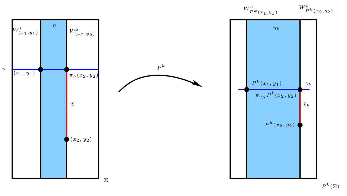
Figure 5. Action of $P^{k}$.

Hence, $P^{k}|_{\eta}$ is a diffeomorphism between the strips $\eta$ and $\eta_{k}$ that maps the interval ${\mathcal{I}}$, bounded by $(x_{2},y_{2})$ and $\pi_{\gamma}(x_{2},y_{2})$ inside $W^{s}_{(x_{2},y_{2})}$, to the interval ${\mathcal{I}}_{k}$ bounded by $P^{k}(x_{2},y_{2})$ and $\pi_{\gamma_{k}}P^{k}(x_{2},y_{2})$ inside $W^{s}_{P^{k}(x_{2},y_{2})}$. Thus,

$$|X_{u}(x_{1},y_{1})-X_{u}(x_{2},y_{2})| \leq|X_{u}(x_{1},y_{1})-P^{k}(x_{1},y_{1})|+|P^{k}(x_{1},y_{1})-P^{k}(x_{2},y_{2})|$$

$$\qquad+|P^{k}(x_{2},y_{2})-X_{u}(x_{2},y_{2})|.$$

We also have by uniform contractions of the stable foliation a constant $C>0$ so that

$$|P^{k}(x_{1},y_{2})-P^{k}(x_{2},y_{2})| \leq\operatorname{diam}(\gamma_{k}\cap\eta_{k})+\operatorname{diam}({\mathcal{I}}_{k})$$

$$\leq C|f^{k}_{\gamma_{k}}\pi_{\gamma_{k}}(x_{1},y_{1})-f^{k}_{\gamma_{k}}\pi_{\gamma_{k}}(x_{2},y_{2})|+\sigma^{k}\operatorname{diam}({\mathcal{I}})$$

$$\leq C|f^{k}\pi_{\gamma}(x_{1},y_{1})-f^{k}\pi_{\gamma}(x_{2},y_{2})|+\sigma^{k}\operatorname{diam}({\mathcal{I}})$$

$$\leq C\sigma^{R(x_{1})-k}|F(x_{1})-F(x_{2})|+\sigma^{k}|y_{1}-y_{2}|,$$ (5.2)

where we have used (3.1) (to compare $f_{\gamma_{k}}$ with $f$) and (4.4).

We also have that $|X_{u}(x_{1},y_{1})-P^{k}(x_{1},y_{1})|+|X_{u}(x_{2},y_{2})-P^{k}(x_{2},y_{2})|$ equals

$$|X_{u}(x_{1},y_{1}) -X_{\tau_{k}(x_{1})}(x_{1},y_{1})|+|X_{u}(x_{2},y_{2})-X_{\tau_{k}(x_{2})}(x_{2},y_{2})|$$

$$\leq|X|_{\infty}(u-\tau_{k}(x_{1}))+|X|_{\infty}(\tau_{k}(x_{2})-u)$$

$$\leq C|X|_{\infty}|F(x_{1})-F(x_{2})|^{\alpha},$$

where in the last inequality we used Lemma 5.10.

Thus, it follows that there exists a constant $C>0$ such that

$$|X_{u}(x_{1},y_{1})-X_{u}(x_{2},y_{2})|\leq C(|F(x_{1})-F(x_{2})|^{\alpha}+|y_{1}-y_{2}|).$$

Now consider $\ell=k$. In this case, let $\xi=u-\tau_{k-1}(x_{1})$ and $\xi^{\prime}=u-\tau_{k-1}(x_{2})$ and

$$|X_{u}(x_{1},y_{1})-X_{u}(x_{2},y_{2})| \leq|X_{u}(x_{1},y_{1})-X_{\xi}(P^{k-1}(x_{2},y_{2}))|$$ (5.3)

$$\qquad+|X_{\xi}(P^{k-1}(x_{2},y_{2}))-X_{u}(x_{2},y_{2})|.$$

We also have by Lemma 5.10 that

$$|X_{\xi}(P^{k-1}(x_{2},y_{2}))-X_{u}(x_{2},y_{2})| =|X_{\xi}(P^{k-1}(x_{2},y_{2}))-X_{\xi^{\prime}}(P^{k-1}(x_{2},y_{2}))|$$

$$\leq|X|_{\infty}|\xi-\xi^{\prime}|=|X|_{\infty}|\tau_{k-1}(x_{1})-\tau_{k-1}(x_{2})|$$ (5.4)

$$\leq C|F(x_{1})-F(x_{2})|^{\alpha}.$$

If $P^{k-1}(x_{i},y_{i})$, $i=1,2$, are in a ingoing cross-section for a tubular neighborhood, then there exists a constant $C>0$ so that $|X_{u}(x_{1},y_{2})-X_{\xi}(P^{k-1}(x_{2},y_{2}))|$ equals

$$|X_{\xi}(P^{k-1}(x_{1},y_{1}))-X_{\xi}(P^{k-1}(x_{2},y_{2}))|\leq C|P^{k-1}(x_{1},y_{1})-P^{k-1}(x_{2},y_{2})|$$

Analogously to the case $\ell=k+1$ (see inequality (5.2)) we have that $|P^{k-1}(x_{1},y_{2})-P^{k-1}(x_{2},y_{2})|\leq C|F(x_{1})-F(x_{2})|+|y_{1}-y_{2}|$ and the result follows.

Now suppose that $P^{k-1}(x_{i},y_{i})$, $i=1,2$, are in a ingoing cross-section for a flow-box around a singularity. Without loss of generality we also assume that $\tau(f^{k-1}(x_{1}))\leq\tau(f^{k-1}(x_{2}))$. Note that $\xi=u-\tau_{k-1}(x_{1})\leq\tau(f^{k-1}(x_{1}))$. Let $\eta_{k-1}$ be the strip determined by $W^{s}_{P^{k-1}(x_{1},y_{1})}$ and $W^{s}_{P^{k-1}(x_{2},y_{2})}$ (see Figure 6). Again, there is no singular leaf in $\eta_{k-1}$, otherwise $P^{k-1}(x_{1},y_{1})$ and $P^{k-1}(x_{2},y_{2})$ wouldn’t be in the same element of $\widehat{\mathcal{P}}$. Hence $P^{k-1}(x_{1},y_{1})$ and $P^{k-1}(x_{2},y_{2})$ will hit the same cross-section in the future.

Let $\Sigma_{k-1},\Sigma_{k}\in\Xi$ be such that $P^{j}(x_{i},y_{i})\in\Sigma_{j}$, for $i\in\{1,2\}$ and $j\in\{k-1,k\}$. We also define $\eta_{k}=P(\eta_{k-1})\subset\Sigma_{k}$ and $\widehat{\eta}_{k}=X_{\tau(x_{1})}(\eta_{k-1})$ (see Figure 6).

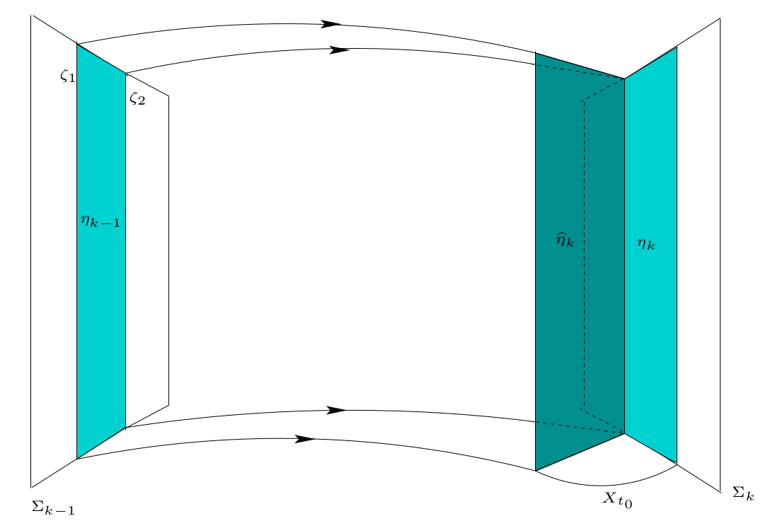
Figure 6. Case $\ell=k$ and traveling in a flow-box.

Because the orbits are in a neighborhood of a Lorenz-like singularity we claim that $|\tau(f^{k-1}(x_{1}))-\tau(f^{k-1}(x_{2}))|$ is bounded. Indeed, from Lemma 3.13 there is a constant $C>0$ so that this expression is bounded from above by

$$C \dfrac{|f^{k-1}(x_{1})-f^{k-1}(x_{2})|}{\min\{\operatorname{dist}(f^{k-1}(x_{1}),{\mathcal{D}}),\operatorname{dist}(f^{k-1}(x_{2}),{\mathcal{D}})\}}+|f^{k-1}(x_{1})-f^{k-1}(x_{2})|^{\alpha}$$

$$\leq C\left(\dfrac{\sigma^{R(x_{1})-k+1}}{\sigma^{b(R(x_{1})-k+1)}}+\sigma^{\alpha(R(x_{1})-k+1)}\right)|F(x_{1})-F(x_{2})|^{\alpha}.$$

Since $0<b<1/2$, it follows that the right hand side of the inequality above is bounded by a constant as we claimed. Because $\tau(f^{k-1}(x_{1}))\leq\tau(f^{k-1}(x_{2}))$, we have that $X_{\tau(f^{k-1}(x_{1}))}(\zeta_{1})\in\Sigma_{k}$ while $X_{\tau(f^{k-1}(x_{1}))}(\zeta_{2})$ is yet about to hit $\Sigma_{k}$; see Figure 6. Because $t_{0}:=|\tau(f^{k-1}(x_{1}))-\tau(f^{k-1}(x_{2}))|$ is bounded we have that $\widehat{\eta}_{k}$ is diffeomorphic to $\eta_{k-1}$ by a diffeomorphism that distorts distances at most by a constant factor. In particular, letting $\zeta_{i}=W^{s}_{f^{k-1}(x_{i})}$, $i=1,2$, there exists a constant $C>0$ such that $\operatorname{dist}(X_{\tau(\zeta_{1})}(\zeta_{1}),X_{\tau(\zeta_{1})}(\zeta_{2}))\leq C\operatorname{dist}(X_{\tau(\zeta_{1})}(\zeta_{1}),X_{\tau(\zeta_{2})}(\zeta_{2})).$

If we restrict the flow to a central-unstable invariant manifold $W=W_{\sigma}$ in a neighborhood of $\sigma$, as in the proof of Lemma 3.13 using a smooth linearization, then the points $\xi_{1}=W\cap\zeta_{1}$ and $\xi_{2}=W\cap\zeta_{2}$ move away from each other at a uniform rate, that is $\operatorname{dist}(X_{t}(\xi_{1}),X_{t}(\xi_{2}))\leq Ce^{-\lambda(\tau(\zeta_{1})-t)}\operatorname{dist}(X_{\tau(\zeta_{1})}(\xi_{1}),X_{\tau(\zeta_{2})}(\xi_{2}))$, for all $0<t<\tau(\zeta_{1})$, where $\lambda>0$ is the expanding eigenvalue at the singularity. Since the stable foliation is of class $C^{2}$ and transverse to $W$, we can write $V_{\sigma}$ as a product $V_{\sigma}=W_{\sigma}\times D$ where $D$ is a $d_{s}$-dimensional disk and the identification is given by a $C^{1+}$ diffeomorphism (the smoothness provided by Lemma 3.12). Hence we can extend the previous estimate for $\xi_{1},\xi_{2}$ to the entire local stable leaf in $V_{\sigma}$ by at most a constant factor, that is $\operatorname{dist}(X_{t}(\zeta_{1}),X_{t}(\zeta_{2}))\leq Ce^{-\lambda(\tau(\zeta_{1})-t)}\operatorname{dist}(X_{\tau(\zeta_{1})}(\zeta_{1}),X_{\tau(\zeta_{2})}(\zeta_{2}))$ for $0<t<\tau(x_{1})$. In particular, we arrive at $|X_{\xi}(P^{k-1}(x_{1},y_{1}))-X_{\xi}(P^{k-1}(x_{2},y_{2}))|\leq C|P^{k}(x_{1},y_{1})-P^{k}(x_{2},y_{2})|.$

Finally $|X_{u}(x_{1},y_{2})-X_{\xi}(P^{k-1}(x_{2},y_{2}))|\leq|F(x_{1})-F(x_{2})|+|y_{1}-y_{2}|$ by inequality (5.2) and the result follows.

To conclude the proof we consider the case $x_{1},x_{2}\in Q$ with $|F(x_{1})-F(x_{2})|\geq\varepsilon$. Since $M$ is a compact we can set $K:=\sup_{(t,z)\in{\mathbb{R}}\times M}|X_{u}(z)|<\infty$. Hence,

$$|X_{u}(x_{1},y_{1})-X_{u}(x_{2},y_{2})| \leq 2K\leq\dfrac{2K}{\varepsilon}|F(x_{1})-F(x_{2})|$$

$$\leq C(|F(x_{1})-F(x_{2})|^{\alpha}+|y_{1}-y_{2}|),$$

letting $C>0$ bigger so that $C>2k/\varepsilon$ if necessary. ∎

We are finally ready to present

Proof of Theorem 5.8.

By the Mean Value Theorem, there is a $u\in(u_{1},u_{2})$ such that

$$|p(x_{2},y_{2},u_{1})-p(x_{2},y_{2},u_{2})|=|X_{u_{1}}(x_{2},y_{2})-X_{u_{2}}(x_{2},y_{2})|\leq|X|_{\infty}|u_{1}-u_{2}|.$$

Now $|p(x_{1},y_{1},u_{1})-p(x_{2},y_{2},u_{2})|$ is bounded above by

$$|p(x_{1},y_{1},u_{1})-p(x_{2},y_{2},u_{1})| +|p(x_{2},y_{2},u_{1})-p(x_{2},y_{2},u_{2})|$$

$$\leq|X_{u_{1}}(x_{1},y_{1})-X_{u_{1}}(x_{2},y_{2})|+|X|_{\infty}|u_{1}-u_{2}|$$

$$\leq C(|F(x_{1})-F(x_{2})|^{\alpha}+|y_{1}-y_{2}|+|u_{1}-u_{2}|),$$

for some constant $C>0$, as desired, after using Proposition 5.11. ∎

5.3. Exponential mixing

We deduce here Theorem A from Theorem 2.5.

Proof of Theorem A.

It follows from Theorem 2.5 that if $\varphi\in C^{1}(U)$ and $\psi\in C^{3}(U)$, then $\varphi\circ p\in C^{\alpha}_{\text{loc}}(\widehat{\Delta}^{r})$ and $\psi\circ p\in C^{\alpha,2}_{\text{loc}}(\widehat{\Delta}^{r})$ for each skew product semiflow associated to each ergodic physical measure supported in $U$.

Hence, using item 3 of Theorem 1.8 we get $s_{i}\geq 0$, $\sum_{i=1}^{k}s_{i}=1$ and $\mu=\sum_{i}s_{i}\mu_{i}$ where each $\mu_{i}$ is an ergodic physical measure for $X$ supported in the attracting set $\Lambda$. Theorem 2.5 ensures that $\mu=\sum_{i}s_{i}\cdot(p_{i})_{*}\big{(}\mu_{\hat{F}_{i}}^{r_{i}}\big{)}$. We normalize the observable $\varphi$ by defining $\bar{\varphi}=\sum_{i=1}^{k}s_{i}(\varphi-\mu_{i}(\varphi))\chi_{B(\mu_{i})}$ which satisfies $\mu_{i}(\bar{\varphi})=0$ and also $\bar{\varphi}\circ p_{i}=s_{i}\big{(}\varphi\circ p_{i}-\mu_{i}(\varphi))\in C^{\alpha}_{loc}(\widehat{\Delta}_{i}^{r_{i}})$ for all $i=1,\dots,k$.

Combining this with Theorem 2.4 we conclude that

$$\Big{|}\int(\varphi\circ X_{t})\psi\,d\mu -\int\varphi\,d\mu\int\psi\,d\mu\Big{|}=\left|\int\big{(}\varphi\circ X_{t}-\mu(\varphi))\psi\,d\mu\right|$$

$$=\left|\int\bar{\varphi}\circ X_{t}\cdot\psi\,d\mu\right|\leq\sum_{i}s_{i}\left|\int(\bar{\varphi}\circ p_{i}\circ\widehat{F_{i}}^{t})\cdot\psi\circ p_{i}\,d\mu^{r_{i}}_{\widehat{F}_{i}}\right|$$

$$\leq\sum_{i}s_{i}C_{i}e^{-c_{i}t}\|\bar{\varphi}\circ p_{i}\|_{\alpha}\|\psi\circ p_{i}\|_{\alpha,2}$$

$$\leq Ce^{-ct}\sum_{i}s_{i}\|\varphi\circ p_{i}\|_{\alpha}\|\psi\circ p_{i}\|_{\alpha,2}$$

for some $C,c>0$, since the number $k$ of ergodic physical measures is finite and $\varphi$ is bounded. Using Theorem 2.5 again we get

$$\left|\int(\varphi\circ X_{t})\cdot\psi\,d\mu-\int\varphi\,d\mu\int\psi\,d\mu\right|\leq C^{3}e^{-ct}|\varphi|_{C^{1}}|\psi|_{C^{3}}.$$

Finally, let us fix $\eta\in(0,1)$ and $\varphi,\psi\in C^{\eta}(U)$. Given $\delta>0$ we can choose $\tilde{\varphi},\tilde{\psi}\in C^{3}(U)$ such that $|\varphi-\tilde{\varphi}|_{\infty}<\delta^{\eta}\|\varphi\|_{\eta}$ and $|\tilde{\varphi}|_{C^{1}}\leq\delta^{-1}\|\varphi\|_{\eta}$; and also $|\psi-\tilde{\psi}|_{\infty}<\delta^{\eta}\|\psi\|_{\eta}$ with $|\tilde{\psi}|_{C^{3}}\leq\delta^{-3}\|\psi\|_{\eta}$.

Then, if we denote $\rho(\varphi,\psi,t)=\mu(\psi\cdot\varphi\circ X_{t})-\mu(\varphi)\mu(\psi)$ and the constants of the last estimate as $\tilde{C},\tilde{c}>0$, we get

$$|\rho(\varphi,\psi,t) -\rho(\tilde{\varphi},\tilde{\psi},t)|\leq 2|\varphi-\tilde{\varphi}|_{\infty}|\psi|_{\infty}+2|\tilde{\varphi}|_{\infty}|\psi-\tilde{\psi}|_{\infty}$$

$$\leq 2\|\varphi\|_{\eta}\delta^{\eta}\|\psi\|_{\eta}+2|\tilde{\varphi}|_{\infty}\|\psi\|_{\eta}\delta^{\eta}\leq 2\|\varphi\|_{\eta}\|\psi\|_{\eta}\delta^{\eta}+4\|\varphi\|_{\eta}\|\psi\|_{\eta}\delta^{\eta}$$

since $|\tilde{\varphi}|_{\infty}\leq|\varphi|_{\infty}+|\varphi-\tilde{\varphi}|_{\infty}\leq\|\varphi\|_{\eta}(1+\delta^{\eta})\leq 2\|\varphi\|_{\eta}$. Moreover, we also have $|\rho(\tilde{\varphi},\tilde{\psi},t)|\leq\tilde{C}e^{-\tilde{c}t}|\tilde{\varphi}|_{C^{3}}|\tilde{\psi}|_{C^{3}}\leq\tilde{C}e^{-\tilde{c}t}\delta^{-4}\|\varphi\|_{\eta}\|\psi\|_{\eta}$, thus

$$|\rho(\varphi,\psi,t)| \leq\|\varphi\|_{\eta}\|\psi\|_{\eta}(\tilde{C}\delta^{-4}e^{-\tilde{c}t}+6\delta^{\eta}).$$

Setting $\delta=e^{-\tilde{c}t/(4+\eta)}$ we obtain a constant $C>0$ so that

$$|\rho(\varphi,\psi,t)| \leq Ce^{-\eta\tilde{c}t/(4+\eta)}\|\varphi\|_{\eta}\|\psi\|_{\eta},\quad t>0.$$

This completes the proof after setting the exponent $c=\eta\tilde{c}/(4+\eta)$. ∎

5.4. Exponential convergence to equilibrium

To prove exponential convergence to equilibrium for the flow, that is, Corollary B, we need the following corollary of Theorem 2.4 whose proof we postpone to Subsection 6.2.2. We denote the Lebesgue measure in $\widehat{\Delta}^{r}$ by $\operatorname{Leb}^{r}_{3}$, that is, $\operatorname{Leb}^{r_{i}}_{3}:=(\operatorname{Leb}_{\widehat{\Delta_{i}}}\times\operatorname{Leb}_{\mathbb{R}})/\int r_{i}\,d\operatorname{Leb}_{\widehat{\Delta}}$ corresponding to each one of the ergodic physical measures $\mu_{i}$ supported on the attracting set.

Corollary 5.12 (Exponential convergence to equilibrium for $\widehat{F}_{t}$).

In the same setting of Theorem 2.4 there exist constants $c,C>0$ such that

$$\left|\int(\varphi\circ\widehat{F}_{t})\psi\,d\operatorname{Leb}^{r}_{3}-\int\varphi d\mu^{r}_{\widehat{F}}\int\psi\,d\operatorname{Leb}^{r}_{3}\right|\leq Ce^{-ct}\|\varphi\|_{\alpha}\|\psi\|_{\alpha,2},$$

for all $\varphi\in C^{\alpha}_{\text{loc}}(\widehat{\Delta}^{r})$, $\psi\in C^{\alpha,2}_{\text{loc}}(\widehat{\Delta}^{r})$ and $t>0$.

Now we use this to complete the proof of the remaining main result.

Proof of Corollary B.

We argue similarly to the proof of Theorem A using the decomposition $\operatorname{Leb}=\sum_{i}\vartheta_{i}\operatorname{Leb}_{i}$ and $\widetilde{\mu}=\sum_{i}\vartheta_{i}\mu_{i}$ to write for $\varphi,\psi\in C^{1}(U)$

$$\Big{|}\int(\varphi\circ X_{t})\psi\,d\operatorname{Leb} -\int\varphi\,d\mu\int\psi\,d\operatorname{Leb}\Big{|}=\left|\int\big{(}\varphi\circ X_{t}-\mu(\varphi))\psi\,d\operatorname{Leb}\right|$$

$$=\left|\int\bar{\varphi}\circ X_{t}\cdot\psi\,d\operatorname{Leb}\right|\leq\sum_{i}\vartheta_{i}\left|\int\bar{\varphi}\circ X_{t}\cdot\psi\,d\operatorname{Leb}_{i}\right|$$

where $\bar{\varphi}$ is just as in the proof of Theorem A. Now we have $\operatorname{Leb}_{i}=\xi_{i}\cdot(p_{i})_{*}\operatorname{Leb}_{3}^{r_{i}}$ where $\xi_{i}$ is the Jacobian of $p_{i}(w,u)=X_{u}(w)$, which depends on the Jacobian of the flow of $X$, which is of class $C^{1}$ since the vector field $X$ is of class $C^{2}$.

Moreover, $\xi_{i}$ is strictly positive and uniformly bounded since, by strong dissipativeness, we have that the divergence of the vector field is strictly negative in a neighborhood of $\Lambda$: there exists $\vartheta>0$ so that $\operatorname{div}X<-\vartheta<0$ on $U$. Hence

$$\xi_{i}(w,u)=|\det Dp_{i}(w,u)| \leq\frac{\|X(X_{u}w)\|}{\|X(w)\|}\cdot|\det DX_{u}(w)|$$

$$=\frac{\|X(X_{u}w)\|}{\|X(w)\|}\cdot\exp\int_{0}^{u}(\operatorname{div}X)(X_{s}(w))\,ds\leq Ce^{-\vartheta u}$$

where the constant $C>0$ depends only on the lenght of the vector field in a neighborhood of $\Lambda$. Thus $\xi_{i}\in C^{1}(U)$. We can therefore write

$$\sum_{i}\vartheta_{i} \left|\int\bar{\varphi}\circ X_{t}\cdot\psi\,d\operatorname{Leb}_{i}\right|=\sum_{i}\vartheta_{i}\left|\int\bar{\varphi}\circ X_{t}\cdot(\psi\xi_{i})\,d(p_{i})_{*}\operatorname{Leb}_{3}^{r_{i}}\right|.$$

At this point, we approximate $\psi\xi_{i}$ by a $C^{3}$ function: for a given $0<\delta<1$ we choose $\tilde{\psi}\in C^{3}(U)$ so that $|\psi\xi_{i}-\tilde{\psi}|_{\infty}\leq\delta|\psi\xi_{i}|_{C^{1}}$ and $|\tilde{\psi}|_{C^{3}}\leq\delta^{-3}|\psi\xi_{i}|_{C^{1}}.$ On the one hand

$$\left|\int\!\!\tilde{\psi}\cdot\bar{\varphi}\circ X_{t}\,d(p_{i})_{*}\!\operatorname{Leb}_{3}^{r_{i}}\!\!-\!\!\int\!\!(\psi\xi_{i})\cdot\bar{\varphi}\circ X_{t}\,d(p_{i})_{*}\!\operatorname{Leb}_{3}^{r_{i}}\right|\leq|\bar{\varphi}|_{\infty}|\tilde{\psi}-\psi\xi_{i}|_{\infty}\leq\delta|\bar{\varphi}|_{C^{1}}|\psi\xi_{i}|_{C^{1}}$$

while on the other hand, by Corollary 5.12 and Theorem 2.5

$$\left|\int\bar{\varphi}\circ X_{t}\cdot\tilde{\psi}\,d(p_{i})_{*}\operatorname{Leb}_{3}^{r_{i}}\right| =\left|\int(\bar{\varphi}\circ p_{i}\circ\widehat{F_{i}}^{t})\cdot\tilde{\psi}\circ p_{i}\,d\operatorname{Leb}_{3}^{r_{i}}\right|$$

$$\leq C_{i}e^{-c_{i}t}\|\bar{\varphi}\circ p_{i}\|_{\alpha}\|\tilde{\psi}\circ p_{i}\|_{\alpha,2}$$

$$\leq C^{2}C_{i}e^{-c_{i}t}|\varphi|_{C^{1}}|\tilde{\psi}|_{C^{3}}\leq C^{2}C_{i}e^{-c_{i}t}\delta^{-3}|\varphi|_{C^{1}}|\psi\xi_{i}|_{C^{1}}.$$

So we obtain

$$\left|\int\bar{\varphi}\circ X_{t}\cdot(\psi\xi_{i})\,d(p_{i})_{*}\operatorname{Leb}_{3}^{r_{i}}\right| \leq C^{2}C_{i}e^{-c_{i}t}\delta^{-3}|\varphi|_{C^{1}}|\psi\xi_{i}|_{C^{1}}+\delta|\bar{\varphi}|_{C^{1}}|\psi\xi_{i}|_{C^{1}}$$

$$\leq\tilde{C}_{i}e^{-c_{i}t/4}|\varphi|_{C^{1}}|\psi|_{C^{1}}$$

for some constant $\tilde{C}_{i}>0$, after setting $\delta=e^{-c_{i}t/4}$. Since this holds for each $i$, we get

$$\Big{|}\int(\varphi\circ X_{t})\psi\,d\operatorname{Leb} -\int\varphi\,d\mu\int\psi\,d\operatorname{Leb}\Big{|}\leq\sum_{i}s_{i}\left|\int\bar{\varphi}\circ X_{t}\cdot(\psi\xi_{i})\,d(p_{i})_{*}\operatorname{Leb}_{3}^{r_{i}}\right|.$$

$$\leq\sum_{i}s_{i}C_{i}e^{-c_{i}t/4}|\varphi|_{C^{1}}|\psi|_{C^{1}}\leq Ce^{-ct}|\varphi|_{C^{1}}|\psi|_{C^{1}}$$

for some constants $C,c>0$ by finiteness of the number $k$ of physical measures.

Having established the result for smooth observables $\varphi,\psi\in C^{1}(U)$, we can now extend it to Hölder observables $\varphi,\psi\in C^{\eta}(U)$ for any $0<\eta<1$ using the exact same arguments as in the proof of Theorem A. ∎

6. Exponential mixing and convergence to equilibrium for hyperbolic skew product semiflows

In this chapter we present the proof of Theorems 2.2 and 2.4. Because the proof of these theorems follow the same steps as of [10] we only prove the parts that differ and refer to parts that are equal.

From now on use the following convention: given two real sequences $(a_{n})_{n}$ and $(b_{n})_{n}$, we write $a_{n}\lesssim b_{n}$ if there is a constant $C>0$ such that $a_{n}\leq Cb_{n}$, for all $n\geq 1$.

6.1. Exponential mixing for $C^{1+\alpha}$ expanding semiflows

In this section we prove Theorem 2.2. This theorem is a generalization of [10, Theorem 2.1] to the function space $C^{\alpha,2}_{\text{loc}}(\Delta^{r})$ (recall the definition of this space on Subsection 2.1.3). In the proof we use the results of [10] as much as possible and show the adaptations in the places where they are required.

Throughout this section we consider $F:\Delta\to\Delta$ to be a $C^{1+\alpha}$ uniformly expanding map and $r:\Delta\to(0,+\infty)$ a function satisfying conditions (iii) - (v) (recall Subsection 2.1.1). Setting $r_{n}=\sum^{n-1}_{j=0}r\circ F^{j}$, we note that we can generalize the items (ii) and (iii) of Subsection 2.1.1 as: there exists a constant $C>0$ such that ($\text{ii}_{1}$) $|\log|h^{\prime}||_{\alpha}\leq C$; and $(iii)_{1}$ $|(r_{n}\circ h)^{\prime}|_{\infty}\leq C$ for all $h\in\mathcal{H}_{n}$ and all integer $n\geq 1$

We need to use an equivalent form of the UNI condition (see [22, Proposition 7.4]):

UNI - equivalent formulation:

there exist $D>0$, $n_{0}\geq 1$ sufficiently large and $h_{1},h_{2}\in\mathcal{H}_{n_{0}}$ so that $\inf|(r_{n}\circ h_{1}-r_{n}\circ h_{2})^{\prime}|\geq D.$

6.1.1. Twisted transfer operator

Here we work with complex observables so we denote by $C^{\alpha}(\Delta)$ the space of functions $\psi:\Delta\to{\mathbb{C}}$ such that $\|\psi\|_{\alpha}=|\psi|_{\infty}+|\psi|_{\alpha}<\infty$ and $C^{\alpha}_{\text{loc}}(\Delta)$ the space of functions $\psi:\Delta\to{\mathbb{C}}$ such that $\|\psi\|_{\alpha}=|\psi|_{\infty}+|\psi|_{\alpha,\text{loc}}<\infty$, where

$$|\psi|_{\alpha,\text{loc}}=\sup_{h\in\mathcal{H}}\sup_{x\neq y}\dfrac{|\psi(hx)-\psi(hy)|}{|x-y|^{\alpha}}.$$

It is also convenient to introduce the family of equivalent norms: for all $b\in{\mathbb{R}}$

$$\|\psi\|_{b}=\max\{|\psi|_{\infty},|\psi|_{\alpha,\text{loc}}/(1+|b|^{\alpha})\},\quad\psi\in C^{\alpha}_{\text{loc}}(\Delta).$$

For each $s\in{\mathbb{C}}$ we denote by $P_{s}$ the non-normalized twisted transfer operator, that is,

$$P_{s}=\sum_{h\in\mathcal{H}}A_{s,h}\quad\text{where}\quad A_{s,h}\psi=e^{-sr\circ h}|h^{\prime}|\psi\circ h.$$

In what follows we present the result that guarantees that $P_{s}$ is well defined.

Proposition 6.1.

[10, Proposition 2.5] Write $s=\sigma+ib$. There exists $\varepsilon\in(0,1)$ such that the family $s\mapsto P_{s}$ of operators on $C^{\alpha}(\Delta)$ is continuous on $\{\sigma>-\varepsilon\}$. Moreover, $\sup_{|\sigma|<\varepsilon}\|P_{s}\|_{b}<\infty$.

Remark 6.2.

Using that $|\psi(hx)-\psi(hy)|\leq|\psi|_{\alpha,\text{loc}}|x-y|^{\alpha}$ in the proof of Proposition 6.1 we note that we can define $P_{s}$ on $C^{\alpha}_{\text{loc}}(\Delta)$ and its range remain in $C^{\alpha}(\Delta)$ when $\Re s>-\varepsilon$. Moreover, it also follows from the proof that $\|P_{s}\psi\|_{b}\leq\widetilde{C}\|\psi\|_{b}$, where $\widetilde{C}:=C(1+|\sigma|+|b|^{\alpha})(1+|b|^{\alpha})^{-1}\sum_{h\in\mathcal{H}}e^{\varepsilon|r\circ h|_{\infty}}|h^{\prime}|_{\infty}$.

The unperturbed operator $P_{0}$ has a simple leading eigenvalue $\lambda_{0}=1$ with strictly positive $C^{\alpha}$ eigenfunction $f_{0}$. By Proposition 6.1, there exists $\varepsilon\in(0,1)$ such that $P_{\sigma}$ has a continuous family of simple eigenvalues $\lambda_{\sigma}$ for $|\sigma|<\varepsilon$ with associated $C^{\alpha}$ eigenfunctions $f_{\sigma}$. Shrinking $\varepsilon$ if necessary, we can ensure that $\lambda_{\sigma}>0$ and $f_{\sigma}$ is strictly positive for $|\sigma|<\varepsilon$.

Remark 6.3.

By standard perturbation theory, for any $\delta>0$ there exists $\varepsilon\in(0,1)$ such that $\sup_{|\sigma|<\varepsilon}|\lambda_{\sigma}-1|<\delta$, $\sup_{|\sigma|<\varepsilon}|f_{\sigma}/f_{0}-1|_{\infty}<\delta$ and $\sup_{|\sigma|<\varepsilon}|f_{\sigma}/f_{0}-1|_{\alpha}<\delta$. In particular, we may assume that $1/2\leq\lambda_{\sigma}\leq 2$, $f_{0}/2\leq f_{\sigma}\leq 2f_{0}$ and $|f_{0}|_{\alpha}/2\leq|f_{\sigma}|\alpha\leq 2|f_{0}|_{\alpha}$.

For $s=\sigma+ib$ with $|\sigma|<\varepsilon$, we define the normalized transfer operators

$$\mathcal{L}_{s}\psi=(\lambda_{\sigma}f_{\sigma})^{-1}P_{s}(f_{\sigma}\psi)=(\lambda_{\sigma}f_{\sigma})^{-1}\sum_{h\in\mathcal{H}}A_{s,h}(f_{\sigma}\psi).$$

It also follows that $\mathcal{L}_{s}$ is defined on $C^{\alpha}_{\text{loc}}(\Delta)$ with range on $C^{\alpha}(\Delta)$ for all $s$ where $P_{s}$ is defined. Note that $\mathcal{L}_{\sigma}1=1$ for all $\sigma$ and $|\mathcal{L}_{s}|_{\infty}\leq 1$ for all $s$ (where defined).

Using Remark 6.2, the strategy that we follow now is to take the results of [10] that depend on observables $\psi\in C^{\alpha}(\Delta)$, change them to $P_{s}\psi$ or ${\mathcal{L}}_{s}\psi$, with $\psi\in C^{\alpha}_{\text{loc}}(\Delta),$ and explain why these changes are enough to prove Theorem 2.2.

6.1.2. Lasota-Yorke inequality

Note that

$$\mathcal{L}^{n}_{s}\psi=\lambda^{-n}_{\sigma}f^{-1}_{\sigma}\sum_{h\in\mathcal{H}_{n}}A_{s,h,n}(f_{\sigma}\psi),\text{ where }A_{s,h,n}\psi:=e^{-sr_{n}\circ h}|h^{\prime}|\psi\circ h.$$

Lemma 6.4.

[10, Lemma 2.7] There is a constant $C>1$ such that

$$|{\mathcal{L}}^{n}_{s}\psi|_{\alpha}\leq C(1+|b|^{\alpha})|\psi|_{\infty}+C\rho^{n}|\psi|_{\alpha}\leq C(1+|b|^{\alpha})\{|\psi|_{\infty}+\rho^{n}\|\psi\|_{b}\},$$

for all $s=\sigma+ib$, $|\sigma|<\varepsilon$, $n\geq 1$ and all $\psi\in C^{\alpha}(\Delta)$.

Lemma 6.5.

[10, Lemma 2.7 adapted] There is a constant $C>1$ such that

$$|\mathcal{L}^{n+1}_{s}\psi|_{\alpha}\leq C(1+|b|^{\alpha})|\psi|_{\infty}+C\rho^{n}|\psi|_{\alpha,\text{loc}}\leq C(1+|b|^{\alpha})\{|\psi|_{\infty}+\rho^{n}\|\psi\|_{b}\},$$

for all $s=\sigma+ib$, $|\sigma|<\varepsilon$, $n\geq 1$ and all $\psi\in C^{\alpha}_{\text{loc}}(\Delta)$.

Proof.

As ${\mathcal{L}}_{s}\psi\in C^{\alpha}(\Delta)$ for all $\psi\in C^{\alpha}_{\text{loc}}(\Delta)$, using the original result [10, Lemma 2.7] we get that there exists $C>1$ so that $|{\mathcal{L}}^{n+1}_{s}\psi|_{\alpha}\leq C(1+|b|^{\alpha})|{\mathcal{L}}_{s}\psi|_{\infty}+C\rho^{n}|{\mathcal{L}}_{s}\psi|_{\alpha}.$ Using Remarks 6.2 and 6.3 we get that $|{\mathcal{L}}_{s}\psi|_{\alpha}\lesssim|\psi|_{\alpha,\text{loc}}$ for all $\psi\in C^{\alpha}_{\text{loc}}(\Delta)$. The results follows since we also have that $|{\mathcal{L}}_{s}|_{\infty}\leq 1$. ∎

Corollary 6.6.

There exists $C>1$ such that $\|{\mathcal{L}}_{s}^{n}\|_{b}\leq C$ for all $s=\sigma+ib$, with $|\sigma|<\varepsilon$ and all $n\geq 1$.

Proof.

It is clear that $|{\mathcal{L}}^{n}_{s}\psi|_{\infty}\leq|\psi|_{\infty}\leq\|\psi\|_{b}$, for all $n\geq 1$. By Lemma 6.5, there exists $C>1$ such that $|{\mathcal{L}}^{n}_{s}\psi|_{\alpha}\leq C(1+|b|^{\alpha})\|\psi\|_{b}$, for all $n\geq 2$, for all $\psi\in C^{\alpha}_{\text{loc}}(\Delta)$. For $n=1$ we have by Remark 6.2 that there exists $\widetilde{C}>1$ such that $|{\mathcal{L}}_{s}\psi|_{\alpha}\leq\widetilde{C}|\psi|_{\alpha,\text{loc}}\leq\widetilde{C}\|\psi\|_{b}$, for all $\psi\in C^{\alpha}_{\text{loc}}(\Delta)$. Hence, taking a bigger $C$ the result follows. ∎

In the following lemma the constant $C_{0}$ is the constant $C_{4}$ from the definition of the family of cones ${\mathcal{C}}_{b}$ in [10, Subsection 2.3]. For our needs it is not necessary to enter in the details of cone invariance because we only need to adapt the existing results of [10].

Lemma 6.7.

[10, Corollary 2.15 adapted] There exist $\varepsilon,\beta\in(0,1)$ and $A,C>0$ such that $\|{\mathcal{L}}^{4mn_{0}+1}_{s}\psi\|_{b}\leq C\beta^{m}\|\psi\|_{b}$ for all $m\geq A\log|b|$, $s=\sigma+ib$, $|\sigma|<\varepsilon$, $|b|\geq\max\{4\pi/D,1\}$ and all $\psi\in C^{\alpha}_{\text{loc}}(\Delta)$ satisfying $|{\mathcal{L}}_{s}\psi|_{\alpha}\leq C_{0}|b|^{\alpha}|{\mathcal{L}}_{s}\psi|_{\infty}$.

Proof.

The result follows directly from [10, Corollary 2.15] using ${\mathcal{L}}_{s}\psi$ in the place of $\psi$ for $\psi\in C^{\alpha}_{\text{loc}}(\Delta)$. ∎

For the next theorem, if $C$ is the constant given by Lemma 6.4 and $\widetilde{C}>0$ is such that $\|{\mathcal{L}}_{s}\psi\|_{b}\leq\widetilde{C}\|\psi\|_{b}$, for all $\psi\in C^{\alpha}_{\text{loc}}(\Delta)$, we require that $\max\{2C\widetilde{C}C^{-1}_{0},2\widetilde{C}C^{-1}_{0}\}<1/3$. We also fix $n_{0}$ from UNI condition such that $C\widetilde{C}\rho^{n_{0}-1}<1/3$.

Theorem 6.8.

Let $D^{\prime}=\max\{4\pi/D,2\}$. There exist $\varepsilon,\gamma\in(0,1)$ and $A>0$ such that $\|P^{n}_{s}\|_{b}\leq\gamma^{n}$ for all $s=\sigma+ib$, $|\sigma|<\varepsilon$, $|b|\geq D^{\prime}$ and $n\geq A\log|b|.$

Proof.

We claim that there exist constants $\varepsilon,\gamma_{1}\in(0,1)$ and $A,C>0$ such that $\|{\mathcal{L}}^{4mn_{0}+1}_{s}\|_{b}\leq C\gamma^{m}_{1}$ for all $s=\sigma+ib$, $|\sigma|<\varepsilon$, $|b|\geq\max\{4\pi/D,2\}$ and $m\geq A\log|b|$. Indeed, it is enough to prove that $\|{\mathcal{L}}^{4mn_{0}+1}_{s}\psi\|_{b}\leq C\gamma^{m}_{1}\|\psi\|_{b}$ with $\psi\in C^{\alpha}_{\text{loc}}(\Delta)$ satisfying $|{\mathcal{L}}_{s}\psi|_{\alpha}>C_{0}|b|^{\alpha}|{\mathcal{L}}_{s}\psi|_{\infty}$, otherwise the result follows from Lemma 6.7. We have that

$$\begin{array}[]{rcl}|{\mathcal{L}}^{n_{0}}_{s}\psi|_{\infty}&\leq&|{\mathcal{L}}_{s}\psi|_{\infty}\leq(C_{0}|b|^{\alpha})^{-1}|{\mathcal{L}}_{s}\psi|_{\alpha}\leq(C_{0}|b|^{\alpha})^{-1}(1+|b|^{\alpha})\|{\mathcal{L}}_{s}\psi\|_{b}\\ &\leq&2\widetilde{C}C^{-1}_{0}\|\psi\|_{b}\leq\dfrac{1}{3}\|\psi\|_{b}.\end{array}$$

By Lemma 6.4 there exists $C>1$ such that

$$\begin{array}[]{rcl}|{\mathcal{L}}^{n_{0}}_{s}\psi|_{\alpha}&\leq&C(1+|b|^{\alpha})\{|{\mathcal{L}}_{s}\psi|_{\infty}+\rho^{n_{0}-1}\|{\mathcal{L}}_{s}\psi\|_{b}\}\\ &\leq&(1+|b|^{\alpha})\{2CC^{-1}_{0}\|{\mathcal{L}}_{s}\psi\|_{b}+C\rho^{n_{0}-1}\|{\mathcal{L}}_{s}\psi\|_{b}\}\\ &\leq&(1+|b|^{\alpha})\{2C\widetilde{C}C^{-1}_{0}\|\psi\|_{b}+C\widetilde{C}\rho^{n_{0}-1}\|\psi\|_{b}\}\leq\dfrac{2}{3}(1+|b|^{\alpha})\|\psi\|_{b}.\end{array}$$

Hence $\|{\mathcal{L}}^{n_{0}}\|_{b}\leq 2/3$ and now the claim follows.

Write $n=4mn_{0}+1+r$, with $0\leq r<4n_{0}-1$ in the case that $n$ is not multiple of $4n_{0}$ and $r=4n_{0}-1$, otherwise. If $m\geq A\log|b|$, using the claim above and Corollary 6.6 we get $\|{\mathcal{L}}^{n}_{s}\|_{b}\leq\|{\mathcal{L}}^{r}_{s}\|_{b}\|{\mathcal{L}}^{4mn_{0}+1}_{s}\|_{b}\lesssim\gamma^{m}_{1}\lesssim(\gamma^{1/4n_{0}}_{1})^{n}.$

By definition we have $P_{s}\psi=\lambda_{\sigma}f_{\sigma}{\mathcal{L}}_{s}(f^{-1}_{\sigma}\psi)$, so using the fact that $\|f_{\sigma}\|_{\alpha}$ and $\|f^{-1}_{\sigma}\|_{\alpha}$ are bounded for $|\sigma|<\varepsilon$ we obtain $\|P^{n}_{s}\|_{b}\lesssim\lambda^{n}_{\sigma}\|{\mathcal{L}}^{n}_{s}\|_{b}\lesssim(\gamma^{1/4n_{0}}_{1}\lambda_{\sigma})^{n}$. Taking a smaller $\delta$ in Remark 6.3 we can assume that $\gamma:=\gamma^{1/4n_{0}}\lambda_{\sigma}<1$ for all $|\sigma|<\varepsilon$. Thus, making $A$ bigger if necessary, there exists a constant $\widetilde{C}>0$ such that $\|P^{n}_{s}\|_{b}\leq\widetilde{C}\gamma^{n}$, for all $n\geq A\log|b|$. Finally, we can increase $A$ and modify $\gamma$ to absorb the constant $\widetilde{C}$, finishing the theorem. ∎

6.1.3. Proof of Theorem 2.2

Here we denote the correlation function of $F_{t}$ with respect to observables $\varphi\in L^{\infty}(\Delta^{r})$ and $\psi\in L^{1}(\Delta^{r})$ by

$$\rho_{\varphi,\psi}(t)=\int_{\Delta^{r}}(\varphi\circ F)\psi\,d\mu^{r}_{F}-\int_{\Delta^{r}}\varphi\,d\mu^{r}_{F}\int_{\Delta^{r}}\psi\,d\mu^{r}_{F}.$$

We denote by $\widehat{\rho}_{\varphi,\psi}(s)=\int^{\infty}_{0}e^{-st}\rho_{\varphi,\psi}(t)\,dt$ the Laplace Transform of the correlation function. Note that if $\varphi,\psi\in L^{\infty}(\Delta^{r})$ then $\widehat{\rho}_{\varphi,\psi}$ is well-defined and analytic on $\{s\in{\mathbb{C}}:\ \Re(s)>0\}$ since $|\rho_{\varphi,\psi}(t)|\leq 2|\varphi|_{\infty}|\psi|_{\infty}$ for all $t>0$. The key estimate is

Lemma 6.9.

[10, Lemma 2.17 adapted] There exists $\varepsilon>0$ such that $\widehat{\rho}_{\varphi,\psi}$ is analytic on $\{s\in{\mathbb{C}}:\ \Re(s)>-\varepsilon\}$ for all $\varphi\in L^{\infty}(\Delta^{r})$ and all $\psi\in C^{\alpha}_{\text{loc}}(\Delta^{r})$. Moreover, there is a constant $C>0$ such that $|\widehat{\rho}_{\varphi,\psi}(s)|\leq C(1+|b|^{1/2})|\varphi|_{\infty}\|\psi\|_{\alpha,2}$ for all $s=\sigma+ib$ with $\sigma\in[-\varepsilon/2,0]$.

Assuming that the Lemma 6.9 holds we explain how to prove Theorem 2.2 following the steps of [10].

Proof of Theorem 2.2.

By Lemma 6.9, $\widehat{\rho}_{\varphi,\psi}$ is analytic on $\{s\in{\mathbb{C}}:\ \Re(s)>-\varepsilon\}$. The inversion formula gives

$$\rho_{\varphi,\psi}(t)=\int_{\Gamma}e^{st}\widehat{\rho}_{\varphi,\psi}(s)\,ds,$$ (6.1)

where we can take $\Gamma=\{s\in{\mathbb{C}}:\ \Re(s)=-\varepsilon/2\}$. Taylor’s Theorem on $\rho_{\varphi,\psi}$ provides

$$\rho_{\varphi,\psi}(t)=\rho_{\varphi,\psi}(0)+\rho_{\varphi,\partial_{t}\psi}(0)t+\int^{t}_{0}\dfrac{(t-v)^{2}}{2}\rho_{\varphi,\partial^{2}_{t}\psi}(v)\,dv.$$

Applying the Laplace Transform on the expression above we get

$$\widehat{\rho}_{\varphi,\psi}(s)=\rho_{\varphi,\psi}(0)s^{-1}+\rho_{\varphi,\partial_{t}\psi}(0)s^{-2}+\widehat{\rho}_{\varphi,\partial^{2}_{t}\psi}(t)s^{-3},$$

where in the last term we have used that $t\mapsto\int^{t}_{0}\frac{(t-v)^{2}}{2}\rho_{\varphi,\partial^{2}_{t}\psi}(v)\,dv$ is the convolution function between $v\mapsto\rho_{\varphi,\partial^{2}_{t}\psi}(v)$ and $v\mapsto v^{2}/2$. Thus, from (6.1) and using the estimate given by Lemma 6.9, we get that $|\rho_{\varphi,\psi}(t)|$ is bounded above by

$$\Big{|}\rho_{\varphi,\psi}(0) \int_{\Gamma}\dfrac{e^{st}}{s}\,ds+\rho_{\varphi,\partial_{t}\psi}(0)\int_{\Gamma}\dfrac{e^{st}}{s^{2}}\,ds+\int_{\Gamma}\dfrac{e^{st}\rho_{\varphi,\partial^{2}_{t}\psi}(s)}{s^{3}}\,ds\Big{|}$$

$$\leq C_{1}e^{-\frac{\varepsilon t}{2}}|\varphi|_{\infty}|\psi|_{\infty}+C_{2}e^{-\frac{\varepsilon t}{2}}|\varphi|_{\infty}|\partial_{t}\psi|_{\infty}+C_{3}C(1+|b|^{1/2})e^{-\frac{\varepsilon t}{2}}|\varphi|_{\infty}\|\partial^{2}_{t}\psi\|_{\alpha},$$

where $C_{j}=2|\int_{\mathbb{R}}\frac{e^{ibt}}{(-\varepsilon/2+ib)^{j}}|\,db$, for $j=1,2,3$. Thus, there exists a constant $C>0$ such that $|\rho_{\varphi,\psi}(t)|\leq Ce^{-\frac{\varepsilon t}{2}}|\varphi|_{\infty}\|\psi\|_{\alpha,2}$ as required. ∎

In what follows we prove Lemma 6.9. Given $\varphi,\psi\in L^{\infty}(\Delta^{r})$ and $s\in{\mathbb{C}}$ define: $\varphi_{s}(x)=\int^{r(x)}_{0}e^{-su}\varphi(x,u))\,du\text{ and }\psi_{s}(x)=\int^{r(x)}_{0}e^{su}\psi(x,u)\,du,$ for all $x\in\Delta$. From [10, Appendix A] we write the correlation function as $\rho_{\varphi,\psi}(t)=\sum^{\infty}_{n=0}J_{n}(t)$ (see [10, Proposition A.1]) and we obtain the next properties for the Laplace Transform of $J_{n}$:

Proposition A.2 of [10]:

$|\widehat{J}_{0}(s)|\lesssim|\varphi|_{\infty}|\psi|_{\infty}$;

Proposition A.3 of [10]:

$\widehat{J}_{n}(s)=(\int_{\Delta}r\,d\mu_{F})^{-1}\int_{\Delta}(\varphi_{s}\circ F^{n})e^{-sr_{n}}\psi_{s}\,d\mu_{F},\forall n\geq 1$.

Because $\widehat{\rho}_{\varphi,\psi}(s)=\sum^{\infty}_{n=0}\widehat{J}_{n}(s)$ it follows that we are left to prove the estimate of Lemma 6.9 for $\Psi(s):=\sum^{\infty}_{n=1}\widehat{J}_{n}(s)$.

Let $A$ and $D^{\prime}$ be as in Theorem 6.8. We split the proof into three ranges of $n$ and $b$: (i) $|b|\leq D^{\prime}$, (ii) $n\leq A\log|b|$, $|b|\geq 2$ and (iii) $|b|\geq D^{\prime},n\geq A\log|b|$. Lemma 6.9 follows from Lemmas 6.11, 6.14 and 6.15. The next two results follow in the same way as in [10] since they do not depend on the Hölder norm.

Proposition 6.10.

[10, Proposition 2.18] $re^{\varepsilon r/2}\leq 2\varepsilon^{-1}e^{\varepsilon r}$ and $\int_{\Delta}e^{\varepsilon r}d\mu_{F}<\infty.$

Lemma 6.11 (The range $n\leq A\log|b|$, $|b|\geq 2$).

[10, Lemma 2.19] There exist $\varepsilon>0$ and $C>0$ so that $\sum_{1\leq n\leq A\log|b|}|\widehat{J}_{n}(s)|\leq C\varepsilon^{-2}(1+|b|^{1/2})|\varphi|_{\infty}|\psi|_{\infty},$ for all $\varphi,\psi\in L^{\infty}(\Delta^{r})$ and for all $s=\sigma+ib$ with $\sigma\in[-\varepsilon/2,0]$ and $|b|\geq 2$.

Proposition 6.12.

If $\psi\in C^{\alpha}_{\text{loc}}(\Delta^{r})$ and $s=\sigma+ib$ with $\sigma\leq 0$, then there exists $C>0$ such that $\|\psi_{s}\circ h\|_{\alpha}\leq(|r\circ h|_{\infty}+C)\|\psi\|_{\alpha}$, for all $h\in\mathcal{H}$.

Proof.

Given any $h\in\mathcal{H}$ and $x,y\in\Delta$ without loss fo generality we may assume that $r(hy)\leq r(hx)$. We have

$$\begin{array}[]{rcl}|\psi_{s}(hx)-\psi_{s}(hy)|&=&\left|\displaystyle\int^{r(hx)}_{0}e^{su}\psi(hx,u)\,du-\int^{r(hy)}_{0}e^{su}\psi(hy,u)\,du\right|\\ &\leq&\displaystyle\left|\int^{r(hy)}_{0}e^{su}(\psi(hx,u)-\psi(hy,u))\,du\right|+\left|\int^{r(hx)}_{r(hy)}e^{su}\psi(hx,u)\,du\right|\\ &\leq&|r\circ h|_{\infty}|\psi|_{\alpha,\text{loc}}|x-y|^{\alpha}+|r(hx)-r(hy)||\psi|_{\infty}\\ &\leq&|r\circ h|_{\infty}|\psi|_{\alpha,\text{loc}}|x-y|^{\alpha}+C|\psi|_{\infty}|x-y|,\end{array}$$

where the constant $C$ above comes from (3) in Subsection 2.1.1. Hence $|\psi_{s}\circ h|_{\alpha}\leq|r\circ h|_{\infty}|\psi|_{\alpha,\text{loc}}+C|\psi|_{\infty}.$ Also, from the definition of $\psi_{s}$ we get that $|\psi_{s}\circ h|_{\infty}\leq|r\circ h|_{\infty}|\psi|_{\infty}$. Thus, $\|\psi_{s}\circ h\|_{\alpha}=|\psi_{s}\circ h|_{\infty}+|\psi_{s}\circ h|_{\alpha,\text{loc}}$ is bounded above by

$$(|r\circ h|_{\infty}+C)|\psi|_{\infty}+|r\circ h|_{\infty}|\psi|_{\alpha,\text{loc}}\leq(|r\circ h|_{\infty}+C)\|\psi\|_{\alpha}$$

as claimed. ∎

Proposition 6.13.

There exists a constant $C>0$ such that

$$|\varphi_{s}|_{1}\leq C\varepsilon^{-1}|\varphi|_{\infty},\ \ |P_{s}(f_{0}\psi_{s})|_{\infty}\leq C\varepsilon^{-1}|\psi|_{\infty},\ \ \|P_{s}(f_{0}\psi_{s})\|_{\alpha}\leq C\varepsilon^{-1}\|\psi\|_{\alpha},$$

for all $\varphi\in L^{\infty}(\Delta^{r})$, $\psi\in C^{\alpha}_{\text{loc}}(\Delta^{r})$ and all $s=\sigma+ib$ with $\sigma\in[-\varepsilon/2,0]$.

Proof.

By Proposition 6.10, $|\varphi_{s}|_{1}=\int_{\Delta}|\varphi_{s}|\,d\mu_{F}$ is bounded above by

$$\int_{\Delta}\int^{r(x)}_{0}e^{\varepsilon r(x)/2}|\varphi(x,u)|\,du\,d\mu_{F}(x)\leq|\varphi|_{\infty}\int_{\Delta}re^{\varepsilon r/2}\,d\mu_{F}\lesssim\varepsilon^{-1}|\varphi|_{\infty}.$$

It follows from the definition of $\psi_{s}$ that $|\psi_{s}\circ h|_{\infty}\leq|r\circ h|_{\infty}|\psi|_{\infty},$ for all $h\in\mathcal{H}$ and all $s=\sigma+ib$ with $\sigma\leq 0$. The Proposition 6.10 ensures that $|r\circ h|_{\infty}e^{\varepsilon|r\circ h|_{\infty}/2}\leq 2\varepsilon^{-1}e^{\varepsilon|r\circ h|_{\infty}}$. Using these inequalities we get

$$\begin{array}[]{rcl}|A_{s,h}(f_{0}\psi_{s})|_{\infty}&\leq&e^{\varepsilon|r\circ h|_{\infty}/2}|h^{\prime}|_{\infty}|f_{0}\circ h|_{\infty}|\psi_{s}\circ h|_{\infty}\\ &\leq&|f_{0}|_{\infty}|\psi|_{\infty}e^{\varepsilon|r\circ h|_{\infty}/2}|r\circ h|_{\infty}|h^{\prime}|_{\infty}\\ &\leq&2\varepsilon^{-1}|f_{0}||\psi|_{\infty}e^{|r\circ h|_{\infty}}|h^{\prime}|_{\infty}.\end{array}$$

By condition (4) of Subsection 2.1.1 $|P_{s}(f_{0}\psi_{s})|_{\infty}\leq 2\varepsilon^{-1}|f_{0}|_{\infty}|\psi|_{\infty}\sum_{h\in\mathcal{H}}e^{\varepsilon|r\circ h|_{\infty}}|h^{\prime}|_{\infty}\lesssim\varepsilon^{-1}|\psi|_{\infty}.$ Finally, it follows from the proof of Proposition 6.1 that, for all $h\in\mathcal{H}$

$$|A_{s,h}(f_{0}\psi_{s})|_{\alpha}\lesssim e^{\varepsilon|r\circ h|_{\infty}/2}|h^{\prime}|_{\infty}\|\psi_{s}\circ h\|_{\alpha}.$$

By Propositions 6.10 and 6.12

$$\begin{array}[]{rcl}|A_{s,h}(f_{0}\psi_{s})|_{\alpha}&\leq&e^{\varepsilon|r\circ h|_{\infty}/2}|h^{\prime}|_{\infty}(|r\circ h|_{\infty}+C)\|\psi\|_{\alpha}\\ &\leq&e^{\varepsilon|r\circ h|_{\infty}/2}|r\circ h|_{\infty}|h^{\prime}|_{\infty}(1+C/\inf r)\|\psi\|_{\alpha}\\ &\lesssim&\varepsilon^{-1}e^{\varepsilon|r\circ h|_{\infty}}|h^{\prime}|_{\infty}\|\psi\|_{\alpha}.\end{array}$$

Again by condition (4) it follows that $|P_{s}(f_{0}\psi_{s})|_{\alpha}\lesssim\varepsilon^{-1}\|\psi\|_{\alpha}$ and also $\|P_{s}(f_{0}\psi_{s})\|_{\alpha}\lesssim\varepsilon^{-1}\|\psi\|_{\alpha}$. ∎

For the next lemma we define the family of normalized twisted transfer operators ${\mathcal{Q}}_{s}:C^{\alpha}(\Delta)\to C^{\alpha}(\Delta)$ by ${\mathcal{Q}}_{s}\psi=f^{-1}_{0}P_{s}(f_{0}\psi)$. Note that $\int_{\Delta}\varphi{\mathcal{Q}}_{s}\psi\,d\mu_{F}=\int_{\Delta}(\varphi\circ F)e^{-sr}\psi\,d\mu_{F}$, for all $\varphi\in L^{\infty}(\Delta)$ and $\psi\in C^{\alpha}(\Delta)$.

Lemma 6.14 (The range $|b|\leq D^{\prime}$).

There exist constants $\varepsilon>0$ and $C>0$ such that $|\Psi(s)|\leq C\varepsilon^{-1}|\varphi|_{\infty}\|\psi\|_{\alpha}$ for all $\varphi\in L^{\infty}(\Delta^{r})$, $\psi\in C^{\alpha}_{\text{loc}}(\Delta^{r})$ and for all $s=\sigma+ib$ with $\sigma\in[-\varepsilon/2,0]$ and $|b|\leq D^{\prime}$.

Proof.

Replacing $\psi$ by $\psi-\int_{\Delta^{r}}\psi\,d\mu^{r}_{F}$, we can suppose without loss of generality that $\psi$ lies on ${\mathcal{B}}=\{\psi\in C^{\alpha}_{\text{loc}}(\Delta^{r}):\ \int_{\Delta^{r}}\psi\,d\mu^{r}_{F}=0\}$. We can write

$$\begin{array}[]{rcl}\Psi(s)&=&\displaystyle\sum^{\infty}_{n=1}\int_{\Delta}\varphi_{s}{\mathcal{Q}}^{n}_{s}\psi_{s}\,d\mu_{F}=\int_{\Delta}\varphi_{s}(1-{\mathcal{Q}}_{s})^{-1}Q_{s}\psi_{s}\,d\mu_{F}=\int_{\Delta}\varphi_{s}Z_{s}\psi\,d\mu_{F},\end{array}$$

where $Z_{s}\psi:=(1-{\mathcal{Q}}_{s})^{-1}{\mathcal{Q}}_{s}\psi_{s}$. Using the expression of ${\mathcal{Q}}_{s}$ and Remark 6.2 it follows that ${\mathcal{Q}}_{s}\psi_{s}\in C^{\alpha}(\Delta)$ for all $\psi\in C^{\alpha}_{\text{loc}}(\Delta)$. In particular $Z_{s}\psi\in C^{\alpha}(\Delta)$, for all $\psi\in C^{\alpha}_{\text{loc}}(\Delta^{r})$. Following [10, Lemma 2.22] it is possible to prove that the family of operators $Z_{s}:{\mathcal{B}}\to C^{\alpha}(\Delta)$ is analytic on $\{s\in{\mathbb{C}}:\ \Re(s)>0\}$ and admits an extension beyond the imaginary axis. In particular, there exists $\varepsilon>0$ such that $Z_{s}$ is analytic on the region $[-\varepsilon,0]\times[-D^{\prime},D^{\prime}]$ and hence there is a constant $C>0$ such that $\|Z_{s}\psi\|_{\alpha}\leq C\|\psi\|_{\alpha}$ for all $\psi\in{\mathcal{B}}$ and all $s\in[-\varepsilon,0]\times[-D^{\prime},D]$. Thus it follows from Proposition 6.13 that $|\Psi(s)|\leq|\varphi_{s}|_{1}|Z_{s}\psi|_{\infty}\lesssim\varepsilon^{-1}|\varphi|_{\infty}\|\psi\|_{\alpha}.$ ∎

Lemma 6.15 (The range $|b|\leq D^{\prime}$, $n\geq A\log|b|$).

There exist constants $\varepsilon,C>0$ such that $\sum_{n\geq A\log|b|}|\widehat{J}(s)|\leq C\varepsilon^{-2}|\varphi|_{\infty}\|\psi\|_{\alpha},$ for all $\varphi\in L^{\infty}(\Delta^{r})$, $\psi\in C^{\alpha}_{\text{loc}}(\Delta^{r})$ and for all $s=\sigma+ib$ with $\sigma\in[-\varepsilon/2,0]$, $|b|\leq D^{\prime}$.

Proof.

For short, in what follows we denote $\overline{r}=\int_{\Delta}r\,d\mu_{F}$. Let ${\mathcal{Q}}_{s}$ be as in Lemma 6.14. Note that $\widehat{J}_{n}(s)=\overline{r}^{-1}\int_{Y}\varphi_{s}{\mathcal{Q}}^{n}_{s}\psi_{s}\,d\mu_{F}=\overline{r}^{-1}\int_{\Delta}\varphi_{s}f^{-1}_{0}P^{n}_{s}(f_{0}\psi_{s})\,d\mu_{F}.$ Hence, using Theorem 6.8 and Proposition 6.13

$$\begin{array}[]{rcl}\displaystyle\sum_{n\geq A\log|b|}|\widehat{J}_{n}(s)|&\lesssim&\displaystyle\varepsilon^{-1}|\varphi|_{\infty}\sum_{n\geq A\log|b|}|P^{n-1}_{s}(P_{s}(f_{0}\psi_{s}))|_{\infty}\\ &\lesssim&\displaystyle\varepsilon^{-1}|\varphi|_{\infty}\sum_{n\geq A\log|b|}\|P^{n-1}_{s}\|_{b}\|P_{s}(f_{0}\psi_{s})\|_{b}\\ &\lesssim&\varepsilon^{-1}|\varphi|_{\infty}\|P_{s}(f_{0}\psi_{s})\|_{b}\lesssim\varepsilon^{-2}|\varphi|_{\infty}\|\psi\|_{\alpha},\end{array}$$

as required. ∎

For the next result we introduce the Lebesgue measure $\operatorname{Leb}^{r}_{2}$ on $\Delta^{r}$ by setting $\operatorname{Leb}^{r}_{2}=(\operatorname{Leb}_{\Delta}\times\operatorname{Leb}_{\mathbb{R}})/\int r\,d\operatorname{Leb}_{\Delta}$, where $\operatorname{Leb}_{\Delta}$ is the Lebesgue measure restricted to the Borelean sets of $\Delta$.

Corollary 6.16 (Convergence to equilibrium).

In the setting of Theorem 2.2, there are constants $c,C>0$ so that for all $\varphi\in L^{\infty}(\Delta^{r}),$ $\psi\in C^{\alpha,2}_{\text{loc}}(\Delta^{r})$, $t>0$ we have $\left|\int(\varphi\circ F_{t})\psi\,d\operatorname{Leb}^{r}_{2}-\int\varphi\,d\mu^{r}_{F}\int\psi\,d\operatorname{Leb}^{r}_{2}\right|\leq Ce^{-ct}|\varphi|_{\infty}\|\psi\|_{\alpha,2}.$

Proof.

Since $\mu_{F}$ is absolutely continuous with respect to $\operatorname{Leb}_{\Delta}$, it follows that $\mu^{r}_{F}$ is also absolutely continuous with respect to $\operatorname{Leb}^{r}_{2}$. Moreover, the density satisfies

$$\frac{d\mu^{r}_{F}}{d\operatorname{Leb}^{r}_{2}}(x,u)=\frac{d\mu_{F}}{d\operatorname{Leb}_{\Delta}}(x),$$

for all $(x,u)\in\Delta^{r}$. Because $d\mu_{F}/d\operatorname{Leb}_{\Delta}$ is $\alpha$-Hölder and bounded from above and below, it follows that $\xi:=d\operatorname{Leb}_{\Delta}/d\mu_{F}$ is also $\alpha$-Hölder and bounded from above and below. Hence we have that $\psi\xi\in C^{\alpha,2}_{\text{loc}}(\Delta^{r})$. Finally, using Theorem 2.2 we get

$$\Big{|}\int(\varphi\circ F_{t})\psi\,d\operatorname{Leb}^{r}_{2} -\!\!\int\varphi\,d\mu^{r}_{F}\int\psi\,d\operatorname{Leb}^{r}_{2}\Big{|}=\Big{|}\int(\varphi\circ F_{t})\psi\xi\,d\mu^{r}_{F}-\!\!\int\varphi\,d\mu^{r}_{F}\int\psi\xi d\mu^{r}_{F}\Big{|}$$

$$\leq C|\varphi|_{\infty}\|\psi\xi\|_{\alpha,2}e^{-ct}\leq C|\xi|_{\infty}|\varphi|_{\infty}\|\psi\|_{\alpha,2}e^{-ct}$$

as stated. ∎

6.2. Decay of correlations for $C^{1+\alpha}$ hyperbolic skew product semiflows

In this section we prove Theorem 2.4. Let $\widehat{F}_{t}:\widehat{\Delta}^{r}\to\widehat{\Delta}^{r}$ be a $C^{1+\alpha}$ hyperbolic skew product semiflow with roof function $r$ satisfying the UNI condition as in Subsection 2.1.

6.2.1. Disintegration of the measure $\mu_{\widehat{F}}$

Let $\mathcal{L}:L^{1}(\Delta)\to L^{1}(\Delta)$ be the transfer operator for the map $F$, that is, $\mathcal{L}$ satisfies $\int(\varphi\circ F)\cdot\psi\,d\mu_{F}=\int\varphi\cdot\mathcal{L}\psi\,d\mu_{F}$ for all $\varphi\in L^{\infty}(\Delta)$ and $\psi\in L^{1}(\Delta)$. It is clear that ${\mathcal{L}}:={\mathcal{L}}_{0}$ is a transfer operator.

In order to deduce Theorem 2.4 we need the following properties. Recall that we denote $\widehat{F}^{n}(x,y)=(F^{n}(x),G_{n}(x,y))$, for all $(x,y)\in\widehat{\Delta}$, and for a function $\psi\in C^{0}(\widehat{\Delta})$ we denote $\psi_{n}(x)=\psi(\widehat{F}^{n}(x,0))$, for all $x\in\Delta$, where $0$ is some element of $\Omega$ that we fix previously.

Proposition 6.17.

The following properties hold

1. For each $\psi\in C^{0}(\widehat{\Delta})$ the limit $\eta_{x}(\psi)=\lim_{n\to+\infty}(\mathcal{L}^{n}\psi_{n})(x)$ exists for $\mu_{F}$-almost every $x\in\Delta$ and defines a probability measure supported on $\pi^{-1}(x)$. Moreover, the function $\overline{\psi}:\Delta\to{\mathbb{R}}$, given by $\overline{\psi}(x)=\eta_{x}(\psi):=\int_{\pi^{-1}(x)}\psi\,d\eta_{x}$, is $\mu_{F}$-integrable and $\int_{\widehat{\Delta}}\psi\,d\mu_{\widehat{F}}=\int_{x\in\Delta}\int_{\pi^{-1}(x)}\psi\,d\eta_{x}\,d\mu_{F}(x).$

2. For any $\psi\in C^{\alpha}_{\text{loc}}(\widehat{\Delta})$, the function $\overline{\psi}:\Delta\to{\mathbb{R}}$, defined as item (a), lies on $C^{\alpha}_{\text{loc}}(\Delta)$ and there exists a constant $C>0$ such that $\|\overline{\psi}\|_{\alpha}\leq C\|\psi\|_{\alpha}$.

The item (a) of this proposition is [25, Proposition 3] and item (b) is a generalization of [25, Proposition 6] to the function space $C^{\alpha}_{\text{loc}}(\widehat{\Delta})$. Checking that paper we see that the only result that need to be generalized there is [25, Corollary 8] and we do this in Lemma 6.19. Let $\xi\in C^{\alpha}(\Delta)$ be the density of $\mu_{F}$ with respect to the Lebesgue measure in $\Delta$. Because $F$ is uniformly expanding (with full branches), we have that ${\mathcal{L}}^{n}\psi_{n}=\xi^{-1}\sum_{h\in\mathcal{H}_{n}}h^{\prime}(\xi\psi_{n})\circ h$. Recall that from item (a) of Proposition 6.17 we have that $\overline{\psi}=\lim_{n\to\infty}{\mathcal{L}}^{n}\psi_{n}$.

Lemma 6.18.

[25, Lemma 7] There exists $C>0$ such that $|G_{n}(hx_{1},y)-G_{n}(hx_{2},y)|\leq C|x_{1}-x_{2}|$, for all $h\in\mathcal{H}_{n}$, $n\geq 1$, $(x_{1},y),(x_{2},y)\in\widehat{\Delta}$.

Now we generalize Corollary 8 in [25].

Lemma 6.19.

For each $h\in\mathcal{H}_{n}$ and $\psi\in C^{\alpha}_{\text{loc}}(\widehat{\Delta})$ we have $(\xi\psi_{n})\circ h\in C^{\alpha}_{\text{loc}}(\Delta)$. More precisely, there exists $C>0$ such that $\|(\xi\psi_{n})\circ h\|_{\alpha}\leq C\|\psi\|_{\alpha}$, for all $\psi\in C^{\alpha}_{\text{loc}}(\widehat{\Delta}),\ h\in\mathcal{H}_{n}$ and $n\geq 1.$

Proof.

Let $x_{1},x_{2}\in\Delta$ and $g\in\mathcal{H}$. Since $\widehat{F}^{n}(hx,0)=(x,G_{n}(hx,0))$ we have that $\psi_{n}\circ h(x)=\psi(x,G_{n}(hx,0))$, for all $x\in\Delta$. Hence, using Lemma 6.18 and (1) from Subsection 2.1.1 we get that $|\psi_{n}\circ h(gx_{1})-\psi_{n}\circ h(gx_{2})|$ is bounded above by

$$|\psi|_{\alpha,\text{loc}}(|gx_{1}-gx_{2}|^{\alpha}+|G_{n}(h(gx_{1}),0)-G_{n}(h(gx_{2}),0)|)\lesssim|\psi|_{\alpha,\text{loc}}|x_{1}-x_{2}|^{\alpha}$$

and we get that $|\psi_{n}\circ h\circ g|_{\alpha}\lesssim|\psi|_{\alpha,\text{loc}}$. Taking the supremum over $g\in\mathcal{H}$ we get that $|\psi_{n}\circ h|_{\alpha,\text{loc}}\lesssim|\psi|_{\alpha,\text{loc}}$. Thus, we obtain $\|\psi_{n}\circ h\|_{\alpha}=|\psi_{n}\circ h|_{\infty}+|\psi_{n}\circ h|_{\alpha,loc}\lesssim\|\psi\|_{\alpha}$.

For the density $\xi$ we have that $|\xi\circ h|_{\infty}\leq|\xi|_{\infty}$ and

$$|\xi\circ h(x_{1})-\xi\circ h(x_{2})| \leq|\xi|_{\alpha}|hx_{1}-hx_{2}|^{\alpha}\leq|\xi|_{\alpha}|h^{\prime}|^{\alpha}_{\infty}|x_{1}-x_{2}|^{\alpha}\lesssim|\xi|_{\alpha}\rho^{\alpha n}|x_{1}-x_{2}|^{\alpha}.$$

Therefore, there exists a constant $C>1$ such that $|\xi\circ h|_{\alpha}\leq C$ and we get that $\|\xi\circ h\|_{\alpha}=|\xi\circ h|_{\infty}+|\xi\circ h|_{\alpha}\leq 2C$. Finally, $\|(\xi\psi_{n})\circ h\|_{\alpha}\leq\|\xi\circ h\|_{\alpha}\|\psi_{n}\circ h\|_{\alpha}\leq 2C\|\psi\|_{\alpha}$ as needed. ∎

With Lemma 6.19 the proof of the next result follows as in [25] even for the class of observables $C^{\alpha}_{\text{loc}}(\widehat{\Delta})$.

Lemma 6.20.

[25, Lemma 9] There exists $C>0$ such that $\|{\mathcal{L}}^{n}\psi_{n}\|_{\alpha}\leq C\|\psi\|_{\alpha}$, for all $\psi\in C^{\alpha}_{\text{loc}}(\widehat{\Delta})$ and $n\geq 1$.

Proof of Proposition 6.17 (b).

Because ${\mathcal{L}}^{n}\psi_{n}$ converges pointwise to $\overline{\psi}$ and $\sup_{n}\|{\mathcal{L}}^{n}\psi_{n}\|_{\alpha}<\infty$ it follows that $\overline{\psi}\in C^{\alpha}_{\text{loc}}(\Delta)$. Now using Lemma 6.20 we get the desired result. ∎

Define $w_{t}:\Delta^{r}\to{\mathbb{R}}$ to be the number of visits to $\Delta$ by time $t$, that is,

$$w_{t}(x,u)=\max\{n\geq 0:\ u+t\geq r_{n}(x)\}.$$

For the next proposition, we recall that we are denoting by $\gamma$ the contraction rate along $\Omega$ for the skew product $\widehat{F}$ (check Subsection 2.1.4).

Proposition 6.21.

[10, Proposition 3.5] There exist $\delta,C>0$ such that $\int_{\Delta^{r}}\gamma^{\alpha w_{t}}d\mu^{r}_{F}\leq Ce^{-\delta t}$, for all $t>0$.

Now we are ready to prove Theorem 2.4. We follow the approach of [10, Theorem 3.3]. Here we denote the correlation function of $\widehat{F}_{t}$ with respect to observables $\varphi\in L^{\infty}(\widehat{\Delta}^{r})$ and $\psi\in L^{1}(\widehat{\Delta}^{r})$ by ${\mathbb{P}}_{\varphi,\psi}(t)=\int_{\widehat{\Delta}^{r}}(\varphi\circ\widehat{F}_{t})\cdot\psi\,d\mu^{r}_{\widehat{F}}-\int_{\widehat{\Delta}^{r}}\varphi\,d\mu^{r}_{\widehat{F}}\int_{\widehat{\Delta}^{r}}\psi\,d\mu^{r}_{\widehat{F}}.$

Proof of Theorem 2.4.

Let $\varphi\in C_{\text{loc}}^{\alpha}(\widehat{\Delta}^{r})$ and $\psi\in C_{\text{loc}}^{\alpha,2}(\widehat{\Delta}^{r})$. Without loss of generality, we may suppose that $\int_{\widehat{\Delta}^{r}}\psi\,d\mu^{r}_{\widehat{F}}=0$. Define $\pi^{r}:\widehat{\Delta}^{r}\to\Delta^{r}$ as $\pi^{r}(x,u)=(\pi x,u)$. This defines a semiconjugacy between $F_{t}$ and $\widehat{F}_{t}$, that is, $\pi^{r}\circ\widehat{F}_{t}=F_{t}\circ\pi^{r}$ and $\pi^{r}_{*}\mu^{r}_{\widehat{F}}=\mu^{r}_{F}$. Define $\varphi_{t}:\Delta^{r}\to{\mathbb{R}}$ by setting $\varphi_{t}(y,u)=\int_{x\in\pi^{-1}(y)}\varphi\circ\widehat{F}_{t}(x,u)\,d\eta_{y}(x).$ Then ${\mathbb{P}}_{\varphi,\psi}(2t)=I_{1}(t)+I_{2}(t)$, where $I_{2}(t)=\int_{\widehat{\Delta}^{r}}(\varphi_{t}\circ F_{t}\circ\pi^{r})\psi\,d\mu^{r}_{\widehat{F}}$ and

$$I_{1}(t)=\int_{\widehat{\Delta}^{r}}(\varphi\circ\widehat{F}_{2t})\psi\,d\mu^{r}_{\widehat{F}}-\int_{\widehat{\Delta}^{r}}(\varphi_{t}\circ F_{t}\circ\pi^{r})\psi\,d\mu^{r}_{\widehat{F}}.$$

Note that $I_{1}(t)=\int_{\widehat{\Delta}^{r}}[(\varphi\circ\widehat{F}_{t}-\varphi_{t}\circ\pi^{r})\circ\widehat{F}_{t}]\psi\,d\mu^{r}_{\widehat{F}}$ and so

$$|I_{1}(t)|\leq|\psi|_{\infty}\int_{\widehat{\Delta}^{r}}|\varphi\circ\widehat{F}_{t}-\varphi_{t}\circ\pi^{r}|\,d\mu^{r}_{\widehat{F}}.$$

Using definitions of $\pi^{r}$ and $\varphi_{t}$ we get that

$$\varphi\circ\widehat{F}_{t}(x,u)-\varphi_{t}\circ\pi^{r}(x,u)=\int_{x^{\prime}\in\pi^{-1}(\pi x)}(\varphi\circ\widehat{F}_{t}(x,u)-\varphi\circ\widehat{F}_{t}(x^{\prime},u))\,d\eta_{\pi(x)}(x^{\prime}).$$

Using the contraction of $\widehat{F}$ along $\Omega$ we have that there exists a constat $C>0$ such that $|\varphi\circ\widehat{F}_{t}(x,u)-\varphi_{t}\circ\pi^{r}(x,u)|$ is bounded above by

$$C\int_{x^{\prime}\in\pi^{-1}(\pi x)}|\varphi|_{\alpha,\text{loc}}\gamma^{\alpha w_{t}(\pi x,u)}\,d\eta_{\pi(x)}(x^{\prime})=C|\varphi|_{\alpha,\text{loc}}\gamma^{\alpha w_{t}(\pi x,u)}=C|\varphi|_{\alpha,\text{loc}}\gamma^{\alpha w_{t}}\circ\pi^{r}(x,u).$$

Hence $|I_{1}(t)|\leq C|\psi|_{\infty}|\varphi|_{\alpha,\text{loc}}\int\gamma^{\alpha w_{t}}\circ\pi^{r}\,d\mu^{r}_{\widehat{F}}=C|\psi|_{\infty}|\varphi|_{\alpha,\text{loc}}\int\gamma^{\alpha w_{t}}\,d\mu^{r}_{F}.$ Now, using Proposition 6.21, $|I_{1}(t)|\leq C|\psi|_{\infty}|\varphi|_{\alpha,\text{loc}}e^{-\delta t}$, for some $\delta>0$ and for all $t>0$.

Now define $\overline{\psi}:\Delta^{r}\to{\mathbb{R}}$ by setting $\overline{\psi}(x,u)=\int_{z\in\pi^{-1}(x)}\psi(z,u)\,d\eta_{x}(z)$. Since $\int_{\widehat{\Delta}^{r}}\psi\,d\mu^{r}_{\widehat{F}}=0$, it follows from item (a) of Proposition 6.17 that $\int_{\Delta^{r}}\overline{\psi}\,d\mu^{r}_{F}=0$.

We also have that $I_{2}(t)=\int_{\Delta^{r}}(\varphi_{t}\circ F_{t})\overline{\psi}\,d\mu^{r}_{F}=\rho_{\varphi_{t},\overline{\psi}}(t)$, where $\rho$ denotes the correlation function for $F_{t}$.

By Proposition 6.17 (b), we have that $\overline{\psi}\in C^{\alpha,2}_{\text{loc}}(\Delta)$ and $\|\overline{\psi}\|_{\alpha,2}\leq C\|\psi\|_{\alpha,2}$, for some constant $C>0$. Hence, using Theorem 2.2 there exist constants $c,C>0$ such that $|I_{2}(t)|\leq Ce^{-ct}\|\overline{\psi}\|_{\alpha,2}|\varphi_{t}|_{\infty}\leq Ce^{-ct}\|\psi\|_{\alpha,2}|\varphi|_{\infty}$ completing the proof. ∎

6.2.2. Convergence to equilibrium for hyperbolic skew product semiflows

In this subsection we prove the convergence to equilibrium for the hyperbolic skew product semiflow $\widehat{F}_{t}$, that is, we prove Corollary 5.12.

Proof of Corollary 5.12.

Recall from the proof of Corollary 6.16 that $\xi=d\operatorname{Leb}^{r}_{2}/d\mu^{r}_{F}$ is well-defined and bounded from above and below. In particular, it follows from Proposition 6.21 that $\int_{\Delta^{r}}\gamma^{\alpha w_{t}}d\operatorname{Leb}^{r}_{2}\leq|\xi|_{\infty}\int_{\Delta^{r}}\gamma^{\alpha w_{t}}\,d\mu^{r}_{F}\lesssim e^{-\delta t},$ for some $\delta>0$ and for all $t>0$.

If, in the proof of Theorem 2.4, we define $I_{1}(t)$ and $I_{2}(t)$ with the measure $\operatorname{Leb}^{r}_{3}$ instead of $\mu^{r}_{\widehat{F}}$, then (i) $\pi^{r}_{*}\operatorname{Leb}^{r}_{3}=\operatorname{Leb}^{r}_{2}$ and we can use (ii) Corollary 6.16 instead of Theorem 2.2; and (iii) the above inequality for the integral of the number of visits to $\Delta$ instead of Proposition 6.21, to redo all the calculations in the same way to get the desired result. ∎

References

- [1] J. F. Alves. Nonuniformly Hyperbolic Attractors: geometric and probabilistic aspects. Springer International Publishing, 2020.
- [2] J. F. Alves, C. Bonatti, and M. Viana. SRB measures for partially hyperbolic systems whose central direction is mostly expanding. Invent. Math., 140(2):351–398, 2000.
- [3] J. F. Alves, S. Luzzatto, and V. Pinheiro. Lyapunov exponents and rates of mixing for one-dimensional maps. Ergodic Theory Dynam. Systems, 24(3):637–657, 2004.
- [4] J. F. Alves, S. Luzzatto, and V. Pinheiro. Markov structures and decay of correlations for non-uniformly expanding dynamical systems. Ann. Inst. H. Poincaré Anal. Non Linéaire, 22(6):817–839, 2005.
- [5] D. V. Anosov. Geodesic flows on closed Riemannian manifolds of negative curvature. Proc. Steklov Math. Inst., 90:1–235, 1967.
- [6] V. Araujo. Finitely many physical measures for sectional-hyperbolic attracting sets and statistical stability. Ergodic Theory and Dynamical Systems (to appear), online:1–28, 2020.
- [7] V. Araujo, A. Arbieto, and L. Salgado. Dominated splittings for flows with singularities. Nonlinearity, 26(8):2391, 2013.
- [8] V. Araujo, O. Butterley, and P. Varandas. Open sets of Axiom A flows with exponentially mixing attractors. Proc. Amer. Math. Soc., 144:2971–2984, 2016. Preprint arXiv:1402.6654.
- [9] V. Araujo, S. Galatolo, and M. J. Pacifico. Decay of correlations for maps with uniformly contracting fibers and logarithm law for singular hyperbolic attractors. Mathematische Zeitschrift, 276(3-4):1001–1048, 2014.
- [10] V. Araujo and I. Melbourne. Exponential decay of correlations for nonuniformly hyperbolic flows with a stable foliation, including the classical Lorenz attractor. Annales Henri Poincaré, pages 2975–3004, 2016.
- [11] V. Araujo and I. Melbourne. Existence and smoothness of the stable foliation for sectional hyperbolic attractors. Bulletin of the London Mathematical Society, 49(2):351–367, 2017.
- [12] V. Araujo and I. Melbourne. Mixing properties and statistical limit theorems for singular hyperbolic flows without a smooth stable foliation. Advances in Mathematics, 349:212 – 245, 2019.
- [13] V. Araujo, I. Melbourne, and P. Varandas. Rapid mixing for the lorenz attractor and statistical limit laws for their time-1 maps. Communications in Mathematical Physics, 340(3):901–938, 2015.
- [14] V. Araujo and M. J. Pacifico. Three Dimensional Flows. XXV Brazillian Mathematical Colloquium. IMPA, Rio de Janeiro, 2007.
- [15] V. Araujo and M. J. Pacifico. Three-dimensional flows, volume 53 of Ergebnisse der Mathematik und ihrer Grenzgebiete. 3. Folge. A Series of Modern Surveys in Mathematics [Results in Mathematics and Related Areas. 3rd Series. A Series of Modern Surveys in Mathematics]. Springer, Heidelberg, 2010. With a foreword by Marcelo Viana.
- [16] V. Araujo, M. J. Pacifico, and M. Pinheiro. Adapted random perturbations for non-uniformly expanding maps. Stochastics and Dynamics, 14(04):1450007, 2014.
- [17] V. Araujo, M. J. Pacifico, E. R. Pujals, and M. Viana. Singular-hyperbolic attractors are chaotic. Transactions of the A.M.S., 361:2431–2485, 2009.
- [18] V. Araujo, A. Souza, and E. Trindade. Upper large deviations bound for singular-hyperbolic attracting sets. Journal of Dynamics and Differential Equations, 31(2):601–652, 2019.
- [19] V. Araujo and P. Varandas. Robust exponential decay of correlations for singular-flows. Communications in Mathematical Physics, 311:215–246, 2012.
- [20] V. Araujo and P. Varandas. Erratum to: Robust exponential decay of correlations for singular-flows. Communications in Mathematical Physics, pages 1–3, 2015.
- [21] A. Arbieto. Sectional lyapunov exponents. Proc. of the Amercian Mathematical Society, 138:3171–3178, 2010.
- [22] A. Avila, S. Gouëzel, and J.-C. Yoccoz. Exponential mixing for the Teichmüller flow. Publ. Math. Inst. Hautes Études Sci., 104:143–211, 2006.
- [23] C. Bonatti, A. Pumariño, and M. Viana. Lorenz attractors with arbitrary expanding dimension. C. R. Acad. Sci. Paris Sér. I Math., 325(8):883–888, 1997.
- [24] R. Bowen and D. Ruelle. The ergodic theory of Axiom A flows. Invent. Math., 29:181–202, 1975.
- [25] O. Butterley and I. Melbourne. Disintegration of invariant measures for hyperbolic skew products. Israel Journal of Mathematics, 219(1):171–188, Apr 2017.
- [26] O. Butterley and K. War. Open sets of exponentially mixing anosov flows. Journal of the European Mathematical Society, 22(7):2253–2285, Apr. 2020.
- [27] D. Daltro and P. Varandas. Exponential decay of correlations for gibbs measures and semiflows over piecewise expanding maps. Annales Henri Poincaré, Jan. 2021.
- [28] D. Daltro and P. Varandas. Exponential decay of correlations for Gibbs measures on attractors of Axiom A flows. arXiv e-prints, page 2104.11839, Apr. 2021.
- [29] D. Dolgopyat. On decay of correlations in Anosov flows. Ann. of Math. (2), 147(2):357–390, 1998.
- [30] P. Eslami. Inducing schemes for multi-dimensional piecewise expanding maps. arXiv e-prints, page arXiv:2002.06679, Feb. 2020.
- [31] M. Field, I. Melbourne, and A. Törok. Stability of mixing and rapid mixing for hyperbolic flows. Annals of Mathematics, 166:269–291, 2007.
- [32] S. Gouëzel. Decay of correlations for nonuniformly expanding systems. Bull. Soc. Math. France, 134(1):1–31, 2006.
- [33] F. Hofbauer and G. Keller. Ergodic properties of invariant measures for piecewise monotonic transformations. Math. Z., 180(1):119–140, 1982.
- [34] G. Keller. Generalized bounded variation and applications to piecewise monotonic transformations. Z. Wahrsch. Verw. Gebiete, 69(3):461–478, 1985.
- [35] R. Leplaideur and D. Yang. SRB measure for higher dimensional singular partially hyperbolic attractors. Annales de l’Institut Fourier, 67(2):2703–2717, 2017.
- [36] I. Melbourne. Superpolynomial and polynomial mixing for semiflows and flows. Nonlinearity, 31(10):R268–R316, sep 2018.
- [37] I. Melbourne and A. Török. Statistical limit theorems for suspension flows. Israel J. Math., 144:191–209, 2004.
- [38] R. Metzger and C. Morales. Sectional-hyperbolic systems. Ergodic Theory and Dynamical System, 28:1587–1597, 2008.
- [39] C. A. Morales. Examples of singular-hyperbolic attracting sets. Dynamical Systems, An International Journal, 22(3):339–349, 2007.
- [40] C. A. Morales, M. J. Pacifico, and E. R. Pujals. Singular hyperbolic systems. Proc. Amer. Math. Soc., 127(11):3393–3401, 1999.
- [41] C. A. Morales, M. J. Pacifico, and E. R. Pujals. Robust transitive singular sets for 3-flows are partially hyperbolic attractors or repellers. Ann. of Math. (2), 160(2):375–432, 2004.
- [42] S. Newhouse. On a differentiable linearization theorem of Philip Hartman. In K. A., Y. Pesin, and F. Hertz, editors, Modern Theory of Dynamical Systems: A Tribute to Dmitry Victorovich Anosov, volume 692 of Contemporary Mathematics, pages 209–262. Americam Mathematical Society, New York, 2017.
- [43] J. Palis and W. de Melo. Geometric Theory of Dynamical Systems. Springer Verlag, 1982.
- [44] Y. Pesin and Y. Sinai. Gibbs measures for partially hyperbolic attractors. Ergod. Th. & Dynam. Sys., 2:417–438, 1982.
- [45] W. Philipp and W. Stout. Almost Sure Invariance Principles for Partial Sums of Weakly Dependent Random Variables. American Mathematical Society: Memoirs of the American Mathematical Society. American Mathematical Society, 1975.
- [46] M. Pollicott. On the rate of mixing of Axiom A flows. Invent. Math., 81(3):413–426, 1985.
- [47] D. Ruelle. A measure associated with Axiom A attractors. Amer. J. Math., 98:619–654, 1976.
- [48] Y. Sinai. Gibbs measures in ergodic theory. Russian Math. Surveys, 27:21–69, 1972.
- [49] M. Tsujii and Z. Zhang. Smooth mixing anosov flows in dimension three are exponential mixing. arXiv e-prints, page 2006.04293, 2020.
- [50] W. Tucker. The Lorenz attractor exists. C. R. Acad. Sci. Paris, 328, Série I:1197–1202, 1999.