[fieldsource=language, fieldset=langid, origfieldval, final] [fieldset=language, null] Glötzl, Richters: Helmholtz Decomposition and Rotation Potentials in n-dimensional Cartesian Coordinates listofleveldown

0.05

Abstract: This paper introduces a simplified method to extend the Helmholtz Decomposition to n-dimensional sufficiently smooth and fast decaying vector fields. The rotation is described by a superposition of $n(n-1)/2$ rotations within the coordinate planes. The source potential and the rotation potential are obtained by convolving the source and rotation densities with the fundamental solutions of the Laplace equation. The rotation-free gradient of the source potential and the divergence-free rotation of the rotation potential sum to the original vector field. The approach relies on partial derivatives and a Newton potential operator and allows for a simple application of this standard method to high-dimensional vector fields, without using concepts from differential geometry and tensor calculus.

Keywords: Helmholtz Decomposition, Fundamental Theorem of Calculus, Curl Operator

Licence: Creative-Commons CC-BY-NC-ND 4.0.

1 Introduction

The Helmholtz Decomposition splits a sufficiently smooth and fast decaying vector field into an irrotational (curl-free) and a solenoidal (divergence-free) vector field. In $\mathbb{R}^{3}$, this ‘Fundamental Theorem of Vector Calculus’ allows to calculate a scalar and a vector potential that serve as antiderivatives of the gradient and the curl operator. This tool is indispensable for many problems in mathematical physics [10, 3, 14, 17], but has also found applications in animation, computer vision, robotics [1], or for describing a ‘quasi-potential’ landscapes and Lyapunov functions for high-dimensional non-gradient systems [21, 16]. The literature review in Section 2 summarizes the classical Helmholtz Decomposition in $\mathbb{R}^{3}$ and the Helmholtz–Hodge Decomposition that generalizes the operator $\operatorname{curl}$ to higher dimensions using concepts of differential geometry and tensor calculus.

Section 3 introduces a much simpler generalization to higher dimensions in Cartesian coordinates and states the Helmholtz Decomposition Theorem using novel differential operators. This approach relies on partial derivatives and convolution integrals and avoids the need for concepts from differential geometry and tensor calculus. Section 4 defines these operators to derive a source density and a rotational density describing the $\binom{n}{2}$ basic rotations within the 2-dimensional coordinate planes. By solving convolution integrals, a scalar source potential and $\binom{n}{2}$ rotation potentials can be obtained, and the original vector can be decomposed into a rotation-free vector and a divergence-free vector by superposing the gradient of the source potential with the rotation of the rotation potentials. Section 5 states some propositions and proves the theorem. Section 6 concludes.

2 Literature review

2.1 Classical Helmholtz Decomposition in $\mathbb{R}^{3}$

In its classical formulation, the Helmholtz Decomposition decomposes a vector field $f\in C^{2}(\mathbb{R}^{3},\mathbb{R}^{3})$ that decays faster than $|x|^{-2}$ for $|x|\to\infty$ into an irrotational (curl-free) vector field $g(x)=-\operatorname{grad}\Phi(x)$ with a scalar potential $\Phi\in C^{3}(\mathbb{R}^{3},\mathbb{R})$ and a solenoidal (divergence-free) vector field $r(x)=\operatorname{curl}A(x)$ with a vector potential $A\in C^{3}(\mathbb{R}^{3},\mathbb{R}^{3})$ such that $f(x)=g(x)+r(x)$.

The potentials can be derived by calculating the source density $\gamma(x)$ and the rotation density $\rho(x)$:

$$\gamma(x) =\operatorname{div}f(x)=\operatorname{div}g(x), \rho(x)=\operatorname{curl}f(x)=\operatorname{curl}r(x).$$ (1)

The convolution with the fundamental solutions of the Laplace equation provides the potentials:

$$\Phi(x) =\frac{1}{4\pi}\iiint_{\mathbb{R}^{3}}\frac{\gamma(\xi)}{|x-\xi|}d\xi^{3}, A(x) =\frac{1}{4\pi}\iiint_{\mathbb{R}^{3}}\frac{\rho(\xi)}{|x-\xi|}d\xi^{3}.$$ (2)

The Helmholtz decomposition of $f$ is given as:

$$f(x)=g(x)+r(x)\quad\text{ with }\quad g(x)=-\operatorname{grad}\Phi(x)\quad\text{ and }\quad r(x)=\operatorname{curl}A(x).$$ (3)

2.2 Previous extensions to higher dimensions

For generalizing the Helmholtz Decomposition to higher-dimensional manifolds, divergence and gradient can straightforwardly be extended to any dimension $n$, but not the operator $\operatorname{curl}$ and the cross product. This lead to the Hodge Decomposition within the framework of differential forms, defining the operator $\operatorname{curl}$ as the Hodge dual of the anti-symmetrized gradient [19, 18, 11, 8, 20]. In two Cartesian dimensions, $\operatorname{curl}$ acting on a scalar field $R$ is a two-dimensional vector field given by

$$\operatorname{curl}R(x)=\left[-\frac{\partial R}{\partial x_{2}},\frac{\partial R}{\partial x_{1}}\right]\quad=\left[\delta_{2k}\frac{\partial R}{\partial x_{1}}-\delta_{1k}\frac{\partial R}{\partial x_{2}};1\leq k\leq 2\right].$$ (4)

Square brackets indicate vectors in $\mathbb{R}^{n}$. The second notation will help to compare this rotation in the $x_{1}$-$x_{2}$-plane with the rotation in the $x_{i}$-$x_{j}$-plane in Eq. (25). The rotation operator acting on a two-dimensional vector field $f$ yields a scalar field given by:

$$\overline{\operatorname{curl}}f(x)=\frac{\partial f_{2}}{\partial x_{1}}-\frac{\partial f_{1}}{\partial x_{2}}\quad=\frac{\partial f_{j}}{\partial x_{i}}-\frac{\partial f_{i}}{\partial x_{j}}\text{ with }i=1,j=2.$$ (5)

Here, we use the overline to indicate that $\overline{\operatorname{curl}}$ is operating on vector fields, and $\operatorname{curl}$ without overline operates on scalar fields. For $n=3$, the rotation of a vector field $f$ is usually written as a pseudovector:

$$\overline{\operatorname{curl}}f(x)=\left[\frac{\partial f_{3}}{\partial x_{2}}-\frac{\partial f_{2}}{\partial x_{3}},\ \frac{\partial f_{1}}{\partial x_{3}}-\frac{\partial f_{3}}{\partial x_{1}},\ \frac{\partial f_{2}}{\partial x_{1}}-\frac{\partial f_{1}}{\partial x_{2}}\right].$$ (6)

The third component (and analogously first and second) is often understood as the rotation around the $x_{3}$-coordinate. In order to facilitate the extension to higher dimensions, it should better be discussed as rotation within the $x_{1}$-$x_{2}$-coordinate plane. Then, $\operatorname{curl}$ should be understood as an antisymmetric second rank tensor [7, 11]. There exist $\binom{n}{2}$ rotations within the coordinate planes. Only for $n=3$ can each of these rotations be described as a rotation around a vector, as $\binom{n}{2}=n$ if and only if $n=3$.

For a tensor field $T$ with dimension $n>3$ and rank $k$, $\operatorname{curl}T$ is a tensor field with dimension $n$ and rank $n-k-1$. For a scalar (rank $k=0$), it consists of $n^{n-1}$ entries. For a vector field in $\mathbb{R}^{n}$ (rank $k=1$), $\overline{\operatorname{curl}}$ consists of $n^{n-2}$ components. Each component needs $n-2$ indices and is given in Cartesian coordinates by:

$$\left(\overline{\operatorname{curl}}f\right)_{e_{1},\dots,e_{n-2}} =\sum_{1\leq l,m\leq n}\tfrac{1}{2}\epsilon_{e_{1},\dots,e_{n-2},l,m}\cdot\left(\frac{\partial f_{l}}{\partial x_{m}}-\frac{\partial f_{m}}{\partial x_{l}}\right)=\sum_{1\leq l,m\leq n}-\epsilon_{e_{1},\dots,e_{n-2},l,m}\cdot\frac{\partial f_{l}}{\partial x_{m}},$$ (7)

with the completely antisymmetric Levi–Civita tensor $\epsilon_{\nu_{1}\dots\nu_{p}}$ that is $+1$ (resp. $-1$) if the integers $\nu_{1}\dots\nu_{n}$ are distinct and an even (resp. odd) permutation of $1\dots n$, and otherwise $0$.

As an example, for $\mathbb{R}^{5}$, the term $\frac{\partial f_{5}}{\partial x_{4}}-\frac{\partial f_{4}}{\partial x_{5}}$ can be found with negative sign at positions ₁₂₃, ₂₃₁ and ₃₁₂ and with positive sign at positions ₁₃₂, ₂₁₃ and ₃₂₁. The tensor contains $n(n-1)/2$ different elements apart from sign changes, each repeated $(n-2)!$ times, while the rest of the $n^{n-2}$ elements is zero. This enormous complexity makes higher-dimensional Helmholtz analysis challenging.

3 An alternative n-dimensional Helmholtz Decomposition Theorem

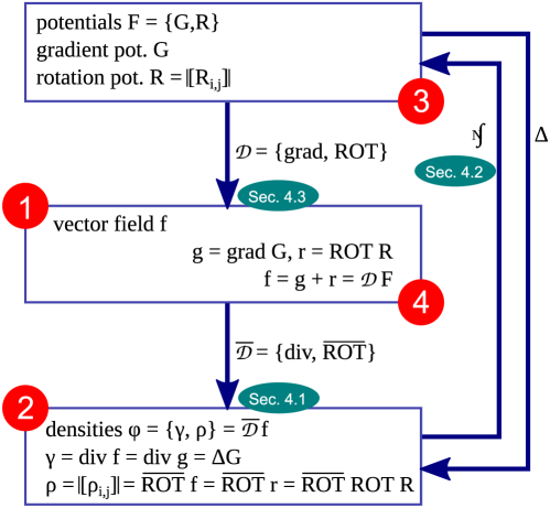
Figure 1: Relation between source density $\phi$, vector field $f$ and Newton potential $F$ in $\mathbb{R}^{n}$. To get the Helmholtz Decomposition of the vector field $f$, derive the densities applying the operator $\overline{\mathcal{D}}$ described in Sec. 4.1. These densities are convolved with the fundamental solutions of the Laplace equation to derive scalar and rotation potentials (using the ‘Newton potential operator ${}^{N}\!\!\!\!\int$’) as explained in Sec. 4.2. The gradient field $g$ and the rotation field $r$ that sum to the original field $f$ are derived using the operator $\mathcal{D}$ defined in Sec. 4.3.

In the following, we present a simpler approach to Helmholtz Decomposition of a twice continuously differentiable vector field $f(x)$ that decays faster than $|x|^{-c}$ for $|x|\to\infty$ and $c>0$. The basic idea is to understand the rotation in dimension $n$ as a combination of $\binom{n}{2}$ rotations within the planes spanned by two of the Cartesian coordinates. In each of these planes of rotation, applying the $\overline{\operatorname{curl}}$ in two dimensions is sufficient. These $\binom{n}{2}$ rotation densities form the upper triangle of a matrix. For tractability, we complete this to a $n\times n$ matrix by making it antisymmetric. It thus contains redundantly both the rotation in the $x_{i}$-$x_{j}$-plane and in the $x_{j}$-$x_{i}$-plane. Nevertheless, it has only $n^{2}$ entries, instead of $n^{n-2}$ entries for $\overline{\operatorname{curl}}$, and contains only the mutually different entries of this operator.

We proceed along the steps shown in Figure 1. Starting ❶ from $f$, we calculate ❷ the scalar source density $\gamma$ and $n^{2}$ basic rotation densities $\rho_{ij}$ using the new differential operator $\overline{\mathcal{D}}$, consisting of the well-known divergence $\operatorname{div}$ and the new operator $\overline{\operatorname{ROT}}$ (Sec. 4.1). Each basic rotation density $\rho_{ij}$ corresponds to the rotation within the $x_{i}$-$x_{j}$-plane. The basic rotation densities form the $n^{2}$-dimensional, antisymmetric rotation density $\rho=\left\llbracket\rho_{ij}\right\rrbracket=\overline{\operatorname{ROT}}f$ and together with $\gamma=\operatorname{div}f$ the density $\phi=\Big{\{}\gamma,\rho(x)\Big{\}}=\left\{\gamma,\left\llbracket\rho_{ij}\right\rrbracket\right\}$. The Newton potential operator ${}^{N}\!\!\!\!\int$ convolves these densities with the fundamental solutions of the Laplace equation, yielding ❸ the scalar ‘source potential’ $G={}^{N}\!\!\!\!\int\gamma$ and $n^{2}$ ‘basic rotation potentials’ $R_{ij}={}^{N}\!\!\!\!\int\rho_{ij}$ (Sec. 4.2). Similar to the densities, these $n^{2}$ scalar fields $R_{ij}$ can be jointly written as antisymmetric ‘rotation potential’ $R=\left\llbracket R_{ij}\right\rrbracket$. With a new differential operator $\mathcal{D}$, combining the well-known gradient $\operatorname{grad}$ with the new operator $\operatorname{ROT}$, operating on the potential $F=\big{\{}G,R\big{\}}$, a rotation-free ‘gradient field’ $g=\operatorname{grad}G$ and a source-free ‘rotation field’ $r=\operatorname{ROT}R$ can be calculated (Sec. 4.3). In sum ❹, they yield the original vector field $f(x)$.

4 Definitions

The notation is that square brackets $[f_{k}]$ indicate a vector, double square brackets $\llbracket R_{ij}\rrbracket$ a $n\times n$ matrix and curly brackets $\left\{\gamma,\llbracket\rho_{ij}\rrbracket\right\}$ an object of dimension $1+n^{2}$. For comparison, the table in the Appendix A summarizes the definitions and important properties of the operators and variables, and shows their similarities to the well-known decomposition in dimension 3.

Let $f\in C^{2}(\mathbb{R}^{n},\mathbb{R}^{n})$ be a twice continuously differentiable vector field that decays faster than $\left|x\right|^{-c}$ for $\left|x\right|\to\infty$ and $c>0$.

$$f(x)=\left[f_{k}(x);1\leq k\leq n\right]=\left[f_{1}(x),\dots,f_{n}(x)\right].$$ (8)

Definition 1 (Helmholtz Decomposition, gradient field and rotation field).

For a vector field $f\in C^{2}(\mathbb{R}^{n},\mathbb{R}^{n})$, a ‘gradient field’ $g\in C^{2}(\mathbb{R}^{n},\mathbb{R}^{n})$ and a ‘rotation field’ $r\in C^{2}(\mathbb{R}^{n},\mathbb{R}^{n})$ are called a ‘Helmholtz Decomposition of $f$’, if they sum to $f$, if $g$ is gradient of some ‘gradient potential’ $G$, and if $r$ is divergence-free:

$$f(x) =g(x)+r(x),$$ (9)

$$g(x) =\operatorname{grad}G(x),$$ (10)

$$0 =\operatorname{div}r(x).$$ (11)

4.1 From vector field to densities

To get from the vector field $f$ to the source and rotation densities, we start with the Jacobian Matrix $J$ of $f$ and its decomposition into a symmetric part $S$ and an antisymmetric part $A$:

$$J=\left\llbracket J_{ij}\right\rrbracket=\left\llbracket\frac{\partial f_{i}}{\partial x_{j}}\right\rrbracket=S+A\quad\text{ with }\quad S=\frac{J+J^{\top}}{2}\quad\text{ and }\quad A=\frac{J-J^{\top}}{2}.$$ (12)

Definition 2 (scalar source density $\gamma$).

Analogously to $\mathbb{R}^{3}$, we define the ‘scalar source density’ $\gamma\in C^{1}(\mathbb{R}^{n},\mathbb{R})$ for the vector field $f$ as trace of the Jacobian of $f$:

$$\gamma(x)\coloneqq\operatorname{Tr}J=\sum_{i=1}^{n}\frac{\partial f_{i}}{\partial x_{i}}=\operatorname{div}f(x).$$ (13)

Definition 3 (basic rotation density operator $\overline{\operatorname{ROT}_{ij}}$).

We define the ‘basic rotation density operator’ $\overline{\operatorname{ROT}_{ij}}\colon C^{1}(\mathbb{R}^{n},\mathbb{R}^{n})\to C^{0}(\mathbb{R}^{n},\mathbb{R})$ for $1\leq i,j\leq n$ of the vector field $f$ as $2$ times the i-j-element of the antisymmetric part $A$ of the Jacobian $J$:

$$\overline{\operatorname{ROT}_{ij}}f(x) =2A_{ij}=\frac{\partial f_{i}}{\partial x_{j}}-\frac{\partial f_{j}}{\partial x_{i}}.$$ (14)

This generalizes the two-dimensional $\overline{\operatorname{curl}}$ in the $x_{1}$-$x_{2}$-plane of Eq. (5) given by $\overline{\operatorname{curl}}f=\frac{\partial f_{2}}{\partial x_{1}}-\frac{\partial f_{1}}{\partial x_{2}}$ to the rotation in the $x_{i}$-$x_{j}$-plane, just with a different sign convention. To avoid confusion with $\overline{\operatorname{curl}}$, we use $\overline{\operatorname{ROT}}$ for rotation of vector fields – and later define $\operatorname{ROT}_{ij}$ analogously to $\operatorname{curl}$ without the overline operating on scalar fields.

Definition 4 (rotation density operator $\overline{\operatorname{ROT}}$).

The ‘rotation density operator’ $\overline{\operatorname{ROT}}\colon C^{1}(\mathbb{R}^{n},\mathbb{R}^{n})\to C^{0}(\mathbb{R}^{n},\mathbb{R}^{n^{2}})$ is defined as an antisymmetric operator containing all the basic rotation density operators:

$$\overline{\operatorname{ROT}}f(x)\coloneqq\left\llbracket\overline{\operatorname{ROT}_{ij}}f(x)\right\rrbracket=\left\llbracket\left(\frac{\partial f_{i}}{\partial x_{j}}-\frac{\partial f_{j}}{\partial x_{i}}\right);1\leq i,j\leq n\right\rrbracket.$$ (15)

Definition 5 (basic rotational densities $\rho_{ij}$).

We define the $n^{2}$ ‘basic rotational densities’ $\rho_{ij}\in C^{1}(\mathbb{R}^{n},\mathbb{R}^{n})$ for $1\leq i,j\leq n$ and the matrix $\rho\in C^{1}(\mathbb{R}^{n},\mathbb{R}^{n^{2}})$ containing these $n^{2}$ densities as the rotation density operators applied to the vector field $f$:

$$\rho_{ij}(x)\coloneqq \,\overline{\operatorname{ROT}_{ij}}f(x),$$ (16)

$$\rho(x)\coloneqq \left\llbracket\rho_{ij}(x)\right\rrbracket=\left\llbracket\rho_{ij}(x);1\leq i,j\leq n\right\rrbracket=\left\llbracket\overline{\operatorname{ROT}_{ij}}f(x);1\leq i,j\leq n\right\rrbracket=\overline{\operatorname{ROT}}f(x).$$ (17)

As $\overline{\operatorname{ROT}_{ij}}$ and $\rho_{ij}$ are antisymmetric, they in fact only contain $\binom{n}{2}$ independent elements, one for each of the $\binom{n}{2}$ coordinate planes.

Definition 6 (density derivative $\overline{\mathcal{D}}$, density $\phi$).

We define the ‘density derivative’ $\overline{\mathcal{D}}\colon C^{1}(\mathbb{R}^{n},\mathbb{R}^{n})\to C^{0}(\mathbb{R}^{n},\mathbb{R}^{1+n^{2}})$ of the vector field $f$ that combines $\operatorname{div}$ and $\operatorname{ROT}$ into one operator, and define the ‘density’ $\phi\in C^{1}(\mathbb{R}^{n},\mathbb{R}^{1+n^{2}})$ that combines the source and rotation densities:

$$\phi(x)\coloneqq\Big{\{}\gamma(x),\rho(x)\Big{\}}=\left\{\gamma(x),\left\llbracket\rho_{ij}(x)\right\rrbracket\right\}=\overline{\mathcal{D}}f(x)\coloneqq\left\{\operatorname{div}f(x),\overline{\operatorname{ROT}}f(x)\right\}.$$ (18)

4.2 From densities to potentials

The next step derives the potentials starting from the densities using the Newton potential operator.

Definition 7 (Newton potential operator ${}^{N}\!\!\!\!\int$).

We define the ‘Newton potential operator’ ${}^{N}\!\!\!\!\int\colon C^{0}(\mathbb{R}^{n},\mathbb{R})\to C^{2}(\mathbb{R}^{n},\mathbb{R})$ as convolution of any density $Q\in\{\phi,\gamma,\rho,\rho_{ij}\}$ that decays faster than $\left|x\right|^{-c}$ for $\left|x\right|\to\infty$ and $c>0$ with the fundamental solutions of the Laplace equation $\Delta K(x)=0$:

$${}^{N}\!\!\!\!\!\int Q(x)=\int_{\mathbb{R}^{n}}K(x,\xi)\ Q(\xi)\ d\xi^{n}$$ (19)

with the kernel $K(x,\xi)$, using $V_{n}=\pi^{\frac{n}{2}}/\Gamma\big{(}\tfrac{n}{2}+1\big{)}$ the volume of a unit $n$-ball and $\Gamma(x)$ the gamma function,

$$K(x,\xi) =\begin{cases}\frac{1}{2\pi}\left(\log{|x-\xi|}-\log{|\xi|}\right)&n=2,\\ \frac{1}{n(2-n)V_{n}}\left(|x-\xi|^{2-n}-|\xi|^{2-n}\right)&\text{otherwise},\end{cases}$$

We call a potential derived this way ‘Newton potential’. The decay of $Q$ at infinity guarantees the existence of the convolution integrals, similar to the 3-dimensional case, but the use of the more complex kernel compared to Eq. (2) allows to relax the restriction to fields decaying faster than $|x|^{-c}$ with $c>0$, instead of $c=2$ [2, 13].

Definition 8 (source potential $G$).

We define the one-dimensional ‘source potential’ $G\in C^{3}(\mathbb{R}^{n},\mathbb{R})$ as application of the Newton potential operator to the source density:

$$G(x) \coloneqq{}^{N}\!\!\!\!\!\int\gamma(x)\ \coloneqq\int_{\mathbb{R}^{n}}K(x,\xi)\ \gamma(\xi)\ d\xi^{n},$$ (20)

Note that compared to the case in $\mathbb{R}^{3}$, we use a different sign convention: $G(x)=-\Phi(x)$.

Definition 9 (basic rotation potentials $R_{ij}$).

We define $n^{2}$ ‘basic rotation potentials’ $R_{ij}\in C^{3}(\mathbb{R}^{n},\mathbb{R})\text{ for }1\leq i,j\leq n$, corresponding to the coordinate plane spanned by $x_{i}$ and $x_{j}$, as application of the Newton potential operator to the basic rotation densities:

$$R_{ij}(x) \coloneqq{}^{N}\!\!\!\!\!\int\rho_{ij}(x)=\int_{\mathbb{R}^{n}}K(x,\xi)\ \rho_{ij}(\xi)\ d\xi^{n}.$$ (21)

Definition 10 (rotation potential $R$).

We define the ‘rotation potential’ $R\in C^{3}(\mathbb{R}^{n},\mathbb{R}^{n^{2}})$ as matrix containing the $n^{2}$ basic rotation potentials $R_{ij}$:

$$R(x) \coloneqq\left\llbracket R_{ij}(x)\right\rrbracket=\left\llbracket R_{ij}(x);1\leq i,j\leq n\right\rrbracket=\left\llbracket{}^{N}\!\!\!\!\!\int\rho_{ij}(x);1\leq i,j\leq n\right\rrbracket={}^{N}\!\!\!\!\!\int\rho(x).$$ (22)

Here, the Newton potential operator ${}^{N}\!\!\!\!\int$ is applied in each component. The rotation potential $R(x)$ is antisymmetric, thus $R_{ij}(x)=-R_{ji}(x)$ and $R_{ii}(x)=0$, and the rotation potentials therefore contains $\binom{n}{2}$ distinct components.

Definition 11 (potential $F$).

The ‘potential’ $F\in C^{3}(\mathbb{R}^{n},\mathbb{R}^{1+n^{2}})$ combines source and rotation potentials into one object of dimension $1+n^{2}$:

$$F(x) \coloneqq\Big{\{}G(x),R(x)\Big{\}}={}^{N}\!\!\!\!\!\int\phi(x)={}^{N}\!\!\!\!\!\int\overline{\mathcal{D}}f(x).$$ (23)

We know from the theory of the Poisson equation [5] that $\Delta{}^{N}\!\!\!\!\int Q(x)=Q(x)$ for $Q\in C(\mathbb{R}^{n},\mathbb{R}^{m})$, which implies:

$$\Delta G(x)=\gamma(x),\qquad\Delta R_{ij}(x)=\rho_{ij}(x)\ \forall\ i,j,\qquad\Delta R(x)=\rho(x),\qquad\Delta F(x)=\phi(x).$$ (24)

4.3 From potentials to vector fields

Definition 12 (basic rotation operator $\operatorname{ROT}_{ij}$).

We define the ‘basic rotation operator’ $\operatorname{ROT}_{ij}\colon C^{1}(\mathbb{R}^{n},\mathbb{R})\to C^{0}(\mathbb{R}^{n},\mathbb{R}^{n})$ operating on the basic rotation potential $R_{ij}$ with $1\leq i,j\leq n$ as

$$\operatorname{ROT}_{ij}R_{ij}(x)\coloneqq \left[0,\dots,0,+\frac{\partial R_{ij}}{\partial x_{j}},0,\dots,0,-\frac{\partial R_{ij}}{\partial x_{i}},0,\dots,0\right]$$ (25)

$$= \left[\delta_{ik}\frac{\partial R_{ij}}{\partial x_{j}}-\delta_{jk}\frac{\partial R_{ij}}{\partial x_{i}};1\leq k\leq n\right],$$

with the Kronecker delta $\delta_{ik}=1$ if $i=k$ and $0$ otherwise.

This operator is a generalization of $\operatorname{curl}$ operating on a scalar field in the two-dimensional case of rotations within the $x_{1}$-$x_{2}$-plane in Eq. (4) given by $\left[\delta_{2k}\frac{\partial R}{\partial x_{1}}-\delta_{1k}\frac{\partial R}{\partial x_{2}};1\leq k\leq 2\right]$, again with a different sign convention. It operates in the $x_{i}$-$x_{j}$-plane, therefore the non-zero terms in this $n$-dimensional vector are located at positions $i$ and $j$, instead of $1$ and $2$ in the $2$-dimensional case. Note that $\operatorname{ROT}_{ij}R_{ij}(x)=\operatorname{ROT}_{ji}R_{ji}(x)$, yielding a symmetric object.

Definition 13 (rotation operator $\operatorname{ROT}$).

We define the ‘rotation operator’ $\operatorname{ROT}\colon C^{1}(\mathbb{R}^{n},\mathbb{R}^{n^{2}})\to C^{0}(\mathbb{R}^{n},\mathbb{R}^{n})$ for each rotation potential $R(x)=\left\llbracket R_{ij}(x)\right\rrbracket$ as superposition of the $\binom{n}{2}$ basic rotations in the coordinate planes. As the antisymmetric potential $R(x)$ of dimension $n^{2}$ contains each of the $\binom{n}{2}$ basic rotations twice, we have to devide the result by 2.

$$\operatorname{ROT}R(x)\coloneqq \frac{1}{2}\sum_{i,j=1}^{n}\operatorname{ROT}_{ij}R_{ij}(x)=\left[\sum_{m=1}^{n}\frac{\partial R_{km}}{\partial x_{m}};1\leq k\leq n\right].$$ (26)

Note that this is identical to $\operatorname{div}R_{km}$ for an antisymmetric second-rank tensor.

Definition 14 (gradient field $g$ and rotation field $r$).

The ‘gradient field’ $g\in C^{2}(\mathbb{R}^{n},\mathbb{R}^{n})$ and the ‘rotation field’ $r\in C^{2}(\mathbb{R}^{n},\mathbb{R}^{n})$ are defined as:

$$g(x) =\operatorname{grad}G(x),\qquad r(x)=\operatorname{ROT}R(x).$$ (27)

Definition 15 (derivative of the potential $\mathcal{D}$).

We define the ‘derivative of the potential’ $\mathcal{D}\colon C^{1}(\mathbb{R}^{n},\mathbb{R}^{1+n^{2}})\to C^{0}(\mathbb{R}^{n},\mathbb{R}^{n})$ operating on a potential $F(x)=\{G(x),R(x)\}$ as the sum of the gradient operating on the source potential $G(x)$ and the rotation operator $\operatorname{ROT}$ operating on the rotation potential $R(x)$:

$$\mathcal{D}F(x) =\mathcal{D}\Big{\{}G(x),R(x)\Big{\}}\coloneqq\operatorname{grad}G(x)+\operatorname{ROT}R(x)=g(x)+r(x).$$ (28)

We call a potential $F=\{G,R\}$ ‘antiderivative’ of $f$ if $f(x)=\mathcal{D}F(x)$.

Given the conditions on $f(x)$, the potential is uniquely determined by Eq. (20). We will prove that Eqs. (27) and (28) are a Helmholtz Decomposition according to Definition 1.

5 Helmholtz Decomposition Theorem

Theorem 1 (Helmholtz Decomposition Theorem).

Any twice continuously differentiable vector field $f\in C^{2}(\mathbb{R}^{n},\mathbb{R}^{n})$ that decays faster than $|x|^{-c}$ for $\left|x\right|\to\infty$ and $c>0$ can be decomposed into two vector fields, one rotation-free and one divergence-free. With the definitions of the operators in Section 4, let

$$G \in C^{3}(\mathbb{R}^{n},\mathbb{R}), \text{ \ \ with }G(x) \coloneqq{}^{N}\!\!\!\!\int\operatorname{div}f(x),$$ (29)

$$g \in C^{2}(\mathbb{R}^{n},\mathbb{R}^{n}), \text{ with }\ g(x) \coloneqq\operatorname{grad}G(x),$$ (30)

$$R \in C^{3}(\mathbb{R}^{n},\mathbb{R}^{n^{2}}), \text{ with }R(x) \coloneqq{}^{N}\!\!\!\!\int\overline{\operatorname{ROT}}f(x),$$ (31)

$$r \in C^{2}(\mathbb{R}^{n},\mathbb{R}^{n}), \text{ with }\ r(x) \coloneqq\operatorname{ROT}R(x),$$ (32)

then

$$g G 0 =\overline{\operatorname{ROT}}g(x)=\overline{\operatorname{ROT}}\operatorname{grad}G(x),$$, the gradient of , is rotation-free: (33)

$$r R 0 =\operatorname{div}r(x)=\operatorname{div}\operatorname{ROT}R(x),$$, the rotation of , is divergence-free: (34)

the potential $$\{G,R\} f f(x) =\mathcal{D}\big{\{}G(x),R(x)\big{\}},$$ is an antiderivative of : (35)

the Helmholtz Decomposition of $$f f(x) =g(x)+r(x).$$ is given by: (36)

Proof.

Propositions 2 and 3 show that $g(x)$ is curl-free and $r(x)$ is divergence-free (Eqs. 33–34). We introduce and prove Lemma 4, Corollary 5 and three operator identities as Propositions 6–8. In Proposition 9, we prove the conditions in Eqs. (35–36) that $g(x)+r(x)=\mathcal{D}F(x)$ equals the original vector field $f(x)$. ∎

Proposition 2 (Eq. (33) of the Helmholtz Decomposition Theorem: $g(x)=\operatorname{grad}G(x)$ is rotation-free).

For any twice continuously differentiable vector field $f\in C^{2}(\mathbb{R}^{n},\mathbb{R}^{n})$ that decays faster than $\left|x\right|^{-c}$ for $\left|x\right|\to\infty$ and $c>0$, the source potential $G(x)={}^{N}\!\!\!\!\int\operatorname{div}f(x)$ as defined by Eq. (20) and its gradient $g(x)=\operatorname{grad}G(x)$ satisfy the following identities:

$$\overline{\operatorname{ROT}}g(x) =\overline{\operatorname{ROT}}\operatorname{grad}G(x)=0,$$ (37)

$$\overline{\operatorname{curl}}g(x) =\overline{\operatorname{curl}}\operatorname{grad}G(x)=0.$$ (38)

Proof.

Using the Definition 4 of $\overline{\operatorname{ROT}}$ in Eq. (15) and of the components of $\overline{\operatorname{curl}}$ in Eq. (7), and permutability of second derivatives:

$$\begin{split}\overline{\operatorname{ROT}}g(x)&=\overline{\operatorname{ROT}}\operatorname{grad}G(x)=\overline{\operatorname{ROT}}\left[\frac{\partial G}{\partial x_{1}},\dots,\frac{\partial G}{\partial x_{n}}\right]\\ &=\left\llbracket\frac{\partial}{\partial x_{i}}\frac{\partial G}{\partial x_{j}}-\frac{\partial}{\partial x_{j}}\frac{\partial G}{\partial x_{i}};1\leq i,j\leq n\right\rrbracket=0,\end{split}$$ (39)

$$\begin{split}\left(\overline{\operatorname{curl}}g(x)\right)_{e_{1},\dots,e_{n-2}}&=\sum_{1\leq i,j\leq n}\tfrac{1}{2}\epsilon_{e_{1},\dots,e_{n-2},i,j}\cdot\left(\frac{\partial g_{i}}{\partial x_{j}}-\frac{\partial g_{j}}{\partial x_{i}}\right)\\ &=\sum_{1\leq i,j\leq n}\tfrac{1}{2}\epsilon_{e_{1},\dots,e_{n-2},i,j}\cdot\left(\frac{\partial}{\partial x_{j}}\frac{\partial G}{\partial x_{i}}-\frac{\partial}{\partial x_{i}}\frac{\partial G}{\partial x_{j}}\right)=0.\end{split}$$ (40)

∎

Proposition 3 (Eq. (34) of the Helmholtz Decomposition Theorem: $r(x)=\operatorname{ROT}R(x)$ is divergence-free).

For any twice continuously differentiable vector field $f\in C^{2}(\mathbb{R}^{n},\mathbb{R}^{n})$ that decays faster than $\left|x\right|^{-c}$ for $\left|x\right|\to\infty$ and $c>0$, the rotation potential $R(x)={}^{N}\!\!\!\!\int\overline{\operatorname{ROT}}f(x)$ as defined by Eqs. (21) and (22) and its rotation $r(x)=\operatorname{ROT}R(x)$ satisfy the following identity:

$$\operatorname{div}r(x)=\operatorname{div}\operatorname{ROT}R(x)=0$$ (41)

Proof.

Using definition of $\operatorname{ROT}$ in Eq. (26) and $\operatorname{ROT}_{ij}$ in Eq. (25), exchangeability of derivatives and sums, and permutability of second derivatives:

$$\begin{split}\operatorname{div}\operatorname{ROT}_{ij}R_{ij}(x)=&\operatorname{div}\left[\delta_{ik}\frac{\partial R_{ij}}{\partial x_{j}}-\delta_{jk}\frac{\partial R_{ij}}{\partial x_{i}};1\leq k\leq n\right]\\ =&\sum_{k=1}^{n}\frac{\partial}{\partial x_{k}}\left(\delta_{ik}\frac{\partial R_{ij}}{\partial x_{j}}-\delta_{jk}\frac{\partial R_{ij}}{\partial x_{i}}\right)=\sum_{k=1}^{n}\left(\frac{\partial^{2}R_{ij}}{\partial x_{i}\partial x_{j}}-\frac{\partial^{2}R_{ij}}{\partial x_{j}\partial x_{i}}\right)=0.\end{split}$$ (42)

$$\begin{split}\operatorname{div}r(x)=&\operatorname{div}\operatorname{ROT}R(x)=\operatorname{div}\sum_{i,j}^{n}\tfrac{1}{2}\operatorname{ROT}_{ij}R_{ij}(x)\\ =&\tfrac{1}{2}\sum_{i,j}^{n}\operatorname{div}\operatorname{ROT}_{ij}R_{ij}(x)=\sum_{i,j}^{n}0=0.\end{split}$$ (43)

∎

Lemma 4 (Exchangeablity of the Newton potential operator with any partial derivative).

For any continuously differentiable vector field $Q\in C^{1}(\mathbb{R}^{n},\mathbb{R}^{m})$ that decays faster than $\left|x\right|^{-c}$ for $\left|x\right|\to\infty$ and $c>0$, the Newton potential operator as defined by Eq. (20) can be exchanged with any partial derivative:

$$\dfrac{\partial}{\partial x_{k}}{}^{N}\!\!\!\!\!\int Q(x) ={}^{N}\!\!\!\!\!\int\frac{\partial Q(x)}{\partial x_{k}}.$$ (44)

In the context of this paper, $Q$ can be $G$, $R$, $R_{ij}$, $F$, $f$, $g$, $r$, $\gamma$, $\rho$, $\rho_{ij}$, or $\phi$.

Proof.

$$\begin{split}\frac{\partial}{\partial x_{k}}{}^{N}\!\!\!\!\!\int Q(x)&=\frac{\partial}{\partial x_{k}}\int_{\mathbb{R}^{n}}K(x,\xi)Q(\xi)\,d\xi^{n}=\int_{\mathbb{R}^{n}}Q(\xi)\left(\frac{\partial}{\partial x_{k}}K(x,\xi)\right)\,d\xi^{n}\\ &=\int_{\mathbb{R}^{n}}Q(\xi)\left(-\frac{\partial}{\partial\xi_{k}}K(x,\xi)\right)\,d\xi^{n}\end{split}$$ (45)

using integration by parts in the $$k$$-component

$$=-\int_{\mathbb{R}^{n-1}}\left(Q(\xi)K(x,\xi)\Big{|}_{\xi_{k}=-\infty}^{\infty}-\int_{\xi_{k}=-\infty}^{\infty}\frac{\partial Q(\xi)}{\partial\xi_{k}}K(x,\xi)\,d\xi_{k}\right)\,d[\xi_{i};i\neq k]$$ (46)

(for $$n=1 \mathbb{R}^{0} Q(\xi)K(x,\xi)\to 0 \xi_{k}\to\pm\infty$$, the outer integral over in the intermediate step above is omitted) and as in the first summand for

$$=\int_{\mathbb{R}^{n}}\frac{\partial Q(\xi)}{\partial\xi_{k}}K(x,\xi)\,d\xi^{n}={}^{N}\!\!\!\!\!\int\left(\frac{\partial Q(x)}{\partial x_{k}}\right)\ \forall\ k.$$ (47)

∎

Corollary 5.

Applying Lemma 4 in each component, it follows

$${}^{N}\!\!\!\!\int\Delta Q(x) =\Delta{}^{N}\!\!\!\!\int Q(x)=Q(x) \textup{ for }Q\in C^{2}(\mathbb{R}^{n},\mathbb{R}^{m}),$$ (48)

$$\mathcal{D}\,{}^{N}\!\!\!\!\int F(x) ={}^{N}\!\!\!\!\int\mathcal{D}F(x) \textup{ for a potential }F\in C^{3}(\mathbb{R}^{n},\mathbb{R}^{1+n^{2}}),$$ (49)

$$\textup{and }\quad\overline{\mathcal{D}}\,{}^{N}\!\!\!\!\int f(x) ={}^{N}\!\!\!\!\int\overline{\mathcal{D}}f(x) \textup{ for a vector field }f\in C^{2}(\mathbb{R}^{n},\mathbb{R}^{n}).$$ (50)

Proposition 6 (Operator Identity: $\mathcal{D}\overline{\mathcal{D}}f=\Delta f$).

For any twice continuously differentiable vector field $f\in C^{2}(\mathbb{R}^{n},\mathbb{R}^{n})$, the following identity holds:

$$\mathcal{D}\overline{\mathcal{D}}f(x)=\operatorname{grad}\operatorname{div}f(x)+\operatorname{ROT}\overline{\operatorname{ROT}}f(x)=\Delta f(x).$$ (51)

Proof.

The first part follows from the definition of $\mathcal{D}$ and $\overline{\mathcal{D}}$, and Proposition 2 and 3. By using Eq. (26) stating $\operatorname{ROT}R(x)=\left[\sum_{m}\frac{\partial R_{km}}{\partial x_{m}};1\leq k\leq n\right]$, it follows:

$$\begin{split}\mathcal{D}\overline{\mathcal{D}}f(x)&=\operatorname{grad}\operatorname{div}f+\operatorname{ROT}\left\llbracket\left(\frac{\partial f_{i}}{\partial x_{j}}-\frac{\partial f_{j}}{\partial x_{i}}\right);1\leq i,j\leq n\right\rrbracket\\ &=\left[\frac{\partial}{\partial x_{k}}\sum_{m=1}^{n}\frac{\partial f_{m}}{\partial x_{m}}+\sum_{m=1}^{n}\frac{\partial}{\partial x_{m}}\left(\frac{\partial f_{k}}{\partial x_{m}}-\frac{\partial f_{m}}{\partial x_{k}}\right);1\leq k\leq n\right]\\ &=\left[\sum_{m=1}^{n}\frac{\partial^{2}f_{k}}{\partial x_{m}^{2}};1\leq k\leq n\right]=\left[\Delta f_{k};1\leq k\leq n\right]=\Delta f(x).\end{split}$$ (52)

The first two terms cancel out because of the symmetry of second derivatives (Schwarz’s theorem) and interchange of sum and derivative. ∎

Proposition 7 (Operator Identity: $(-1)^{n}\operatorname{curl}\overline{\operatorname{curl}}f=\operatorname{ROT}\overline{\operatorname{ROT}}f$).

For any twice continuously differentiable vector field $f\in C^{2}(\mathbb{R}^{n},\mathbb{R}^{n})$, the following identity holds:

$$(-1)^{n}\operatorname{curl}\overline{\operatorname{curl}}f(x) =\operatorname{ROT}\overline{\operatorname{ROT}}f(x).$$ (53)

Proof.

This follows from Proposition 6 and the well-known identity [4, p. 522]

$$\Delta f(x)=\operatorname{grad}\operatorname{div}f(x)+(-1)^{n}\operatorname{curl}\overline{\operatorname{curl}}f(x).$$ (54)

∎

Proposition 8 (Identity for Newton Potential $F$: $\overline{\mathcal{D}}\mathcal{D}F=\Delta F$).

For any twice continuously differentiable vector field $f\in C^{2}(\mathbb{R}^{n},\mathbb{R}^{n})$ that decays faster than $\left|x\right|^{-c}$ for $\left|x\right|\to\infty$ and $c>0$, the potential $F(x)={}^{N}\!\!\!\!\int\overline{\mathcal{D}}f(x)$ as defined by Eqs. (18) and (23) satisfies the following identity:

$$\overline{\mathcal{D}}\mathcal{D}F(x)=\Delta F(x).$$ (55)

Proof.

Using the definition of $F(x)$, Corollary 5 stating ${}^{N}\!\!\!\!\int\overline{\mathcal{D}}f(x)=\overline{\mathcal{D}}\,{}^{N}\!\!\!\!\int f(x)$, Proposition 6 stating $\mathcal{D}\overline{\mathcal{D}}=\Delta$, the definition of $\phi(x)$ in Eq. (18), and $\Delta F(x)=\phi(x)$ from Eq. (24):

$$\overline{\mathcal{D}}\mathcal{D}F(x)=\overline{\mathcal{D}}\mathcal{D}\,{}^{N}\!\!\!\!\!\int\overline{\mathcal{D}}f(x)=\overline{\mathcal{D}}\mathcal{D}\overline{\mathcal{D}}\,{}^{N}\!\!\!\!\!\int f(x)=\overline{\mathcal{D}}\Delta{}^{N}\!\!\!\!\!\int f(x)=\overline{\mathcal{D}}f(x)=\phi(x)=\Delta F(x).$$ (56)

∎

Note: While Proposition 6 is an operator identity for any field $f(x)$, this derivation is valid only if $F(x)$ was constructed following Eqs. (18) and (23). For a general function $Q\in C^{3}(\mathbb{R}^{n},\mathbb{R}^{1+n^{2}})$, $\overline{\mathcal{D}}\mathcal{D}Q(x)$ may differ from $\Delta Q(x)$.

Proposition 9 (Eqs. (35–36) of the Helmholtz Decomposition Theorem: $g(x)+r(x)=f(x)$).

For any twice continuously differentiable vector field $f\colon\mathbb{R}^{n}\to\mathbb{R}^{n}$ that decays faster than $\left|x\right|^{-c}$ for $\left|x\right|\to\infty$ and $c>0$, the source potential $G(x)={}^{N}\!\!\!\!\int\operatorname{div}f(x)$ as defined by Eq. (20) and its gradient $g(x)=\operatorname{grad}G(x)$, the rotation potential $R(x)={}^{N}\!\!\!\!\int\overline{\operatorname{ROT}}f(x)$ as defined by Eqs. (21) and (22) and its rotation $r(x)=\operatorname{ROT}R(x)$, and the potential $F(x)=\{G(x),R(x)\}$ as defined by Eq. (23) satisfy the following identity:

$$g(x)+r(x)=\operatorname{grad}G(x)+\operatorname{ROT}R(x)=\mathcal{D}F(x)=f(x).$$ (57)

Proof.

The first equalities follow immediately from the definitions. The last can be derived starting with the definition of $F(x)$, applying Corollary 5 and Proposition 6:

$$\mathcal{D}F(x)=\mathcal{D}\,{}^{N}\!\!\!\!\!\int\overline{\mathcal{D}}f(x)=\mathcal{D}\overline{\mathcal{D}}\,{}^{N}\!\!\!\!\!\int f(x)=\Delta{}^{N}\!\!\!\!\!\int f(x)=f(x).$$ (58)

∎

This completes the proof of the Helmholtz Decomposition Theorem.

6 Conclusions

In this paper, we have introduced differential operators $\overline{\operatorname{ROT}}$, $\operatorname{ROT}$ and the generalized derivatives $\overline{\mathcal{D}}$ and $\mathcal{D}$, such that for any twice continuously differentiable vector field $f(x)$ in $\mathbb{R}^{n}$ that decays faster then $\left|x\right|^{-c}$ for $x\to\infty$ and $c>0$, a scalar source potential $G(x)$ and an antisymmetric rotation potential $R(x)=R_{ij}(x)$ with $\binom{n}{2}$ distinct entries can be calculated as convolutions of the density $\phi(x)=\overline{\mathcal{D}}f(x)$ with the fundamental solutions of the Laplace equation. The joint potential $F(x)=\left\{G(x),R(x)\right\}$ is an antiderivative of $f(x)$, such that applying the differential operator $\mathcal{D}$ to this potential provides a decomposition of $f(x)$ into a rotation-free ‘gradient field’ $g(x)=\operatorname{grad}G(x)$ and a source-free ‘rotation field’ $r(x)=\operatorname{ROT}R(x)$:

$$f(x) =\mathcal{D}F(x)=\mathcal{D}\,{}^{N}\!\!\!\!\int\overline{\mathcal{D}}f(x)=\mathcal{D}\,{}^{N}\!\!\!\!\!\int\phi(x)=g(x)+r(x).$$ (59)

This generalizes the Helmholtz Decomposition to $\mathbb{R}^{n}$ without the need for differential forms and the complicated operator $\operatorname{curl}$ and facilitates its application to high-dimensional dynamic systems. The potentials correspond to ‘antiderivatives’ of the gradient and rotation differential operators, providing a generalization of the fundamental theorem of calculus in $\mathbb{R}^{n}$ that links differential and integral calculus.

Appendix A Comparison of the Helmholtz Decomposition, operators and variables in dimension n with dimension 3

Variable or operator	dimension n	dimension 3
source potential $G\in C^{3}(\mathbb{R}^{n},\mathbb{R})$	$\displaystyle G(x)$	$\displaystyle\Phi(x)=-G(x)$ (60)
basic rotation potentials $R_{ij},R_{i}\in C^{3}(\mathbb{R}^{n},\mathbb{R})$	$\displaystyle R_{ij}(x)=-R_{ji}(x);1\leq i,j\leq n,\qquad\tbinom{n}{2}\text{ distinct entries }$	$\displaystyle R_{1},R_{2},R_{3},\qquad\tbinom{n}{2}=3\text{ distinct entries}$ (61)
rotation potential $R\in C^{3}(\mathbb{R}^{n},\mathbb{R}^{n^{2}})$	$\displaystyle R(x)=\left\llbracket R_{ij}(x);1\leq i,j\leq n\right\rrbracket\qquad n\times n\text{ matrix}$	$\displaystyle R(x)=A(x)=\left[R_{1},R_{2},R_{3}\right]$ (62)
potential $F\in C^{3}(\mathbb{R}^{n},\mathbb{R}^{1+n^{2}})$	$\displaystyle F(x)=\Big{\{}G(x),R(x)\Big{\}}$	$\displaystyle F(x)=\Big{\{}G(x),R(x)\Big{\}}$ (63)
basic rotation operator $\operatorname{ROT}_{ij}\colon C^{1}(\mathbb{R}^{n},\mathbb{R})\to C^{0}(\mathbb{R}^{n},\mathbb{R}^{n})$	$\displaystyle\operatorname{ROT}_{ij}R_{ij}\coloneqq\left[\delta_{ik}\frac{\partial R_{ij}}{\partial x_{j}}-\delta_{jk}\frac{\partial R_{ij}}{\partial x_{i}};1\leq k\leq n\right]$
rotation operator $\operatorname{ROT}R\colon C^{1}(\mathbb{R}^{n},\mathbb{R}^{n^{2}})\to C^{0}(\mathbb{R}^{n},\mathbb{R}^{n})$	$\displaystyle\operatorname{ROT}R\coloneqq$ $\displaystyle\sum_{1\leq i,j\leq n}\tfrac{1}{2}\operatorname{ROT}_{ij}R_{ij}=\left[\sum_{m}\frac{\partial R_{km}}{\partial x_{m}};1\leq k\leq n\right]$	$\displaystyle\operatorname{curl}R=\left[\frac{\partial R_{3}}{\partial x_{2}}-\frac{\partial R_{2}}{\partial x_{3}},\ \frac{\partial R_{1}}{\partial x_{3}}-\frac{\partial R_{3}}{\partial x_{1}},\ \frac{\partial R_{2}}{\partial x_{1}}-\frac{\partial R_{1}}{\partial x_{2}}\right]$ (65)
	$\operatorname{ROT}R=\operatorname{curl}R$ with $R_{1}=R_{23}$; $R_{2}=-R_{13}$; $R_{3}=+R_{1,2}\quad$
vector field $f$, gradient field $g$ and rotation field $r$ $f,g,r\in C^{2}(\mathbb{R}^{n},\mathbb{R}^{n})$	$\displaystyle f(x)$ $\displaystyle=g(x)+r(x)$ $\displaystyle g(x)$ $\displaystyle=\operatorname{grad}G(x);\quad r(x)=\operatorname{ROT}R(x)$	$\displaystyle f(x)$ $\displaystyle=g(x)+r(x)$ (66) $\displaystyle g(x)$ $\displaystyle=\operatorname{grad}G(x);\quad r(x)=\operatorname{curl}R(x)$ (67)
gradient fields are rotation-free	$\displaystyle\overline{\operatorname{ROT}}g(x)=\overline{\operatorname{ROT}}\operatorname{grad}G(x)=0$	$\displaystyle\overline{\operatorname{curl}}g(x)=\overline{\operatorname{curl}}\operatorname{grad}G(x)=0$ (68)
rotational fields are divergence-free	$\displaystyle\operatorname{div}r(x)=\operatorname{div}\operatorname{ROT}R(x)=0$	$\displaystyle\operatorname{div}r(x)=\operatorname{div}\operatorname{curl}R(x)=0$ (69)
derivative of a potential $\mathcal{D}\colon C^{1}(\mathbb{R}^{n},\mathbb{R}^{1+n^{2}})\to C^{0}(\mathbb{R}^{n},\mathbb{R}^{n})$	$\displaystyle f(x)=\mathcal{D}F(x)\coloneqq\operatorname{grad}G(x)+\operatorname{ROT}R(x)$	$\displaystyle f(x)=\mathcal{D}F(x)\coloneqq-\operatorname{grad}\Phi(x)+\operatorname{curl}R(x)$ (70)
scalar source density $\gamma$ $\gamma\in C^{1}(\mathbb{R}^{n},\mathbb{R})$	$\displaystyle\gamma(x)=\operatorname{div}f(x)=\Delta G(x)$	$\displaystyle\gamma(x)=\operatorname{div}f(x)=\Delta G(x)$ (71)
basic rotation density op. $\overline{\operatorname{ROT}_{ij}}\colon C^{1}(\mathbb{R}^{n},\mathbb{R}^{n})\to C^{0}(\mathbb{R}^{n},\mathbb{R})$	$\displaystyle\overline{\operatorname{ROT}_{ij}}f(x)\coloneqq\left(\frac{\partial f_{i}}{\partial x_{j}}-\frac{\partial f_{j}}{\partial x_{i}}\right)$
rotation density operator $\overline{\operatorname{ROT}}\colon C^{1}(\mathbb{R}^{n},\mathbb{R}^{n})\to C^{0}(\mathbb{R}^{n},\mathbb{R}^{n^{2}})$	$\displaystyle\overline{\operatorname{ROT}}f(x)\coloneqq\left\llbracket\overline{\operatorname{ROT}_{ij}}f(x)\right\rrbracket=\left\llbracket\left(\frac{\partial f_{i}}{\partial x_{j}}-\frac{\partial f_{j}}{\partial x_{i}}\right);1\leq i,j\leq n\right\rrbracket$	$\displaystyle\overline{\operatorname{curl}}f=\left[\frac{\partial f_{3}}{\partial x_{2}}-\frac{\partial f_{2}}{\partial x_{3}},\ \frac{\partial f_{1}}{\partial x_{3}}-\frac{\partial f_{3}}{\partial x_{1}},\ \frac{\partial f_{2}}{\partial x_{1}}-\frac{\partial f_{1}}{\partial x_{2}}\right]$ (73)
basic rotation density $\rho_{ij},\rho_{i}\in C^{1}(\mathbb{R}^{n},\mathbb{R})$	$\displaystyle\rho_{ij}(x)=-\rho_{ji}(x)=\overline{\operatorname{ROT}_{ij}}f(x);1\leq i,j\leq n,$ $\displaystyle\tbinom{n}{2}\text{ distinct entries}$	$\displaystyle\rho_{1}(x),\rho_{2}(x),\rho_{3}(x)$ (74) $\displaystyle\tbinom{n}{2}=3\text{ distinct entries}$ (75)
rotation density $\rho$ $\rho\in C^{1}(\mathbb{R}^{n},\mathbb{R}^{n^{2}})$	$\displaystyle\rho(x)=\left\llbracket\rho_{ij}(x);1\leq i,j\leq n\right\rrbracket=\overline{\operatorname{ROT}}f(x)=\overline{\operatorname{ROT}}\operatorname{ROT}R$ $n\times n$ matrix	$\displaystyle\rho(x)=\left[\rho_{1},\rho_{2},\rho_{3}\right]=\overline{\operatorname{curl}}f(x)=\overline{\operatorname{curl}}\operatorname{curl}R(x)$ (76)       identify: $\rho_{1}=-\rho^{2,3}$; $\rho_{2}=+\rho^{1,3}$; $\rho_{3}=-\rho^{1,2}$
density derivative $\overline{\mathcal{D}}\colon C^{1}(\mathbb{R}^{n},\mathbb{R}^{n})\to C^{0}(\mathbb{R}^{n},\mathbb{R}^{1+n^{2}})$	$\displaystyle\overline{\mathcal{D}}f(x)\coloneqq\left\{\operatorname{div}f(x),\overline{\operatorname{ROT}}f(x)\right\}$	$\displaystyle\overline{\mathcal{D}}f(x)\coloneqq\left\{\operatorname{div}f(x),\overline{\operatorname{curl}}f(x)\right\}$ (77)
density $\phi\in C^{1}(\mathbb{R}^{n},\mathbb{R}^{1+n^{2}})$	$\displaystyle\phi(x)=\big{\{}\gamma(x),\rho(x)\big{\}}=\left\{\gamma(x),\left\llbracket\rho_{ij}(x)\right\rrbracket\right\}=\overline{\mathcal{D}}f(x)$	$\displaystyle\phi(x)=\big{\{}\gamma(x),\rho(x)\big{\}}=\left\{\gamma(x),\left[\rho_{1}(x),\rho_{2}(x),\rho_{3}(x)\right]\right\}=\overline{\mathcal{D}}f(x)$ (78)
Newton potential operator ${}^{N}\!\!\!\!\int\colon C^{0}(\mathbb{R}^{n},\mathbb{R})\to C^{2}(\mathbb{R}^{n},\mathbb{R})$	$\displaystyle G(x)$ $\displaystyle={}^{N}\!\!\!\!\!\int\gamma(x)=\int_{\mathbb{R}^{n}}K(x,\xi)\ \gamma(\xi)\ d\xi^{n}$ $\displaystyle R_{ij}(x)$ $\displaystyle={}^{N}\!\!\!\!\!\int\rho_{ij}(x)=\int_{\mathbb{R}^{n}}K(x,\xi)\ \rho_{ij}(\xi)\ d\xi^{n}$	$\displaystyle\Phi(x)$ $\displaystyle=\frac{1}{4\pi}\iiint_{\mathbb{R}^{3}}\frac{\gamma(\xi)}{|x-\xi|}\,d\xi^{3}$ (79) $\displaystyle R(x)$ $\displaystyle=\frac{1}{4\pi}\iiint_{\mathbb{R}^{3}}\frac{\rho(\xi)}{|x-\xi|}\,d\xi^{3}$ (80)
with the kernel $K(x,\xi)=\begin{cases}\frac{1}{2\pi}(\log{|x-\xi|}-\log{|\xi|})&n=2\\ \frac{1}{n(2-n)V_{n}}(|x-\xi|^{2-n}-|\xi|^{2-n})&n\neq 2,\text{ and }V_{n}=\pi^{\frac{n}{2}}/\Gamma\big{(}\tfrac{n}{2}+1\big{)}\text{ the volume of a unit $n$-ball, }V_{3}=4\pi/3\end{cases}$

References

- [1] Harsh Bhatia, Gregory Norgard, Valerio Pascucci and Peer-Timo Bremer “The Helmholtz-Hodge Decomposition—A Survey” In IEEE Transactions on Visualization and Computer Graphics 19.8, 2013, pp. 1386–1404 DOI: 10.1109/tvcg.2012.316
- [2] Otto Blumenthal “Über die Zerlegung unendlicher Vektorfelder” In Mathematische Annalen 61.2, 1905, pp. 235–250 DOI: 10.1007/BF01457564
- [3] George Dassios and Ismo V. Lindell “Uniqueness and reconstruction for the anisotropic Helmholtz decomposition” In Journal of Physics A: Mathematical and General 35.24, 2002, pp. 5139–5146 DOI: 10.1088/0305-4470/35/24/311
- [4] Bernardo De La Calle Ysern and José C. Sabina De Lis “A Constructive Proof of Helmholtz’s Theorem” In The Quarterly Journal of Mechanics and Applied Mathematics 72.4, 2019, pp. 521–533 DOI: 10.1093/qjmam/hbz016
- [5] David Gilbarg and Neil S. Trudinger “Elliptic Partial Differential Equations of Second Order” 224, Grundlehren der mathematischen Wissenschaften Heidelberg: Springer, 1977 DOI: 10.1007/978-3-642-96379-7
- [6] Erhard Glötzl and Oliver Richters “Analytical Helmholtz Decomposition and Potential Functions for many n-dimensional unbounded vector fields”, 2021 arXiv: https://arxiv.org/abs/2102.09556
- [7] Carlo Andrea Gonano and Riccardo Enrico Zich “Cross product in N Dimensions - the doublewedge product”, 2014 arXiv: https://arxiv.org/abs/1408.5799v1
- [8] Walter Hauser “On the Fundamental Equations of Electromagnetism” In American Journal of Physics 38.1, 1970, pp. 80–85 DOI: 10.1119/1.1976233
- [9] Hermann Helmholtz “Über Integrale der hydrodynamischen Gleichungen, welche den Wirbelbewegungen entsprechen.” In Journal für die reine und angewandte Mathematik 55, 1858, pp. 25–55 DOI: 10.1515/crll.1858.55.25
- [10] Alp Kustepeli “On the Helmholtz Theorem and Its Generalization for Multi-Layers” In Electromagnetics 36.3, 2016, pp. 135–148 DOI: 10.1080/02726343.2016.1149755
- [11] A.. McDavid and C.. McMullen “Generalizing Cross Products and Maxwell’s Equations to Universal Extra Dimensions”, 2006 arXiv: https://arxiv.org/abs/hep-ph/0609260v4
- [12] Dagmar Medková “The Laplace Equation” Cham: Springer International Publishing, 2018 DOI: 10.1007/978-3-319-74307-3
- [13] Dietmar Petrascheck “The Helmholtz decomposition revisited” In European Journal of Physics 37.1, 2015, pp. 015201 DOI: 10.1088/0143-0807/37/1/015201
- [14] Wolfgang Sprössig “On Helmholtz decompositions and their generalizations-An overview” In Mathematical Methods in the Applied Sciences 33.4, 2009, pp. 374–383 DOI: 10.1002/mma.1212
- [15] George Gabriel Stokes “On the Dynamical Theory of Diffraction” In Transactions of the Cambridge Philosophical Society 9, 1849, pp. 1–62 DOI: 10.1017/cbo9780511702259.015
- [16] Tomoharu Suda “Construction of Lyapunov functions using Helmholtz–Hodge decomposition” In Discrete & Continuous Dynamical Systems - A 39.5, 2019, pp. 2437–2454 DOI: 10.3934/dcds.2019103
- [17] Tomoharu Suda “Application of Helmholtz–Hodge decomposition to the study of certain vector fields” In Journal of Physics A: Mathematical and Theoretical 53.37, 2020, pp. 375703 DOI: 10.1088/1751-8121/aba657
- [18] Ton Tran-Cong “On Helmholtz’s Decomposition Theorem and Poissons’s Equation with an Infinite Domain” In Quarterly of Applied Mathematics 51.1, 1993, pp. 23–35 URL: https://jstor.org/stable/43637902
- [19] Jose G. Vargas “Helmholtz-Hodge Theorems: Unification of Integration and Decomposition Perspectives”, 2014 arXiv: https://arxiv.org/abs/1405.2375v2
- [20] Wolfram Research “Curl” In Wolfram Language function, 2012 URL: https://reference.wolfram.com/language/ref/Curl.html
- [21] Joseph Xu Zhou, M… Aliyu, Erik Aurell and Sui Huang “Quasi-potential landscape in complex multi-stable systems” In Journal of The Royal Society Interface 9.77, 2012, pp. 3539–3553 DOI: 10.1098/rsif.2012.0434