Embedding the Yang-Lee Quantum Criticality in Open Quantum Systems

Abstract

The Yang-Lee edge singularity is a quintessential nonunitary critical phenomenon accompanied by anomalous scaling laws. However, an imaginary magnetic field involved in this critical phenomenon makes its physical implementation difficult. By invoking the quantum-classical correspondence to embed the Yang-Lee edge singularity in a quantum system with an ancilla qubit, we demonstrate a physical realization of the nonunitary quantum criticality in an open quantum system. Here the nonunitary criticality is identified with the singularity at an exceptional point caused by postselection of quantum measurement.

The Yang-Lee zero Yang and Lee (1952); Lee and Yang (1952) is a zero point of the partition function of the canonical ensemble and provides a mathematical origin of singularities of thermodynamic quantities at phase transitions. In the ferromagnetic Ising model, the Yang-Lee zeros distribute on the imaginary axis in the complex plane of an external magnetic field , and the distribution becomes dense in the thermodynamic limit. In the paramagnetic phase, there is a nonzero lower bound on the absolute values of the Yang-Lee zeros, and the distribution of the zeros does not touch the real axis. In the vicinity of the lower bound, i.e., at the edge of the distribution, a critical phenomenon called the Yang-Lee edge singularity Kortman and Griffiths (1971); Fisher (1978); Kurtze and Fisher (1979); Fisher (1980); Cardy (1985); Cardy and Mussardo (1989); Zamolodchikov (1991) arises, which is accompanied by anomalous scaling laws. Although these concepts were originally introduced for mathematical foundations of phase transitions, practical schemes to determine the critical points and the critical exponents from Yang-Lee zeros have been proposed Deger and Flindt (2019); Deger et al. (2020); Peotta et al. , and experimental observation of the Yang-Lee zeros Binek (1998); Binek et al. (2001); Wei and Liu (2012); Peng et al. (2015); Brandner et al. (2017) has been reported . Moreover, some features of the Yang-Lee edge singularity have been extracted from experimental data Binek (1998); Binek et al. (2001); Wei (2017, 2018). The critical exponent of the density of Yang-Lee zeros has been obtained from the dependence of the magnetization in an Ising ferromagnet on a real magnetic field combined with analytic continuation Binek (1998); Binek et al. (2001) and from a finite-size scaling Fisher and Barber (1972) of quantum coherence of a probe spin coupled to a many-body spin system Wei (2017), which also provides an effective central charge Wei (2018) of the corresponding conformal field theory Belavin et al. (1984); Friedan et al. (1984); Itzykson and Zuber (1986); Itzykson et al. (1986); Wydro and McCabe (2009). However, a direct observation scheme and the physical meaning of the anomalous scaling in the Yang-Lee edge singularity have remained elusive due to an imaginary magnetic field involved in this critical phenomenon, which makes its physical realization challenging.

The Yang-Lee edge singularity is a prototypical example of nonunitary critical phenomena Kortman and Griffiths (1971); Fisher (1978); Kurtze and Fisher (1979); Fisher (1980); Cardy (1985); Cardy and Mussardo (1989); Zamolodchikov (1991); Itzykson and Zuber (1986); Itzykson et al. (1986); Wydro and McCabe (2009); Couvreur et al. (2017); Chang et al. (2020), which generally involve anomalous scaling laws with no counterparts in unitary critical systems. In the nonunitary theory, the correlation function can increase with increasing the distance due to the negative scaling dimension of a field Fisher (1978, 1980); Itzykson and Zuber (1986); Itzykson et al. (1986), and the entanglement entropy of a subsystem can decrease with increasing its size due to the negative central charge Couvreur et al. (2017); Chang et al. (2020).

In this Letter, we demonstrate that the Yang-Lee edge singularity can be implemented in quantum systems on the basis of the quantum-classical correspondence Suzuki (1976); Kogut (1979), where a classical system is mapped to a quantum system via the equivalent canonical partition function. Thus, the corresponding quantum system features the Yang-Lee zeros and the Yang-Lee edge singularity of the classical ferromagnetic Ising model. In a classical system, an imaginary magnetic field makes it difficult to physically interpret this critical phenomenon. In the quantum counterpart, which is described by a non-Hermitian Hamiltonian Bender and Boettcher (1998); Bender et al. (2002); Bender (2007), we find that an imaginary magnetic field and hence the Yang-Lee edge singularity can be realized in an open system.

To realize the Yang-Lee edge singularity in a quantum system, we embed it in a Hermitian system with an ancilla so that a physical observable can be implemented as an expectation value conditioned on the measurement outcome of the ancilla. Such nonunitary operations of measurement and postselection extract the criticality in the form of a dynamical singularity at an exceptional point. We find unconventional scaling laws for finite-temperature dynamics, which are unique to quantum systems and of experimental relevance.

Yang-Lee edge singularity in open quantum systems. —

A prototypical example exhibiting the Yang-Lee edge singularity is the classical one-dimensional Ising model with a pure-imaginary external magnetic field Fisher (1980): $H=-J\sum_{j}\sigma_{j}\sigma_{j+1}-ih\sum_{j}\sigma_{j}$ ($J>0$, $h\in\mathbb{R},\sigma_{j}=\pm 1$). A quantum system to which this classical model is mapped via the quantum-classical correspondence is described by a parity-time ($\mathcal{PT}$) symmetric non-Hermitian Hamiltonian Bender and Boettcher (1998); Bender et al. (2002); Bender (2007) $H_{\rm PT}=R(\cos\phi)\sigma^{x}+iR(\sin\phi)\sigma^{z}$ with real parameters $R>0$ and $\phi\in(-\pi/2,\pi/2)$   —the canonical partition function of the classical system is obtained via the path-integral representation Feynman (1948, 1949) of the quantum counterpart up to an error scaling as $\mathcal{O}\quantity((\Delta\beta_{0})^{2})$ with a segment width $\Delta\beta_{0}$ of the inverse temperature Suzuki (1985a, b). Here, $\sigma^{x},\sigma^{y}$, and $\sigma^{z}$ denote the Pauli matrices, and the $\mathcal{PT}$ symmetry is described by $\commutator{H_{\rm PT}}{\mathcal{PT}}=0$ with $\mathcal{P}=\sigma^{x}$ and $\mathcal{T}=\mathcal{K}$, where $\mathcal{K}$ represents complex conjugation. This Hamiltonian has eigenenergies $E_{\pm}=\pm R\sqrt{\cos 2\phi}$. The corresponding right eigenvectors are given by

$$\ket{E_{\pm}^{R}}=\frac{1}{\sqrt{2}}\matrixquantity(i\tan\phi\pm\quantity(\sqrt{\cos 2\phi}/\cos\phi)\\ 1),$$ (1)

and the left eigenvectors are given by $\bra{E^{L}_{\pm}}=\bra{E^{R}_{\pm}}\eta$   ($\bra{E_{\pm}^{L}}=\pm\bra{E_{\mp}^{R}}\sigma^{x}$) for $|\phi|<\pi/4$ ($|\phi|\geq\pi/4$). Here, $\eta:=\quantity(\cos\phi+\sin\phi~{}\sigma^{y})/\sqrt{\cos 2\phi}$ characterizes the pseudo-Hermiticity and satisfies $\eta H_{\rm PT}=H^{{\dagger}}_{\rm PT}\eta$ Mostafazadeh (2002a, b), and the following normalization conditions are imposed: $\braket{E_{\pm}^{R}}{E_{\pm}^{R}}=\braket{E_{\pm}^{L}}{E_{\pm}^{L}}=1$ for $|\phi|<\pi/4$, and $\braket{E_{p}^{L}}{E_{q}^{R}}=\delta_{pq}\sqrt{\cos 2\phi}/\cos\phi$ for $p,q\in\{+,\,-\}$ Brody (2013). The parameter point $\phi=\pm\pi/4$ is an exceptional point Kato (1966); Berry (2004); Heiss (2012), at which the right (left) eigenvectors as well as the eigenenergies coalesce.

The quantum-classical correspondence shows that the Yang-Lee edge singularity manifests itself as the distribution of zeros of the partition function

$$Z=\Tr[e^{-\beta H_{\rm PT}}]=\sum_{p\in\{+,-\}}e^{-\beta E_{p}},$$ (2)

and the associated critical phenomena appear in the expectation value of $O$ given by Uzelac et al. (1979); von Gehlen (1991); Yin et al. (2017); Zhai et al. (2020)

$$\expectationvalue{O}_{\rm PT} =\frac{\Tr[Oe^{-\beta H_{\rm PT}}]}{Z}=\frac{1}{Z}\sum_{p}\frac{\matrixelement{E^{L}_{p}}{O}{E^{R}_{p}}}{\braket{E^{L}_{p}}{E^{R}_{p}}}e^{-\beta E_{p}}.$$ (3)

We note that the partition function $Z$ takes a real value because the eigenenergies are either real or form a complex conjugate pair due to $\mathcal{PT}$ symmetry.

The dynamics governed by $H_{\rm PT}$ is realized in open quantum systems. In the following, we focus on the $\mathcal{PT}$-unbroken phase (i.e., $|\phi|<\pi/4$), and construct an explicit model following Ref. Kawabata et al. (2017). By introducing an ancilla, we embed the non-Hermitian system in a Hermitian two-qubit system described by the Hilbert space $\mathcal{H}_{\rm tot}=\mathcal{H}_{\rm A}\otimes\mathcal{H}_{\rm S}$, where $\mathcal{H}_{\rm A}$ and $\mathcal{H}_{\rm S}$ represent the degrees of freedom of the ancilla and the system qubit under consideration Günther and Samsonov (2008); Kawabata et al. (2017). We consider a Hamiltonian $H_{\rm tot}=r\sin\theta~{}I_{\rm A}\otimes\sigma^{x}+r\cos\theta~{}\sigma_{\rm A}^{y}\otimes\sigma^{z}$ of the total system with real parameters $r>0$ and $\theta\in[0,\pi]$. We focus on the eigenspace $\mathcal{H}_{\rm tot}^{\rm PT}$ of a conserved quantity $\tilde{H}:=\sin\theta~{}\sigma_{\rm A}^{x}\otimes I+\cos\theta~{}\sigma_{\rm A}^{z}\otimes\sigma^{y}$ with eigenvalue $+1$. The dynamics of $\ket{\psi}_{\rm tot}^{\rm PT}=\ket{\uparrow}_{\rm A}\otimes\ket{\psi}+\ket{\downarrow}_{\rm A}\otimes\quantity(\eta\ket{\psi})$ ($\in\mathcal{H}_{\rm tot}^{\rm PT}$) generated by $H_{\rm tot}$ is described by

$$e^{-itH_{\rm tot}}\ket{\psi}_{\rm tot}^{\rm PT} =\ket{\uparrow}_{\rm A}\otimes e^{-itH_{\rm PT}}\ket{\psi}+\ket{\downarrow}_{\rm A}\otimes\eta e^{-itH_{\rm PT}}\ket{\psi},$$ (4)

where the parameters in $H_{\rm PT}$ are given by $R=r\sqrt{1+\cos^{2}\theta}/\sin\theta$ and $\phi=-\arctan(\cos\theta)$. By measuring the ancilla qubit after this dynamics and postselecting the event that projects the ancilla onto $\ket{\uparrow}_{\rm A}$, we obtain the time evolution of the system qubit generated by $H_{\rm PT}$. Such embedding in a Hermitian two-qubit system has been realized experimentally Tang et al. (2016); Xiao et al. (2019).

In the following, we show how to derive physical quantities from the canonical ensemble of $H_{\rm PT}$. The partition function for the system qubit with $H_{\rm PT}$ is obtained from the partition function of the total system with $H_{\rm tot}$ under the restriction of the Hilbert space to $\mathcal{H}_{\rm tot}^{\rm PT}$ Note (3):

$$\Tr_{\rm tot}\quantity[P_{\rm tot}^{\rm PT}e^{-\beta H_{\rm tot}}]=\Tr_{\rm S}\quantity[e^{-\beta H_{\rm PT}}]=Z,$$ (5)

where $P_{\rm tot}^{\rm PT}:=\frac{1}{2}(I+\tilde{H})$ is the projection operator onto $\mathcal{H}_{\rm tot}^{\rm PT}$. Then, the four formal expectation values $\expectationvalue{O}_{\rm tot}^{mn}$ ($m,n\in\{\uparrow,\downarrow\}$) for the canonical ensemble with respect to $H_{\rm PT}$ are given by Note (3)

$$\frac{\expectationvalue{P_{\rm tot}^{\rm PT}\quantity(P_{\rm A}^{mn}\otimes O)}_{\rm tot}}{\expectationvalue{P_{\rm tot}^{\rm PT}\quantity(P_{\rm A}^{mn}\otimes I)}_{\rm tot}}=\sum_{p}\frac{e^{-\beta E_{p}}}{Z}\frac{\matrixelement{E_{p}^{(m)}}{O}{E_{p}^{(n)}}}{\braket{E_{p}^{(m)}}{E_{p}^{(n)}}},$$ (6)

where $\ket{E_{p}^{(m)}}:=\ket{E_{p}^{R(L)}}$ for $m=\uparrow(\downarrow)$, $P_{\rm A}^{mn}=\ket{m}_{\rm A\ \rm A}\bra{n}$, and $\expectationvalue{\cdots}_{\rm tot}=\Tr_{\rm tot}\quantity[\cdots e^{-\beta H_{\rm tot}}]/\Tr_{\rm tot}\quantity[e^{-\beta H_{\rm tot}}]$. In particular, the expectation value in Eq. (3), which exhibits the Yang-Lee edge singularity, is obtained from $\expectationvalue{O}_{\rm tot}^{\downarrow\uparrow}$. In the vicinity of the critical points $\theta_{c}=0,\pi$, the quantity $\expectationvalue{P_{\rm tot}^{\rm PT}\quantity(\sigma_{\rm A}^{-}\otimes I)}_{\rm tot}=\quantity(\sin\theta)/2$ in the denominator of $\expectationvalue{O}_{\rm tot}^{\downarrow\uparrow}$ approaches zero, leading to the singularity. Here, $\sigma_{\rm A}^{-}$ is defined as $\sigma_{\rm A}^{-}=(1/2)\quantity(\sigma_{\rm A}^{x}-i\sigma_{\rm A}^{y})$. Moreover, the two-time correlation function $G\quantity(O(t_{2}),O(t_{1}))=\expectationvalue{O(t_{2})O(t_{1})}_{\rm PT}-\expectationvalue{O(t_{2})}_{\rm PT}\expectationvalue{O(t_{1})}_{\rm PT}$ can be obtained in a similar manner. In particular, $\expectationvalue{O(t_{2})O(t_{1})}_{\rm PT}$ is obtained as Note (3)

$$\frac{\expectationvalue{e^{i\Delta tH_{\rm tot}}\quantity(\sigma_{\rm A}^{-}\otimes O)e^{-i\Delta tH_{\rm tot}}P_{\rm tot}^{\rm PT}\quantity(\sigma_{\rm A}^{-}\otimes O)P_{\rm tot}^{\rm PT}}_{\rm tot}}{\expectationvalue{e^{i\Delta tH_{\rm tot}}\quantity(\sigma_{\rm A}^{-}\otimes I)e^{-i\Delta tH_{\rm tot}}P_{\rm tot}^{\rm PT}\quantity(\sigma_{\rm A}^{-}\otimes I)P_{\rm tot}^{\rm PT}}_{\rm tot}},$$ (7)

where $\Delta t:=t_{2}-t_{1}$.

Physically, the quantities in Eqs. (6) and (7) can be interpreted as the expectation values for the subensembles conditioned on the measurement outcomes of $\sigma_{\rm A}^{z}$ for each bra and ket under the imaginary-time evolution. The denominator of $\expectationvalue{O}_{\rm tot}^{\downarrow\uparrow}$ is proportional to the probability amplitude of the measurement outcomes corresponding to this type of the expectation value, and the vanishing of this probability amplitude is the physical origin of the Yang-Lee edge singularity. Here, a nontrivial equivalence with the classical many-body system with an imaginary field emerges as a consequence of nonunitary operations of measurement and postselection, which extract the criticality in the form of a singularity at an exceptional point $\theta=0,\pi$. We note that the criticality in observables cannot be obtained from the canonical ensemble for $H_{\rm tot}$ alone. For example, the magnetization does not exhibit any critical behavior when evaluated without measurement and postselection on the ancilla: $\Tr_{\rm tot}\quantity[\quantity(I_{\rm A}\otimes\sigma^{z})\exp(-\beta H_{\rm tot})]/\Tr_{\rm tot}\quantity[\exp(-\beta H_{\rm tot})]=0$.

The expectation value (6) can be obtained by measurements of a system observable $O$ combined with quantum state tomography Fano (1957); Vogel and Risken (1989); Smithey et al. (1993a, b); Raymer et al. (1994) of the reduced density matrix of the ancilla. For example, the following linear combination of physical quantities achieves the measurement of $O$ and simultaneous projection of the ancilla for obtaining the value $\expectationvalue{P_{\rm tot}^{\rm PT}\quantity(\sigma_{\rm A}^{-}\otimes O)}_{\rm tot}$ appearing in the numerator of $\expectationvalue{O}_{\rm tot}^{\downarrow\uparrow}$ (and also the denominator as a specific case of $O=I$):

$$\frac{1}{2}\quantity(\expectationvalue{P_{\rm tot}^{\rm PT}\quantity(\sigma_{\rm A}^{x}\otimes O)}_{\rm tot}-i\expectationvalue{P_{\rm tot}^{\rm PT}\quantity(\sigma_{\rm A}^{y}\otimes O)}_{\rm tot}).$$ (8)

Here, the first (second) term is proportional to the real (imaginary) part of $\Tr_{\rm S}[Oe^{-\beta H_{\rm PT}}]$. The two-time correlation function can also be evaluated in a similar manner.

Yang-Lee quantum critical phenomena in finite-temperature systems. —

Here we discuss scaling laws of physical quantities for a finite-temperature quantum system. In particular, finite-temperature scalings of two-time correlation functions are unique to quantum critical phenomena Sachdev (2001). The quantum critical points are located at $\beta^{-1}=0$ and $\phi=\pm\pi/4$, and we here focus on the one with $\phi=\pi/4$. Magnetization $m=\expectationvalue{\sigma^{z}}_{\rm PT}$, the magnetic susceptibility $\chi=\derivative{m}{a}$ with $a:=(R\sin\phi)/(R\cos\phi)=\tan\phi$ representing a normalized magnetic field, and the two-time correlation function $G\quantity(t_{2},t_{1})=\expectationvalue{\sigma^{z}(t_{2})\sigma^{z}(t_{1})}_{\rm PT}-\expectationvalue{\sigma^{z}(t_{2})}_{\rm PT}\expectationvalue{\sigma^{z}(t_{1})}_{\rm PT}$ are given by Note (3)

$$\textbullet m =-i\frac{\sin\phi}{\sqrt{\cos 2\phi}}\tanh(\beta R\sqrt{\cos 2\phi}),$$ (9)

$$\chi =\frac{-i\cos^{3}\!\phi}{\quantity(\cos 2\phi)^{\frac{3}{2}}}\quantity[\tanh\,\!(\beta R\sqrt{\cos 2\phi})\!-\!\frac{2\beta R\quantity(\sin^{2}\!\phi)\sqrt{\cos 2\phi}}{\cosh^{2}\!\quantity(\beta R\sqrt{\cos 2\phi})}],$$ (10)

and

$$\textbullet G\quantity(t_{2},t_{1})=\frac{\cos^{2}\!\phi}{\cos 2\phi}\!\left[\quantity(\tan^{2}\!\phi)\!\quantity(\tanh^{2}\!\quantity[\beta R\sqrt{\cos 2\phi}]\!-\!1)\right.$$

$$\left.+\frac{\cosh\!\quantity[(\beta-2i\Delta t)R\sqrt{\cos 2\phi}]}{\cosh\!\quantity[\beta R\sqrt{\cos 2\phi}]}\right]\!.$$ (11)

Here, the pure-imaginary nature of the magnetization originates from $\mathcal{PT}$ symmetry. Indeed, because of this symmetry, we have

$$m^{*}\!=\!\frac{\Tr[\sigma^{z}e^{-\beta H_{\rm PT}^{{\dagger}}}]}{Z}\!=\!\frac{\Tr[\sigma^{z}\quantity(\sigma^{x}e^{-\beta H_{\rm PT}}\sigma^{x})]}{Z}\!=\!-m.$$ (12)

Physically, this result arises from the projector $P_{\rm A}^{\downarrow\uparrow}$ in Eq. (6) that projects onto the off-diagonal element of the reduced density matrix of the ancilla, which is complex-valued in general.

First, we consider the $\mathcal{PT}$-unbroken phase (i.e., $|\phi|<\pi/4$) and examine the dependence of physical quantities on $\Delta\phi:=\pi/4-\phi$ by taking the limit of $\phi\to\pi/4-0$ after the limit of $\beta^{-1}\to 0$, the latter of which corresponds to the thermodynamic limit for the classical counterpart in the quantum-classical correspondence. This order of the limits reproduces the scaling laws in the classical system Fisher (1980); Note (3), where $\Delta\phi$ corresponds to a normalized magnetic field $\Delta a:=1-a\propto\Delta\phi$ (see Fig. 1). By taking the limit of $\beta^{-1}\to 0$, we obtain Note (3)

$$m\to-i\frac{\sin\phi}{\sqrt{\cos 2\phi}}\propto\Delta\phi^{-\frac{1}{2}},\,\chi\to-i\frac{\cos^{3}\phi}{\quantity(\cos 2\phi)^{3/2}}\propto\Delta\phi^{-\frac{3}{2}},$$

$$G\quantity(t_{2},t_{1})\to\frac{\cos^{2}\phi}{\cos 2\phi}\exp\quantity[-2\pi i\frac{\Delta t}{\pi/\quantity(R\sqrt{\cos 2\phi})}],$$ (13)

which are expressed in terms of the paramaters of the extended Hermitian system as

$$m\to\frac{i}{\tan\theta}\propto|\theta-\theta_{c}|^{-1},\,\chi\to-\frac{i}{\sin^{3}\theta}\propto|\theta-\theta_{c}|^{-3},$$

$$G\quantity(t_{2},t_{1})\to\frac{1}{\sin^{2}\theta}\exp\quantity(-2\pi i\frac{\Delta t}{\pi/r})$$ (14)

in the vicinity of the critical points $\theta_{c}=0,\pi$. In particular, if $\Delta t$ is replaced by an imaginary-time interval $-i\Delta\beta$, the two-time correlation function corresponds to the spatial correlation function $G_{\rm cl}(x)$ with the distance $x=\Delta\beta$ for the classical system, which is given by

$$G_{\rm cl}(x)\propto\frac{e^{-x/\xi}}{\quantity(x/\xi)^{2}}x^{-(d-2+\eta)}.$$ (15)

Here, $d=1,\eta=-1$, and $\xi\propto\Delta h^{-1/2}$ is the correlation length, where $\Delta h:=h_{c}-h$ with the critical magnetic field $h_{c}$. The singularities in Eq. (Yang-Lee quantum critical phenomena in finite-temperature systems. —) originate from vanishing of the overlap $\braket{E_{p}^{L}}{E_{p}^{R}}=\sqrt{\cos 2\phi}/\cos\phi$ between the left and right eigenstates with the same eigenenergy in the denominator of the resulting expressions (see also Eq. (3)).

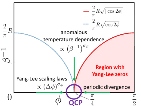
Figure 1: Phase diagram of the Yang-Lee quantum critical system. The quantum critical point (QCP) is located at $\phi=\pi/4$ and $\beta^{-1}=0$. In the $\mathcal{PT}$-unbroken phase (i.e., $|\phi|<\pi/4$), the $\Delta\phi$ dependences of physical quantities reproduce the conventional scaling laws for the Yang-Lee edge singularity Fisher (1980); Note (3) in two successive limits, i.e., $\beta^{-1}\to 0$ followed by $\phi\to\pi/4-0$. In the $\mathcal{PT}$-broken phase (i.e., $|\phi|>\pi/4$), physical quantities exhibit periodic divergence and the corresponding limits cannot be defined by two sequential limits of $\beta^{-1}\to 0$ followed by $\phi\to\pi/4+0$. Unconventional scaling laws for the dependence on the temperature $\beta^{-1}$ are obtained if the limit of $\beta^{-1}\to 0$ is taken after the limit of $\phi\to\pi/4$. In the $\mathcal{PT}$-unbroken phase, a crossover between the two limiting behaviors occurs near the dotted curve given by $\beta^{-1}=\quantity(2/\pi)R\sqrt{\cos 2\phi}$.

Next, we consider the $\mathcal{PT}$-broken phase (i.e., $|\phi|>\pi/4$) and evaluate the dependence of physical quantities on $\Delta\phi$ by taking the limit $\phi\to\pi/4+0$ after $\beta^{-1}\to 0$. In this phase, the magnetization is given by $m=-i\quantity(\sin\phi/\sqrt{|\cos 2\phi|})\tan(\beta R\sqrt{|\cos 2\phi|})$ and exhibits periodic divergence when the limit $\beta^{-1}\to 0$ is taken for some fixed $\phi>\pi/4$, which makes it impossible to define the above-mentioned two limits of $m$ (see Fig. 1). The condition for the divergence is given by $\beta R\sqrt{|\cos 2\phi|}=\quantity(n+1/2)\pi$ for some integer $n$, which corresponds to the zeros of $Z=2\cos(\beta R\sqrt{|\cos 2\phi|})$, i.e., the Yang-Lee zeros. Here, the real-valuedness of $\phi$ which satisfies this condition is in accordance with the Lee-Yang circle theorem Lee and Yang (1952); Note (1); Simon and Griffiths (1973); Newman (1974); Lieb and Sokal (1981). These zeros appear only in the region given by $\beta^{-1}\leq\quantity(2/\pi)R\sqrt{|\cos 2\phi|}$ (see Fig. 1). As in the case of magnetization, the two successive limits of the magnetic susceptibility and the two-time correlation function also cannot be taken because of the periodic divergence at the Yang-Lee zeros.

Finally, we consider the case in which the limit $\beta^{-1}\to 0$ is taken after $\phi\to\pi/4$. This order of the two limits leads to unconventional scaling laws that have not been discussed in classical systems. By taking the limit of $\phi\to\pi/4$, we obtain the following unconventional scaling laws Note (3):

$$m\to-\frac{i}{\sqrt{2}}\beta R,\quad\chi\to-\frac{i}{3\sqrt{2}}\quantity(\beta^{3}R^{3}+\frac{3}{2}\beta R),$$

$$G\quantity(t_{2},t_{1})\to R^{2}\quantity(\frac{1}{2}\beta^{2}-i\beta\Delta t-(\Delta t)^{2})+1,$$ (16)

from which we obtain critical exponents $-1,-3,-2$ for the dependence on the temperature $\beta^{-1}$ (see Fig. 1). In particular, the two-time correlation function behaves as $\quantity|G\quantity(t_{2},t_{1})|\propto\quantity(\Delta t)^{2}$ in the limit of $\Delta t\to\infty$, which is consistent with the anomalous divergent behavior of the spatial correlation function $G_{\rm cl}(x)\propto x^{2}$ at the critical point of the corresponding classical system Fisher (1980); Note (3). To understand the physical origin of the divergent behavior in the quantum system, we note that the factor $\cosh\quantity[(\beta-2i\Delta t)R\sqrt{\cos 2\phi}]$ in the two-time correlation function (11) becomes $\cosh\quantity[(i\beta+2\Delta t)R\sqrt{|\cos 2\phi|}]$ in the $\mathcal{PT}$-broken phase and exponentially diverges in a time scale $T\propto|\cos 2\phi|^{-1/2}$ as $\Delta t$ increases, indicating an exponential amplification in this phase Konotop et al. (2016); Feng et al. (2017); El-Ganainy et al. (2018); Miri and Alù (2019); Özdemir et al. (2019). At the critical point (i.e., $\phi=\pm\pi/4$), the time scale $T$ diverges and the divergent behavior of the two-time correlation function becomes a power law. We note that we can observe the criticality in Eq. (16) in the extended Hermitian system by examining the temperature dependence of physical quantities while fixing the parameters $r$ and $\theta$ near the critical point.

In the $\mathcal{PT}$-unbroken phase (i.e., $|\phi|<\pi/4$), a crossover between the two limiting behaviors occurs around $\beta^{-1}\simeq\quantity(2/\pi)R\sqrt{\cos 2\phi}$, where the temperature is comparable to the energy gap (see Fig. 1).

Experimental situation. —

The dynamics governed by the non-Hermitian Hamiltonian $H_{\rm PT}$ has been experimentally realized in open quantum systems Tang et al. (2016); Li et al. (2019); Xiao et al. (2019); Wu et al. (2019), and the scheme for embedding this non-Hermitian Hamiltonian in the Hermitian two-qubit system discussed in this Letter has been implemented Tang et al. (2016); Xiao et al. (2019). Among various quantum simulators, a system of trapped ions Bollinger et al. (1991); Cirac and Zoller (1995); Monroe et al. (1995); Turchette et al. (1998); Sackett et al. (2000); Benhelm et al. (2008); Myerson et al. (2008); Kim et al. (2009, 2010); Brown et al. (2011); Lanyon et al. (2011); Islam et al. (2011); Britton et al. (2012); Islam et al. (2013); Jurcevic et al. (2014); Richerme et al. (2014); Smith et al. (2016); Bohnet et al. (2016); Zhang et al. (2017); Wang et al. (2017); Bruzewicz et al. (2019) is an ideal one to explore the long-time dynamics at finite temperatures due to a long coherence time Bollinger et al. (1991); Wang et al. (2017).

The Yang-Lee edge singularity in the magnetization $m$ of the system can be found from Eq. (6) through measurement of Note (3)

$$m =\frac{\Tr_{\rm tot}\!\quantity[\quantity(\sigma_{\rm A}^{x}\otimes\sigma^{z})\tilde{\rho}_{\rm TFI}]-i\Tr_{\rm tot}\!\quantity[\quantity(\sigma_{\rm A}^{z}\otimes\sigma^{z})\tilde{\rho}_{\rm TFI}]}{\Tr_{\rm tot}\!\quantity[\quantity(\sigma_{\rm A}^{x}\otimes I)\tilde{\rho}_{\rm TFI}]-i\Tr_{\rm tot}\!\quantity[\quantity(\sigma_{\rm A}^{z}\otimes I)\tilde{\rho}_{\rm TFI}]},$$ (17)

where $\tilde{\rho}_{\rm TFI}=P^{\prime}_{\rm tot}\rho_{\rm TFI}P^{\prime}_{\rm tot}$. Here $\rho_{\rm TFI}=e^{-\beta H_{\rm TFI}}/\Tr_{\rm tot}[e^{-\beta H_{\rm TFI}}]$ is a thermal equilibrium state of the total system for the Ising Hamiltonian with a transverse field $H_{\rm TFI}=r\sin\theta~{}I_{\rm A}\otimes\sigma^{x}+r\cos\theta~{}\sigma_{\rm A}^{z}\otimes\sigma^{z}$, which is related to $H_{\rm tot}$ as $H_{\rm tot}=e^{\frac{\pi}{4}i\sigma_{\rm A}^{x}}H_{\rm TFI}e^{-\frac{\pi}{4}i\sigma_{\rm A}^{x}}$. The transverse-field Ising Hamiotonian has been implemented in trapped ions Kim et al. (2009, 2010); Lanyon et al. (2011); Islam et al. (2011); Britton et al. (2012); Islam et al. (2013); Jurcevic et al. (2014); Richerme et al. (2014); Smith et al. (2016); Bohnet et al. (2016); Zhang et al. (2017), superconducting-circuit QED systems Tian (2010); Viehmann et al. (2013a, b); Zhang et al. (2014); Harris et al. (2018); King et al. (2018) and Rydberg atoms Schauß et al. (2012); Zeiher et al. (2015); Schauß et al. (2015); Labuhn et al. (2016); Bernien et al. (2017); Lienhard et al. (2018); Guardado-Sanchez et al. (2018); Browaeys and Lahaye (2020). The projection operator $P^{\prime}_{\rm tot}$ is given by $e^{-\frac{\pi}{4}i\sigma_{\rm A}^{x}}P_{\rm tot}^{\rm PT}e^{\frac{\pi}{4}i\sigma_{\rm A}^{x}}=\frac{1}{2}\quantity(I+\tilde{H}^{\prime})$, where $\tilde{H}^{\prime}:=\sin\theta~{}\sigma_{\rm A}^{x}\otimes I-\cos\theta~{}\sigma_{\rm A}^{y}\otimes\sigma^{y}$, and it can be implemented by projection onto the eigenspace of $\tilde{H}^{\prime}$ with eigenvalue $+1$ using, for example, the scheme proposed in Ref. Yang et al. (2020), in which the center of mass of trapped ions is coupled to atomic states and plays a role of the meter in an indirect measurement of the Hamiltonian.

The two-time correlation function $G\quantity(\sigma^{z}(t_{2}),\sigma^{z}(t_{1}))$ can be measured in a similar manner. Specifically, from Eq. (7), $\expectationvalue{\sigma^{z}(t_{2})\sigma^{z}(t_{1})}_{\rm PT}$ is obtained as the ratio between the following quantities Note (3):

$$\expectationvalue{\quantity[\quantity(\sigma_{\rm A}^{x}-i\sigma_{\rm A}^{z})\otimes O_{\rm S}]_{\rm TFI}(\Delta t)P^{\prime}_{\rm tot}\quantity[\quantity(\sigma_{\rm A}^{x}-i\sigma_{\rm A}^{z})\otimes O_{\rm S}]P^{\prime}_{\rm tot}}_{\rm TFI},$$ (18)

where $O_{\rm S}=\sigma^{z}\,(I)$ for the numerator (denominator), $\expectationvalue{O}_{\rm TFI}=\Tr_{\rm tot}\quantity[O\rho_{\rm TFI}]$, and $\quantity[O]_{\rm TFI}(t)=e^{itH_{\rm TFI}}Oe^{-itH_{\rm TFI}}$. The quantity in Eq. (18) is obtained as a linear combination of quantities such as $\expectationvalue{\quantity[O^{\prime}_{\rm A}\otimes O_{\rm S}]_{\rm TFI}(\Delta t)P^{\prime}_{\rm tot}\quantity[O_{\rm A}\otimes O_{\rm S}]P^{\prime}_{\rm tot}}_{\rm TFI}$ ($O_{\rm A},O^{\prime}_{\rm A}\in\{\sigma_{\rm A}^{x},\sigma_{\rm A}^{z}\}$), and this quantity can be evaluated using the polarization identity Gardiner and Zoller (2004):

$$A^{{\dagger}}MB=\frac{1}{4}\left[(A+B)^{{\dagger}}M(A+B)-(A-B)^{{\dagger}}M(A-B)\right.$$

$$\left.-i(A+iB)^{{\dagger}}M(A+iB)+i(A-iB)^{{\dagger}}M(A-iB)\right].$$ (19)

Indeed, we can apply this identity to the quantity in $\expectationvalue{\cdots}_{\rm TFI}$ with $A=I$, $M=\quantity[O^{\prime}_{\rm A}\otimes O_{\rm S}]_{\rm TFI}(\Delta t)$, and $B=P^{\prime}_{\rm tot}\quantity[O_{\rm A}\otimes O_{\rm S}]P^{\prime}_{\rm tot}$. Then the desired quantity is evaluated as a linear combination of quantities such as $\expectationvalue{(A+B)^{{\dagger}}M(A+B)}_{\rm TFI}$, which is obtained by first applying $A+B=I+P^{\prime}_{\rm tot}\quantity[O_{\rm A}\otimes O_{\rm S}]P^{\prime}_{\rm tot}$ to the thermal equilibrium state $\rho_{\rm TFI}$ and then measuring $O^{\prime}_{\rm A}\otimes O_{\rm S}$ after a time interval $\Delta t$.

Summary and future perspectives. —

We have identified a quantum system which exhibits the Yang-Lee edge singularity on the basis of the quantum-classical correspondence and discussed its realization in an open quantum system. Specifically, we have embedded the non-Hermitian quantum system in an extended Hermitian system by introducing an ancilla, and found that the physical origin of the singularity lies in the facts that the physical quantity to be evaluated is the expectation value conditioned on the measurement outcome of the ancilla and that the probability of the successful postselection of events almost vanishes in the vicinity of the critical point. Moreover, we have found unconventional scaling laws for finite-temperature dynamics, which are unique to quantum critical phenomena Sachdev (2001). We have shown that an expectation value over the canonical ensemble with respect to a non-Hermitian Hamiltonian corresponds to that for an extended Hermitian system with the projection onto specific matrix elements of the reduced density matrix of the ancilla (see Eq. (6)). It is worthwhile to investigate the generality of this correspondence.

The Yang-Lee edge singularity is a prototypical example of nonunitary critical phenomena involving anomalous scaling laws that cannot be found in unitary critical systems. We hope that this work stimulates further investigation on nonunitary critical phenomena in open quantum systems for higher-dimensional systems and other universality classes.

We are grateful to Kohei Kawabata, Hosho Katsura, and Takashi Mori for fruitful discussions. This work was supported by KAKENHI Grant No. JP22H01152 from the Japan Society for the Promotion of Science (JSPS). N. M. was supported by the JSPS through Program for Leading Graduate Schools (MERIT). N. M. and M. N. were supported by JSPS KAKENHI Grants No. JP21J11280 and No. JP20K14383.

Supplemental Material for
“Embedding the Yang-Lee Quantum Criticality in Open Quantum Systems”

I Yang-Lee edge singularity in the classical one-dimensional Ising model

We briefly review the Yang-Lee edge singularity Kortman and Griffiths (1971); Fisher (1978); Kurtze and Fisher (1979); Fisher (1980); Cardy (1985); Cardy and Mussardo (1989); Zamolodchikov (1991) in the classical one-dimensional ferromagnetic Ising model Fisher (1980):

$$H=-J\sum_{j}\sigma_{j}\sigma_{j+1}-h\sum_{j}\sigma_{j},$$ (S1)

where $J$ is positive and $h$ is complex in general. The corresponding transfer matrix is given by

and their eigenvalues are given by

$$\lambda_{\pm}=e^{\beta J}\cosh{\beta h}\pm\sqrt{e^{2\beta J}\sinh^{2}{\beta h}+e^{-2\beta J}}.$$ (S2)

Under the periodic boundary condition, the partition function is represented as $Z=\Tr[T^{N}]$, where $N$ is the number of sites. In the thermodynamic limit $N\to\infty$, the free energy density is given by

$$f=-\frac{1}{\beta N}\ln\lambda_{+}^{N}=-\frac{1}{\beta}\ln(e^{\beta J}\cosh{\beta h}+\sqrt{e^{2\beta J}\sinh^{2}{\beta h}+e^{-2\beta J}}),$$ (S3)

and the correlation length is given by

$$\xi=\frac{1}{\ln\lambda_{+}-\ln\lambda_{-}}.$$ (S4)

From Eq. (S4), we find that the Yang-Lee edge singularity exhibits the diverging correlation length when the magnetic field satisfies the following condition:

$$e^{2\beta J}\sinh^{2}{\beta h}+e^{-2\beta J}=0,$$ (S5)

and hence the critical magnetic field is pure imaginary:

$$h_{c}=\pm i\beta^{-1}\sin^{-1}(e^{-2\beta J}),$$ (S6)

which is in accordance with the Lee-Yang circle theorem Lee and Yang (1952); Simon and Griffiths (1973); Newman (1974); Lieb and Sokal (1981).

The Yang-Lee edge singularity involves anomalous scaling laws with no counterparts in unitary critical phenomena. The magnetization density is obtained as $m=-\partial_{h}f$, which scales in the vicinity of the critical point as

$$m=\frac{\sinh{\beta h}}{\sqrt{\sinh^{2}{\beta h}+e^{-4\beta J}}}=\frac{\sinh{\beta h}}{\sqrt{C\Delta{h}+o(\Delta{h})}}\propto\Delta h^{\sigma},\quad\sigma=-\frac{1}{2},$$ (S7)

where $\Delta h:=h-h_{c}$, and $C$ is some nonuniversal constant. By differentiating the magnetization density with respect to the magnetic field, we obtain the scaling law for the magnetic susceptibility:

$$\chi=\derivative{m}{h}=\frac{\beta\,e^{-4\beta J}\cosh(\beta h)}{\quantity(\sinh^{2}{\beta h}+e^{-4\beta J})^{3/2}}\propto\frac{1}{\Delta h^{\gamma}},\quad\gamma=1-\sigma=\frac{3}{2}.$$ (S8)

Correlation functions also exhibit anomalous scaling laws. From the expression in Eq. (S4), the correlation length scales near the critical point as

$$\xi^{-1}\simeq 2e^{-\beta J}(\cosh{\beta h})^{-1}\sqrt{e^{2\beta J}\sinh^{2}{\beta h}+e^{-2\beta J}}=2(\cosh{\beta h})^{-1}\sqrt{C\Delta{h}+o\quantity(\Delta{h})}\propto\Delta{h}^{1/2}.$$ (S9)

Hence we obtain the critical exponent as follows:

$$\xi\propto\frac{1}{\Delta h^{\nu}},\hskip 28.45274pt\nu=\frac{1}{2}.$$ (S10)

Finally, the correlation function $G_{\rm cl}(x)$ at spatial distance $x$ scales as

$$G_{\rm cl}(x)=\frac{1}{1+e^{4\beta J}\sinh^{2}(\beta h)}\quantity(\frac{\lambda_{-}}{\lambda_{+}})^{x}\propto\frac{1}{\Delta h}e^{-x/\xi}\propto\frac{e^{-x/\xi}}{\quantity(x/\xi)^{2}}x^{-\quantity(d-2+\eta)},$$ (S11)

where $d=1$ and $\eta=-1$.

II quantum-classical correspondence

In this section, we discuss the quantum-classical correspondence Suzuki (1976); Kogut (1979) between the classical one-dimensional ferromagnetic Ising model $H=-J\sum_{j}\sigma_{j}\sigma_{j+1}-ih_{\rm cl}\sum_{j}\sigma_{j}$ ($J>0,h_{\rm cl}\in\mathbb{R}$) and a parity-time ($\mathcal{PT}$) symmetric non-Hermitian Hamiltonian Bender and Boettcher (1998); Bender et al. (2002); Bender (2007) $H_{\rm Q}=-\quantity(h_{x}\sigma^{x}+ih_{z}\sigma^{z})$ with real parameters $h_{x}$ and $h_{z}$, which is summarized as shown in Table S1.

	quantum system	classical system	upper bound or leading-order term of the error between the two systems
$\beta=\beta_{0}n_{\rm temp}$	inverse temperature	system size	—
$\beta_{0}/n_{\rm div}$	segment width of inverse temperature	lattice constant	—
$N=n_{\rm temp}n_{\rm div}$	number of segments in inverse temperature	number of sites	—
$n_{\rm temp}\to\infty$	zero-temperature limit	thermodynamic limit	—
$n_{\rm div}\to\infty$	continuum limit for imaginary time	continuum limit for real space	—
partition function	$\Tr[e^{\beta\quantity(h_{x}\sigma^{x}+ih_{z}\sigma^{z})}]$	$A^{\!N}\sum_{\{\!\sigma_{k}\!\}}e^{\sum_{k}\quantity(\beta_{\rm cl}J\sigma_{k+1}\sigma_{k}+i\beta_{\rm cl}h_{\rm cl}\sigma_{k})}$	$\quantity|Z_{\rm Q}-Z_{\rm cl}|\leq$ $\frac{2n_{\rm temp}\beta_{0}^{3}(|h_{x}|+|h_{z}|)^{3}}{3n_{\rm div}^{2}}e^{n_{\rm temp}\beta_{0}(|h_{x}|+|h_{z}|)}$
free-energy density	$-\frac{1}{\beta_{0}n_{\rm temp}}$ $\ln Z_{\rm Q}$	$-\frac{1}{\beta_{\rm cl}n_{\rm div}n_{\rm temp}}$ $\ln Z_{\rm cl}$	$\quantity|f_{\rm Q}-f_{\rm cl}|\leq$ $\frac{2\beta_{0}^{2}(|h_{x}|+|h_{z}|)^{3}}{3n_{\rm div}^{2}Z_{\rm cl}}$ $e^{n_{\rm temp}\beta_{0}(|h_{x}|+|h_{z}|)}$
magnetization in the limit $n_{\rm temp}\to\infty$	$-i$ $\frac{\sin\phi}{\sqrt{\cos 2\phi}}$	$i$$\frac{\sin(\beta_{\rm cl}h_{\rm cl})}{\sqrt{\exp(-4\beta_{\rm cl}J)-\sin^{2}(\beta_{\rm cl}h_{\rm cl})}}$	$\frac{1}{24}\frac{\cos^{2}\phi}{(\cos 2\phi)^{3/2}}$ $\quantity|\sin\phi-3\sin 3\phi|$$\quantity(\!\frac{\beta_{0}R}{n_{\rm div}}\!)^{\!\!2}$$+\,\mathcal{O}\quantity(n_{\rm div}^{\!-4})$
magnetic susceptibility in the limit $n_{\rm temp}\to\infty$	$-i$$\frac{\cos^{3}\phi}{(\cos 2\phi)^{3/2}}$	$i\beta_{\rm cl}$ $\frac{\exp(-4\beta_{\rm cl}J)\cos(\beta_{\rm cl}h_{\rm cl})}{\quantity[\exp(-4\beta_{\rm cl}J)-\sin^{2}(\beta_{\rm cl}h_{\rm cl})]^{3/2}}$	$\frac{1}{16}\frac{\cos^{3}\phi}{(\cos 2\phi)^{5/2}}$ $\left|3\!+\!12\cos 2\phi\!+\!\cos 4\phi\right|$$\quantity(\!\frac{\beta_{0}R}{n_{\rm div}}\!)^{\!\!2}$$+\,\mathcal{O}\quantity(n_{\rm div}^{\!-4})$
correlation function in the limit $n_{\rm temp}\to\infty$	$\frac{\cos^{2}\!\phi}{\cos 2\phi}$ $e^{-2R\Delta\tau\sqrt{\cos 2\phi}}$	$\frac{1}{1-e^{4\beta_{\rm cl}J}\sin^{2}(\beta_{\rm cl}h_{\rm cl})}$ $\times\!\quantity[\!\frac{\cos(\beta_{\rm cl}h_{\rm cl})-\sqrt{e^{-4\beta_{\rm cl}J}-\sin^{2}(\beta_{\rm cl}h_{\rm cl})}}{\cos(\beta_{\rm cl}h_{\rm cl})+\sqrt{e^{-4\beta_{\rm cl}J}-\sin^{2}(\beta_{\rm cl}h_{\rm cl})}}]^{\!x}$	$\frac{\tan^{2}2\phi}{24}$ $\left|1\!+\!2R\Delta\tau(\cos^{2}\!\phi)\sqrt{\cos 2\phi}+3\cos 2\phi\right|$ $\hskip 42.67912pt\times\,e^{-2R\Delta\tau\sqrt{\cos 2\phi}}$ $\quantity(\!\frac{\beta_{0}R}{n_{\rm div}}\!)^{\!\!2}$ $+\,\mathcal{O}\quantity(n_{\rm div}^{\!-4})$

Table S1: Quantum-classical correspondence between a quantum system with a parity-time symmetric non-Hermitian Hamiltonian and a classical one-dimensional ferromagnetic Ising model. Parameters in the two systems are related via $\beta_{\rm cl}J=-\frac{1}{2}\ln\quantity[\tanh(\beta_{0}h_{x}/n_{\rm div})]$ and $\beta_{\rm cl}h_{\rm cl}=\beta_{0}h_{z}/n_{\rm div}$.

This correspondence is based on the equivalence of the partition functions. The partition function for $H_{\rm Q}$ is given by

$$Z_{\rm Q}=\Tr\quantity[e^{-\beta H_{\rm Q}}]=\sum_{\sigma_{0}=\pm 1}\expectationvalue{e^{-(\beta_{0}n_{\rm temp})H_{\rm Q}}}{\sigma_{0}},$$ (S53)

where $\ket{\sigma_{0}}$ is the eigenstate of $\sigma^{z}$ with the eigenvalue $\sigma_{0}\in\{+1,-1\}$, and the inverse temperature $\beta$ is given by $\beta=\beta_{0}n_{\rm temp}$ with an integer $n_{\rm temp}$ and a fixed value $\beta_{0}$. We employ a path-integral representation of this quantity Feynman (1948, 1949) by dividing each segment $\beta_{0}$ into $n_{\rm div}$ subsegments, resulting in $N=n_{\rm temp}n_{\rm div}$ subsegments with a width $\beta_{0}/n_{\rm div}$ in total. By inserting a complete set between each successive pair of subsegments, we obtain

$$Z_{\rm Q} =\sum_{\sigma_{0}=\pm 1}\expectationvalue{\quantity[\quantity(\exp(\frac{\beta_{0}h_{x}}{n_{\rm div}}\sigma^{x})\exp(i\frac{\beta_{0}h_{z}}{n_{\rm div}}\sigma^{z}))^{n_{\rm temp}n_{\rm div}}+E_{n_{\rm div},n_{\rm temp}}]}{\sigma_{0}}$$

$$=\sum_{\sigma_{0}}\cdots\sum_{\sigma_{N-1}}\prod_{k=0}^{N-1}\matrixelement{\sigma_{k+1}}{\exp(\frac{\beta_{0}h_{x}}{n_{\rm div}}\sigma^{x})\exp(i\frac{\beta_{0}h_{z}}{n_{\rm div}}\sigma^{z})}{\sigma_{k}}+\Tr[E_{n_{\rm div},n_{\rm temp}}]$$

$$=\sum_{\sigma_{0}}\cdots\sum_{\sigma_{N-1}}A^{N}\exp[\sum_{k=0}^{N-1}\quantity(\beta_{\rm cl}J\sigma_{k+1}\sigma_{k}+i\beta_{\rm cl}h_{\rm cl}\sigma_{k})]+\Tr[E_{n_{\rm div},n_{\rm temp}}],$$ (S54)

where $\sigma_{N}=\sigma_{0}$, and the coefficients are given by

$$A:=\sqrt{\cosh(\frac{\beta_{0}h_{x}}{n_{\rm div}})\sinh(\frac{\beta_{0}h_{x}}{n_{\rm div}})},\quad\quad\beta_{\rm cl}J:=-\frac{1}{2}\ln\quantity[\tanh(\frac{\beta_{0}h_{x}}{n_{\rm div}})],\quad\quad\beta_{\rm cl}h_{\rm cl}:=\frac{\beta_{0}h_{z}}{n_{\rm div}}.$$ (S55)

Here, we have used the following evaluation of a matrix element:

$$\matrixelement{\sigma_{k+1}}{\exp(\frac{\beta_{0}h_{x}}{n_{\rm div}}\sigma^{x})\exp(i\frac{\beta_{0}h_{z}}{n_{\rm div}}\sigma^{z})}{\sigma_{k}} =\matrixelement{\sigma_{k+1}}{\quantity[\cosh(\frac{\beta_{0}h_{x}}{n_{\rm div}})+\sinh(\frac{\beta_{0}h_{x}}{n_{\rm div}})\sigma^{x}]}{\sigma_{k}}\exp(i\frac{\beta_{0}h_{z}}{n_{\rm div}}\sigma_{k})$$

$$=\quantity[\cosh(\frac{\beta_{0}h_{x}}{n_{\rm div}})\delta_{\sigma_{k+1},\sigma_{k}}+\sinh(\frac{\beta_{0}h_{x}}{n_{\rm div}})\quantity(1-\delta_{\sigma_{k+1},\sigma_{k}})]\exp(i\frac{\beta_{0}h_{z}}{n_{\rm div}}\sigma_{k})$$

$$=A\exp(\beta_{\rm cl}J\sigma_{k+1}\sigma_{k})\exp(i\frac{\beta_{0}h_{z}}{n_{\rm div}}\sigma_{k}).$$ (S56)

The right-hand side of Eq. (S54) gives the partition function $Z_{\rm cl}$ for the classical one-dimensional ferromagnetic Ising model, which shows the desired correspondence for the partition functions. Here, the error between the quantum and classical systems is bounded from above as Suzuki (1985a)

$$\quantity|Z_{\rm Q}-Z_{\rm cl}|=\quantity|\,\Tr[E_{n_{\rm div},n_{\rm temp}}]\,|\leq\frac{2n_{\rm temp}\beta_{0}^{3}(|h_{x}|+|h_{z}|)^{3}}{3n_{\rm div}^{2}}e^{n_{\rm temp}\beta_{0}(|h_{x}|+|h_{z}|)},$$ (S57)

which is vanishingly small in the continuum limit $n_{\rm div}\rightarrow\infty$. As a corollary of this bound, we also evaluate the error of the free-energy density as

$$|f_{\rm Q}-f_{\rm cl}| =\quantity|\quantity(-\frac{1}{\beta_{0}n_{\rm temp}}\ln Z_{\rm Q})-\quantity(-\frac{1}{\beta_{\rm cl}n_{\rm div}n_{\rm temp}}\ln Z_{\rm cl})|=\frac{1}{\beta_{0}n_{\rm temp}}\ln(1+\frac{\quantity|\Tr[E_{n_{\rm div},n_{\rm temp}}]|}{Z_{\rm cl}})$$

$$\leq\frac{1}{\beta_{0}n_{\rm temp}}\frac{\quantity|\Tr[E_{n_{\rm div},n_{\rm temp}}]|}{Z_{\rm cl}}\leq\frac{2\beta_{0}^{2}(|h_{x}|+|h_{z}|)^{3}}{3n_{\rm div}^{2}Z_{\rm cl}}e^{n_{\rm temp}\beta_{0}(|h_{x}|+|h_{z}|)},$$ (S58)

where we have set the inverse temperature of the classical system as $\beta_{\rm cl}=\beta_{0}/n_{\rm div}$.

Next, we evaluate the error between physical observables of the quantum and classical systems. In the classical system, magnetization density, magnetic susceptibility and spatial correlation function are given in the thermodynamic limit $n_{\rm temp}\rightarrow\infty$ by (see Eqs. (S7), (S8), (S11))

$$m_{\rm cl} \to i\frac{\sin(\beta_{\rm cl}h_{\rm cl})}{\sqrt{\exp(-4\beta_{\rm cl}J)-\sin^{2}(\beta_{\rm cl}h_{\rm cl})}},\hskip 28.45274pt\chi_{\rm cl}\to i\beta_{\rm cl}\frac{\exp(-4\beta_{\rm cl}J)\cos(\beta_{\rm cl}h_{\rm cl})}{\quantity[\exp(-4\beta_{\rm cl}J)-\sin^{2}(\beta_{\rm cl}h_{\rm cl})]^{3/2}},$$

$$G_{\rm cl}(x) \to\frac{1}{1-e^{4\beta_{\rm cl}J}\sin^{2}(\beta_{\rm cl}h_{\rm cl})}\quantity(\frac{\cos(\beta_{\rm cl}h_{\rm cl})-\sqrt{\exp(-4\beta_{\rm cl}J)-\sin^{2}(\beta_{\rm cl}h_{\rm cl})}}{\cos(\beta_{\rm cl}h_{\rm cl})+\sqrt{\exp(-4\beta_{\rm cl}J)-\sin^{2}(\beta_{\rm cl}h_{\rm cl})}})^{\!x}.$$ (S59)

On the other hand, in the quantum system, where the same limit $n_{\rm temp}\rightarrow\infty$ represents the zero-temperature limit, the corresponding observables are given by (see Eqs. (S88), (S89), (S90) )

$$m_{\rm Q}\to-i\frac{\sin\phi}{\sqrt{\cos 2\phi}},\hskip 28.45274pt\chi_{\rm Q}\to-i\frac{\cos^{3}\phi}{\quantity(\cos 2\phi)^{3/2}},\hskip 28.45274ptG_{\rm Q}\quantity(\Delta\tau)\to\frac{\cos^{2}\phi}{\cos 2\phi}\,\exp\!\quantity(-2R\Delta\tau\sqrt{\cos 2\phi}),$$ (S60)

where $\Delta\tau=(\beta_{0}/n_{\rm div})x$ and the parametrization in the main text is reproduced by the relation $h_{x}=-R\cos\phi$ and $h_{z}=-R\sin\phi$. Imposing the relationship in Eq. (S55), we evaluate the error in each observable between the quantum and classical systems in the same limit $n_{\rm temp}\to\infty$:

$$m_{\rm Q}-m_{\rm cl}\to-\frac{i}{24}\frac{\cos^{2}\phi}{(\cos 2\phi)^{3/2}}\quantity[\sin\phi-3\sin(3\phi)]\quantity(\frac{\beta_{0}R}{n_{\rm div}})^{2}+\mathcal{O}\quantity(n_{\rm div}^{-4}),$$

$$\chi_{\rm Q}-\quantity(-\frac{\beta_{\rm cl}n_{\rm div}}{\beta_{0}R\cos\phi})^{-1}\chi_{\rm cl}\to\frac{i}{16}\frac{\cos^{3}\phi}{(\cos 2\phi)^{5/2}}\quantity[3+12\cos(2\phi)+\cos(4\phi)]\quantity(\frac{\beta_{0}R}{n_{\rm div}})^{2}+\mathcal{O}\quantity(n_{\rm div}^{-4}),$$

$$G_{\rm Q}(\Delta\tau)-G_{\rm cl}(x)\to-\frac{\tan^{2}(2\phi)}{24}\quantity[1+2R\Delta{\color[rgb]{0,0,0}\tau}(\cos^{2}\!\phi)\sqrt{\cos(2\phi)}+3\cos(2\phi)]{\color[rgb]{0,0,0}e^{-2R\Delta\tau\sqrt{\cos 2\phi}}}\quantity(\frac{\beta_{0}R}{n_{\rm div}})^{\!2}+\mathcal{O}\quantity(n_{\rm div}^{-4}),$$ (S61)

where we have rescaled the magnetic susceptibility for the classical system taking the difference in the magnetic field between the two systems into account. Here, the scaling $\mathcal{O}\quantity(n_{\rm div}^{-2})$ of the leading term in the errors is consistent with the general argument given in Refs. Suzuki (1985a, b).

Then, we consider how finely we should divide the inverse temperature in the quantum system to obtain the quantum-classical correspondence with an error smaller than a given precision $\epsilon$. We argue that the integer $n_{\rm div}$ should be chosen large enough so as to satisfy

$$\frac{n_{\rm div}}{\beta_{0}R}>\frac{1}{\sqrt{\epsilon}\,\quantity(\cos 2\phi)^{5/4}}.$$ (S62)

Under this condition, (i) higher-order terms in $n_{\rm div}^{-1}$ in the error of observables can be relatively neglected while (ii) the leading term is bounded by $\epsilon$ from above. To demonstrate the argument (i), we consider the expansion of the error in magnetization density in the limit of $n_{\rm temp}\rightarrow\infty$:

$$m_{\rm Q}-m_{\rm cl}\to -\frac{i}{24\sqrt{2}}\frac{1}{(\cos 2\phi)^{3/2}}\quantity(\frac{\beta_{0}R}{n_{\rm div}})^{2}+\frac{i}{384\sqrt{2}}\frac{1}{(\cos 2\phi)^{5/2}}\quantity(\frac{\beta_{0}R}{n_{\rm div}})^{4}+i\frac{5}{27648\sqrt{2}}\frac{1}{(\cos 2\phi)^{7/2}}\quantity(\frac{\beta_{0}R}{n_{\rm div}})^{6}+\cdots.$$ (S63)

Here, if $n_{\rm div}$ is large enough to satisfy the condition in Eq. (S62), higher-order terms can be relatively neglected since we have

$$\frac{1}{\cos 2\phi}\quantity(\frac{\beta_{0}R}{n_{\rm div}})^{2}<\epsilon\,(\cos 2\phi)^{3/2}\ll 1.$$ (S64)

The above argument holds also for the magnetic susceptibility and the correlation function. Furthermore, the argument (ii) is demonstrated as shown in the following:

$$\frac{\Delta m}{\epsilon} =\frac{1}{\epsilon}\quantity[\frac{1}{24\sqrt{2}}\frac{1}{(\cos 2\phi)^{3/2}}\quantity(\frac{\beta_{0}R}{n_{\rm div}})^{2}]<\frac{\cos 2\phi}{24\sqrt{2}}<1,$$

$$\frac{\Delta\chi}{\epsilon} =\frac{1}{\epsilon}\quantity[\frac{1}{16\sqrt{2}}\frac{1}{(\cos 2\phi)^{5/2}}\quantity(\frac{\beta_{0}R}{n_{\rm div}})^{2}]<\frac{1}{16\sqrt{2}}<1,$$

$$\frac{\Delta G}{\epsilon} =\frac{1}{\epsilon}\quantity[\frac{1}{24}\frac{1}{\cos^{2}(2\phi)}\quantity(\frac{\beta_{0}R}{n_{\rm div}})^{2}]<\frac{\sqrt{\cos 2\phi}}{24}<1,$$ (S65)

where $\Delta m$, $\Delta\chi$, and $\Delta G$ denote the leading terms of the error for magnetization density, magnetic susceptibility, and correlation function, respectively.

III Derivation of the results for the extended Hermitian system

In this section, we discuss how to obtain physical quantities for the canonical ensemble of $H_{\rm PT}$ from the extended Hermitian system. First we consider the dynamics of the total system generated by $H_{\rm tot}=r\sin\theta~{}I_{\rm A}\otimes\sigma^{x}+r\cos\theta~{}\sigma_{\rm A}^{y}\otimes\sigma^{z}$ in the following two-dimensional subspace of $\mathcal{H}_{\rm tot}$:

$$\mathcal{H}_{\rm tot}^{\rm PT}=\{\ket{\psi}_{\rm tot}^{\rm PT}=\ket{\uparrow}_{\rm A}\otimes\ket{\psi}+\ket{\downarrow}_{\rm A}\otimes\quantity(\eta\ket{\psi})\,|\,\ket{\psi}\in\mathcal{H}_{\rm S}\},$$ (S66)

which is the eigenspace of the conserved quantity $\tilde{H}$ with eigenvalue $+1$. The action of $H_{\rm tot}$ is described by

$$H_{\rm tot}\ket{\psi}_{\rm tot}^{\rm PT} =\ket{\uparrow}_{\rm A}\otimes\quantity(r\sin\theta~{}\sigma^{x}-ir\cos\theta~{}\sigma^{z}\eta)\ket{\psi}+\ket{\downarrow}_{\rm A}\otimes\quantity(r\sin\theta~{}\sigma^{x}+ir\cos\theta~{}\sigma^{z}\eta^{-1})\quantity(\eta\ket{\psi})$$ (S67)

$$=\ket{\uparrow}_{\rm A}\otimes\frac{r}{\sin\theta}\quantity(\sigma^{x}-i\cos\theta~{}\sigma^{z})\ket{\psi}+\ket{\downarrow}_{\rm A}\otimes\frac{r}{\sin\theta}\quantity(\sigma^{x}+i\cos\theta~{}\sigma^{z})\quantity(\eta\ket{\psi}),$$ (S68)

which can be rewritten as

$$H_{\rm tot}\ket{\psi}_{\rm tot}^{\rm PT} =\ket{\uparrow}_{\rm A}\otimes H_{\rm PT}\ket{\psi}+\ket{\downarrow}_{\rm A}\otimes H^{{\dagger}}_{\rm PT}\quantity(\eta\ket{\psi}).$$ (S69)

Here, the non-Hermitian Hamiltonian $H_{\rm PT}$ is given by $H_{\rm PT}=R(\cos\phi)\sigma^{x}+iR(\sin\phi)\sigma^{z}$ with the parameters $R=r\sqrt{1+\cos^{2}\theta}/\sin\theta$ and $\phi=-\arctan(\cos\theta)$. This action of $H_{\rm tot}$ yields

$$e^{-itH_{\rm tot}}\ket{\psi}_{\rm tot}^{\rm PT} =\ket{\uparrow}_{\rm A}\otimes e^{-itH_{\rm PT}}\ket{\psi}+\ket{\downarrow}_{\rm A}\otimes\eta e^{-itH_{\rm PT}}\ket{\psi}.$$ (S70)

On the basis of the above result, the partition function for the system qubit with $H_{\rm PT}$ is obtained from the partition function for the total system with $H_{\rm tot}$ under the restriction of the Hilbert space to $\mathcal{H}_{\rm tot}^{\rm PT}$:

$$\Tr_{\rm tot}\quantity[P_{\rm tot}^{\rm PT}e^{-\beta H_{\rm tot}}]=\Tr_{\rm S}\quantity[e^{-\beta H_{\rm PT}}]=Z.$$ (S71)

To show this equation, we note that the projection operator can be written as

$$P_{\rm tot}^{\rm PT}=\frac{\sin\theta}{2}\sum_{\{\ket{\sigma}\}}\ket{\sigma}_{\rm tot}^{\rm PT}\ {}_{\rm tot}^{\rm PT}\bra{\eta^{-1}\sigma},$$ (S72)

where $\{\ket{\sigma}\}$ is an orthonormal basis of $\mathcal{H}_{\rm S}$ and satisfies $\braket{\sigma^{\prime}}{\sigma}=\delta_{\sigma^{\prime}\,\sigma}$. Here, the state vector $\ket{\eta^{-1}\sigma}_{\rm tot}^{\rm PT}=\ket{\uparrow}_{\rm A}\otimes\eta^{-1}\ket{\sigma}+\ket{\downarrow}_{\rm A}\otimes\ket{\sigma}\,\quantity(\in\mathcal{H}_{\rm tot}^{\rm PT})$ satisfies the following condition:

$${}_{\rm tot}^{\rm PT}\braket{\eta^{-1}\sigma^{\prime}}{\sigma}_{\rm tot}^{\rm PT}=\bra{\sigma^{\prime}}\quantity(\eta+\eta^{-1})\ket{\sigma}=\frac{2\cos\phi}{\sqrt{\cos 2\phi}}\delta_{\sigma^{\prime}\,\sigma}=\frac{2}{\sin\theta}\delta_{\sigma^{\prime}\,\sigma}.$$ (S73)

Using these expressions, the partition function is evaluated as

$$\Tr_{\rm tot}\quantity[P_{\rm tot}^{\rm PT}e^{-\beta H_{\rm tot}}] =\frac{\sin\theta}{2}\sum_{\{\ket{\sigma}\}}\ {}_{\rm tot}^{\rm PT}\bra{\eta^{-1}\sigma}e^{-\beta H_{\rm tot}}\ket{\sigma}_{\rm tot}^{\rm PT}$$

$$=\frac{\sin\theta}{2}\sum_{\{\ket{\sigma}\}}\quantity(\ {}_{\rm A}\bra{\uparrow}\otimes\bra{\sigma}\eta^{-1}+\ _{\rm A}\bra{\downarrow}\otimes\bra{\sigma})\quantity(\ket{\uparrow}_{\rm A}\otimes e^{-\beta H_{\rm PT}}\ket{\sigma}+\ket{\downarrow}_{\rm A}\otimes\eta e^{-\beta H_{\rm PT}}\ket{\sigma})$$

$$=\frac{\sin\theta}{2}\Tr_{\rm S}\quantity[\quantity(\eta+\eta^{-1})e^{-\beta H_{\rm PT}}]$$

$$=\Tr_{\rm S}\quantity[e^{-\beta H_{\rm PT}}]=Z.$$ (S74)

Then we consider the four formal expectation values $\expectationvalue{O}_{\rm tot}^{mn}$ ($m,n\in\{\uparrow,\downarrow\}$) for the canonical ensemble with respect to $H_{\rm PT}$:

$$\expectationvalue{O}_{\rm tot}^{mn}=\frac{\Tr_{\rm tot}\quantity[P_{\rm tot}^{\rm PT}\quantity(P_{\rm A}^{mn}\otimes O)e^{-\beta H_{\rm tot}}]}{\Tr_{\rm tot}\quantity[P_{\rm tot}^{\rm PT}\quantity(P_{\rm A}^{mn}\otimes I)e^{-\beta H_{\rm tot}}]}=\sum_{p}\frac{e^{-\beta E_{p}}}{Z}\frac{\matrixelement{E_{p}^{(m)}}{O}{E_{p}^{(n)}}}{\braket{E_{p}^{(m)}}{E_{p}^{(n)}}},$$ (S75)

where $\ket{E_{p}^{(m)}}:=\ket{E_{p}^{R(L)}}$ for $m=\uparrow(\downarrow)$, and $P_{\rm A}^{mn}=\ket{m}_{\rm A\ \rm A}\bra{n}$. To show this equation, we first focus on

$$\expectationvalue{O}_{\rm tot}^{\downarrow\uparrow} =\frac{\Tr_{\rm tot}\quantity[P_{\rm tot}^{\rm PT}\quantity(\sigma_{\rm A}^{-}\otimes O)e^{-\beta H_{\rm tot}}]}{\Tr_{\rm tot}\quantity[P_{\rm tot}^{\rm PT}\quantity(\sigma_{\rm A}^{-}\otimes I)e^{-\beta H_{\rm tot}}]},$$ (S76)

which exhibits the Yang-Lee edge singularity. Here, $\sigma_{\rm A}^{-}$ is defined as $\sigma_{\rm A}^{-}=(1/2)\quantity(\sigma_{\rm A}^{x}-i\sigma_{\rm A}^{y})$. The numerator of this expression is evaluated as

$$\Tr_{\rm tot}\quantity[P_{\rm tot}^{\rm PT}\quantity(\sigma_{\rm A}^{-}\otimes O)e^{-\beta H_{\rm tot}}]= \frac{\sin\theta}{2}\sum_{\{\ket{\sigma}\}}\ {}_{\rm tot}^{\rm PT}\bra{\eta^{-1}\sigma}e^{-(1-x)\beta H_{\rm tot}}\quantity(\sigma_{\rm A}^{-}\otimes O)e^{-x\beta H_{\rm tot}}\ket{\sigma}_{\rm tot}^{\rm PT}\hskip 28.45274pt\quantity(0<x<1)$$

$$= \frac{\sin\theta}{2}\sum_{\{\ket{\sigma}\}}\quantity(\ {}_{\rm A}\bra{\uparrow}\otimes\bra{\sigma}\eta^{-1}e^{-(1-x)\beta H_{\rm PT}^{{\dagger}}}+\ _{\rm A}\bra{\downarrow}\otimes\bra{\sigma}e^{-(1-x)\beta H_{\rm PT}})$$

$$\hskip 85.35826pt\times\quantity(\sigma_{\rm A}^{-}\otimes O)\quantity(\ket{\uparrow}_{\rm A}\otimes e^{-x\beta H_{\rm PT}}\ket{\sigma}+\ket{\downarrow}_{\rm A}\otimes e^{-x\beta H_{\rm PT}^{{\dagger}}}\eta\ket{\sigma})$$

$$= \frac{\sin\theta}{2}\Tr_{\rm S}[Oe^{-\beta H_{PT}}],$$ (S77)

from which we obtain the desired expression:

$$\expectationvalue{O}_{\rm tot}^{\downarrow\uparrow} =\frac{\Tr_{\rm tot}\quantity[P_{\rm tot}^{\rm PT}\quantity(\sigma_{\rm A}^{-}\otimes O)e^{-\beta H_{\rm tot}}]}{\Tr_{\rm tot}\quantity[P_{\rm tot}^{\rm PT}\quantity(\sigma_{\rm A}^{-}\otimes I)e^{-\beta H_{\rm tot}}]}=\frac{\frac{\sin\theta}{2}\Tr_{\rm S}[Oe^{-\beta H_{PT}}]}{\frac{\sin\theta}{2}Z}=\frac{\Tr_{\rm S}[Oe^{-\beta H_{PT}}]}{Z}$$

$$=\frac{1}{Z}\sum_{p}e^{-\beta E_{p}}\frac{\matrixelement{E_{p}^{L}}{O}{E_{p}^{R}}}{\braket{E_{p}^{L}}{E_{p}^{R}}}.$$ (S78)

Similar calculations yield the following results:

$$\expectationvalue{O}_{\rm tot}^{\uparrow\uparrow} =\frac{\Tr_{\rm tot}\quantity[P_{\rm tot}^{\rm PT}\quantity(P_{\rm A}^{\uparrow}\otimes O)e^{-\beta H_{\rm tot}}]}{\Tr_{\rm tot}\quantity[P_{\rm tot}^{\rm PT}\quantity(P_{\rm A}^{\uparrow}\otimes I)e^{-\beta H_{\rm tot}}]}=\frac{\frac{\sin\theta}{2}\Tr_{\rm S}\quantity[\eta^{-1}Oe^{-\beta H_{\rm PT}}]}{\frac{1}{2}Z}=\frac{1}{Z}\sum_{p}e^{-\beta E_{p}}\matrixelement{E_{p}^{R}}{O}{E_{p}^{R}},$$ (S79)

$$\expectationvalue{O}_{\rm tot}^{\downarrow\downarrow} =\frac{\Tr_{\rm tot}\quantity[P_{\rm tot}^{\rm PT}\quantity(P_{\rm A}^{\downarrow}\otimes O)e^{-\beta H_{\rm tot}}]}{\Tr_{\rm tot}\quantity[P_{\rm tot}^{\rm PT}\quantity(P_{\rm A}^{\downarrow}\otimes I)e^{-\beta H_{\rm tot}}]}=\frac{\frac{\sin\theta}{2}\Tr_{\rm S}\quantity[O\eta e^{-\beta H_{\rm PT}}]}{\frac{1}{2}Z}=\frac{1}{Z}\sum_{p}e^{-\beta E_{p}}\matrixelement{E_{p}^{L}}{O}{E_{p}^{L}},$$ (S80)

$$\expectationvalue{O}_{\rm tot}^{\uparrow\downarrow} =\frac{\Tr_{\rm tot}\quantity[P_{\rm tot}^{\rm PT}\quantity(\sigma_{\rm A}^{+}\otimes O)e^{-\beta H_{\rm tot}}]}{\Tr_{\rm tot}\quantity[P_{\rm tot}^{\rm PT}\quantity(\sigma_{\rm A}^{+}\otimes I)e^{-\beta H_{\rm tot}}]}=\frac{\frac{\sin\theta}{2}\Tr_{\rm S}[Oe^{-\beta H_{PT}^{{\dagger}}}]}{\frac{\sin\theta}{2}Z}=\frac{1}{Z}\sum_{p}e^{-\beta E_{p}}\frac{\matrixelement{E_{p}^{R}}{O}{E_{p}^{L}}}{\braket{E_{p}^{R}}{E_{p}^{L}}},$$ (S81)

from which Eq. (S75) follows. Here, $P_{\rm A}^{\uparrow},P_{\rm A}^{\downarrow},\sigma_{\rm A}^{+}$ are given by $P_{\rm A}^{\uparrow}=\ket{\uparrow}_{\rm A\ A}\bra{\uparrow}$, $P_{\rm A}^{\downarrow}=\ket{\downarrow}_{\rm A\ A}\bra{\downarrow}$, and $\sigma_{\rm A}^{+}=\ket{\uparrow}_{\rm A\ A}\bra{\downarrow}$.

Moreover, the two-time correlation function $G\quantity(O(t_{2}),O(t_{1}))=\expectationvalue{O(t_{2})O(t_{1})}_{\rm PT}-\expectationvalue{O(t_{2})}_{\rm PT}\expectationvalue{O(t_{1})}_{\rm PT}$ can be obtained in a similar manner. In particular, $\expectationvalue{O(t_{2})O(t_{1})}_{\rm PT}$ is obtained as

$$\expectationvalue{O(t_{2})O(t_{1})}_{\rm PT}=\frac{\Tr_{\rm tot}\quantity[e^{i\Delta tH_{\rm tot}}\quantity(\sigma_{\rm A}^{-}\otimes O)e^{-i\Delta tH_{\rm tot}}P_{\rm tot}^{\rm PT}\quantity(\sigma_{\rm A}^{-}\otimes O)P_{\rm tot}^{\rm PT}e^{-\beta H_{\rm tot}}]}{\Tr_{\rm tot}\quantity[e^{i\Delta tH_{\rm tot}}\quantity(\sigma_{\rm A}^{-}\otimes I)e^{-i\Delta tH_{\rm tot}}P_{\rm tot}^{\rm PT}\quantity(\sigma_{\rm A}^{-}\otimes I)P_{\rm tot}^{\rm PT}e^{-\beta H_{\rm tot}}]},$$ (S82)

where $\Delta t:=t_{2}-t_{1}$. In fact, the right-hand side is evaluated as

$$\frac{\Tr_{\rm tot}\quantity[e^{i\Delta tH_{\rm tot}}\quantity(\sigma_{\rm A}^{-}\otimes O)e^{-i\Delta tH_{\rm tot}}P_{\rm tot}^{\rm PT}\quantity(\sigma_{\rm A}^{-}\otimes O)P_{\rm tot}^{\rm PT}e^{-\beta H_{\rm tot}}]}{\Tr_{\rm tot}\quantity[e^{i\Delta tH_{\rm tot}}\quantity(\sigma_{\rm A}^{-}\otimes I)e^{-i\Delta tH_{\rm tot}}P_{\rm tot}^{\rm PT}\quantity(\sigma_{\rm A}^{-}\otimes I)P_{\rm tot}^{\rm PT}e^{-\beta H_{\rm tot}}]}$$

$$= \frac{\Tr_{\rm S}\quantity[e^{it_{2}H_{\rm PT}}\frac{\sin\theta}{2}Oe^{-i(t_{2}-t_{1})H_{\rm PT}}\frac{\sin\theta}{2}Oe^{-it_{1}H_{\rm PT}}e^{-\beta H_{\rm PT}}]}{\Tr_{\rm S}\quantity[e^{it_{2}H_{\rm PT}}\frac{\sin\theta}{2}Ie^{-i(t_{2}-t_{1})H_{\rm PT}}\frac{\sin\theta}{2}Ie^{-it_{1}H_{\rm PT}}e^{-\beta H_{\rm PT}}]}$$

$$= \frac{\Tr_{\rm S}[O(t_{2})O(t_{1})e^{-\beta H_{\rm PT}}]}{Z}=\expectationvalue{O(t_{2})O(t_{1})}_{\rm PT}.$$ (S83)

IV derivation of the scaling laws for finite-temperature quantum systems

In this section, we discuss scaling laws of physical quantities for a finite-temperature quantum system. First, we derive the magnetization, the magnetic susceptibility, and the two-time correlation function. The magnetization is calculated as

$$m:=\expectationvalue{\sigma^{z}}_{\rm PT} =\frac{\cos\phi}{\sqrt{\cos 2\phi}}\frac{e^{-\beta E_{-}}\matrixelement{E_{-}^{L}}{\sigma^{z}}{E_{-}^{R}}+e^{-\beta E_{+}}\matrixelement{E_{+}^{L}}{\sigma^{z}}{E_{+}^{R}}}{e^{-\beta E_{-}}+e^{-\beta E_{+}}}$$

$$=-i\frac{\sin\phi}{\sqrt{\cos 2\phi}}\tanh(\beta R\sqrt{\cos 2\phi}).$$ (S84)

By differentiating this with respect to $a~{}(=\tan\phi)$, we obtain the magnetic susceptibility:

$$\chi:=\derivative{m}{a}=\quantity(\cos^{2}\phi)\partialderivative{m}{\phi}=-i\frac{\cos^{3}\phi}{\quantity(\cos 2\phi)^{3/2}}\quantity[\tanh(\beta R\sqrt{\cos 2\phi})-\frac{2\beta R\quantity(\sin^{2}\phi)\sqrt{\cos 2\phi}}{\cosh^{2}\quantity(\beta R\sqrt{\cos 2\phi})}].$$ (S85)

To derive the two-time correlation function $G\quantity(\sigma^{z}(t_{2}),\sigma^{z}(t_{1}))=\expectationvalue{\sigma^{z}(t_{2})\sigma^{z}(t_{1})}_{\rm PT}-\expectationvalue{\sigma^{z}(t_{2})}_{\rm PT}\expectationvalue{\sigma^{z}(t_{1})}_{\rm PT}$, we calculate the first term on the right-hand side as follows:

$$\expectationvalue{\sigma^{z}(t_{2})\sigma^{z}(t_{1})}_{\rm PT} =\frac{1}{Z}\frac{\cos\phi}{\sqrt{\cos 2\phi}}\sum_{p\in\{+,-\}}\bra{E_{p}^{L}}e^{-(\beta-it_{2})E_{p}}\sigma^{z}\frac{\cos\phi}{\sqrt{\cos 2\phi}}\sum_{q\in\{+,-\}}\ket{E_{q}^{R}}e^{-i\quantity(t_{2}-t_{1})E_{q}}\bra{E_{q}^{L}}\sigma^{z}e^{-it_{1}E_{p}}\ket{E_{p}^{R}}$$

$$=\frac{1}{Z}\frac{\cos^{2}\phi}{\cos 2\phi}\sum_{p,q\in\{+,-\}}e^{-\beta E_{p}-i\quantity(t_{2}-t_{1})\quantity(E_{q}-E_{p})}\matrixelement{E_{p}^{L}}{\sigma^{z}}{E_{q}^{R}}\matrixelement{E_{q}^{L}}{\sigma^{z}}{E_{p}^{R}}$$

$$=\frac{1}{Z}\frac{\cos^{2}\phi}{\cos 2\phi}\sum_{p\in\{+,-\}}e^{-\beta E_{p}}\quantity(\matrixelement{E_{p}^{L}}{\sigma^{z}}{E_{p}^{R}})^{2}+\frac{1}{Z}\frac{\cos^{2}\phi}{\cos 2\phi}\sum_{p\neq q\in\{+,-\}}e^{-\beta E_{p}-i\quantity(t_{2}-t_{1})\quantity(E_{q}-E_{p})}$$

$$=-\frac{\sin^{2}\phi}{\cos 2\phi}+\frac{1}{Z}\frac{\cos^{2}\phi}{\cos 2\phi}~{}2\cosh\quantity[(\beta-2i\Delta t)R\sqrt{\cos 2\phi}]$$

$$=\frac{\cos^{2}\phi}{\cos 2\phi}\quantity(-\tan^{2}\phi+\frac{\cosh\quantity[(\beta-2i\Delta t)R\sqrt{\cos 2\phi}]}{\cosh\quantity[\beta R\sqrt{\cos 2\phi}]}),$$ (S86)

where $\Delta t:=t_{2}-t_{1}$. Combining this expression with Eq. (S84), we obtain the two-time correlation function:

$$G\quantity(\sigma^{z}(t_{2}),\sigma^{z}(t_{1})) =\expectationvalue{\sigma^{z}(t_{2})\sigma^{z}(t_{1})}_{\rm PT}-\expectationvalue{\sigma^{z}(t_{2})}_{\rm PT}\expectationvalue{\sigma^{z}(t_{1})}_{\rm PT}$$

$$=\frac{\cos^{2}\phi}{\cos 2\phi}\quantity[-\quantity(\tan^{2}\phi)\quantity(1-\tanh^{2}\quantity[\beta R\sqrt{\cos 2\phi}])+\frac{\cosh\quantity[(\beta-2i\Delta t)R\sqrt{\cos 2\phi}]}{\cosh\quantity[\beta R\sqrt{\cos 2\phi}]}].$$ (S87)

First, we consider the $\mathcal{PT}$-unbroken phase (i.e., $|\phi|<\pi/4$) and examine the dependence of physical quantities on $\Delta\phi:=\pi/4-\phi$ by taking the limit of $\phi\to\pi/4-0$ after the limit of $\beta^{-1}\to 0$. The latter corresponds to the thermodynamic limit for the classical counterpart in the quantum-classical correspondence. This order of evaluation of the two limits leads to the scaling laws in the classical system Fisher (1980). By taking the limit of $\beta^{-1}\to 0$, we obtain

$$m \to-i\frac{\sin\phi}{\sqrt{\cos 2\phi}}\propto\Delta\phi^{-\frac{1}{2}},$$ (S88)

$$\chi \to-i\frac{\cos^{3}\phi}{\quantity(\cos 2\phi)^{3/2}}\propto\Delta\phi^{-\frac{3}{2}},$$ (S89)

$$G\quantity(\sigma^{z}(t_{2}),\sigma^{z}(t_{1})) \to\frac{\cos^{2}\phi}{\cos 2\phi}\frac{\exp\quantity[(\beta-2i\Delta t)R\sqrt{\cos 2\phi}]}{\exp\quantity[\beta R\sqrt{\cos 2\phi}]}=\frac{\cos^{2}\phi}{\cos 2\phi}\exp\quantity[-2\pi i\frac{\Delta t}{\pi/\quantity(R\sqrt{\cos 2\phi})}].$$ (S90)

Here we have used the fact that hyperbolic functions behave as $\tanh(\beta R\sqrt{\cos 2\phi})\to 1$ and $\cosh\quantity[(\beta-2i\Delta t)R\sqrt{\cos 2\phi}]\to\quantity(1/2)\exp\quantity[(\beta-2i\Delta t)R\sqrt{\cos 2\phi}]$ in the limit of $\beta^{-1}\to 0$.

The above results are also obtained from an extended Hermitian system discussed in the previous section in an equivalent form. In fact, the magnetization $m$ is obtained from Eq. (S76) as

$$m=\expectationvalue{\sigma^{z}}_{\rm PT} =\frac{\Tr_{\rm tot}\quantity[P_{\rm tot}^{\rm PT}\quantity(\sigma_{\rm A}^{-}\otimes\sigma^{z})e^{-\beta H_{\rm tot}}]}{\Tr_{\rm tot}\quantity[P_{\rm tot}^{\rm PT}\quantity(\sigma_{\rm A}^{-}\otimes I)e^{-\beta H_{\rm tot}}]}$$

$$=\frac{\Tr_{\rm tot}\quantity[\quantity(\frac{1}{2}+\frac{\sin\theta}{2}\sigma_{\rm A}^{x}\otimes I+\frac{\cos\theta}{2}\sigma_{\rm A}^{z}\otimes\sigma^{y})\quantity(\sigma_{\rm A}^{-}\otimes\sigma^{z})\quantity[\cosh(\beta r)-\sinh(\beta r)\quantity(\sin\theta~{}I_{\rm A}\otimes\sigma^{x}+\cos\theta~{}\sigma_{\rm A}^{y}\otimes\sigma^{z})]]}{\Tr_{\rm tot}\quantity[\quantity(\frac{1}{2}+\frac{\sin\theta}{2}\sigma_{\rm A}^{x}\otimes I+\frac{\cos\theta}{2}\sigma_{\rm A}^{z}\otimes\sigma^{y})\quantity(\sigma_{\rm A}^{-}\otimes I)\quantity[\cosh(\beta r)-\sinh(\beta r)\quantity(\sin\theta~{}I_{\rm A}\otimes\sigma^{x}+\cos\theta~{}\sigma_{\rm A}^{y}\otimes\sigma^{z})]]}$$

$$=\frac{\Tr_{\rm tot}\quantity[\frac{1}{2}\quantity(-\frac{i}{2}\sigma_{\rm A}^{y}\otimes\sigma^{z})\quantity[-\sinh(\beta r)\cos\theta~{}\sigma_{\rm A}^{y}\otimes\sigma^{z}]]}{\Tr_{\rm tot}\quantity[\quantity(\frac{\sin\theta}{2}\sigma_{\rm A}^{x}\otimes I)\quantity(\frac{1}{2}\sigma_{\rm A}^{x}\otimes I)\cosh(\beta r)]}$$

$$=\frac{i}{\tan\theta}\tanh(\beta r).$$ (S91)

In the limit of $\beta^{-1}\to 0$, this quantity behaves as $m\to i\quantity(\tan\theta)^{-1}$, which results in a scaling law $m\propto|\theta-\theta_{c}|^{-1}$ equivalent to Eq. (S88) in the vicinity of the critical points $\theta_{c}=0,\pi$. We can also express the magnetic susceptibility with $r$ and $\theta$ as

$$\chi=-\frac{i}{\sin^{3}\theta}\quantity[\tanh(\beta r)-\frac{2\beta r}{\cosh^{2}(\beta r)~{}\quantity[1+(\cos\theta)^{-2}]}].$$ (S92)

In the limit of $\beta^{-1}\to 0$, this quantity behaves as $\chi\to-i\quantity(\sin\theta)^{-3}$, which results in a scaling law $\chi\propto|\theta-\theta_{c}|^{-3}$ equivalent to Eq. (S89) in the vicinity of the critical points $\theta_{c}=0,\pi$. The two-time correlation function $G\quantity(\sigma^{z}(t_{2}),\sigma^{z}(t_{1}))=\expectationvalue{\sigma^{z}(t_{2})\sigma^{z}(t_{1})}_{\rm PT}-\expectationvalue{\sigma^{z}(t_{2})}_{\rm PT}\expectationvalue{\sigma^{z}(t_{1})}_{\rm PT}$ is obtained from Eqs. (S82) and (S91) as

$$G\quantity(\sigma^{z}(t_{2}),\sigma^{z}(t_{1})) =\frac{\Tr_{\rm tot}\quantity[e^{i\Delta tH_{\rm tot}}\quantity(\sigma_{\rm A}^{-}\otimes O)e^{-i\Delta tH_{\rm tot}}P_{\rm tot}^{\rm PT}\quantity(\sigma_{\rm A}^{-}\otimes O)P_{\rm tot}^{\rm PT}e^{-\beta H_{\rm tot}}]}{\Tr_{\rm tot}\quantity[e^{i\Delta tH_{\rm tot}}\quantity(\sigma_{\rm A}^{-}\otimes I)e^{-i\Delta tH_{\rm tot}}P_{\rm tot}^{\rm PT}\quantity(\sigma_{\rm A}^{-}\otimes I)P_{\rm tot}^{\rm PT}e^{-\beta H_{\rm tot}}]}-\quantity(\frac{\Tr_{\rm tot}\quantity[P_{\rm tot}^{\rm PT}\quantity(\sigma_{\rm A}^{-}\otimes\sigma^{z})e^{-\beta H_{\rm tot}}]}{\Tr_{\rm tot}\quantity[P_{\rm tot}^{\rm PT}\quantity(\sigma_{\rm A}^{-}\otimes I)e^{-\beta H_{\rm tot}}]})^{2}$$

$$=\frac{-\quantity(\cos^{2}\theta)\cosh(\beta r)+\cosh\quantity[(\beta-2i\Delta t)r]}{\quantity(\sin^{2}\theta)\cosh(\beta r)}-\quantity[\frac{i}{\tan\theta}\tanh(\beta r)]^{2}$$

$$=-\frac{1}{\tan^{2}\theta}\quantity[1-\tanh^{2}(\beta r)]+\frac{\cosh\quantity[(\beta-2i\Delta t)r]}{\quantity(\sin^{2}\theta)\cosh(\beta r)}.$$ (S93)

In the limit of $\beta^{-1}\to 0$, this quantity behaves as

$$G\quantity(\sigma^{z}(t_{2}),\sigma^{z}(t_{1}))\to\frac{1}{\sin^{2}\theta}\exp(-2\pi i\frac{\Delta t}{\pi/r}),$$ (S94)

which is equivalent to Eq. (S90).

Next, we consider the $\mathcal{PT}$-broken phase (i.e., $|\phi|>\pi/4$) and evaluate the dependence of physical quantities on $\Delta\phi$ by taking the limit of $\phi\to\pi/4+0$ after the limit of $\beta^{-1}\to 0$. In this phase, the magnetization, the magnetic susceptibility, and the two-time correlation function are given as follows:

$$m =-i\frac{\sin\phi}{\sqrt{|\cos 2\phi|}}\tan(\beta R\sqrt{|\cos 2\phi|}),$$ (S95)

$$\chi =i\frac{\cos^{3}\phi}{\quantity|\cos 2\phi|^{3/2}}\quantity[\tan(\beta R\sqrt{|\cos 2\phi}|)-\frac{2\beta R\quantity(\sin^{2}\phi)\sqrt{|\cos 2\phi|}}{\cos^{2}\quantity(\beta R\sqrt{|\cos 2\phi|})}],$$ (S96)

$$G\quantity(\sigma^{z}(\beta_{2}),\sigma^{z}(\beta_{1})) =-\frac{\cos^{2}\phi}{|\cos 2\phi|}\quantity[-\quantity(\tan^{2}\phi)\quantity(1+\tan^{2}\quantity[\beta R\sqrt{|\cos 2\phi|}])+\frac{\cosh\quantity[(i\beta+2\Delta t)R\sqrt{|\cos 2\phi|}]}{\cos\quantity[\beta R\sqrt{|\cos 2\phi|}]}].$$ (S97)

These quantities diverge periodically at the Yang-Lee zeros when the limit $\beta^{-1}\to 0$ is taken for some fixed $\phi>\pi/4$, which makes it impossible to define the above-mentioned double limits of these quantities.

Finally, we consider the case in which the limit of $\beta^{-1}\to 0$ is taken after the limit $\phi\to\pi/4$. This order of these two limits leads to unconventional scaling laws that have not been discussed in classical systems. By taking the limit of $\phi\to\pi/4$, we obtain the following unconventional scaling laws:

$$m=-i\frac{\sin\phi}{\sqrt{\cos 2\phi}}\quantity[\beta R\sqrt{\cos 2\phi}+\mathcal{O}\quantity(\quantity(\beta R\sqrt{\cos 2\phi})^{3})]\to-\frac{i}{\sqrt{2}}\beta R,$$ (S98)

$$\chi=-i\quantity(\frac{1+\cos 2\phi}{2\cos 2\phi})^{\frac{3}{2}}\quantity[\beta R\sqrt{\cos 2\phi}-\frac{1}{3}(\beta R\sqrt{\cos 2\phi})^{3}+\mathcal{O}\quantity(\quantity(\beta R\sqrt{\cos 2\phi})^{5})-\frac{(1-\cos 2\phi)\beta R\sqrt{\cos 2\phi}}{1+(\beta R\sqrt{\cos 2\phi})^{2}+\mathcal{O}\quantity(\quantity(\beta R\sqrt{\cos 2\phi})^{4})}]$$

$$\hskip 14.22636pt\to-\frac{i}{3\sqrt{2}}\quantity(\beta^{3}R^{3}+\frac{3}{2}\beta R),$$ (S99)

$$G\quantity(\sigma^{z}(t_{2}),\sigma^{z}(t_{1}))=\frac{1+\cos 2\phi}{2\cos 2\phi}\left(-\frac{1-\cos 2\phi}{1+\cos 2\phi}\quantity[1-\beta^{2}R^{2}\cos 2\phi+\mathcal{O}\quantity(\quantity(\beta R\sqrt{\cos 2\phi})^{4})]\right.$$

$$\hskip 241.84842pt\left.+\frac{1+\frac{1}{2}(\beta-2i\Delta t)^{2}R^{2}\cos 2\phi+\mathcal{O}\quantity(\quantity(R\sqrt{\cos 2\phi})^{4})}{1+\frac{1}{2}\beta^{2}R^{2}\cos 2\phi+\mathcal{O}\quantity(\quantity(\beta R\sqrt{\cos 2\phi})^{4})}\right)$$

$$\hskip 71.13188pt\to R^{2}\quantity(\frac{1}{2}\beta^{2}-i\beta\Delta t-(\Delta t)^{2})+1,$$ (S100)

from which we obtain critical exponents $-1,-3,-2$ for the dependence on the temperature $\beta^{-1}$.

V possible experimental situation of the proposed open quantum system

In this section, we discuss a possible experimental situation of the open quantum system discussed in the main text. Specifically, from Eq. (S76), the magnetization $m$ of the system qubit is given by

$$m =\frac{\Tr_{\rm tot}\quantity[P_{\rm tot}^{\rm PT}\quantity(\sigma_{\rm A}^{-}\otimes\sigma^{z})e^{-\beta H_{\rm tot}}]}{\Tr_{\rm tot}\quantity[P_{\rm tot}^{\rm PT}\quantity(\sigma_{\rm A}^{-}\otimes I)e^{-\beta H_{\rm tot}}]}$$

$$=\frac{\Tr_{\rm tot}\quantity[e^{-\frac{\pi}{4}i\sigma_{\rm A}^{x}}P_{\rm tot}^{\rm PT}e^{\frac{\pi}{4}i\sigma_{\rm A}^{x}}e^{-\frac{\pi}{4}i\sigma_{\rm A}^{x}}\quantity(\sigma_{\rm A}^{-}\otimes\sigma^{z})e^{\frac{\pi}{4}i\sigma_{\rm A}^{x}}e^{-\frac{\pi}{4}i\sigma_{\rm A}^{x}}e^{-\beta H_{\rm tot}}e^{\frac{\pi}{4}i\sigma_{\rm A}^{x}}]}{\Tr_{\rm tot}\quantity[e^{-\frac{\pi}{4}i\sigma_{\rm A}^{x}}P_{\rm tot}^{\rm PT}e^{\frac{\pi}{4}i\sigma_{\rm A}^{x}}e^{-\frac{\pi}{4}i\sigma_{\rm A}^{x}}\quantity(\sigma_{\rm A}^{-}\otimes I)e^{\frac{\pi}{4}i\sigma_{\rm A}^{x}}e^{-\frac{\pi}{4}i\sigma_{\rm A}^{x}}e^{-\beta H_{\rm tot}}e^{\frac{\pi}{4}i\sigma_{\rm A}^{x}}]}$$

$$=\frac{\Tr_{\rm tot}\quantity[\quantity(\sigma_{\rm A}^{x}\otimes\sigma^{z})\quantity(P^{\prime}_{\rm tot}\rho_{\rm TFI}P^{\prime}_{\rm tot})]-i\Tr_{\rm tot}\quantity[\quantity(\sigma_{\rm A}^{z}\otimes\sigma^{z})\quantity(P^{\prime}_{\rm tot}\rho_{\rm TFI}P^{\prime}_{\rm tot})]}{\Tr_{\rm tot}\quantity[\quantity(\sigma_{\rm A}^{x}\otimes I)\quantity(P^{\prime}_{\rm tot}\rho_{\rm TFI}P^{\prime}_{\rm tot})]-i\Tr_{\rm tot}\quantity[\quantity(\sigma_{\rm A}^{z}\otimes I)\quantity(P^{\prime}_{\rm tot}\rho_{\rm TFI}P^{\prime}_{\rm tot})]}.$$ (S101)

Here $\rho_{\rm TFI}=e^{-\beta H_{\rm TFI}}/\Tr_{\rm tot}[e^{-\beta H_{\rm TFI}}]$ is a thermal equilibrium state of the total system with respect to the Ising Hamiltonian with a transverse field $H_{\rm TFI}=r\sin\theta~{}I_{\rm A}\otimes\sigma^{x}+r\cos\theta~{}\sigma_{\rm A}^{z}\otimes\sigma^{z}$, which is related to $H_{\rm tot}$ as $H_{\rm tot}=e^{\frac{\pi}{4}i\sigma_{\rm A}^{x}}H_{\rm TFI}e^{-\frac{\pi}{4}i\sigma_{\rm A}^{x}}$. The transverse-field Ising Hamiotonian has been implemented in trapped ions Kim et al. (2009, 2010); Lanyon et al. (2011); Islam et al. (2011); Britton et al. (2012); Islam et al. (2013); Jurcevic et al. (2014); Richerme et al. (2014); Smith et al. (2016); Bohnet et al. (2016); Zhang et al. (2017), superconducting-circuit QED systems Tian (2010); Viehmann et al. (2013a, b); Zhang et al. (2014); Harris et al. (2018); King et al. (2018) and Rydberg atoms Schauß et al. (2012); Zeiher et al. (2015); Schauß et al. (2015); Labuhn et al. (2016); Bernien et al. (2017); Lienhard et al. (2018); Guardado-Sanchez et al. (2018); Browaeys and Lahaye (2020). The projection operator $P^{\prime}_{\rm tot}$ is given by $P^{\prime}_{\rm tot}:=e^{-\frac{\pi}{4}i\sigma_{\rm A}^{x}}P_{\rm tot}^{\rm PT}e^{\frac{\pi}{4}i\sigma_{\rm A}^{x}}=\frac{1}{2}\quantity(I+\tilde{H}^{\prime})$, where $\tilde{H}^{\prime}:=\sin\theta~{}\sigma_{\rm A}^{x}\otimes I-\cos\theta~{}\sigma_{\rm A}^{y}\otimes\sigma^{y}$. It can experimentally be implemented by projection onto the eigenspace of $\tilde{H}^{\prime}$ with the eigenvalue $+1$ using, for example, the scheme proposed in Ref. Yang et al. (2020), in which the center of mass of trapped ions is coupled to the atomic states and plays a role of the meter in an indirect measurement of the Hamiltonian.

The two-time correlation function $G\quantity(\sigma^{z}(t_{2}),\sigma^{z}(t_{1}))$ can be evaluated in a similar manner. It follows from Eq. (S82) that $\expectationvalue{\sigma^{z}(t_{2})\sigma^{z}(t_{1})}_{\rm PT}$ is obtained as

$$\expectationvalue{\sigma^{z}(t_{2})\sigma^{z}(t_{1})}_{\rm PT} =\frac{\Tr_{\rm tot}\quantity[e^{i\Delta tH_{\rm tot}}\quantity(\sigma_{\rm A}^{-}\otimes\sigma^{z})e^{-i\Delta tH_{\rm tot}}P_{\rm tot}^{\rm PT}\quantity(\sigma_{\rm A}^{-}\otimes\sigma^{z})P_{\rm tot}^{\rm PT}e^{-\beta H_{\rm tot}}]}{\Tr_{\rm tot}\quantity[e^{i\Delta tH_{\rm tot}}\quantity(\sigma_{\rm A}^{-}\otimes I)e^{-i\Delta tH_{\rm tot}}P_{\rm tot}^{\rm PT}\quantity(\sigma_{\rm A}^{-}\otimes I)P_{\rm tot}^{\rm PT}e^{-\beta H_{\rm tot}}]}$$

$$=\frac{\Tr_{\rm tot}\quantity[e^{i\Delta tH_{\rm TFI}}\quantity[\quantity(\sigma_{\rm A}^{x}-i\sigma_{\rm A}^{z})\otimes\sigma^{z}]e^{-i\Delta tH_{\rm TFI}}P^{\prime}_{\rm tot}\quantity[\quantity(\sigma_{\rm A}^{x}-i\sigma_{\rm A}^{z})\otimes\sigma^{z}]P^{\prime}_{\rm tot}e^{-\beta H_{\rm TFI}}]}{\Tr_{\rm tot}\quantity[e^{i\Delta tH_{\rm TFI}}\quantity[\quantity(\sigma_{\rm A}^{x}-i\sigma_{\rm A}^{z})\otimes I]e^{-i\Delta tH_{\rm TFI}}P^{\prime}_{\rm tot}\quantity[\quantity(\sigma_{\rm A}^{x}-i\sigma_{\rm A}^{z})\otimes I]P^{\prime}_{\rm tot}e^{-\beta H_{\rm TFI}}]}$$

$$=\frac{\Tr_{\rm tot}\quantity[\quantity(\sigma_{\rm A}^{x}-i\sigma_{\rm A}^{z})\otimes\sigma^{z}]_{\rm TFI}(\Delta t)P^{\prime}_{\rm tot}\quantity[\quantity(\sigma_{\rm A}^{x}-i\sigma_{\rm A}^{z})\otimes\sigma^{z}]P^{\prime}_{\rm tot}e^{-\beta H_{\rm TFI}}]}{\Tr_{\rm tot}\quantity[\quantity[\quantity(\sigma_{\rm A}^{x}-i\sigma_{\rm A}^{z})\otimes I]_{\rm TFI}(\Delta t)P^{\prime}_{\rm tot}\quantity[\quantity(\sigma_{\rm A}^{x}-i\sigma_{\rm A}^{z})\otimes I]P^{\prime}_{\rm tot}e^{-\beta H_{\rm TFI}}]},$$ (S102)

where $\quantity[O]_{\rm TFI}(t)=e^{itH_{\rm TFI}}Oe^{-itH_{\rm TFI}}$. Both the numerator and the denominator are obtained as linear combinations of the quantities such as

$$\Tr_{\rm tot}[\quantity[O^{\prime}_{\rm A}\otimes O_{\rm S}]_{\rm TFI}(\Delta t)P^{\prime}_{\rm tot}\quantity[O_{\rm A}\otimes O_{\rm S}]P^{\prime}_{\rm tot}e^{-\beta H_{\rm TFI}}],$$ (S103)

where $O_{\rm A},O^{\prime}_{\rm A}\in\{\sigma_{\rm A}^{x},\sigma_{\rm A}^{z}\}$, and $O_{\rm S}=\sigma^{z}(I)$ for the numerator (denominator). The quantity in Eq. (S103) can be evaluated using the polarization identity Gardiner and Zoller (2004), which is given by

$$A^{{\dagger}}MB=\frac{1}{4}\left[(A+B)^{{\dagger}}M(A+B)-(A-B)^{{\dagger}}M(A-B)-i(A+iB)^{{\dagger}}M(A+iB)+i(A-iB)^{{\dagger}}M(A-iB)\right].$$ (S104)

Indeed, we can apply this identity to $\quantity[O^{\prime}_{\rm A}\otimes O_{\rm S}]_{\rm TFI}(\Delta t)P^{\prime}_{\rm tot}\quantity[O_{\rm A}\otimes O_{\rm S}]P^{\prime}_{\rm tot}$ with the substitution of $A=I$, $M=\quantity[O^{\prime}_{\rm A}\otimes O_{\rm S}]_{\rm TFI}(\Delta t)$, and $B=P^{\prime}_{\rm tot}\quantity[O_{\rm A}\otimes O_{\rm S}]P^{\prime}_{\rm tot}$ as follows:

$$\quantity[O^{\prime}_{\rm A}\otimes O_{\rm S}]_{\rm TFI}(\Delta t)P^{\prime}_{\rm tot}\quantity[O_{\rm A}\otimes O_{\rm S}]P^{\prime}_{\rm tot}= \quad\frac{1}{4}(I+P^{\prime}_{\rm tot}\quantity[O_{\rm A}\otimes O_{\rm S}]P^{\prime}_{\rm tot})^{{\dagger}}\quantity[O^{\prime}_{\rm A}\otimes O_{\rm S}]_{\rm TFI}(\Delta t)(I+P^{\prime}_{\rm tot}\quantity[O_{\rm A}\otimes O_{\rm S}]P^{\prime}_{\rm tot})$$

$$-\frac{1}{4}(I-P^{\prime}_{\rm tot}\quantity[O_{\rm A}\otimes O_{\rm S}]P^{\prime}_{\rm tot})^{{\dagger}}\quantity[O^{\prime}_{\rm A}\otimes O_{\rm S}]_{\rm TFI}(\Delta t)(I-P^{\prime}_{\rm tot}\quantity[O_{\rm A}\otimes O_{\rm S}]P^{\prime}_{\rm tot})$$

$$-\frac{i}{4}(I+iP^{\prime}_{\rm tot}\quantity[O_{\rm A}\otimes O_{\rm S}]P^{\prime}_{\rm tot})^{{\dagger}}\quantity[O^{\prime}_{\rm A}\otimes O_{\rm S}]_{\rm TFI}(\Delta t)(I+iP^{\prime}_{\rm tot}\quantity[O_{\rm A}\otimes O_{\rm S}]P^{\prime}_{\rm tot})$$

$$+\frac{i}{4}(I-iP^{\prime}_{\rm tot}\quantity[O_{\rm A}\otimes O_{\rm S}]P^{\prime}_{\rm tot})^{{\dagger}}\quantity[O^{\prime}_{\rm A}\otimes O_{\rm S}]_{\rm TFI}(\Delta t)(I-iP^{\prime}_{\rm tot}\quantity[O_{\rm A}\otimes O_{\rm S}]P^{\prime}_{\rm tot}).$$ (S105)

The first term on the right-hand side is obtained if we apply $I+P^{\prime}_{\rm tot}\quantity[O_{\rm A}\otimes O_{\rm S}]P^{\prime}_{\rm tot}$ to a thermal equilibrium state and then measure $O^{\prime}_{\rm A}\otimes O_{\rm S}$ after a time interval $\Delta t$. The other terms can also be evaluated similarly.