Memory-Gated Recurrent Networks

Abstract

The essence of multivariate sequential learning is all about how to extract dependencies in data. These data sets, such as hourly medical records in intensive care units and multi-frequency phonetic time series, often time exhibit not only strong serial dependencies in the individual components (the “marginal” memory) but also non-negligible memories in the cross-sectional dependencies (the “joint” memory). Because of the multivariate complexity in the evolution of the joint distribution that underlies the data generating process, we take a data-driven approach and construct a novel recurrent network architecture, termed Memory-Gated Recurrent Networks (mGRN), with gates explicitly regulating two distinct types of memories: the marginal memory and the joint memory. Through a combination of comprehensive simulation studies and empirical experiments on a range of public datasets, we show that our proposed mGRN architecture consistently outperforms state-of-the-art architectures targeting multivariate time series.

1 Introduction

A multivariate time series consists of values of several time-dependent variables. The data structure commonly appears in fields such as economics and engineering. By studying multivariate time series, one can make forecasts based on past observations or determine which category the time series belongs. Despite its importance, multivariate time series analysis is a daunting task due to the complexity of the data structure. The values of each variable may not only depend on the past self but also interact with other variables.

Machine learning algorithms are commonly adopted in the analysis of multivariate time series. Early attempts can be traced back to Chakraborty et al. (1992), in which feedforward neural networks are studied. Later on, a specialized architecture known as recurrent neural networks (RNN) was proposed. They are specially designed to handle sequential inputs. Among the variants of RNN, long short-term memory (LSTM) units (Hochreiter and Schmidhuber 1997) and gated recurrent units (GRU) (Cho et al. 2014) are perhaps the most popular. They introduce intermediary variables, which are referred to as gates, to regulate memory and information flow. More recently, some advanced algorithms were proposed. State-of-the-art results were obtained by WEASEL+MUSE (Schäfer and Leser 2017), MLSTM-FCN (Karim et al. 2019), channel-wise LSTM (Harutyunyan et al. 2019), and TapNet (Zhang et al. 2020), just to name a few.

As alternatives to machine learning algorithms, one may also analyze multivariate time series with traditional time series models. An example is the multivariate ARMA-GARCH model (Ling and McAleer 2003), in which one models the evolution of each variable with an ARMA process and models the covariance of variables by a GARCH process. The drawback of this approach is that it makes strict assumptions on data structures such as innovation distributions and linearity of dependence. The assumptions are often not flexible enough to deal with real-world data sets.

Despite their drawbacks, the traditional time series models have an important implication: the dynamics of multivariate time series can be separately described by the individual dynamic of each variable (the ARMA processes) and the dynamic of variable interactions (the GRACH process). The seemingly trivial implication motivates us to propose Memory-Gated Recurrent Network (mGRN), which modifies the existing RNN architectures to match the multivariate time series’s internal structure. Specifically, we split variables into a few groups. For each variable group, we set up a marginal-memory component regulating only the group-specific memory and information. Afterward, candidate memories of marginal components are combined and regulated in the joint-memory component to learn interactions among variable groups. In this way, we establish the correspondence between memory and information within each variable group. Such an explicit correspondence is missing in the existing RNN architectures.

To demonstrate the superiority of mGRN, we extensively test the model with simulated and real-world data sets. In the simulation study, the multivariate time series data are generated from the heavy-tailed model proposed in Yan, Wu, and Zhang (2019). We design a task such that a good prediction precisely requires the learning of both idiosyncratic and joint serial dependence. The real-world data sets are borrowed from recent state-of-the-art papers Harutyunyan et al. (2019) and Zhang et al. (2020). The data sets are collected from a wide range of applications, such as hourly medical records in intensive care units and multi-frequency phonetic time series. Compared with the strong baselines established in the literature, the proposed model makes significant and consistent improvements.

The rest of the paper is organized as follows. In Section 2, we briefly review popular algorithms targeting multivariate time series. The architecture of the proposed mGRN is presented in Section 3. The experiments with simulated and empirical data sets are respectively provided in Section 4 and 5. Lastly, we conclude in Section 6.

2 Related Work

In this section, we briefly review some widely adopted methods to study multivariate time series. Generally speaking, the available methods can be grouped into three categories.

The first category is based on classical machine learning techniques. Dynamic time warping (DTW) classifies univariate time series by measuring the distances among samples. To handle the multivariate cases, there are a few popular variants, namely ED-I, DTW-I, and DTW-D; see Shokoohi-Yekta, Wang, and Keogh (2015) for a review. An alternative approach is known as word extraction for time series classification with multivariate unsupervised symbols and derivatives (WEASEL+MUSE) (Schäfer and Leser 2017). The algorithm is based on the bag-of-words framework and extracts features by Chi-square tests. WEASEL+MUSE is shown to outperform similar algorithms such as gRSF (Karlsson, Papapetrou, and Boström 2016), LPS (Baydogan and Runger 2016), mv-ARF (Tuncel and Baydogan 2018) and SMTS (Baydogan and Runger 2015). However, WEASEL+MUSE may cause memory issues when the underlying data set is large (Zhang et al. 2020).

The second category involves neural networks. Although vanilla LSTM has been proposed for more than two decades, it is still arguably the most popular neural network in multivariate time series analysis. LSTM has achieved state-of-the-art results in many applications; see Lipton, Berkowitz, and Elkan (2015) for a detailed review. More recently, Tai, Socher, and Manning (2015) proposes tree LSTM for natural language processing tasks. It modifies the sequential information propagation in vanilla LSTM to a tree-structured network to capture non-sequential dependence among words. Dipole (Ma et al. 2017) combines bidirectional GRU and the attention mechanism to study multivariate clinical data sets. LSTM-FCN (Karim et al. 2017) combines LSTM and convolutional neural networks (CNN) to handle univariate time series. Karim et al. (2019) proposes MLSTM-FCN, which extends LSTM-FCN with a squeeze-and-excitation block to handle the multivariate cases. Zhang et al. (2020) proposes an attentional prototype network known as TapNet. It makes use of feature permutation and CNN to extract low-dimensional feature representations from multivariate data.

There have been previous attempts to separately handle marginal and joint memories of multivariate time series within this category. Chakraborty et al. (1992) compares a joint feed-forward network for all variables with separate networks for each variable. The conclusion is that the joint network works better, which is indeed expected. Unlike the proposed model, the separate networks cannot capture the interactions among variables. More recently, Belletti et al. (2018) proposes block-diagonal RNN for natural language processing tasks. The architecture splits variables into a few groups and applies an RNN to each group. The motivation is to learn long-range memory by introducing large gates while reducing the computation burden. However, note that the information from each block is combined by merely a fully connected layer, so the memory in the interactions among variable groups is lost. Harutyunyan et al. (2019) proposes channel-wise LSTM, in which there is an LSTM layer for each variable, and the outputs are concatenated and fed into another LSTM layer. The architecture is demonstrated to outperform vanilla LSTM. Although channel-wise LSTM shares a similar intuition with mGRN, we demonstrate that mGRN benefits from the deliberately designed gates and information flows and possesses clear advantages; see more discussions in Section 3 and experiments in Section 4 and 5.1.

The last category is the traditional statistical time series models. Despite the fact that machine learning techniques are prevailing, traditional statistical models are still widely applied to time series analysis in fields such as economics and finance (Tsay 2005). Compared with machine learning techniques, statistical models are easy to implement and explain. Two primary tools in this category are VARMA (Quenouille 1957) and ARMA-GARCH (Ling and McAleer 2003). VARMA models the multivariate dependence by linear ARMA processes. ARMA-GARCH models the evolution of each variable with a linear ARMA process, and the covariance of variables with a GARCH process.

3 Memory-Gated Recurrent Networks

As GRU serves as a building block of mGRN, we begin with a review of its structure. It simplifies the gates and memory flows of LSTM.

Suppose we are given a multivariate time series $X_{t}$ containing $M$ variables. At step $t$, the inputs of a GRU with unit dimension $N$ include the sequential data input $X_{t}\in\mathbb{R}^{M\times 1}$, and the output $h_{t-1}\in\mathbb{R}^{N\times 1}$ from the previous step. The inputs are regulated by the reset gate $r\in\mathbb{R}^{N\times\ 1}$ and the update gate $z\in\mathbb{R}^{N\times 1}$.

$$r_{t}=\sigma(W_{r}X_{t}+U_{r}h_{t-1}+b_{r}),$$

$$z_{t}=\sigma(W_{z}X_{t}+U_{z}h_{t-1}+b_{z}),$$

where $\sigma(\cdot)$ is a sigmoid function. The reset gate $r$ is used to generate the candidate memory $\tilde{h}$ by incorporating the new information $X_{t}$. $\tilde{h}$ is then used to construct the final memory output $h$ together with the update gate $z$.

$$\tilde{h}_{t}=\tanh(W_{h}X_{t}+r_{t}\odot(U_{h}h_{t-1})+b_{h}),$$

$$h_{t}=(1-z_{t})\odot h_{t-1}+z_{t}\odot\tilde{h}_{t},$$

where $\odot$ stands for the element-wise product of two vectors. $W_{r}$, $W_{z}$, $W_{h}\in\mathbb{R}^{N\times M}$, $U_{r}$, $U_{z}$, $U_{h}\in\mathbb{R}^{N\times N}$, and $b_{r}$, $b_{z}$, $b_{h}\in\mathbb{R}^{N\times 1}$ are the trainable parameters.

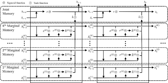
Figure 1: Illustration of mGRN.

As implied by traditional statistical time series models, the multivariate time series’s internal structure can be split to self-dependent components of each variable group, and the interactive component among variables. However, in a vanilla LSTM or GRU, it relies on the neural network to figure out the internal structure. In mGRN, we set up marginal-memory components to extract the group-specific information and a joint-memory component for the joint information, respectively. By explicitly setting up the components, the task of neural networks is simplified.

The mGRN architecture is as follows. An illustration is given in Figure 1.

The marginal-memory component. Suppose the multivariate time series $X_{t}$ is divided into $K$ groups, i.e. $X_{t}=[X^{(1)}_{t},\dots,X^{(K)}_{t}]$, where each $X^{(k)}_{t}$ consists of $m_{k}$ variables with $\sum_{k=1}^{K}m_{k}=M$. Marginal-memory components are formulated in the form of GRU. Given the component dimension $N_{k}$, the $k$-th marginal component contains the candidate memory $\tilde{h}^{(k)}\in\mathbb{R}^{N_{k}\times 1}$ and the final memory $h^{(k)}\in\mathbb{R}^{N_{k}\times 1}$, which are controlled by their own reset gate $r^{(k)}\in\mathbb{R}^{N_{k}\times 1}$ and update gate $z^{(k)}\in\mathbb{R}^{N_{k}\times 1}$.

$$r^{(k)}_{t}=\sigma\left(W^{(k)}_{r}X^{(k)}_{t}+U^{(k)}_{r}h^{(k)}_{t-1}+b^{(k)}_{r}\right),$$

$$z^{(k)}_{t}=\sigma\left(W^{(k)}_{z}X^{(k)}_{t}+U^{(k)}_{z}h^{(k)}_{t-1}+b^{(k)}_{z}\right),$$

$$\tilde{h}^{(k)}_{t}=\tanh\left(W^{(k)}_{h}X^{(k)}_{t}+r^{(k)}_{h}\odot\left(U^{(k)}_{h}h^{(k)}_{t-1}\right)+b^{(k)}_{h}\right),$$

$$h^{(k)}_{t}=\left(1-z^{(k)}_{t}\right)\odot h^{(k)}_{t-1}+z^{(k)}_{t}\odot\tilde{h}^{(k)}_{t}.$$

The trainable parameters are $W^{(k)}_{r}$, $W^{(k)}_{z}$, $W^{(k)}_{h}\in\mathbb{R}^{N_{k}\times M_{k}}$, $U^{(k)}_{r}$, $U^{(k)}_{z}$, $U^{(k)}_{h}\in\mathbb{R}^{N_{k}\times N_{k}}$, and $b^{(k)}_{r}$, $b^{(k)}_{z}$, $b^{(k)}_{h}\in\mathbb{R}^{N_{k}\times 1}$.

The joint-memory component. The joint-memory component is constructed as follows. Given the component dimension $N$, we combine the marginal candidate memories $\{\tilde{h}^{(k)}\}_{k=1}^{K}$ to form the joint candidate memory $\tilde{h}\in\mathbb{R}^{N\times 1}$ as

$$\tilde{h}_{t}=\tanh\left(\sum_{k=1}^{K}U^{(k)}_{c}\tilde{h}^{(k)}_{t}+b_{c}\right).$$

We then add a joint update gate $z\in\mathbb{R}^{N\times 1}$ to regulate the final full output memory $h$ as

$$z_{t}=\sigma(W_{z}X_{t}+U_{z}h_{t-1}+b_{z}),$$

$$h_{t}=(1-z_{t})\odot h_{t-1}+z_{t}\odot\tilde{h}_{t},$$

In this component, the trainable parameters are $W_{z}\in\mathbb{R}^{N\times M}$, $U^{(k)}_{c}\in\mathbb{R}^{N_{k}\times N}$, $U_{z}\in\mathbb{R}^{N\times N}$ and $b_{c}$, $b_{z}\in\mathbb{R}^{N\times 1}$.

There are a few remarks regrading the mGRN architecture.

1. The marginal-memory components only involve group-specific inputs and memories. The network does not need to pick up input-memory correspondence from the mixed data as in vanilla LSTM or GRU.

2. We expose the candidate marginal memories $\{\tilde{h}^{(k)}\}_{k=1}^{K}$, instead of the final marginal memories $\{h^{(k)}\}_{k=1}^{K}$, to the joint component. Our intuition is to give the joint component only the new information. The joint component has its own memory and updates gate to determine which part of the new information is useful.

3. Compared with vanilla GRU and LSTM, separately handling marginal and joint memories will inevitably lead to more intermediate gates. To avoid unnecessarily large models, we take a conservative approach in the design of mGRN. Instead of LSTM, we choose GRU as the building block since GRU achieves comparable performance (Chung et al. 2014) with fewer gates. Instead of using a GRU layer as the joint component, we pick up gates that are crucial to the performance through preliminary experiments. As a result, given the same number of trainable parameters, gates in mGRN have greater sizes comparing with channel-wise LSTM. It is interesting to note that the simplified gates improve model performance not only in the case that the total number of trainable parameters is controlled (see Section 4), but also in the case that all hyperparameters are free to tune.

4. Channel-wise LSTM artificially doubles the features by reversing the input time series. We purposely exclude the step in mGRN to avoid the confusion that the improvements of mGRN may come from reversing the inputs. The technique can be applied to augment any algorithms. In fact, mGRN outperforms channel-wise LSTM even without the extra step; see Section 4 and 5.1.

5. In the traditional time series models such as ARMA, self-dependence is usually limited to a single variable. In mGRN, we extend the scope of self-dependence to a variable group. The internal structures of data sets suggest the extension. For example, in the MIMIC-III data sets in Section 5.1, each variable is coupled with a binary variable to indicate whether it is observed at the step or not. It is intuitive to include the primary variable and the indicative variable in the same group. In the case that the domain knowledge is inadequate to determine variable grouping, we recommend starting from a total split of all variables, which usually gives a satisfactory performance in our experiments. In practice, variable grouping can be regarded as a step of hyperparameter tuning.

6. Following the settings of channel-wise LSTM, in all experiments, the dimensions of marginal components are chosen to be the same, i.e. we choose $\tilde{N}$ such that $N_{k}=\tilde{N}$ for all $k$. Moreover, the joint memory dimension is chosen relative to $\tilde{N}$. We tune a variable $\lambda$ with $N=\lambda\tilde{N}$. In most experiment cases, mGRN performs the best with $\lambda=2$ or $\lambda=4$, i.e. the joint component should be much greater than marginal components.

7. In this paper, we purposely keep the architecture simple to emphasize on the impressive improvements brought by learning marginal and joint memories separately. The architecture can be readily augmented with other components such as CNN and the attention mechanism. To explore the combinations so that the model performance can be maximized will be our future research.

4 Simulation Experiments

In this section, we present a prediction task based on simulated time series. The task is specially designed such that a good prediction requires learning of both marginal and joint serial dependence. Despite both channel-wise LSTM and mGRN are designed for this task, mGRN demonstrates consistent improvements.

4.1 Data Generation Process

The data generation process is taken from Yan, Wu, and Zhang (2019), but with modifications to allow both idiosyncratic and joint serial dependence. To be specific, we generate two correlated series given by

$$y_{i}(t)= \alpha_{i}(t)+\beta_{i}(t)g(\omega_{M}(t);u_{M,i}(t),v_{M,i}(t))$$ (1)

$$+\gamma_{i}(t)g(\omega_{i}(t);u_{i}(t),v_{i}(t)),\quad\text{for}\quad i=1,2,$$

where $g(\omega;u,v):=\omega(u^{\omega}/A+v^{-\omega}/A+1)$ with $A=4$ and $u\geq 0$, $v\geq 0$. $\omega_{M}(t)$ and $\omega_{i}(t)$ are independent with common distribution $\mathcal{N}(0,1)$.

The parameters have serial-dependent dynamics given by the following AR(5) process

$$p(t)= \mu_{p}+0.9p(t-1)-0.8p(t-2)+0.7p(t-3)-$$ (2)

$$0.6p(t-4)+0.5p(t-5)+\epsilon_{p}(t)$$

$$\text{for }p= \alpha_{i},\log{\beta_{i}},\log{u_{M,i}},\log{v_{M,i}},\log{\gamma_{i}},\log{u_{i}},\log{v_{i}},$$

$$i= 1,2,$$

where the random noises $\epsilon_{p}(t)$ are independent with common distribution $\mathcal{N}(0,0.01)$. Note that we take the logarithm of parameters other than $\alpha$ to ensure positivity.

The coefficients of the AR processes (2) are arbitrarily fixed except for the constant terms, which are chosen to generate realistic time series. Table 2 of Yan, Wu, and Zhang (2019) reports the parameters of a few stocks. $y_{1}$ and $y_{2}$ are matched with a pair of stocks in the table. $\mu_{\alpha_{i}}$ is selected so that $E[\alpha_{i}(t)]$ matches with the corresponding parameter. For $p=\log{\beta_{i}}$ and $\log{\gamma_{i}}$, $\mu_{p}$ is chosen such that $\exp{E[p(t)]}$ matches with one tenth of the corresponding parameter. For $p=\log{u_{M,i}},\log{v_{M,i}},\log{u_{i}}$ and $\log{v_{i}}$, $\mu_{p}$ is chosen such that $\exp{E[p(t)]}$ matches with the corresponding parameter. To guarantee the robustness of the results, we repeat experiments with 10 pairs of randomly selected stocks.

The simulation process (1) is proposed initially to capture the extremal dependence among financial assets. We adopt this model in the simulation study for a few reasons. Firstly, it explicitly sets up an idiosyncratic component and a correlated component, which match with the structures of mGRN. Moreover, it provides the simulated data with adequate complexity, such as randomness, heavy-tailless and time-varying distributions, all of which are commonly observed in real-world data sets.

4.2 Analysis of the Prediction Task

The task is to jointly predict $100\times y_{1}(t)\times y_{2}(t)$ given observations up to step $t-1$. We choose the loss function to be mean squared error (MSE), so that there is a theoretical best predictor $E[100y_{1}(t)y_{2}(t)|\mathcal{F}_{t-1}]$ (Shumway and Stoffer 2017). Thanks to the Gaussian conditional distributions of AR processes (2), the best predictor can be explicitly evaluated.

We postpone the tedious evaluation of the best predictor $E[100y_{1}(t)y_{2}(t)|\mathcal{F}_{t-1}]$ to Appendices, and focus on the implications. First, the best predictor enjoys a closed-form minimum MSE. It provides valuable information about how much the prediction results can be improved. In particular, due to the existence of randomness, the minimum MSE is much greater than $0$.

Second, the best predictor is indeed a complicated function of $E[\alpha_{i}(t)|\mathcal{F}_{t-1}]$, $E[\beta_{i}(t)|\mathcal{F}_{t-1}]$, $E[u_{M,i}(t)|\mathcal{F}_{t-1}]$, $E[v_{M,i}(t)|\mathcal{F}_{t-1}]$, $E[\gamma_{i}(t)|\mathcal{F}_{t-1}]$, $E[u_{i}(t)|\mathcal{F}_{t-1}]$ and $E[v_{i}(t)|\mathcal{F}_{t-1}]$ for $i=1,2$. Note that, under the AR processes (2),

$$E[p(t)|\mathcal{F}_{t-1}]= \mu_{p}+0.9p(t-1)-0.8p(t-2)+$$ (3)

$$0.7p(t-3)-0.6p(t-4)+0.5p(t-5).$$

As a result, a good prediction requires the neural network to pick up the past dependence in the individual series, as well as the function to combine the marginal information.

4.3 Experiment Settings and Results

To make predictions, we include observations of the past 5 steps in neural networks. Apart from $y_{i}$, parameter series ($\alpha_{i},\beta_{i}$ and so on) are also fed into neural networks, leading the total input dimension $M$ to be 16.

We test two intuitive ways to group the variables. The first way is to split the variables to two groups, each of which contains $y_{i}$ together with its parameters, i.e. $m_{1}=m_{2}=8$. Since each $y_{i}$ is jointly determined by its parameters, it may not be wise to break the connections. The second grouping is suggested by the best predictor. The variables are totally split into 16 groups so that there is a marginal component to learn each marginal conditional expectation (3).

Model	MSE	Relative difference
		with
		theoretical minimum
LSTM	22.26	2.87%
GRU	22.20	2.59%
Channel-wise LSTM	22.06	1.94%
(two groups)
Channel-wise LSTM	21.93	1.34%
(total split)
mGRN (two groups)	21.91	1.25%
mGRN (total split)	21.88	1.11%
Theoretical minimum	21.64	-

Table 1: The average mean squared error (MSE) in the base case of the simulation experiment. The average is taken across the simulation paths generated from 10 pairs of parameters reported in Yan, Wu, and Zhang (2019). The theoretical minimum MSE is calculated with the best predictor $E[100y_{1}(t)y_{2}(t)|\mathcal{F}_{t-1}]$. Smaller MSEs indicate better predictions. A relative difference is calculated as (model MSE - theoretical minimum)/theoretical minimum. The bold numbers are the best results.

A total number of $100,000$ observations are generated for each simulation path. The first $70,000$ observations are used to train models. The next $15,000$ observations are used for validation. The final performance is evaluated in the last $15,000$ observations. As mentioned earlier, all experiments are repeated with 10 pairs of randomly selected stocks reported in Yan, Wu, and Zhang (2019).

In this simulation experiment, we compare the proposed model with a few recurrent neural networks, namely, LSTM, GRU, and channel-wise LSTM. An advantage of mGRN relative to channel-wise LSTM is that it uses variables efficiently by setting up fewer gates. To demonstrate the advantage, we limit the total number of trainable parameters to be around 1.8 thousand for all models. The number is chosen such that further increases of the model sizes do not improve validation results for LSTM or GRU. For both channel-wise LSTM and mGRN, we tune $\lambda$ (as mentioned earlier, we set $N=\lambda\tilde{N}$) via grid searches within $\{1,2,4,8\}$. The marginal and joint dimensions ($\tilde{N}$ and $N$) are adjusted accordingly. Note that it is impossible to set the numbers of trainable parameters to be exactly the same for all models. In general, we choose the number of parameters of mGRN to be smaller than those of alternative models. We also tune the learning rates via grid searches within $\{10^{-4},5\times 10^{-4},10^{-3}\}$.

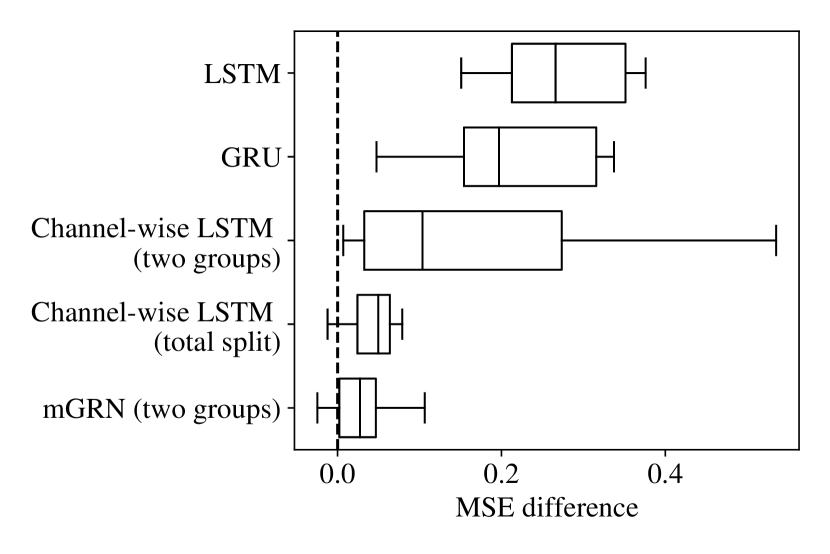
Figure 2: Improvements of mGRN (total split) in MSE comparing to alternative architectures in the simulation experiment. The boxplots are plotted with data simulated from 10 pairs of stock parameters reported in Yan, Wu, and Zhang (2019). The vertical dotted line indicates 0. A positive difference suggests that mGRN (total split) performs better than the corresponding model.

	AUC-ROC	AUC-PR
Logistic regression	0.848	0.474
LSTM	0.855	0.485
Channel-wise LSTM	0.862	0.515
mGRN	0.862	0.523

(a) In-hospital mortality

	AUC-ROC	AUC-PR
Logistic regression	0.870	0.214
LSTM	0.892	0.324
Channel-wise LSTM	0.906	0.333
mGRN	0.911	0.347

(b) Decompensation

	Kappa	MAD
Logistic regression	0.402	162.3
LSTM	0.438	123.1
Channel-wise LSTM	0.442	136.6
mGRN	0.447	124.6

(c) Length of stay

	Macro	Micro
	AUC-ROC	AUC-ROC
Logistic regression	0.739	0.799
LSTM	0.770	0.821
Channel-wise LSTM	0.776	0.825
mGRN	0.779	0.826

(d) Phenotyping

Table 2: Model performance on the MIMIC-III data set (Johnson et al. 2016). Except for those of mGRN, all results are taken from Harutyunyan et al. (2019). Greater values are better for all metrics except mean absolute difference (MAD). The bold numbers are the best results. Following Harutyunyan et al. (2019), the reported results are the mean values calculated by resampling the test sets $Q$ times with replacement ($Q=10000$ for in-hospital mortality prediction and phenotype classification, and $Q=1000$ for decompensation and length-of-stay prediction tasks). $95\%$ confidence intervals are provided in Appendices.

Table 1 gives the average MSE of each model across the 10 simulation paths. We want to emphasize that the improvements of mGRN are not only in the average sense; it outperforms alternative models in almost all simulation cases, as shown in figure 2, which gives the MSE improvements of mGRN (total split).

There are a few observations. First, both mGRN and channel-wise LSTM perform significantly better than vanilla LSTM and GRU. This is not surprising, as mGRN and channel-wise LSTM are designed for the task. It is more interesting to notice that mGRN performs consistently better than channel-wise LSTM. This suggests that mGRN performs better at picking up the marginal and joint serial dependence.

A second observation is that predictions are better when variables are totally split. This is consistent with the structure of the best predictor. However, without the best predictor, the result may not be intuitive, as it seems to be unwise to break the tight connections between $y_{i}$ and its parameters. Of course, there will not be a best predictor to suggest variable grouping. Once again, this may be regarded as a step of hyperparameter tuning, and to totally split the variables may be a good first attempt.

5 Real-world Applications

In this section, we evaluate the performance of mGRN on real-world data sets. The data sets, together with the results of the state-of-the-art models’, are borrowed from Harutyunyan et al. (2019) and Zhang et al. (2020). All data sets are publicly available. All results, except for those of mGRN, are taken from the two papers. To obtain the results of mGRN, we strictly follow the original experiment settings and perform grid searches on hyperparameters such as variable grouping, dimensions of the marginal and joint components ($\tilde{N}$ and $N$), learning rates, and dropouts. Experiments are coded with Pytorch (Paszke et al. 2019) and performed on NVIDIA TITAN Xp GPUs with 12 GB memory. Please refer to Appendices for the codes and pre-trained models to reproduce the results.

5.1 MIMIC-III Data Set

Harutyunyan et al. (2019) reports the performance of logistic regression, LSTM, and channel-wise LSTM on the Medical Information Mart for Intensive Care (MIMIC-III) data set (Johnson et al. 2016), which consists of multivariate time series of intensive care unit (ICU) records. Raised from real-world applications, the data set contains common difficulties such as missing values and highly skewed responses.

In their experiments, Harutyunyan et al. (2019) uses 17 clinical variables, including both continuous and categorical types. Categorical variables are encoded in one-hot format. Moreover, each variable is coupled with a binary variable to indicate whether the corresponding variable is observed or not. In total, the input dimension $M$ is 76. Following the variable grouping of channel-wise LSTM, we group each clinical variable with the corresponding indicative binary variable, leading to 17 variable groups.

	mGRN	TapNet	MLSTM	WEASEL	ED	DTW	DTW	ED-1NN	DTW-1NN	DTW-1NN
			-FCN	+MUSE	-1NN	-1NN-I	-1NN-D	(norm)	-I (norm)	-D (norm)
CT	0.995*	0.997	0.985	0.990	0.964	0.969	0.990	0.964	0.969	0.989
FD	0.596	0.556*	0.545	0.545	0.519	0.513	0.529	0.519	0.500	0.529
LSST	0.614	0.568	0.373	0.590*	0.456	0.575	0.551	0.456	0.575	0.551
PD	0.989	0.980*	0.978	0.948	0.973	0.939	0.977	0.973	0.939	0.977
PS	0.227	0.175	0.110	0.190*	0.104	0.151	0.151	0.104	0.151	0.151
SAD	0.997	0.983	0.990*	0.982	0.967	0.960	0.963	0.967	0.959	0.963

Table 3: Classification accuracy on UEA data sets (Bagnall et al. 2018). We focus on the data sets whose training samples are greater than $1000$. They are character trajectories (CT), face detection (FD), LSST, pen digits (PD), phoneme spectra (PS), and spoken Arabic digits (SAD). Except for those of mGRN, all results are taken from Zhang et al. (2020). Greater values indicate better classification. The bold numbers are the best results. The second best results are labeled by asterisks.

Harutyunyan et al. (2019) proposes the following four benchmark health care problems:

1. In-hospital-mortality prediction. To predict in-hospital mortality marking use of ICU records in the first 48 hours. This is a binary classification task.

2. Decompensation prediction. To predict the mortality of a patient in the next 24 hours making use of all the available ICU records. This is a binary classification task.

3. Length-of-stay prediction. To predict the remaining number of days of a patient in the ICU making use of all the available ICU records. The task is a multi-category classification task.

4. Phenotype classification. To classify which of 25 acute care conditions are present given the full ICU records. This task is a combination of 25 binary classification tasks.

As given in table 2, classification results are evaluated with multiple metrics, such as the area under the receiver operator characteristic curve (AUC-ROC) and area under the precision-recall curve (AUC-PR), since the labels are highly skewed (Davis and Goadrich 2006). The total number of samples greatly varies among tasks, ranging from 18 thousand to 3 million. We follow the default training-validation-test split. For more details about the data set and experiment setup, please refer to Harutyunyan et al. (2019).

Experiment results are reported in table 2. Except for those of mGRN, all results are taken from Harutyunyan et al. (2019). mGRN demonstrates consistent improvements compared with the strong baselines. In particular, benefiting from the deliberately designed gates and information flows, mGRN outperforms channel-wise LSTM even though the two models share a similar intuition. The improvements are the most significant in decompensation prediction and length-of-stay prediction. These two tasks have much greater training samples (around 2 million samples) than the other two tasks (less than 25 thousand samples). Note that, as mentioned earlier, channel-wise LSTM may have gained from doubling the inputs by reversing them, which we purposely exclude from mGRN to avoid confusion.

5.2 UEA Data Sets

Zhang et al. (2020) conducts experiments on UEA multivariate time series data sets (Bagnall et al. 2018). We omit the data sets whose training samples are small and focus on those whose training samples are greater than $1000$. They are character trajectories (CT), face detection (FD), LSST, pen digits (PD), phoneme spectra (PS), and spoken Arabic digits (SAD). In these data sets, the number of variables ranges from 2 to 144, and the time series length ranges from 8 to 217. All tasks are multivariate classification evaluated with classification accuracy. Following Zhang et al. (2020), the data sets are only split to training sets and test sets.

The results reported in Zhang et al. (2020) comprise a few state-of-the-art algorithms targeting multivariate time series. The algorithms are either extensions of traditional machine learning techniques (ED-I, DTW-I, DTW-D, and WEASEL+MUSE) or novel neural networks (MLSTM-FCN and TapNet). In particular, ED-I, DTW-I, and DTW-D are applied to the data sets with (as labeled by ”norm”) or without normalization. Please refer to Zhang et al. (2020) for more information about the data sets and experiment setup.

Experiment results are reported in table 3. Except for those of mGRN, all results are taken from Zhang et al. (2020). mGRN dramatically improves classification accuracy on almost all data sets. The greatest improvement is found on the face detection data set. Compared to the second-best result (TapNet), mGRN increases the classification accuracy by $4\%$. The only exception is the character trajectories data set, in which the room to improve is tiny.

6 Conclusion

This paper presents an RNN architecture called Memory-Gated Recurrent Network (mGRN) for the multivariate time series analysis. Motivated by traditional time series models, we introduce separate gates to regulate marginal and joint memories of variables. To be specific, for each variable group, we set up a marginal-memory component in the form of GRU to extract group-specific dependence. Each group’s candidate memory is then combined in the joint-memory component to capture interactions among variable groups. Through a combination of comprehensive simulation studies and empirical experiments on a range of public datasets, we show that our proposed mGRN architecture consistently outperforms state-of-the-art architectures targeting multivariate time series. To further improve the architecture performance by combining with other techniques such as CNN and the attention mechanism will be our future research.

References

- Bagnall et al. (2018) Bagnall, A.; Dau, H. A.; Lines, J.; Flynn, M.; Large, J.; Bostrom, A.; Southam, P.; and Keogh, E. 2018. The UEA multivariate time series classification archive, 2018. arXiv preprint arXiv:1811.00075 .
- Baydogan and Runger (2015) Baydogan, M. G.; and Runger, G. 2015. Learning a symbolic representation for multivariate time series classification. Data Mining and Knowledge Discovery 29(2): 400–422.
- Baydogan and Runger (2016) Baydogan, M. G.; and Runger, G. 2016. Time series representation and similarity based on local autopatterns. Data Mining and Knowledge Discovery 30(2): 476–509.
- Belletti et al. (2018) Belletti, F.; Beutel, A.; Jain, S.; and Chi, E. 2018. Factorized recurrent neural architectures for longer range dependence. In International Conference on Artificial Intelligence and Statistics, 1522–1530.
- Chakraborty et al. (1992) Chakraborty, K.; Mehrotra, K.; Mohan, C. K.; and Ranka, S. 1992. Forecasting the behavior of multivariate time series using neural networks. Neural networks 5(6): 961–970.
- Cho et al. (2014) Cho, K.; Van Merriënboer, B.; Bahdanau, D.; and Bengio, Y. 2014. On the properties of neural machine translation: Encoder-decoder approaches. arXiv preprint arXiv:1409.1259 .
- Chung et al. (2014) Chung, J.; Gulcehre, C.; Cho, K.; and Bengio, Y. 2014. Empirical evaluation of gated recurrent neural networks on sequence modeling. arXiv preprint arXiv:1412.3555 .
- Davis and Goadrich (2006) Davis, J.; and Goadrich, M. 2006. The relationship between Precision-Recall and ROC curves. In Proceedings of the 23rd international conference on Machine learning, 233–240.
- Harutyunyan et al. (2019) Harutyunyan, H.; Khachatrian, H.; Kale, D. C.; Ver Steeg, G.; and Galstyan, A. 2019. Multitask learning and benchmarking with clinical time series data. Scientific data 6(1): 1–18.
- Hochreiter and Schmidhuber (1997) Hochreiter, S.; and Schmidhuber, J. 1997. Long short-term memory. Neural computation 9(8): 1735–1780.
- Johnson et al. (2016) Johnson, A. E.; Pollard, T. J.; Shen, L.; Li-Wei, H. L.; Feng, M.; Ghassemi, M.; Moody, B.; Szolovits, P.; Celi, L. A.; and Mark, R. G. 2016. MIMIC-III, a freely accessible critical care database. Scientific data 3(1): 1–9.
- Karim et al. (2017) Karim, F.; Majumdar, S.; Darabi, H.; and Chen, S. 2017. LSTM fully convolutional networks for time series classification. IEEE access 6: 1662–1669.
- Karim et al. (2019) Karim, F.; Majumdar, S.; Darabi, H.; and Harford, S. 2019. Multivariate LSTM-FCNs for time series classification. Neural Networks 116: 237–245.
- Karlsson, Papapetrou, and Boström (2016) Karlsson, I.; Papapetrou, P.; and Boström, H. 2016. Generalized random shapelet forests. Data mining and knowledge discovery 30(5): 1053–1085.
- Ling and McAleer (2003) Ling, S.; and McAleer, M. 2003. Asymptotic theory for a vector ARMA-GARCH model. Econometric theory 280–310.
- Lipton, Berkowitz, and Elkan (2015) Lipton, Z. C.; Berkowitz, J.; and Elkan, C. 2015. A critical review of recurrent neural networks for sequence learning. arXiv preprint arXiv:1506.00019 .
- Ma et al. (2017) Ma, F.; Chitta, R.; Zhou, J.; You, Q.; Sun, T.; and Gao, J. 2017. Dipole: Diagnosis prediction in healthcare via attention-based bidirectional recurrent neural networks. In Proceedings of the 23rd ACM SIGKDD international conference on knowledge discovery and data mining, 1903–1911.
- Paszke et al. (2019) Paszke, A.; Gross, S.; Massa, F.; Lerer, A.; Bradbury, J.; Chanan, G.; Killeen, T.; Lin, Z.; Gimelshein, N.; and Antiga, L. 2019. Pytorch: An imperative style, high-performance deep learning library. In Advances in neural information processing systems, 8026–8037.
- Quenouille (1957) Quenouille, M. H. 1957. The analysis of multiple time-series. Technical report, Griffin London.
- Schäfer and Leser (2017) Schäfer, P.; and Leser, U. 2017. Multivariate time series classification with WEASEL+ MUSE. arXiv preprint arXiv:1711.11343 .
- Shokoohi-Yekta, Wang, and Keogh (2015) Shokoohi-Yekta, M.; Wang, J.; and Keogh, E. 2015. On the non-trivial generalization of dynamic time warping to the multi-dimensional case. In Proceedings of the 2015 SIAM international conference on data mining, 289–297. SIAM.
- Shumway and Stoffer (2017) Shumway, R. H.; and Stoffer, D. S. 2017. Time series analysis and its applications: with R examples. Springer.
- Tai, Socher, and Manning (2015) Tai, K. S.; Socher, R.; and Manning, C. D. 2015. Improved semantic representations from tree-structured long short-term memory networks. arXiv preprint arXiv:1503.00075 .
- Tsay (2005) Tsay, R. S. 2005. Analysis of financial time series, volume 543. John wiley & sons.
- Tuncel and Baydogan (2018) Tuncel, K. S.; and Baydogan, M. G. 2018. Autoregressive forests for multivariate time series modeling. Pattern recognition 73: 202–215.
- Yan, Wu, and Zhang (2019) Yan, X.; Wu, Q.; and Zhang, W. 2019. Cross-sectional Learning of Extremal Dependence among Financial Assets. In Advances in Neural Information Processing Systems, 3852–3862.
- Zhang et al. (2020) Zhang, X.; Gao, Y.; Lin, J.; and Lu, C.-T. 2020. TapNet: Multivariate Time Series Classification with Attentional Prototypical Network. In AAAI, 6845–6852.