Dependence of variance on covariate design in nonparametric link regression

Abstract

This paper discusses a design-dependent nature of variance in nonparametric link regression aiming at predicting a mean outcome at a link, i.e., a pair of nodes, based on currently observed data comprising covariates at nodes and outcomes at links.

1 Introduction

Binary link prediction in node-attributed graphs (Taskar et al.,, 2003; Menon and Elkan,, 2011) is the task of predicting the link existence from the corresponding node covariates. It has attracted widespread and long-standing interest in a wide range of applied areas such as social science studies (Gong et al.,, 2014). The binary link prediction is generalized to similarity learning (Liu et al.,, 2015; Kulis,, 2012; Pinheiro,, 2018), which aims at predicting possibly non-binary outcomes (representing similarity) defined between two node covariates. Similarity learning is classified into two types depending on whether node covariates come from a single domain (Liu et al.,, 2015) or two different domains (Pinheiro,, 2018). The former setting is theoretically interesting as it assumes symmetry of similarity. In the single-domain setting, Okuno and Shimodaira, (2020) and Graham, (2020) consider parametric regression for predicting real-valued outcomes from covariates. Regression for learning similarity in the single-domain setting is called link regression.

This paper focuses on a nonparametric approach to link regression that predicts mean outcomes at links of size $n(n-1)/2$ based on node covariates of size $n$. We show that the decay rate of the deterministic bias with respect to a bandwidth parameter and the sample size remains the same regardless of whether the designs of node covariates are fixed (i.e., fixed design) or randomly obtained (i.e., random design), whereas that of the stochastic variance drastically differs depending on covariates’ designs. This dependence comes from the conditional bias due to the randomness of covariates in random design cases. The conditional bias behaves like the non-degenerate $U$-statistics (Lee,, 1990) and is controlled by the sample size of independent node covariates. Figure 1(1) showcases a numerical result demonstrating this theoretical finding in comparison to conventional nonparametric regression. At the same time, this study demonstrates that there exists a threshold value, below which the difference between two designs disappears. In particular, the variance decay rates in both designs match for the bandwidth alleviating the bias-variance trade-off.

The distinction between the fixed and random designs in regression has been addressed in the literature on statistics and machine learning. Fixed design analysis is common when covariates are physically controlled, while random design analysis is conducted when the values of covariates are unpredictable. These designs are fundamentally different as discussed in Györfi et al., (2002). Brown, (1990) has displayed the design-dependent nature of the statistical decision theory in parametric regression models. Buja et al., (2019) has demonstrated that the randomness of covariates produces additional variance of parametric regression estimates. However, in nonparametric regression, the difference in the decay rates of bias and variance between fixed and random designs is known to appear only in a multiplicative constant (e.g., Hardle,, 1990; Fan,, 1992; Györfi et al.,, 2002), implying the negligibility of the difference in a usual asymptotic framework (Figure 1(1)). The situation drastically changes in nonparametric link regression as pairs of node covariates are dependent (despite outcomes at links being independent), and the difference cannot be ignored.

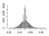
A

Nonparametric link regression estimate

$\widehat{f}_{n,h}(x,x^{\prime})$ at a query $(x,x^{\prime})=(0.5,0.5)$.

B

Nonparametric regression estimate

$\widehat{f}_{n,h}(x)$ at a query $x=0.5$.

Figure 1: Histograms of the values of estimates under univariate random and fixed designs: (1) a kernel smoother for $f(x,x^{\prime})=\mathbb{E}(Y\mid X=x,X^{\prime}=x^{\prime})=xx^{\prime}$ defined in (1). (1) a kernel smoother for $f(x)=\mathbb{E}(Y\mid X=x)=x$. For both experiments, 500 covariates were employed and the bandwidth was set to $h=h_{n}:=n^{-1/(d+3)}$ as the Hölder smoothness of $f$ is $\beta=1$.

1.1 Notations

The following notation is adopted throughout this paper. Let $\mathcal{X}$ be a compact subset of $\mathbb{R}^{d}$ and $\mathcal{Y}$ be a subset of $\mathbb{R}$. Let $\|\cdot\|$ denote the Euclidean norm of $\mathbb{R}^{d}$. For two sequences $\{a_{n,h}\}_{n\in\mathbb{N},h>0}$ and $\{b_{n,h}\}_{n\in\mathbb{N},h>0}$ the notation $a_{n,h}=O(b_{n,h})$ indicates that there exists an absolute constant $c>0$ for which $a_{n,h}\leq c\cdot b_{n,h}$. Operations $\mathbb{E}[\cdot]$ and $\operatorname{Var}[\cdot]$ denote taking expectation and variance, respectively. For a conditional expression $\mathcal{S}$, $\mathbbm{1}_{\mathcal{S}}$ denotes an indicator function taking the value of 1 if and only if $\mathcal{S}$ is satisfied and 0 otherwise. For a set $A$, $|A|$ denotes the number of elements in the set.

2 Nonparametric link regression

Suppose that given node covariates $\{X_{i}\in\mathcal{X}:i=1,\ldots,n\}$, symmetric outcomes $Y_{i_{1},i_{2}}=Y_{i_{2},i_{1}}\in\mathcal{Y}$ independently follow a conditional distribution $Q(Y_{i_{1},i_{2}}\mid X_{i_{1}},X_{i_{2}})$ for $1\leq i_{1}<i_{2}\leq n$. Our aim is to estimate the symmetric conditional mean of $Y\mid X,X^{\prime}\sim Q$ at a query $(x,x^{\prime})$

$$f(x,x^{\prime}):=\mathbb{E}[Y\mid X=x\,,\,X^{\prime}=x^{\prime}]$$

on the bases of the observations $\{(Y_{i_{1},i_{2}},X_{i_{1}},X_{i_{2}})\in\mathcal{Y}\times\mathcal{X}^{2}:(i_{1},i_{2})\in I_{n}\}$ with an index set $I_{n}:=\{(i_{1},i_{2}):1\leq i_{1}\neq i_{2}\leq n\}$. In this study, the symmetric conditional mean is called a link regression function. Consider nonparametric estimation over the link regression function. In this study, the following kernel smoother is used for the link regression function $f$:

$$\widehat{f}_{n,h}(x,x^{\prime}) :=\frac{|I_{n}|^{-1}\sum_{(i_{1},i_{2})\in I_{n}}Y_{i_{1}i_{2}}\{K_{h}(x-X_{i_{1}})K_{h}(x^{\prime}-X_{i_{2}})+\lambda_{n}\}}{|I_{n}|^{-1}\sum_{(i_{1},i_{2})\in I_{n}}\{K_{h}(x-X_{i_{1}})K_{h}(x^{\prime}-X_{i_{2}})+\lambda_{n}\}},$$ (1)

where $K_{h}(\cdot):=h^{-d}K(\cdot/h)$ with a bandwidth $h>0$ and a $d$-variate kernel $K$, and $\lambda_{n}$ is a regularization parameter. Regularization is applied to the denominator as suggested by Fan, (1993) to prevent it from becoming zero. Furthermore, the term $\lambda_{n}$ is added to the nominator for the kernel smoother to keep the form of the weighted average of outcomes.

In our theory, the bandwidth $h=h_{n}$ and the regularization parameter $\lambda_{n}$ are assumed to satisfy

$$n^{-1/d}\leq h\leq 1,\qquad\frac{1}{(nh^{d})^{\nu}}\leq\lambda_{n}\leq h^{d}$$ (2)

for some $\nu>0$; this condition yield inequalities $1\leq nh^{d}$ and $1/\{\lambda_{n}(nh^{d})^{\nu}\}\leq 1$, and the condition is satisfied by $\lambda_{n}=n^{-1}$ with the optimal bandwidth $h=n^{-1/(\beta+d)}$ obtained in Theorem 2.3.

It is well-known that the kernel smoother has a limitation to attaining the optimal rate of convergence for function classes with higher order smoothness (Ruppert and Wand, (1994)); this limitation is alleviated by local polynomial regression. As the extension to local polynomial regression is straightforward in nonparametric link regression, it is not considered in this paper for the ease of notation.

2.1 Theoretical result

Properties of the kernel smoother $\widehat{f}_{n,h}$ are derived, with the following conditions imposed on the true link regression function $f$, conditional variance $\sigma$, kernel $K$ and the covariate $X$.

Condition 2.1.

The following hold:

1. The link regression function $f(x,x^{\prime})$ is contained in $\mathcal{F}(\beta,L)$ with $0<\beta\leq 1$ and $L>0$ defined as $\mathcal{F}(\beta,L):=\left\{f:|f(x,x^{\prime})-f(\widetilde{x},x^{\prime})|\leq L\|x-\widetilde{x}\|^{\beta},\,|f(x,x^{\prime})|\leq L\,,\,x,\widetilde{x},x^{\prime}\in\mathcal{X}\right\}$;

2. There exists $\tau>0$ for which $\sigma^{2}(x,x^{\prime}):=\operatorname{Var}[Y\mid X=x,\,X^{\prime}=x^{\prime}]<\tau$ for $x,x^{\prime}\in\mathcal{X}$.

Condition 2.2.

The following hold:

1. The $d$-variate kernel $K(z)$ is a compactly supported, symmetric, bounded density function with a mean of zero and $K_{\mathrm{max}}:=\sup_{z}K(z)$, and has the finite second moment;

2. There exist $\underline{k}>0$ and $r>0$ for which $\underline{k}\cdot\sup_{z}K(z)\leq\inf_{z:\|z\|\leq r}K(z)$.

Condition 2.3.

One of the following holds:

1. $\{X_{i}:i=1,2,\ldots,n\}$ is a deterministic triangular array that satisfies $c_{X}/n^{1/d}\leq\min_{i,j}\|X_{i}-X_{j}\|\leq\max_{i}\min_{j}\|X_{i}-X_{j}\|\leq C_{X}/n^{1/d}$ for some $c_{X},C_{X}>0$;

2. $\{X_{i}:i=1,2,\ldots,n\}$ is an array of independent and identically distributed (i.i.d.) random variables from the marginal density $m$, where $m$ is continuous and bounded from both above and below: $0<l\leq m(x)\leq u<\infty$.

Condition 2.1 specifies the smoothness of the link regression function $f$. A larger $\beta$ yields a smoother function $f$, which is easier to estimate. Condition 2.2 is mild and satisfied by a large variety of kernels such as the boxcar and Epanechnikov kernels. Condition 2.3 (a) makes covariates nearly equispaced. Condition 2.3 (b) is a mild condition; for example, the uniform distribution over $\mathcal{X}$ satisfies this condition. Hereafter, we call Conditions 2.3 (a) and 2.3 (b) as the fixed and random designs, respectively. Let

$$\rho_{1}(n,h) :=\sup_{f\in\mathcal{F}(\beta,L)}\left|f(x,x^{\prime})-\mathbb{E}\left[\widehat{f}_{n,h}(x,x^{\prime})\right]\right|^{2},$$

$$\rho_{2}(n,h) :=\sup_{f\in\mathcal{F}(\beta,L)}\mathbb{E}\left[\operatorname{Var}\left[\widehat{f}_{n,h}(x,x^{\prime})\mid X_{1},X_{2},\ldots,X_{n}\right]\right],$$

$$\rho_{3}(n,h) :=\sup_{f\in\mathcal{F}(\beta,L)}\operatorname{Var}\left[f(x,x^{\prime})-\mathbb{E}\left[\widehat{f}_{n,h}(x,x^{\prime})\mid X_{1},X_{2},\ldots,X_{n}\right]\right]$$

where these terms upper-bound the squared bias and the variance of $\widehat{f}_{n,h}(x,x^{\prime})$ by $\rho_{1}$ and $\rho_{2}+\rho_{3}$, respectively, whereby the overall risk $\mathbb{E}|f(x,x^{\prime})-\widehat{f}_{n,h}(x,x^{\prime})|^{2}$ is upper-bounded by $\rho_{1}+\rho_{2}+\rho_{3}$. These terms $\rho_{1},\rho_{2},\rho_{3}$ are evaluated as follows, with the proof provided in Supplement C.2.

Theorem 2.1.

Assume that Conditions 2.1 and 2.2 are satisfied, and $n^{-1/d}\leq h\leq 1$ and $1/(nh^{d})^{\nu}\leq\lambda_{n}\leq h^{d}$ for some $\nu>0$. Then, there exists a positive constant $C$ not depending on $n$ and $h$, for which the following holds:

• In both cases of Condition 2.3, $\rho_{1}(n,h)\leq Ch^{2\beta}$ and $\rho_{2}(n,h)\leq C(nh^{d})^{-2}$;

• Under Condition 2.3 (a), $\rho_{3}(n,h)=0$; under Condition 2.3 (b), $\rho_{3}(n,h)\leq Ch^{2\beta}(nh^{d})^{-1}$.

With the bandwidth $h=n^{-1/(s+d)}$, Theorem 2.1 yields the following variance evaluation:

$$\operatorname{Var}[\widehat{f}_{n,h}(x,x^{\prime})]=\begin{cases}O\left(n^{-\frac{2s}{s+d}}\right)&\text{ under Condition \ref{condition: design} (a), }\\ O\left(n^{-\frac{\min\{2s,2\beta+s\}}{s+d}}\right)&\text{ under Condition \ref{condition: design} (b). }\end{cases}$$

This implies that the stochastic variance in the random design decays slower than that in the fixed design for $s>2\beta$. This also implies that the decay rates of the stochastic variances in both designs match in the other regimes. Hence, the smoothness misspecification produces a difference in variances with respect to the designs. See also Supplement B for numerical experiments demonstrating the dependence of the variance on the covariate design.

Theorem 2.1 also yields the upper-bound of the risk.

Theorem 2.2.

Assume that Conditions 2.1 and 2.2 are satisfied, $n^{-1/d}\leq h\leq 1$ and $1/(nh^{d})^{\nu}\leq\lambda_{n}\leq h^{d}$ for some $\nu>0$. Then, there exists a positive constant $C$ not depending on $n$ and $h$, for which the following holds:

$$\sup_{f\in\mathcal{F}(\beta,L)}\mathbb{E}|f(x,x^{\prime})-\widehat{f}_{n,h}(x,x^{\prime})|^{2}\leq\begin{cases}C\{h^{2\beta}+(nh^{d})^{-2}\}&\text{under Condition \ref{condition: design} (a)},\\ C\{h^{2\beta}+h^{2\beta}(nh^{d})^{-1}+(nh^{d})^{-2}\}&\text{under Condition \ref{condition: design} (b)}.\end{cases}$$

Combined with the lower bound estimate of the risks, the above evaluation also yields the optimal bandwidth. If the bandwidth $h$ is set to $h=n^{-1/(\beta+d)}$ with a true smoothness $\beta$, the optimal rate of convergence is obtained in both designs.

Theorem 2.3.

Assume that the conditional distribution $Q$ is a normal distribution. In either Condition 2.3 (a) or (b), the kernel smoother with the bandwidth $h=n^{-1/(\beta+d)}$ attains asymptotically minimax optimality

$$\limsup_{n\to\infty}\bigg{\{}\sup_{f\in\mathcal{F}(\beta,L)}\mathbb{E}\left[|f(x,x^{\prime})-\widehat{f}_{n,h}(x,x^{\prime})|^{2}\right]\big{/}\inf_{\widehat{f}_{n}}\sup_{f\in\mathcal{F}(\beta,L)}\mathbb{E}\left[|f(x,x^{\prime})-\widehat{f}_{n}(x,x^{\prime})|^{2}\right]\bigg{\}}<\infty,$$

and the asymptotically minimax risk is of order $n^{-2\beta/(\beta+d)}$ with respect to $n$.

The proof is presented in Supplement C.3. The theorem also holds for cases where the conditional distribution satisfies the conditions in Section 2 of Gill and Levit, (1995); for example, the theorem holds for cases where $Q$ is a Bernoulli distribution and $\mathcal{F}(\beta,L)$ is replaced by $\mathcal{F}(\beta,L)\cap\{f:0<l<\inf f(x,x^{\prime})\leq\sup f(x,x^{\prime})<u<1\}$ with $0<l<u<1$.

Note that, a similar but different result on the variance of the link regression under the random design has been reported recently (Graham et al.,, 2021), independently to this work. Graham et al., (2021) employs the probabilistic model $Y_{ij}=f(X_{i},X_{j})+U_{i}+U_{j}+V_{ij}$ with i.i.d. normal random variables $U_{i},V_{ij}\sim N(0,1)$ while our setting corresponds to $Y_{ij}=f(X_{i},X_{j})+V_{ij}$ if $Q$ is a normal distribution. The existence of the node-dependent term $U_{i}$ yields their asymptotically optimal minimax risk $n^{-2\beta/(2\beta+d)}$ different from ours $n^{-2\beta/(\beta+d)}$. See Supplement A for more detailed comparison to Graham et al., (2021).

3 Conclusion

We have discussed nonparametric link regression, demonstrating that the asymptotic variance decay rate of nonparametric link regression estimates depends on the covariate design; namely, whether the design is random or fixed.

Supplementary material:

Dependence of variance on covariate design in nonparametric link regression

Akifumi Okuno and Keisuke Yano

This supplementary material contains the comparison to Graham et al., (2021), numerical experiments, and proofs of main results, in Supplement A–C.

Appendix A Comparison to Graham et al., (2021)

Our work and Graham et al., (2021) are different in the following points:

1. Probabilistic model. Graham et al., (2021) employs the probabilistic model $Y_{ij}=f(X_{i},X_{j})+U_{i}+U_{j}+V_{ij}$ with $U_{i},V_{ij}\sim N(0,1)$, while we consider $Y_{ij}\sim Q(f(X_{i},X_{j}))$; our model reduces to $Y_{ij}=f(X_{i},X_{j})+V_{ij}$ by assuming that $Q$ is a normal distribution. The assumption on the existence of additive node-dependent noises depends on target real-data and makes the behaviour of the estimates quite different.

2. Kernel. Graham et al., (2021) employs a kernel $\widetilde{K}(z-Z)$ for the concatenated vectors $z=(x,x^{\prime})$ and $Z=(X,X^{\prime})$ while we employ a product kernel $K(x-X)K(x^{\prime}-X^{\prime})$ to enjoy the symmetry.

3. Kernel assumptions. Graham et al., (2021) further imposes the Lipschitz property $|\widetilde{K}(Z)-\widetilde{K}(Z^{\prime})|\leq L\|Z-Z^{\prime}\|$, differentiablity, and the polynomial decay of the derivative $\|\partial\widetilde{K}(Z)/\partial Z\|\leq L^{\prime}\|Z\|^{-\nu}$ for some $\nu>1$, while we impose only the boundedness, and the compactness of the support, on the kernel $K$.

4. Regularization. Graham et al., (2021) does not introduce any regularization unlike ours. The regularization is needed for random design analysis, so as to prevent the denominator of the kernel smoother from being $0$.

Due to the above differences, evaluation of the asymptotically optimal minimax risk in Graham et al., (2021) is different from ours:

$$\text{Graham et al.~{}'s:}\>n^{-2\beta/(2\beta+d)},\quad\text{Ours:}\>n^{-2\beta/(\beta+d)}.$$

The different convergence rate is due to the variance. With our decomposition

$$\mathbb{V}(\widehat{f}_{n,h}(x,x^{\prime}))\leq\underbrace{\sup_{f\in\mathcal{F}(\beta,L)}\mathbb{E}(\mathbb{V}(\widehat{f}_{n,h}(x,x^{\prime})\mid X))}_{=\rho_{2}}+\underbrace{\sup_{f\in\mathcal{F}(\beta,L)}\mathbb{V}(\mathbb{E}(\widehat{f}_{n,h}(x,x^{\prime})\mid X))}_{=\rho_{3}},$$

the term $\rho_{2}$ is evaluated as $\rho_{2}=O((nh^{d})^{-2})$ in our setting (as outcomes $\{Y_{ij}\}$ are $\binom{n}{2}=O(n^{2})$ independent random variables). However, $\rho_{2}=O((nh^{d})^{-1})$ in Graham’s setting, as $Y_{ij},Y_{ik}$ are dependent (as they share $U_{i}$ therein) and thus the variance is $O((nh^{d})^{-1})$ by following the same calculation as $U$-statistic. Thus the term $O((nh^{d})^{-1})$ is dominant in Graham et al., (2021), and it determines the overall evaluation of the risk. Note that the above evaluation is tight: both of this study and Graham et al., (2021) attain minimax optimality in each setting.

Appendix B Numerical studies

Numerical experiments are employed to examine the kernel smoother (1). For the univariate case ($d=1$) with a true link regression function given by $f(x,x^{\prime})=xx^{\prime}$, node covariates $\{x_{i}\in[0,1]\,:\,i=1,2,\ldots,n\}$ and outcomes $\{y_{i_{1}i_{2}}\in\{0,1\}\,:\,1\leq i_{1}\neq i_{2}\leq n\}$ are synthetically generated in the following way:

• In the fixed design, $x_{i}=(i-1)/(n-1)\in[0,1]$ for $i=1,2,\ldots,n$; and in the random design, i.i.d. node covariates $\{x_{i}\,:\,i=1,\ldots,n\}$ are generated from a uniform distribution over $[0,1]$.

• Outcomes $\{y_{i_{1}i_{2}}\,:\,1\leq i_{1}<i_{2}\leq n\}$ are generated independently from the Bernoulli distribution with the mean $f(x_{i_{1}},x_{i_{2}})\in[0,1]$ and $y_{i_{1}i_{2}}:=y_{i_{2}i_{1}}$ for $1\leq i_{2}<i_{1}\leq n$.

Consider the kernel smoother (1) equipped with the boxcar kernel $K(x)=\mathbbm{1}_{\|x\|_{2}\leq 1}$ and bandwidth $h=h_{n}:=n^{-1/(s+d)}$, where $d=1$, and $s\in\{0.75,1,2,3\}$. A regularization parameter $\lambda_{n}=n^{-1}$ is employed. Note that the true link regression function $f(x,x^{\prime})=xx^{\prime}$ is contained in $\mathcal{F}(1,1)$.

The histograms of the values of $\widehat{f}_{n,h}(x,x^{\prime})$ are calculated at a fixed query $(x,x^{\prime})=(0.5,0.5)$ in the random and fixed designs using $10^{4}$ synthetic datasets. Figure 2 summarizes the results. It is noticed from the table that variances depend on the covariate design and the difference in histograms becomes smaller as $s$ decreases.

$s=0.75$	$s=1$	$s=2$	$s=3$

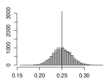
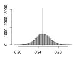
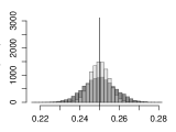
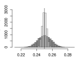
Figure 2: Histograms of the kernel smoothers (1) at the query $(x,x^{\prime})=(0.5,0.5)$. The bandwidth is set to $h=n^{-1/(s+d)}$ with respect to the number of nodes $n=500$. The black vertical line represents the true conditional expectation $f(0.5,0.5)=0.25$.

$s=0.75$	$s=1$	$s=2$	$s=3$

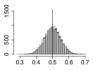
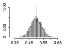
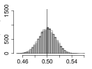
Figure 3: Histograms of the kernel smoother (3) at the query $x=0.5$. The bandwidth and the regularization parameter are $h=n^{-1/(s+d)}$, $\lambda_{n}=n^{-1/2}$, respectively, where $n=5000$ represents the number of covariates.

Herein, we present similar experiments for nonparametric regression. Given covariates $\{X_{i}\in\mathcal{X}:i=1,\ldots,n\}$, an outcome $Y_{i}\in\mathcal{Y}$ independently follows a conditional distribution $Q(Y_{i}\mid X_{i})$. For estimating the conditional mean $f(x):=\mathbb{E}[Y\mid X=x]$ at a query $x$, we define a kernel smoother

$$\widehat{f}_{n,h}(x):=\frac{n^{-1}\sum_{i=1}^{n}Y_{i}\{K_{h}(x-X_{i})+\lambda_{n}\}}{n^{-1}\sum_{i=1}^{n}\{K_{h}(x-X_{i})+\lambda_{n}\}}$$ (3)

similarly to the nonparametric link regression (1).

Using the function $f(x)=x$ and a query $x=0.5$, the histograms of the estimator (3) via $10^{4}$ times experiments are illustrated in the following Figure 3.

Appendix C Proofs of main results

Using supporting Lemmas (shown in Supplement C.1), this section provides the proofs of Theorem 2.1 (shown in Supplement C.2) and Theorem 2.3 (shown in Supplement C.3). For proofs, we employ the following symbols:

$$W_{i_{1},i_{2}}(x,x^{\prime};X) :=\frac{K_{h}(x-X_{i_{1}})K_{h}(x^{\prime}-X_{i_{2}})+\lambda_{n}}{\sum_{(i_{1},i_{2})\in I_{n}}\{K_{h}(x-X_{i_{1}})K_{h}(x^{\prime}-X_{i_{2}})+\lambda_{n}\}},$$

$$S_{n,h} :=|I_{n}|^{-1}\sum_{(i_{1},i_{2})\in I_{n}}\{f(X_{i_{1}},X_{i_{2}})-f(x,x^{\prime})\}\{K_{h}(x-X_{i_{1}})K_{h}(x^{\prime}-X_{i_{2}})+\lambda_{n}\},$$

$$T_{n,h} :=|I_{n}|^{-1}\sum_{(i_{1},i_{2})\in I_{n}}\{K_{h}(x-X_{i_{1}})K_{h}(x^{\prime}-X_{i_{2}})+\lambda_{n}\},$$

$$\overline{T}_{n,h} =\mathbb{E}(T_{n,h}),\quad\text{and }\varepsilon_{n,h}:=\frac{1}{T_{n,h}}-\frac{1}{\overline{T}_{n,h}}.$$

These satisfy

$$\widehat{f}_{n,h}(x,x^{\prime}) =\sum_{(i_{1},i_{2})\in I_{n}}Y_{i_{1}i_{2}}W_{i_{1},i_{2}}(x,x^{\prime};X),$$ (4)

$$\sum_{(i_{1},i_{2})\in I_{n}}W_{i_{1},i_{2}}(x,x^{\prime};X) =1,\text{ and }$$ (5)

$$\mathbb{E}(\widehat{f}_{n,h}(x,x^{\prime})\mid X)-f(x,x^{\prime}) =\frac{S_{n,h}}{T_{n,h}}.$$ (6)

C.1 Supporting lemmas

We begin with stating supporting lemmas used in the proofs of main results. Expression of variance of $U$-statistics (Lemma C.1); upper estimates of moments of the kernel (Lemma C.2); the Rosenthal inequality for $U$-statistics (Lemma C.3); the small ball estimate (Lemma C.4); a lower bound of the number of observed covariates in a ball (Lemma C.5); upper bounds of moments of $T_{n,h}$ (Lemma C.6); upper bounds of moments of $\varepsilon_{n,h}$ (Lemma C.7); An upper bound of the variance of $S_{n,h}$ (Lemma C.8); the fourth moment evaluation of $S_{n,h}$ (Lemma C.9).

For a bounded function $k:\mathcal{X}^{2}\to\mathbb{R}$ and an i.i.d. sequence $\{X_{1},\ldots,X_{n}\}$, let

$$U_{n}:=|I_{n}|^{-1}\sum_{(i_{1},i_{2})\in I_{n}}k(X_{i_{1}},X_{i_{2}})=\binom{n}{2}^{-1}\sum_{1\leq i_{1}<i_{2}\leq n}\left\{\frac{k(X_{i_{1}},X_{i_{2}})+k(X_{i_{2}},X_{i_{1}})}{2}\right\}.$$

From the symmetric expression of $U_{n}$ (the rightmost in the definition of $U_{n}$), we get the following expression on the variance of $U_{n}$.

Lemma C.1 (Lee,, 1990).

We have

$$\operatorname{Var}[U_{n}]=\frac{4(n-2)}{n(n-1)}\zeta_{1}+\frac{2}{n(n-1)}\zeta_{2},$$

where

$$\zeta_{1}:=\operatorname{Var}\left[\mathbb{E}\left[\frac{k(X,X^{\prime})+k(X^{\prime},X)}{2}\mid X\right]\right]\text{ and }\zeta_{2}:=\operatorname{Var}\left[\frac{k(X,X^{\prime})+k(X^{\prime},X)}{2}\right].$$

In addition, we get

$$\zeta_{1} \leq\frac{1}{2}\left[\operatorname{Var}[\mathbb{E}[k(X,X^{\prime})\mid X]]+\operatorname{Var}[\mathbb{E}[k(X^{\prime},X)\mid X]]\right],\text{ and }$$

$$\zeta_{2} \leq\operatorname{Var}[k(X,X^{\prime})].$$

We need an upper bound on the expectation of $K_{h}^{\alpha}(x-X)\|x-X\|^{\beta}$ for $\alpha,\beta\geq 0$. Let

$$\kappa_{\alpha,\beta}:=\|m\|_{\infty}\left\{\int_{\mathbb{R}^{d}}K(z)^{\alpha}\mathrm{d}z\right\}\left\{\sup_{z\,\in\,\text{supp}\,K}\|z\|^{\beta}\right\}\quad(\text{with }0^{0}=0\text{ for }\alpha=0),$$

which is bounded since $K$ is compactly supported. We obtain the following Lemma C.2.

Lemma C.2.

We have $\mathbb{E}[K_{h}(x-X)^{\alpha}\|x-X\|^{\beta}]\leq\kappa_{\alpha,\beta}h^{(1-\alpha)d+\beta}$ for any $\alpha,\beta\geq 0$.

Proof.

Letting $Z:=(x-X)/h$, we have

$$\mathbb{E}[K_{h}(x-X)^{\alpha}\|x-X\|^{\beta}] =\int_{\mathcal{X}}K_{h}(x-X)^{\alpha}\|x-X\|^{\beta}m(X)\mathrm{d}X$$

$$=\int\{h^{-d}K(Z)\}^{\alpha}\|hZ\|^{\beta}m(x+hZ)h^{d}\mathrm{d}Z$$

$$\leq\|m\|_{\infty}\left\{\int K(Z)^{\alpha}\mathrm{d}Z\right\}\left\{\sup_{Z\,\in\,\text{supp}\,K}\|Z\|^{\beta}\right\}h^{(1-\alpha)d+\beta}$$

$$=\kappa_{\alpha,\beta}h^{(1-\alpha)d+\beta}.$$

∎

We use the following Rosenthal type estimate of the fourth moment of $U$-statistics.

Lemma C.3.

There exists an absolute constant $C_{R}>0$ for which we have

$$\mathbb{E}\left[\left(\sum_{(i_{1},i_{2})\in I_{n}}k(X_{i_{1}},X_{i_{2}})\right)^{4}\right]$$

$$\leq C_{R}\Bigg{\{}\Bigg{(}\sum_{(i_{1},i_{2})\in I_{n}}\mathbb{E}[k(X^{(1)}_{i_{1}},X^{(2)}_{i_{2}})]\Bigg{)}^{4}+\sum_{1\leq i_{1}\leq n}\mathbb{E}\left[\Bigg{(}\sum_{1\leq i_{2}\leq n}\mathbb{E}[k(X_{i_{1}}^{(1)},X_{i_{2}}^{(2)})\mid X_{i_{1}}^{(1)}]\Bigg{)}^{4}\right]$$

$$\quad\quad\quad+\sum_{1\leq i_{2}\leq n}\mathbb{E}\left[\Bigg{(}\sum_{1\leq i_{1}\leq n}\mathbb{E}[k(X_{i_{1}}^{(1)},X_{i_{2}}^{(2)})\mid X_{i_{2}}^{(2)}]\Bigg{)}^{4}\right]+\sum_{(i_{1},i_{2})\in I_{n}}\mathbb{E}[\{k(X^{(1)}_{i_{1}},X^{(2)}_{i_{2}})\}^{4}]\Bigg{\}}.$$

Proof.

Combining the decoupling inequality in de la Pena and Montgomery-Smith, (1995) and the Rosenthal inequality (2.2”) in Giné et al., (2000) gives the desired inequality. ∎

We also use the following lower estimate of a small ball probability.

Lemma C.4.

Let $X$ be a random vector from a density $m$ satisfying Condition 2.3 (b). For any $x_{0}\in\mathcal{X}$ and any $h>0$, we have

$$\mathbb{P}(\|X-x_{0}\|\leq h) \geq\frac{lr^{d}\pi^{d/2}}{\Gamma(d/2+1)}h^{d}=:C_{B}h^{d},$$

$$\mathbb{P}(\|X-x_{0}\|\leq h) \leq\frac{ur^{d}\pi^{d/2}}{\Gamma(d/2+1)}h^{d}=:C^{\prime}_{B}h^{d},$$

where $\Gamma(x)$ is the Gamma function.

The proof is easy and omitted.

In the following, the number of observed covariates considered in the nonparametric link regression is evaluated.

Lemma C.5.

Under the condition 2.3 (a) with $n^{-1/d}\leq h\leq 1$, there exists $C_{K}>0$ independent of $n,h$ such that

$$\frac{1}{|I_{n}|}\sum_{(i_{1},i_{2})\in I_{n}}K_{h}(x-X_{i_{1}})K_{h}(x^{\prime}-X_{i_{2}})\geq C_{K}.$$

Proof.

Let $r:=\sup\{\|x\|_{2}\mid K(x)>0\}$, and let

$$\mathcal{P}_{n,h}(x):=\left\{i\in[n]\mid\left\|\frac{x-X_{i}}{h}\right\|\leq r\right\};$$

together with the inequality $\max_{i}\min_{j}\|X_{i}-X_{j}\|\leq C_{X}/n^{1/d}$, its cardinality is lower-bounded by

$$|\mathcal{P}_{n,h}(x)| \geq\Bigg{|}\left\{t=(t_{1},t_{2},\ldots,t_{d})\in\mathbb{Z}^{d}\setminus\{\mathbf{0}\}\,\mid\,\left\|\frac{(C_{X}/n^{1/d})t}{h}\right\|\leq r\right\}\Bigg{|}$$

$$\geq\Bigg{|}\left\{t=(t_{1},t_{2},\ldots,t_{d})\in\mathbb{Z}^{d}\setminus\{\mathbf{0}\}\,\mid\,\left\|t\right\|\leq\frac{r}{C_{X}}n^{1/d}h\right\}\Bigg{|}$$

$$\geq C^{\prime}(hn^{1/d})^{d}\geq C^{\prime}nh^{d}$$

for some $C^{\prime}>0$. Therefore, we get

$$|I_{n}|^{-1}\sum_{(i_{1},i_{2})\in I_{n}} K_{h}(x-X_{i_{1}})K_{h}(x^{\prime}-X_{i_{2}})$$

$$=|I_{n}|^{-1}\sum_{(i_{1},i_{2})\in I_{n}\cap\{P_{n,h}(x)\times P_{n,h}(x^{\prime})\}}K_{h}(x-X_{i_{1}})K_{h}(x^{\prime}-X_{i_{2}})$$

$$=|I_{n}|^{-1}\sum_{(i_{1},i_{2})\in I_{n}\cap\{P_{n,h}(x)\times P_{n,h}(x^{\prime})\}}h^{-d}K\left(\frac{x-X_{i_{1}}}{h}\right)h^{-d}K\left(\frac{x^{\prime}-X_{i_{2}}}{h}\right)$$

$$=\frac{|I_{n}\cap\{P_{n,h}(x)\times P_{n,h}(x^{\prime})\}|}{|I_{n}|}h^{-2d}(\underline{k}K_{\max})^{2}$$

$$\geq\frac{\min\left\{\binom{|\mathcal{P}_{n,h}(x)|}{2},\binom{|\mathcal{P}_{n,h}(x^{\prime})|}{2}\right\}}{\binom{n}{2}}h^{-2d}(\underline{k}K_{\max})^{2}$$

$$\geq C^{\prime\prime}\frac{(C^{\prime}nh^{d})^{2}}{n^{2}}h^{-2d}(\underline{k}K_{\max})^{2}\quad\text{for some }\,C^{\prime\prime}$$

$$=C^{\prime\prime}(C^{\prime}\underline{k}K_{\max})^{2}=:C_{K},$$

which proves the assertion. ∎

The $q$-th moment of $T_{n,h}$ is evaluated as follows.

Lemma C.6.

Let $q\in\mathbb{N}$. Provided that $h\leq 1$, there exist $C_{T,1},C_{T,2}\geq 0$ independent of $n$ and $h$ such that

$$\mathbb{E}(|T_{n,h}-\overline{T}_{n,h}|^{q})\leq C_{T,1}/(nh^{d})^{q}+C_{T,2}/(nh^{d})^{2q-2}.$$

Proof.

With $\mathbb{E}(K_{h}(x-X))=\kappa_{1,0}=O(1)$ and $k(X,X^{\prime}):=K_{h}(x-X)K_{h}(x^{\prime}-X^{\prime})-\kappa_{1,0}^{2}$ satisfying

$$T_{n,h}-\overline{T}_{n,h}=|I_{n}|^{-1}\sum_{(i_{1},i_{2})\in I_{n}}k(X_{i_{1}},X_{i_{2}})\quad\text{and}\quad\mathbb{E}(k(X,X^{\prime}))=0,$$

we have

$$\mathbb{E}(|k(X,X^{\prime})|^{q}) =\mathbb{E}\left(\sum_{j=0}^{q}(-1)^{j}\binom{q}{j}K_{h}(x-X)^{j}K_{h}(x^{\prime}-X^{\prime})^{j}(\kappa_{1,0}^{2})^{q-j}\right)$$

$$\leq\sum_{j=0}^{q}\binom{q}{j}\kappa_{1,0}^{2(q-j)}\mathbb{E}(K_{h}(x-X)^{j})\mathbb{E}(K_{h}(x^{\prime}-X^{\prime})^{j})$$

$$\leq\sum_{j=0}^{q}\binom{q}{j}\kappa_{1,0}^{2(q-j)}\kappa_{j,0}h^{-d(j-1)}\kappa_{j,0}h^{-d(j-1)}$$

$$=\left\{1+\sum_{j=0}^{q-1}\binom{q}{j}\kappa_{1,0}^{2(q-j)}\kappa_{j,0}^{2}h^{2d(q-j)}\right\}h^{-2d(q-1)}$$

$$\leq C_{T}^{\prime}h^{-2d(q-1)},$$

with $C_{T}^{\prime}:=1+(q-1)\max_{j}\{\binom{q}{j}\kappa_{1,0}^{2(q-j)}\kappa_{j,0}^{2}\}$. Applying Lemma 2.1 of Fu, (2011) to $k(X,X^{\prime})$ yields

$$\mathbb{E}(|T_{n,h}-\overline{T}_{n,h}|^{q}) \leq C_{T,1}^{\prime}n^{-q}\mathbb{E}(|k(X,X^{\prime})|^{2})^{q/2}+C_{T,2}^{\prime}n^{2-2q}\mathbb{E}(|k(X,X^{\prime})|^{q})$$

$$\leq C_{T,1}n^{-q}(h^{-2d(2-1)})^{q/2}+C_{T,2}n^{2-2q}h^{-2d(q-1)}$$

$$=C_{T,1}/(nh^{d})^{q}+C_{T,2}/(nh^{d})^{2q-2}.$$

∎

The $q$-th moment of $\varepsilon_{n,h}$ is also evaluated as follows.

Lemma C.7.

Let $q\in\mathbb{N}$. Provided that $h\leq 1$ and $1/\{\lambda_{n}(nh^{d})^{\nu}\}\leq 1$ for some $\nu>0$, there exist $C_{\varepsilon,1},C_{\varepsilon,2}>0$ independent of $n$ and $h$ such that

$$\mathbb{E}(|\varepsilon_{n,h}|^{q})\leq C_{\varepsilon,1}/(nh^{d})^{q}+C_{\varepsilon,2}/(nh^{d})^{2q-2}.$$

Proof.

$\overline{T}_{n,h}\geq l^{2}+\lambda_{n}$ indicate that

$$\mathbb{E}(|\varepsilon_{n,h}|^{q}) =\mathbb{E}\bigg{[}\frac{|T_{n,h}-\overline{T}_{n,h}|^{q}}{\overline{T}_{n,h}^{q}T_{n,h}^{q}}\bigg{]}$$

$$=\mathbb{E}\bigg{[}\frac{|T_{n,h}-\overline{T}_{n,h}|^{q}}{\overline{T}_{n,h}^{q}T_{n,h}^{q}}\mathbbm{1}\left(|T_{n,h}-\overline{T}_{n,h}|\leq\frac{\overline{T}_{n,h}}{2}\right)\bigg{]}$$

$$\hskip 60.00009pt+\mathbb{E}\bigg{[}\frac{|T_{n,h}-\overline{T}_{n,h}|^{q}}{\overline{T}_{n,h}^{q}T_{n,h}^{q}}\mathbbm{1}\left(|T_{n,h}-\overline{T}_{n,h}|>\frac{\overline{T}_{n,h}}{2}\right)\bigg{]}$$

$$\leq\frac{1}{(l^{2})^{q}(l^{2}/2)^{q}}\mathbb{E}\bigg{[}|T_{n,h}-\overline{T}_{n,h}|^{q}\bigg{]}+\frac{1}{(l^{2})^{q}\lambda_{n}^{q}}\mathbb{E}\bigg{[}|T_{n,h}-\overline{T}_{n,h}|^{q}\mathbbm{1}\left(|T_{n,h}-\overline{T}_{n,h}|>\frac{\overline{T}_{n,h}}{2}\right)\bigg{]}.$$ (7)

Further, for any $\nu>0$, we have

$$\eqref{eq:epsilon_eq1} \leq\frac{2^{q}}{l^{4q}}\mathbb{E}\bigg{[}|T_{n,h}-\overline{T}_{n,h}|^{q}\bigg{]}+\frac{1}{l^{2q}\lambda_{n}^{q}}\mathbb{E}\bigg{[}\frac{|T_{n,h}-\overline{T}_{n,h}|^{\nu}}{|T_{n,h}-\overline{T}_{n,h}|^{\nu}}|T_{n,h}-\overline{T}_{n,h}|^{q}\mathbbm{1}\left(|T_{n,h}-\overline{T}_{n,h}|>\frac{\overline{T}_{n,h}}{2}\right)\bigg{]}$$

$$\leq\frac{2^{q}}{l^{4q}}\mathbb{E}\bigg{[}\left\{T_{n,h}-\overline{T}_{n,h}\right\}^{q}\bigg{]}+\frac{2^{\nu}}{l^{2q+2\nu}\lambda_{n}^{q}}\mathbb{E}\bigg{[}(T_{n,h}-\overline{T}_{n,h})^{q+\nu}\bigg{]}.$$ (8)

Therefore, by specifying sufficiently large $\nu=\nu(q)$ satisfying $\lambda_{n}^{q}(nh^{d})^{\nu}\geq 1$, Lemma C.6 ensures the existence of $C_{\varepsilon,1}^{\prime},C_{\varepsilon,2}^{\prime},C_{\varepsilon,3}^{\prime},C_{\varepsilon,4}^{\prime}>0$ such that

$$\eqref{eq:epsilon_eq2} \leq C_{\varepsilon,1}^{\prime}/(nh^{d})^{q}+C_{\varepsilon,2}^{\prime}/(nh^{d})^{2q-2}+C_{\varepsilon,3}^{\prime}/\{\lambda_{n}^{q}(nh^{d})^{q+\nu}\}+C_{\varepsilon,4}^{\prime}/\{\lambda_{n}^{q}(nh^{d})^{2q+2\nu-2}\}$$

$$\leq C_{\varepsilon,1}/(nh^{d})^{q}+C_{\varepsilon,2}/(nh^{d})^{2q-2},$$

which proves the assertion.

∎

The variance of $S_{n,h}$ is evaluated as follows.

Lemma C.8.

Provided that $n^{-1/d}\leq h\leq 1$ and $\lambda_{n}\leq h^{d}$, there exists $C_{V,S}>0$ independent of $n$ and $h$ such that $\operatorname{Var}[S_{n,h}]\leq C_{V,S}h^{2\beta}(nh^{d})^{-1}$.

Proof.

To evaluate the variance of $S_{n,h}$, we apply Lemma C.1 to

$$k(X,X^{\prime}) =\{f(X,X^{\prime})-f(x,x^{\prime})\}\{K_{h}(x-X)K_{h}(x^{\prime}-X^{\prime})+\lambda_{n}\}$$

and bound $\zeta_{1},\zeta_{2}$ therein as follows.

Step A: Bounding $\zeta_{1}$. Letting $k^{(1)}(X):=\mathbb{E}[k(X,X^{\prime})\mid X]$ and $k^{(2)}(X):=\mathbb{E}[k(X^{\prime},X)\mid X]$, we have

$$\zeta_{1}\leq\frac{1}{2}\left(\operatorname{Var}[k^{(1)}(X)]+\operatorname{Var}[k^{(2)}(X)]\right)\leq\frac{1}{2}\left(\mathbb{E}[\{k^{(1)}(X)\}^{2}]+\mathbb{E}[\{k^{(2)}(X)\}^{2}]\right).$$

By the inequality

$$|f(X,X^{\prime})-f(x,x^{\prime})| \leq|f(X,X^{\prime})-f(x,X^{\prime})|+|f(x,X^{\prime})-f(x,x^{\prime})|$$

$$\leq L\|x-X\|^{\beta}+L\|x^{\prime}-X^{\prime}\|^{\beta},$$

we get the following bound on $k^{(1)}(X)$:

$$|k^{(1)}(X)| \leq\mathbb{E}\left[|f(X,X^{\prime})-f(x,x^{\prime})|\{K_{h}(x-X)K_{h}(x^{\prime}-X^{\prime})+\lambda_{n}\}\mid X\right]$$

$$\leq L\mathbb{E}\left[K_{h}(x-X)K_{h}(x^{\prime}-X^{\prime})\{\|x-X\|^{\beta}+\|x^{\prime}-X^{\prime}\|^{\beta}\}\mid X\right]$$

$$\hskip 10.00002pt+L\lambda_{n}\mathbb{E}\left[\{\|x-X\|^{\beta}+\|x^{\prime}-X^{\prime}\|^{\beta}\}\mid X\right].$$

By Lemma C.2, this is further bounded from above as follows:

$$|k^{(1)}(X)| \leq L\{\tau_{1}+\tau_{2}+\tau_{3}+\tau_{4}\},$$

where

$$\tau_{1} :=\kappa_{1,0}K_{h}(x-X)\|x-X\|^{\beta}, \tau_{2} :=\kappa_{1,\beta}K_{h}(x-X)h^{\beta},$$

$$\tau_{3} :=\lambda_{n}\|x-X\|^{\beta}, \tau_{4} :=\lambda_{n}\kappa_{0,\beta}h^{\beta}.$$

Then we get

$$\mathbb{E}[\{k^{(1)}(x,X)\}^{2}]\leq L^{2}\sum_{j_{1}=1}^{4}\sum_{j_{2}=1}^{4}\mathbb{E}[\tau_{j_{1}}\tau_{j_{2}}].$$

Here by Lemma C.2, we bound the diagonal components $\{\mathbb{E}[\tau_{i}^{2}]:i=1,\ldots,4\}$ as

$$\mathbb{E}[\tau_{1}^{2}] =\kappa_{1,0}^{2}\mathbb{E}[K_{h}(x-X)^{2}\|x-X\|^{2\beta}] \leq \kappa_{1,0}^{2}\kappa_{2,2\beta}\,\,(h^{-d+2\beta}) = O(h^{-d+2\beta}),$$

$$\mathbb{E}[\tau_{2}^{2}] =\kappa_{1,\beta}^{2}\mathbb{E}[K_{h}(x-X)^{2}]\,\,h^{2\beta} \leq \kappa_{1,\beta}^{2}\kappa_{2,0}\,\,(h^{-d+2\beta}) = O(h^{-d+2\beta}),$$

$$\mathbb{E}[\tau_{3}^{2}] =\lambda_{n}^{2}\,\,\mathbb{E}[K_{h}(x-X)^{0}\|x-X\|^{2\beta}] \leq \kappa_{0,2\beta}\,\,(\lambda_{n}^{2}h^{d+2\beta}) = O(\lambda_{n}^{2}h^{d+2\beta}),$$

$$\mathbb{E}[\tau_{4}^{2}] =\lambda_{n}^{2}\,\,\kappa_{0,\beta}^{2}\,\,h^{2\beta} \leq \kappa_{0,\beta}^{2}\,\,(\lambda_{n}^{2}h^{d+2\beta}) = O(\lambda_{n}^{2}h^{d+2\beta}).$$

Similarly, we bound the off-diagonal components $\{\mathbb{E}[\tau_{i}\tau_{j}]:1\leq i<j\leq 4\}$ as

$$\mathbb{E}[\tau_{1}\tau_{2}] =\kappa_{1,0}\kappa_{1,\beta}\mathbb{E}[K_{h}(x-X)^{2}\|x-X\|^{\beta}]\,\,h^{\beta} \leq \kappa_{1,0}\kappa_{1,\beta}\kappa_{2,\beta}\,\,(h^{-d+2\beta}) = O(h^{-d+2\beta}),$$

$$\mathbb{E}[\tau_{1}\tau_{3}] =\lambda_{n}\,\,\kappa_{1,0}\mathbb{E}[K_{h}(x-X)\|x-X\|^{2\beta}] \leq \kappa_{1,0}\kappa_{1,2\beta}\,\,(\lambda_{n}h^{2\beta}) = O(\lambda_{n}h^{2\beta}),$$

$$\mathbb{E}[\tau_{1}\tau_{4}] =\lambda_{n}\,\,\kappa_{1,0}\kappa_{0,\beta}\mathbb{E}[K_{h}(x-X)\|x-X\|^{\beta}]\,\,h^{\beta} \leq \kappa_{1,0}\kappa_{0,\beta}\kappa_{1,\beta}\,\,(\lambda_{n}h^{2\beta}) = O(\lambda_{n}h^{2\beta}),$$

$$\mathbb{E}[\tau_{2}\tau_{3}] =\lambda_{n}\,\,\kappa_{1,\beta}\mathbb{E}[K_{h}(x-X)\|x-X\|^{\beta}]\,\,h^{\beta} \leq \kappa_{1,\beta}\kappa_{1,\beta}\,\,(\lambda_{n}h^{2\beta}) = O(\lambda_{n}h^{2\beta}),$$

$$\mathbb{E}[\tau_{2}\tau_{4}] =\lambda_{n}\,\,\kappa_{1,\beta}\kappa_{0,\beta}\mathbb{E}[K_{h}(x-X)]\,\,h^{2\beta} \leq \kappa_{1,\beta}\kappa_{0,\beta}\kappa_{1,0}\,\,(\lambda_{n}h^{2\beta}) = O(\lambda_{n}h^{2\beta}),$$

$$\mathbb{E}[\tau_{3}\tau_{4}] =\lambda_{n}^{2}\,\,\kappa_{0,\beta}\mathbb{E}[K_{h}(x-X)^{0}\|x-X\|^{\beta}]\,\,h^{\beta} \leq \kappa_{0,\beta}\kappa_{0,\beta}\,\,(\lambda_{n}^{2}h^{d+2\beta}) = O(\lambda_{n}^{2}h^{d+2\beta}).$$

These inequalities indicate that there exist positive constants $D_{1},D_{2},D_{3}$ depending only on $\{\kappa_{i,j\beta}:i=0,1,j=0,1,2\}$ for which we have

$$\mathbb{E}[\{k^{(1)}(x,X)\}^{2}] \leq L^{2}\{D_{1}h^{-d+2\beta}+D_{2}\lambda_{n}h^{2\beta}+D_{3}\lambda_{n}^{2}h^{d+2\beta}\}$$

$$\leq L^{2}h^{-d+2\beta}\{D_{1}+D_{2}\lambda_{n}h^{d}+D_{3}\lambda_{n}^{2}h^{2d}\}$$

$$\leq Dh^{-d+2\beta}\text{ with $D=L^{2}(D_{1}+D_{2}+D_{3})$},$$

where we use $\lambda_{n}\leq h^{d}$ and $h\leq 1$. Similarly, there exists a positive constant $D^{\prime}$ depending only on $L$ and $\{\kappa_{i,j\beta}:i=0,1,j=0,1,2\}$ for which we have

$$\mathbb{E}[\{k^{(2)}(x,X)\}^{2}]\leq D^{\prime}h^{-d+2\beta}.$$

Consequently, we obtain

$$\zeta_{1} \leq\frac{1}{2}\left\{\mathbb{E}[\{k^{(1)}(x,X)\}^{2}]+\mathbb{E}[\{k^{(2)}(x,X)\}^{2}]\right\}=\frac{D+D^{\prime}}{2}\,\,h^{-d+2\beta}.$$ (9)

Step B: Bounding $\zeta_{2}$. By the Hölder continuity of $f$, we have

$$\zeta_{2}\leq\operatorname{Var}[k(X,X^{\prime})] \leq\mathbb{E}[k(X,X^{\prime})^{2}]$$

$$\leq\mathbb{E}\left[\{K_{h}(x-X)K_{h}(x^{\prime}-X^{\prime})+\lambda_{n}\}^{2}|f(X,X^{\prime})-f(x,x^{\prime})|^{2}\right]$$

$$\leq\mathbb{E}\left[\{K_{h}(x-X)K_{h}(x^{\prime}-X^{\prime})+\lambda_{n}\}^{2}\{L\|x-X\|^{\beta}+L\|x^{\prime}-X^{\prime}\|^{\beta}\}^{2}\right]$$

$$\leq L^{2}\sum_{j_{1}=0}^{2}\sum_{j_{2}=0}^{2}\binom{2}{j_{1}}\binom{2}{j_{2}}\xi_{j_{1},j_{2}},$$

where

$$\xi_{k,l} :=\mathbb{E}[\{K_{h}(x-X)K_{h}(x^{\prime}-X^{\prime})\}^{j_{1}}\lambda_{n}^{2-j_{1}}\|x-X\|^{j_{2}\beta}\|x^{\prime}-X^{\prime}\|^{(2-j_{2})\beta}].$$

Here Lemma C.2 gives

$$\xi_{k,l} =\lambda_{n}^{2-j_{1}}\mathbb{E}[K_{h}(x-X)^{j_{1}}\|x-X\|^{j_{2}\beta}]\mathbb{E}[K_{h}(x^{\prime}-X^{\prime})^{j_{1}}\|x^{\prime}-X^{\prime}\|^{(2-j_{2})\beta}]$$

$$\leq\lambda_{n}^{2-j_{1}}\,\,\kappa_{j_{1},j_{2}\beta}\kappa_{j_{1},(2-j_{2})\beta}\,\,h^{(1-j_{1})d+j_{2}\beta}h^{(1-j_{1})d+(2-j_{2})\beta}$$

$$=\kappa_{j_{1},j_{2}\beta}\kappa_{j_{1},(2-j_{2})\beta}\lambda_{n}^{2-j_{1}}h^{2(1-j_{1})d+2\beta}$$

$$\leq D_{4}\,\,h^{-2d+2\beta},$$

where $D_{4}$ is a positive constant depending only on $\{\kappa_{j_{1},j_{2}\beta}:j_{1}=0,1,2,j_{2}=0,1,2\}$. This concludes that there exists a positive constant depending only on $L$ and $\{\kappa_{j_{1},j_{2}\beta}:j_{1}=0,1,2,j_{2}$ for which we have

$$\zeta_{2}\leq D^{\prime\prime}h^{-2d+2\beta}.$$ (10)

Final step: Combining bounds on $\zeta_{1}$ and $\zeta_{2}$. Combining (9) and (10) yields

$$\operatorname{Var}[S_{n,h}] =\frac{4(n-2)}{n(n-1)}\zeta_{1}+\frac{2}{n(n-1)}\zeta_{2} \leq 2(D+D^{\prime})h^{2\beta}(nh^{d})^{-1}\,\,+\,\,4D^{\prime\prime}h^{2\beta}(nh^{d})^{-2}$$

$$\leq (2D+2D^{\prime}+4D^{\prime\prime})h^{2\beta}(nh^{d})^{-1}(1+(nh^{d})^{-1})$$

which completes the proof. ∎

We last evaluate the fourth moment of $S_{n,h}$ as follows.

Lemma C.9.

Provided that $n^{-1/d}\leq h\leq 1$, there exists $C_{E,S}>0$ independent of $n$ and $h$ such that $\mathbb{E}(S_{n,h}^{4})\leq C_{E,S}h^{4\beta}$.

Proof of Lemma C.9.

To evaluate $b_{n}:=\mathbb{E}(S_{n,h}^{4})$, we prepare the multi-index notation: let

$$\mathcal{J}_{k}(m):=\{(j_{1},j_{2},\ldots,j_{k})\in\{0,1,2,\ldots,m\}\mid j_{1}+j_{2}+\cdots+j_{k}=m\},$$

and let

$$\binom{m}{j_{1},j_{2},\ldots,j_{k}}=\frac{m!}{j_{1}!j_{2}!\cdots j_{k}!}.$$

Let

$$h_{i_{1},i_{2}}(X,X^{\prime}):=\{\|x-X\|^{\beta}+\|x^{\prime}-X^{\prime}\|^{\beta}\}\{K_{h}(x-X)K_{h}(x^{\prime}-X^{\prime})+\lambda_{n}\}$$

and let $X^{(1)}$ and $X^{(2)}$ be independent copies of $X$. By the inequality $|f(X,X^{\prime})-f(x,x^{\prime})|\leq L\|x-X\|^{\beta}+L\|x^{\prime}-X^{\prime}\|^{\beta}$ and by Lemma C.3, we get

$$b_{n} =\frac{1}{|I_{n}|^{4}}\mathbb{E}\Bigg{[}\Bigg{(}\sum_{(i_{1},i_{2})\in I_{n}}|f(X_{i_{1}},X_{i_{2}})-f(x,x^{\prime})|\{K_{h}(x-X_{i_{1}})K_{h}(x^{\prime}-X_{i_{2}})+\lambda_{n}\}\Bigg{)}^{4}\Bigg{]}$$

$$\leq\frac{L^{4}}{|I_{n}|^{4}}\mathbb{E}\Bigg{[}\Bigg{(}\sum_{(i_{1},i_{2})\in I_{n}}h_{i_{1},i_{2}}(X_{i_{1}},X_{i_{2}})\Bigg{)}^{4}\Bigg{]}$$

$$\leq\frac{C_{R}L^{4}}{|I_{n}|^{4}}\Bigg{\{}\underbrace{\Bigg{(}\sum_{(i_{1},i_{2})\in I_{n}}\mathbb{E}\left[h_{i_{1},i_{2}}(X^{(1)}_{i_{1}},X^{(2)}_{i_{2}})\right]\Bigg{)}^{4}}_{=:E_{1}}$$

$$\hskip 40.00006pt+\underbrace{\sum_{1\leq i_{1}\leq n}\mathbb{E}\Bigg{[}\Bigg{(}\sum_{1\leq i_{2}\leq n}\mathbb{E}[h_{i_{1},i_{2}}(X^{(1)}_{i_{1}},X^{(2)}_{i_{2}})\mid X^{(1)}_{i_{1}}]\Bigg{)}^{4}\Bigg{]}}_{=:E_{2}}$$

$$\hskip 40.00006pt+\underbrace{\sum_{1\leq i_{2}\leq n}\mathbb{E}\Bigg{[}\Bigg{(}\sum_{1\leq i_{1}\leq n}\mathbb{E}[h_{i_{1},i_{2}}(X^{(1)}_{i_{1}},X^{(2)}_{i_{2}})\mid X^{(2)}_{i_{2}}]\Bigg{)}^{4}\Bigg{]}}_{=:E_{3}}+\underbrace{\sum_{(i_{1},i_{2})\in I_{n}}\mathbb{E}\Bigg{[}h_{i_{1},i_{2}}^{4}(X^{(1)}_{i_{1}},X^{(2)}_{i_{2}})\Bigg{]}}_{=:E_{4}}\Bigg{\}}.$$

We bound $E_{1}$, by using the identity

$$\mathbb{E}\big{[}h_{i_{1},i_{2}}(X^{(1)}_{i_{1}},X^{(2)}_{i_{2}})\big{]} =\mathbb{E}\big{[}K_{h}(x-X_{i_{1}}^{(1)})\|x-X_{i_{1}}^{(1)}\|^{\beta}\big{]}\,\mathbb{E}\big{[}K_{h}(x^{\prime}-X_{i_{2}}^{(2)})\|x^{\prime}-X_{i_{2}}^{(2)}\|^{0}\big{]}$$

$$\quad+\mathbb{E}\big{[}K_{h}(x-X_{i_{1}}^{(1)})\|x-X_{i_{1}}^{(1)}\|^{0}\big{]}\,\mathbb{E}\big{[}K_{h}(x^{\prime}-X_{i_{2}}^{(2)})\|x^{\prime}-X_{i_{2}}^{(2)}\|^{\beta}\big{]}$$

$$\quad+\lambda_{n}\mathbb{E}\big{[}K_{h}(x-X_{i_{1}}^{(1)})^{0}\|x-X_{i_{1}}^{(1)}\|^{\beta}\big{]}+\lambda_{n}\mathbb{E}\big{[}K_{h}(x^{\prime}-X_{i_{2}}^{(2)})^{0}\|x^{\prime}-X_{i_{2}}^{(2)}\|^{\beta}\big{]}$$

and using Lemma C.2, as

$$E_{1}^{1/4} \leq\sum_{(i_{1},i_{2})\in I_{n}}\bigg{(}\kappa_{1,\beta}\kappa_{1,0}\,\,h^{\beta}+\kappa_{1,0}\kappa_{1,\beta}\,\,h^{\beta}+\kappa_{0,\beta}\,\,\lambda_{n}h^{d+\beta}+\kappa_{0,\beta}\,\,\lambda_{n}h^{d+\beta}\bigg{)}$$

$$=\sum_{(i_{1},i_{2})\in I_{n}}\bigg{(}2\kappa_{1,\beta}\kappa_{1,0}\,\,h^{\beta}+2\kappa_{0,\beta}\,\,\lambda_{n}h^{d+\beta}\bigg{)}$$

$$=n(n-1)\bigg{(}2\kappa_{1,\beta}\kappa_{1,0}h^{\beta}+2\lambda_{n}\kappa_{0,\beta}h^{d+\beta}\bigg{)}$$

$$=F_{1}\,\,n^{2}h^{\beta}\text{ with $F_{1}:=2(\kappa_{1,\beta}\kappa_{1,0}+\kappa_{0,\beta})$},$$

which implies

$$E_{1}\leq F_{1}^{4}\,\,n^{8}h^{4\beta}.$$ (11)

We bound $E_{2}$, by using the inequality

$$\mathbb{E} [h_{i_{1},i_{2}}(X^{(1)}_{i_{1}},X^{(2)}_{i_{2}})\mid X^{(1)}_{i_{1}}]$$

$$=\|x-X_{i_{1}}^{(1)}\|^{\beta}K_{h}(x-X_{i_{1}}^{(1)})\mathbb{E}\big{[}K_{h}(x^{\prime}-X_{i_{2}}^{(2)})\big{]} + K_{h}(x-X_{i_{1}}^{(1)})\mathbb{E}\big{[}K_{h}(x^{\prime}-X_{i_{2}}^{(2)})\|x^{\prime}-X_{i_{2}}^{(2)}\|^{\beta}\big{]}$$

$$\hskip 10.00002pt+\lambda_{n}\|x-X_{i_{1}}^{(1)}\|^{\beta} + \lambda_{n}\mathbb{E}\big{[}K_{h}(x^{\prime}-X_{i_{2}}^{(2)})^{0}\|x^{\prime}-X_{i_{2}}^{(2)}\|^{\beta}\big{]}$$

$$\leq\kappa_{1,0}\,\,\|x-X_{i_{1}}^{(1)}\|^{\beta}K_{h}(x-X_{i_{1}}^{(1)}) + \kappa_{1,\beta}\,\,h^{\beta}\,\,K_{h}(x-X_{i_{1}}^{(1)})$$

$$\hskip 10.00002pt+\lambda_{n}\|x-X_{i_{1}}^{(1)}\|^{\beta} + \lambda_{n}\,\,\kappa_{0,\beta}\,\,h^{d+\beta},$$

as

$$E_{2} \leq n^{4}\sum_{1\leq i_{1}\leq n}\mathbb{E}\Bigg{[}\Bigg{(}\kappa_{1,0}\,\,\|x-X_{i_{1}}^{(1)}\|^{\beta}K_{h}(x-X_{i_{1}}^{(1)})+\kappa_{1,\beta}\,\,h^{\beta}\,\,K_{h}(x-X_{i_{1}}^{(1)})$$

$$\hskip 160.00024pt+\lambda_{n}\|x-X_{i_{1}}^{(1)}\|^{\beta}+\lambda_{n}\,\,\kappa_{0,\beta}\,\,h^{d+\beta}\big{]}\Bigg{)}^{4}\Bigg{]}$$

$$=n^{4}\sum_{1\leq i_{1}\leq n}\sum_{(j_{1},j_{2},j_{3},j_{4})\in\mathcal{J}_{4}(4)}\binom{4}{j_{1},j_{2},j_{3},j_{4}}\mathcal{K}_{j_{1},j_{2},j_{3},j_{4}},$$

where

$$\mathcal{K}_{j_{1},j_{2},j_{3},j_{4}} :=\mathbb{E}\bigg{[}\bigg{\{}\|x-X_{i_{1}}^{(1)}\|^{\beta}K_{h}(x-X_{i_{1}}^{(1)})\kappa_{1,0}\bigg{\}}^{j_{1}}\bigg{\{}K_{h}(x-X_{i_{1}}^{(1)})\kappa_{1,\beta}h^{\beta}\bigg{\}}^{j_{2}}$$

$$\hskip 120.00018pt\cdot\bigg{\{}\lambda_{n}\|x-X_{i_{1}}^{(1)}\|^{\beta}\bigg{\}}^{j_{3}}\bigg{\{}\lambda_{n}\kappa_{0,\beta}h^{d+\beta}\bigg{\}}^{j_{4}}\bigg{]}.$$

Since we have

$$\mathcal{K}_{j_{1},j_{2},j_{3},j_{4}} =\kappa_{1,0}^{j_{1}}\kappa_{1,\beta}^{j_{2}}\kappa_{0,\beta}^{j_{4}}\,\,\mathbb{E}\bigg{[}K_{h}(x-X_{i_{1}}^{(1)})^{j_{1}+j_{2}}|x-X_{i_{1}}^{(1)}|^{(j_{1}+j_{3})\beta}\bigg{]}\,\,\lambda_{n}^{j_{3}+j_{4}}h^{j_{2}\beta+j_{4}(d+\beta)}$$

$$\leq\kappa_{1,0}^{j_{1}}\kappa_{1,\beta}^{j_{2}}\kappa_{0,\beta}^{j_{4}}\kappa_{j_{1}+j_{2},(j_{1}+j_{3})\beta}\,\,\lambda_{n}^{j_{3}+j_{4}}h^{(1-j_{1}-j_{2})d+(j_{1}+j_{3})\beta+j_{2}\beta+j_{4}(d+\beta)}$$

$$=\kappa_{1,0}^{j_{1}}\kappa_{1,\beta}^{j_{2}}\kappa_{0,\beta}^{j_{4}}\kappa_{j_{1}+j_{2},(j_{1}+j_{3})\beta}\,\,\lambda_{n}^{j_{3}+j_{4}}h^{(1-j_{1}-j_{2}+j_{4})d+(j_{1}+j_{2}+j_{3}+j_{4})\beta},$$

we further bound $E_{2}$ as

$$E_{2} \leq n^{5}\sum_{(j_{1},j_{2},j_{3},j_{4})\in\mathcal{J}_{4}(4)}\binom{4}{j_{1},j_{2},j_{3},j_{4}}\kappa_{1,0}^{j_{1}}\kappa_{1,\beta}^{j_{2}}\kappa_{0,\beta}^{j_{4}}\kappa_{j_{1}+j_{2},(j_{1}+j_{3})\beta}\,\,\lambda_{n}^{j_{3}+j_{4}}h^{(1-j_{1}-j_{2}+j_{4})d+(j_{1}+j_{2}+j_{3}+j_{4})\beta}$$

$$=n^{5}\sum_{(j_{1},j_{2},j_{3},j_{4})\in\mathcal{J}_{4}(4)}\omega_{j_{1},j_{2},j_{3},j_{4}}\lambda_{n}^{j_{3}+j_{4}}h^{(j_{3}+2j_{4}-3)d+4\beta}$$

$$\leq F_{2}\,\,n^{5}h^{-3d+4\beta},$$ (12)

where we let

$$\omega_{j_{1},j_{2},j_{3},j_{4}} :=\binom{4}{j_{1},j_{2},j_{3},j_{4}}\kappa_{1,0}^{j_{1}}\kappa_{1,\beta}^{j_{2}}\kappa_{0,\beta}^{j_{4}}\kappa_{j_{1}+j_{2},(j_{1}+j_{3})\beta},$$

$$F_{2} :=4^{4}\max_{(j_{1},j_{2},j_{3},j_{4})\in\mathcal{J}(4)}\kappa_{1,0}^{j_{1}}\kappa_{1,\beta}^{j_{2}}\kappa_{0,\beta}^{j_{4}}\kappa_{j_{1}+j_{2},(j_{1}+j_{3})\beta}.$$

Similarly, we get

$$E_{3}\leq F_{2}\,\,n^{5}h^{-3d+4\beta}$$ (13)

as well as

$$E_{4} =\sum_{(i_{1},i_{2})\in I_{n}}\sum_{(j_{1},j_{2})\in\mathcal{J}_{2}(4)}\sum_{(j_{1}^{\prime},j_{2}^{\prime})\in\mathcal{J}_{2}(4)}\binom{4}{j_{1},j_{2}}\binom{4}{j_{1}^{\prime},j_{2}^{\prime}}$$

$$\hskip 30.00005pt\mathbb{E}\bigg{[}\|x-X_{i_{1}}\|^{j_{1}\beta}K_{h}(x-X_{i_{1}})^{j_{1}^{\prime}}\bigg{]}\mathbb{E}\bigg{[}\|x^{\prime}-X_{i_{2}}\|^{j_{2}\beta}K_{h}(x^{\prime}-X_{i_{2}})^{j_{1}^{\prime}}\bigg{]}\lambda_{n}^{j_{2}^{\prime}}$$

$$=\sum_{(i_{1},i_{2})\in I_{n}}\sum_{(j_{1},j_{2})\in\mathcal{J}_{2}(4)}\sum_{(j_{1}^{\prime},j_{2}^{\prime})\in\mathcal{J}_{2}(4)}\binom{4}{j_{1},j_{2}}\binom{4}{j_{1}^{\prime},j_{2}^{\prime}}\kappa_{j_{1}^{\prime},j_{1}\beta}h^{(1-j_{1}^{\prime})d+j_{1}\beta}\kappa_{j_{1}^{\prime}j_{2}\beta}h^{(1-j_{1}^{\prime})d+j_{2}\beta}\lambda_{n}^{j_{2}^{\prime}}$$

$$\leq F_{3}\,\,n^{2}\sup_{j_{2}^{\prime}\in\{0,1,2,3,4\}}\lambda_{n}^{j_{2}^{\prime}}h^{2(-3+j_{2}^{\prime})d+4\beta}\quad(\text{ for some $F_{3}>0$ not depending on $n$ and $h$})$$

$$\leq F_{3}\,\,n^{2}h^{-6d+4\beta}.$$ (14)

Combining (11)–(14), we obtain

$$b_{n} \leq\frac{2^{4}}{n^{8}}(F_{1}^{4}n^{8}h^{4\beta}+2F_{2}n^{5}h^{-3d+4\beta}+F_{3}n^{2}h^{-6d+4\beta})$$

$$\leq G_{1}\,\,h^{4\beta}\left(1+\frac{1}{(nh^{d})^{3}}+\frac{1}{(nh^{d})^{6}}\right)\text{ with }G_{1}:=2^{4}F_{1}^{4}+2^{5}F_{2}+F_{3},$$ (15)

which concludes the proof.

∎

C.2 Proof of Theorem 2.1

Using the supporting lemmas in the previous subsection, we shall give upper estimates of $\rho_{1}$, $\rho_{2}$, and $\rho_{3}$.

Step 1: Bounding $\rho_{1}(n,h)$

We start with employing the Jensen inequality to get

$$|f(x,x^{\prime})-\mathbb{E}[\widehat{f}_{n,h}(x,x^{\prime})]|^{2}\leq\mathbb{E}\left[\left|f(x,x^{\prime})-\mathbb{E}\left[\widehat{f}_{n,h}(x,x^{\prime})\mid X\right]\right|^{2}\right].$$

Under the condition 2.3 (a): with the diameter $\text{diam}(\mathcal{X}):=\sup\{\|x-x^{\prime}\|\mid x,x^{\prime}\in\mathcal{X}\}<\infty$ of the set $\mathcal{X}$, expression (4) gives

$$\Big{|}f(x,x^{\prime})- \mathbb{E}\Big{[}\widehat{f}_{n,h}(x,x^{\prime})\mid X\Big{]}\Big{|}$$

$$\leq\Big{|}\sum_{(i_{1},i_{2})\in I_{n}}W_{i_{1},i_{2}}(x,x^{\prime};X)\{f(x,x^{\prime})-f(X_{i_{1}},X_{i_{2}})\}\Big{|}$$

$$\leq\sum_{(i_{1},i_{2})\in I_{n}}W_{i_{1},i_{2}}(x,x^{\prime};X)|f(x,x^{\prime})-f(X_{i_{1}},X_{i_{2}})\}|$$

$$\leq\sum_{(i_{1},i_{2})\in I_{n}}W_{i_{1},i_{2}}(x,x^{\prime};X)|L\|x-X_{i_{1}}\|^{\beta}+L\|x^{\prime}-X_{i_{2}}\|^{\beta}\}|$$

$$\leq\sum_{(i_{1},i_{2})\in I_{n}}\frac{K_{h}(x-X_{i_{1}})K_{h}(x^{\prime}-X_{i_{2}})}{\sum_{(i_{1},i_{2})\in I_{n}}\{K_{h}(x-X_{i_{1}})K_{h}(x^{\prime}-X_{i_{2}})+\lambda_{n}\}}|L\|x-X_{i_{1}}\|^{\beta}+L\|x^{\prime}-X_{i_{2}}\|^{\beta}|$$

$$\hskip 20.00003pt+\sum_{(i_{1},i_{2})\in I_{n}}\frac{\lambda_{n}|L\|x-X_{i_{1}}\|^{\beta}+L\|x^{\prime}-X_{i_{2}}\|^{\beta}|}{\sum_{(i_{1},i_{2})\in I_{n}}\{K_{h}(x-X_{i_{1}})K_{h}(x^{\prime}-X_{i_{2}})+\lambda_{n}\}}$$

$$\leq 2Lh^{\beta}\frac{\sum_{(i_{1},i_{2})\in I_{n}}K_{h}(x-X_{i_{1}})K_{h}(x^{\prime}-X_{i_{2}})}{\sum_{(i_{1},i_{2})\in I_{n}}\{K_{h}(x-X_{i_{1}})K_{h}(x^{\prime}-X_{i_{2}})+\lambda_{n}\}}$$

$$\hskip 20.00003pt+2L\text{diam}(\mathcal{X})^{\beta}\frac{\lambda_{n}}{|I_{n}^{-1}|\sum_{(i_{1},i_{2})\in I_{n}}K_{h}(x-X_{i_{1}})K_{h}(x^{\prime}-X_{i_{2}})+\lambda_{n}}$$

$$\leq 2Lh^{\beta}+2L\text{diam}(\mathcal{X})^{\beta}\frac{\lambda_{n}}{c+\lambda_{n}}\qquad(\because\text{Lemma~{}\ref{lemma: number of positive points}})$$

$$\leq C_{1}h^{\beta}$$

for some $C_{1}>0$, where the last inequality follows from the assumptions $h\leq 1$ and $\lambda_{n}\leq h^{d}$, indicating $\lambda_{n}\leq h^{d}\leq h\leq h^{\beta}$ (for $0<\beta\leq 1\leq d$).

Under the condition 2.3 (b): expression (6) gives

$$\Big{|}f(x,x^{\prime})- \mathbb{E}\Big{[}\widehat{f}_{n,h}(x,x^{\prime})\mid X\Big{]}\Big{|}=\Big{|}\frac{S_{n,h}}{T_{n,h}}\Big{|}=\Big{|}\frac{S_{n,h}}{\overline{T}_{n,h}}\Big{|}+\Big{|}S_{n,h}\varepsilon_{n,h}\Big{|}\leq\frac{|S_{n,h}|}{l^{2}}+\Big{|}S_{n,h}\varepsilon_{n,h}\Big{|}.$$

This, together with Lemma C.7, C.8, C.9, indicates that

$$\mathbb{E}\left[\left|f(x,x^{\prime})-\mathbb{E}\left[\widehat{f}_{n,h}(x,x^{\prime})\mid X\right]\right|^{2}\right] \leq\mathbb{E}\left(\left\{\frac{|S_{n,h}|}{l^{2}}+\Big{|}S_{n,h}\varepsilon_{n,h}\Big{|}\right\}^{2}\right)$$

$$\leq 2\left\{\frac{\mathbb{E}(S_{n,h}^{2})}{l^{4}}+\mathbb{E}(S_{n,h}^{2}\varepsilon_{n,h}^{2})\right\}$$

$$\leq 2\left\{\frac{\operatorname{Var}[S_{n,h}]+\mathbb{E}[|S_{n,h}|]^{2}}{l^{4}}+\mathbb{E}[S_{n,h}^{4}]^{1/2}\mathbb{E}[\varepsilon_{n,h}^{4}]^{1/2}\right\}$$

$$\overset{(\star)}{\leq}2\left\{\frac{C_{2}h^{4\beta}+C_{3}h^{2\beta}(1+\lambda_{n}h^{-d})^{2}}{l^{2}}+C_{4}(h^{4\beta})^{1/2}(1/(nh^{d})^{3})^{1/2}\right\}$$

$$\leq C_{5}h^{2\beta}$$

for some $C_{2},C_{3},C_{4},C_{5}>0$, where in the inequality $(\star)$ we further utilize the evaluation

$$\mathbb{E}(|S_{n,h}|) =\mathbb{E}\left(\bigg{|}|I_{n}|^{-1}\sum_{(i_{1},i_{2})\in I_{n}}\{f(x,x^{\prime})-f(X_{i_{1}},X_{i_{2}})\}\{K_{h}(x-X_{i_{1}})K_{h}(x^{\prime}-X_{i_{2}})+\lambda_{n}\}\bigg{|}\right)$$

$$\leq\mathbb{E}\left(|I_{n}|^{-1}\sum_{(i_{1},i_{2})\in I_{n}}\big{|}f(x,x^{\prime})-f(X_{i_{1}},X_{i_{2}})\big{|}\{K_{h}(x-X_{i_{1}})K_{h}(x^{\prime}-X_{i_{2}})+\lambda_{n}\}\right)$$

$$\leq|I_{n}|^{-1}\sum_{(i_{1},i_{2})\in I_{n}}\mathbb{E}\left(\{L\|x-X_{i_{1}}\|^{\beta}+L\|x^{\prime}-X_{i_{2}}\|^{\beta}\}\{K_{h}(x-X_{i_{1}})K_{h}(x^{\prime}-X_{i_{2}})+\lambda_{n}\}\right)$$

$$=\mathbb{E}\left(\{L\|x-X\|^{\beta}+L\|x^{\prime}-X^{\prime}\|^{\beta}\}\{K_{h}(x-X)K_{h}(x^{\prime}-X^{\prime})+\lambda_{n}\}\right)$$

$$\leq 2L\kappa_{1,0}\kappa_{1,\beta}h^{\beta}+2\lambda_{n}L\kappa_{0,\beta}h^{-d+\beta}\quad(\because\text{Lemma \ref{lemma: common bound}}).$$

Therefore, we obtain

$$\rho_{1}(n,h)=\sup_{f\in\mathcal{F}(\beta,L)}\left|f(x,x^{\prime})-\mathbb{E}\left[\widehat{f}_{n,h}(x,x^{\prime})\right]\right|^{2}\leq C_{5}h^{2\beta}.$$

Step 2: Bounding $\rho_{2}(n,h)$ under Condition 2.3 (a).

Observe that, for any $x,x^{\prime},i_{1},i_{2}$,

$$W_{i_{1},i_{2}}(x,x^{\prime};X) \leq\frac{K_{h}(x-X_{i_{1}})K_{h}(x^{\prime}-X_{i_{2}})+\lambda_{n}}{\sum_{j_{1},j_{2}:\|x-X_{j_{1}}\|\leq rh,\|x^{\prime}-X_{j_{2}}\|\leq rh}\{K_{h}(x-X_{j_{1}})K_{h}(x^{\prime}-X_{j_{2}})+\lambda_{n}\}}$$

$$\leq\frac{h^{-2d}K_{\mathrm{max}}^{2}+\lambda_{n}}{\underline{k}^{2}h^{-2d}K_{\mathrm{max}}^{2}+\lambda_{n}}\frac{1}{|\{j_{1}:\|x-X_{j_{1}}\|\leq rh\}|\cdot|\{j_{2}:\|x^{\prime}-X_{j_{2}}\|\leq rh\}|}$$

$$\leq\max\left\{\frac{1}{\underline{k}^{2}},1\right\}\frac{1}{|\{j_{1}:\|x-X_{j_{1}}\|\leq rh\}|\cdot|\{j_{2}:\|x^{\prime}-X_{j_{2}}\|\leq rh\}|}$$ (16)

where the second inequality follows from Condition 2.2 and the last inequality follows from the inequality $(a+b)/(c+d)\leq\max\{a/c,b/d\}$ for $a,b,c,d>0$. Combined with Condition 2.3 (a), this gives

$$\max_{i_{1},i_{2}}W_{i_{1},i_{2}}(x,x^{\prime};X) \leq\max\left\{\frac{1}{\underline{k}^{2}},1\right\}\frac{1}{r^{2d}n^{2}h^{2d}}.$$

Combined with Condition 2.1 (b) and (5), this yields

$$\operatorname{Var}[\widehat{f}_{n,h}(x,x^{\prime})\mid X] =\operatorname{Var}\left[\sum_{(i_{1},i_{2})\in I}Y_{i_{1}i_{2}}W_{i_{1},i_{2}}(x,x^{\prime};X)\big{|}X\right]$$

$$=\sum_{(i_{1},i_{2})\in I}W_{i_{1},i_{2}}^{2}(x,x^{\prime};X)\sigma^{2}(X_{i_{1}},X_{i_{2}})$$

$$\leq\tau\left\{\sum_{(i_{1},i_{2})\in I}W_{i_{1},i_{2}}(x,x^{\prime};X)\right\}\max_{i_{1},i_{2}}W_{i_{1},i_{2}}(x,x^{\prime};X)$$

$$\leq C_{6}\frac{1}{n^{2}h^{2d}}\text{ with }C_{6}:=\max\left\{\frac{1}{\underline{k}^{2}},1\right\}\frac{\tau}{r^{2d}},$$

which gives the desired bound under Condition 2.3 (a):

$$\rho_{2}(n,h) =\sup_{f\in\mathcal{F}(\beta,L)}\mathbb{E}[\operatorname{Var}[\widehat{f}_{n,h}(x,x^{\prime})\mid X]]\leq C_{6}(nh^{d})^{-2}.$$

Step 2’: Bounding $\rho_{2}(n,h)$ under Condition 2.3 (b).

We start with the inequality

$$\mathbb{E}[\operatorname{Var}[\widehat{f}_{n,h}(x,x^{\prime})\mid X]] \leq\tau\mathbb{E}\left[\left\{\sum_{(i_{1},i_{2})\in I}W_{i_{1},i_{2}}(x,x^{\prime};X)\right\}\max_{i_{1},i_{2}}W_{i_{1},i_{2}}(x,x^{\prime};X)\right]$$

$$=\tau\mathbb{E}\left[\max_{i_{1},i_{2}}W_{i_{1},i_{2}}(x,x^{\prime};X)\right].$$

From (16), this is further bounded as

$$\mathbb{E}[\operatorname{Var}[\widehat{f}_{n,h}(x,x^{\prime})\mid X]] \leq\tau\max\left\{\frac{1}{\underline{k}^{2}},1\right\}\mathbb{E}\left[\min\left\{1,\frac{1}{B(n,v(x))B(n,v(x^{\prime}))}\right\}\right],$$

where let $B(n,v(x)):=|\{j:1\leq j\leq n,\|x-X_{j}\|\leq rh\}|$ and $B(n,v(x^{\prime})):=|\{j:1\leq j\leq n,\|x^{\prime}-X_{j}\|\leq rh\}|$. Note that $B(n,v(x))$ and $B(n,v(x^{\prime}))$ are dependent and binomially distributed with parameters $n$ and $v(x):=\int_{X:\|x-X\|\leq rh}m(X)\mathrm{d}X$, with parameters $n$ and $v(x^{\prime}):=\int_{X:\|x^{\prime}-X\|\leq rh}m(X)\mathrm{d}X$, respectively. Since $B(n,v(x))B(n,v(x^{\prime}))>1$ only if either $B(n,v(x))$ or $B(n,v(x^{\prime}))$ is below $1$, we have

$$\mathbb{E} \left[\min\left\{1,\frac{1}{B(n,v(x))B(n,v(x^{\prime}))}\right\}\right]$$

$$\leq\left\{\mathbb{E}\left[\mathbbm{1}_{B(n,v(x))\leq 1}+\mathbbm{1}_{B(n,v(x^{\prime}))\leq 1}\right]+\mathbb{E}\left[\frac{\mathbbm{1}_{B(n,v(x))>1}\mathbbm{1}_{B(n,v(x^{\prime}))>1}}{B(n,v(x))B(n,v(x^{\prime}))}\right]\right\}.$$

Taking an absolute constant such that $\max\{v(x),v(x^{\prime})\}<C_{v}$ with $0<C_{v}<1$ (, which is possible since $h\leq 1$), we get

$$\mathbb{E}\left[\mathbbm{1}_{B(n,v(x))\leq 1}\right] =(1-v(x))^{n}+n\frac{v(x)}{1-v(x)}(1-v(x))^{n}$$

$$\leq\left\{\frac{1}{1-C_{v}}nv(x)+1\right\}(1-v(x))^{n}$$

$$\leq\left\{\frac{1}{1-C_{v}}nv(x)+1\right\}\exp\{-nv(x)\}.$$ (17)

The Cauchy-Schwarz inequality gives

$$\mathbb{E} \left[\frac{\mathbbm{1}_{B(n,v(x))>1}\mathbbm{1}_{B(n,v(x^{\prime})>1}}{B(n,v(x))B(n,v(x^{\prime}))}\right]$$

$$\leq\sqrt{\mathbb{E}\left[\frac{\mathbbm{1}_{B(n,v(x))>1}}{B^{2}(n,v(x))}\right]}\sqrt{\mathbb{E}\left[\frac{\mathbbm{1}_{B(n,v(x^{\prime}))>1}}{B^{2}(n,v(x^{\prime}))}\right]}$$

$$\leq\sqrt{\mathbb{E}\left[\frac{6\cdot\mathbbm{1}_{B(n,v(x))>1}}{(1+B(n,v(x)))(2+B(n,v(x)))}\right]\mathbb{E}\left[\frac{6\cdot\mathbbm{1}_{B(n,v(x^{\prime}))>1}}{(1+B(n,v(x^{\prime})))(2+B(n,v(x^{\prime})))}\right]}$$

$$=\frac{6}{(n+2)(n+1)v(x)v(x^{\prime})},$$ (18)

where the second inequality follows since $(1+b)(2+b)\leq 6b^{2}$ for $b\geq 1$ and the last identity follows from a binomial calculus:

$$\mathbb{E}\left[\frac{\mathbbm{1}_{B(n,v(x))>1}}{(1+B(n,v(x)))(2+B(n,v(x)))}\right] =\sum_{k=2}^{n}\{v(x)\}^{k}(1-v(x))^{n-k}\frac{1}{(1+k)(2+k)}\frac{n!}{k!(n-k)!}$$

$$=\frac{1}{v^{2}(x)}\frac{1}{(n+1)(n+2)}.$$

Inequalities (17) and (18), together with Lemma C.4, yield

$$\mathbb{E}\left[\min\left\{1,\frac{1}{B(n,v(x))B(n,v(x^{\prime}))}\right\}\right]\leq\left\{2\left(1+\frac{C^{\prime}_{B}}{1-C_{v}}nh^{d}\right)\exp\{-C_{B}nh^{d}\}+\frac{6}{C_{B}^{2}}\frac{1}{n^{2}h^{2d}}\right\}.$$

Taking an absolute constant $C_{7}$ such that

$$2\left(1+\frac{C^{\prime}_{B}}{1-C_{v}}nh^{d}\right)\exp\{-C_{B}nh^{d}\}\leq C_{7}\frac{6}{C_{B}^{2}}\frac{1}{n^{2}h^{2d}},$$

we obtain the desired bound under Condition 2.3 (b):

$$\rho_{2}(n,h) =\sup_{f\in\mathcal{F}(\beta,L)}\mathbb{E}(\operatorname{Var}(\widehat{f}_{n,h}(x,x^{\prime})\mid X))\leq C_{8}n^{-2}h^{-2d}\text{ with }C_{8}:=\tau(1+C_{7})\max\left\{\frac{1}{\underline{k}^{2}},1\right\}\frac{6}{C^{2}_{B}}.$$

Step 3: Bounding $\rho_{3}(n,h)$

We make Condition 2.3 (b) since $\rho_{3}(n,h)=0$ under Condition 2.3 (a).

With the variance inequality $\operatorname{Var}[A+B]\leq 2(\operatorname{Var}[A]+\operatorname{Var}[B])$, we get

$$\operatorname{Var}[\mathbb{E}[\widehat{f}_{n,h}(x,x^{\prime})\mid X]]=\operatorname{Var}\left[\frac{S_{n,h}}{T_{n,h}}\right] =\operatorname{Var}\left[S_{n,h}\left\{\frac{1}{\overline{T}_{n,h}}+\varepsilon_{n}\right\}\right]$$

$$\leq 2\left\{\frac{\operatorname{Var}[S_{n,h}]}{\overline{T}_{n,h}^{2}}+\operatorname{Var}[S_{n,h}\varepsilon_{n,h}]\right\}$$

$$\leq(2/l^{2})\operatorname{Var}[S_{n,h}]+2\operatorname{Var}[S_{n,h}\varepsilon_{n,h}],$$

where the last inequality follows since $\overline{T}_{n,h}\geq l^{2}$ (by the assumption on $m$). Admitting the evaluations $\operatorname{Var}[S_{n,h}]=O(h^{2\beta}(nh^{d})^{-1})$ and $\operatorname{Var}[S_{n,h}\varepsilon_{n}]\leq\mathbb{E}(S_{n,h}^{2}\varepsilon_{n}^{2})\leq\mathbb{E}(S_{n,h}^{4})^{1/2}\mathbb{E}(\varepsilon_{n}^{4})^{1/2}=O(h^{2\beta}(nh^{d})^{-1})$ proved by Lemmas C.7, C.8, and C.9, we obtain

$$\operatorname{Var}[\mathbb{E}[\widehat{f}_{n,h}(x,x^{\prime})\mid X]]\leq C_{9}h^{2\beta}(nh^{d})^{-1}\text{ for some $C_{9}>0$ not depending on $n$ and $h$},$$

which completes the proof. ∎

C.3 Proof of Theorem 2.3

Without loss of generality, we can assume $x=x^{\prime}=0$.

Let us fix $\phi\in\mathcal{F}(\beta,1)$ satisfying the following condition:

• $\phi(0,0)=1$;

• $\phi(x,x^{\prime})>0$ if and only if $\|x\|\leq 1$ and $\|x^{\prime}\|\leq 1$;

• $\sup_{x,x^{\prime}}\phi(x,x)\leq 1$.

Take a one-parameter subset $\widetilde{\mathcal{F}}$ of $\mathcal{F}(\beta,L)$ in such a way that

$$\widetilde{\mathcal{F}}:=\left\{f(\cdot,\cdot)=\eta\phi(\cdot/h,\cdot/h)\,:\,|\eta|\leq Lh^{\beta}\right\}.$$

For any fixed $f(\cdot,\cdot)=\eta\phi(\cdot/h,\cdot/h)\in\widetilde{\mathcal{F}}$, we define its estimator $\widehat{f}(\cdot,\cdot)=\widehat{\eta}\phi(\cdot/h,\cdot/h)$, where the real value $\widehat{\eta}$ is specified by the observations $X_{1},\ldots,X_{n}$ and $Y_{12},Y_{13},\ldots,Y_{(n-1)n}$. As $\widehat{\eta}$ is a function of the observations, a set of functions $\widehat{\eta}$ is denoted by $\mathcal{R}$. Observe that

$$\inf_{\widehat{f}}\sup_{f\in\mathcal{F}(\beta,L)}\mathbb{E}|f(0,0)-\widehat{f}(0,0)|^{2} \geq\inf_{\widehat{f}}\sup_{f\in\widetilde{\mathcal{F}}}\mathbb{E}|f(0,0)-\widehat{f}(0,0)|^{2}$$

$$=\inf_{\widehat{\eta}\in\mathcal{R}}\sup_{\eta:|\eta|\leq Lh^{\beta}}\mathbb{E}|\eta-\widehat{\eta}|^{2}$$

$$\geq\inf_{\widehat{\eta}\in\mathcal{R}}\int\mathbb{E}|\eta-\widehat{\eta}|^{2}\pi(\eta)d\eta,$$ (19)

where the last inequality follows since the average is bounded above by the maximum. Here consider bounding the right-most side in (19). To do so, we employ the van Tree inequality.

Lemma C.10 (The van Tree inequality; van Trees,, 1968; Gill and Levit,, 1995).

Let $\{p(z\mid\theta):\theta\in\Theta\}$ be a parametric model with $\Theta$ a closed interval on the real line. Let $\pi(\theta)$ be a probability density on $\Theta$ that converges to zero at the endpoints of the interval $\Theta$. Let $\widehat{\theta}$ be any estimator of $\theta$. If $p(z\mid\theta)$ satisfies

$$\mathbb{E}_{\theta}(\partial/\partial\theta)\{\log p(Z\mid\theta)\}=0,$$

then we have

$$\mathbb{E}_{\theta}\{\widehat{\theta}(Z)-\theta\}^{2}\geq\frac{1}{\int[\mathcal{I}(\theta)]\pi(\theta)d\theta+\mathcal{I}(\pi)},$$

where let

$$\mathcal{I}(\theta) :=\mathbb{E}_{\theta}[\{(\partial/\partial\theta)\log p(Z\mid\theta)\}^{2}]\quad\text{and}$$

$$\mathcal{I}(\pi) :=\int\{(\partial/\partial\theta)\log\pi(\theta)\}^{2}\pi(\theta)d\theta.$$

The derivation is given in Gill and Levit, (1995). Let $q(Y\mid\mu)$ denote the conditional density of $Y$ given the conditional mean $\mu$. By setting $z=(y_{12},\ldots,y_{(n-1)n})$, $\theta=\eta$, $\Theta=\{\eta:|\eta|\leq Lh^{\beta}\}$, and $p(z\mid\theta)=\prod_{i_{i}<i_{2}}q(y_{i_{1}i_{2}}\mid\eta\phi(X_{i_{1}},X_{i_{2}}))$, and by taking arbitrary prior density satisfying the assumption in Lemma C.10 as $\pi$, the van Tree inequality gives

$$\inf_{\widehat{\eta}\in\mathcal{R}}\int\mathbb{E}[|\eta-\widehat{\eta}|^{2}\mid X_{1},\ldots,X_{n}]\pi(\eta)d\eta\geq\frac{1}{\int\mathcal{I}_{n}(\eta)\pi(\eta)d\eta+\mathcal{I}_{\pi}},$$ (20)

where

$$\mathcal{I}_{n}(\eta):=\mathbb{E}\left\{\sum_{i_{1}<i_{2}}\partial_{\eta}\log q(Y_{i_{1}i_{2}}\mid\eta\phi(X_{i_{1}},X_{i_{2}}))\right\}^{2}\text{ and }\mathcal{I}_{\pi}:=\int\{\partial_{\eta}\log\pi(\eta)\}^{2}\pi(\eta)d\eta.$$

Combining (19) and (20) with the Jensen inequality yields

$$\inf_{\widehat{f}}\sup_{f\in\mathcal{F}(\beta,L)}\mathbb{E}|f(0,0)-\widehat{f}(0,0)|^{2} \geq\frac{1}{\mathbb{E}_{X_{1},\ldots,X_{n}}[\int\mathcal{I}_{n}(\eta)]+\mathcal{I}_{\pi}}.$$ (21)

By a change of variables ($\eta\mapsto\eta/h^{\beta}$), we get

$$\mathcal{I}_{\pi} =\left(\frac{L}{h^{\beta}}\right)^{2}\mathcal{I}_{\widetilde{\pi}},$$ (22)

where $\widetilde{\pi}$ is a density of $\eta/h^{\beta}$. By a change of variables ($\eta\mapsto\mu:=\eta\phi(X_{i_{1}}/h,X_{i_{2}}/h)$), we get

$$\mathcal{I}_{n}(\eta) =\sum_{i_{1}<i_{2}}\{\phi(X_{i_{1}}/h,X_{i_{2}}/h)\}^{2}\mathbb{E}\{\partial_{\mu}\log q(Y\mid\mu)\}^{2}$$

$$=\mathcal{I}(\mu)\sum_{i_{1}<i_{2}}\{\phi(X_{i_{1}}/h,X_{i_{2}}/h)\}^{2}$$

where $\mathcal{I}(\mu)=\mathbb{E}\{\partial_{\mu}\log q(Y\mid\mu)\}^{2}$. In fixed-design cases, from the condition that $\phi(x,x^{\prime})\leq 1$ and from Condition 2.3 (a), we get

$$\sum_{i_{1}<i_{2}}\{\phi(X_{i_{1}}/h,X_{i_{2}}/h)\}^{2} \leq\left|\left\{t\in\mathbb{Z}^{d}\mid\left\|\frac{c_{X}/n^{1/d}t}{h}\right\|\leq 1\right\}\right|^{2}$$

$$\leq\frac{1}{c_{X}^{d}}n^{2}h^{2d}.$$ (23)

In random-design cases, from the condition that $\phi(x,x^{\prime})\leq 1$ and from Lemma C.2, we get

$$\mathbb{E}_{X_{1},\ldots,X_{n}}\sum_{i_{1}<i_{2}}\{\phi(X_{i_{1}}/h,X_{i_{2}}/h)\}^{2}\leq n^{2}\mathbb{P}(\|X_{1}/h\|\leq 1)\mathbb{P}(\|X_{1}/h\|\leq 1)\leq(C^{\prime}_{B})^{2}n^{2}h^{2d}.$$ (24)

Thus, substituting (23) or (24), and (22) into (21) yields

$$\inf_{\widehat{f}}\sup_{f\in\mathcal{F}(\beta,L)}\mathbb{E}|f(0,0)-\widehat{f}(0,0)|^{2}\geq\frac{1}{n^{2}h^{2d}C_{l}\int\mathcal{I}(\mu)\pi(\mu)d\mu+h^{-2\beta}\mathcal{I}_{\widetilde{\pi}}},$$

where $C_{l}$ is a positive constant independent from $n$ and $h$. Together with $h=n^{-1/(\beta+d)}$, this gives the desired inequality and completes the proof. ∎

References

- Brown, (1990) Brown, L. D. (1990). An ancillarity paradox which appears in multiple linear regression. The Annals of Statistics, 18(2):471–493.
- Buja et al., (2019) Buja, A., Berk, R., Brown, L., George, E., Pitkin, E., Traskin, M., Zhao, L., and Zhang, K. (2019). Models as approximations, part I: A conspiracy of nonlinearity and random regressors in linear regression. Statistical Science, 34(4):523–544.
- Fan, (1992) Fan, J. (1992). Design-adaptive nonparametric regression. Journal of the American Statistical Association, 87(420):998–1004.
- Fan, (1993) Fan, J. (1993). Local linear regression smoothers and their minimax efficiencies. The Annals of Statistics, 21(1):196–216.
- Gill and Levit, (1995) Gill, R. and Levit, B. (1995). Applications of the van Trees inequaltiy: a Bayesian Cramér–Rao bound. Bernoulli, 1(1/2):59–79.
- Gong et al., (2014) Gong, N., Talwalkar, A., Mackey, L., Huang, L., Shin, E., Stefanov, E., Shi, E., and Song, D. (2014). Joint link prediction and attribute inference using a social-attribute network. ACM Transactions on Intelligent Systems and Technology (TIST), 5(2):1–20.
- Graham, (2020) Graham, B. S. (2020). Dyadic regression. In Graham, B. and de Paula, A., editors, The Econometric Analysis of Network Data, pages 23–40. Academic Press.
- Graham et al., (2021) Graham, B. S., Niu, F., and Powell, J. L. (2021). Minimax risk and uniform convergence rates for nonparametric dyadic regression. Technical report, National Bureau of Economic Research.
- Györfi et al., (2002) Györfi, L., Kohler, M., Krzyzak, A., and Walk, H. (2002). A distribution-free theory of nonparametric regression. Springer Science & Business Media.
- Hardle, (1990) Hardle, W. (1990). Applied nonparametric regression. Econometric Society Monographs. Cambridge University Press.
- Kulis, (2012) Kulis, B. (2012). Metric Learning: A Survey. Foundations and trends® in machine learning, 5(4):287–364.
- Lee, (1990) Lee, J. (1990). U-statistics: Theory and Practice. Routledge.
- Liu et al., (2015) Liu, K., Bellet, A., and Sha, F. (2015). Similarity learning for high-dimensional sparse data. In Proceedings of the Eighteenth International Conference on Artificial Intelligence and Statistics (AISTATS 2015), volume 38, pages 653–662. Proceedings of Machine Learning Research.
- Menon and Elkan, (2011) Menon, A.-K. and Elkan, C. (2011). Link prediction via matrix factorization. In Proceedings of Joint European Conference on Machine Learning and Knowledge Discovery in Databases (ECML PKDD 2011), pages 437–452. Springer.
- Okuno and Shimodaira, (2020) Okuno, A. and Shimodaira, H. (2020). Hyperlink regression via Bregman divergence. Neural Networks, 126:362–383.
- Pinheiro, (2018) Pinheiro, P. (2018). Unsupervised domain adaptation with similarity learning. In Proceedings of IEEE Conference on Computer Vision and Pattern Recognition (CVPR 2018), pages 8004–8013. Institute of Electrical and Electronics Engineers.
- Ruppert and Wand, (1994) Ruppert, D. and Wand, M. (1994). Multivariate locally weighted least squares regression. The Annals of Statistics, 22(3): 1346–1370.
- Shimada et al., (2021) Shimada, T., Bao, H., Sato, I., and Sugiyama, M. (2021). Classification from pairwise similarities/dissimilarities and unlabeled data via empirical risk minimization. Neural Computation. to appear.
- Taskar et al., (2003) Taskar, B., Wong, M.-F., Abbeel, P., and Koller, D. (2003). Link prediction in relational data. In Proceedings of Advances in Neural Information Processing Systems 15 (NIPS 2003), pages 659–666. The MIT Press.

References

- de la Pena and Montgomery-Smith, (1995) de la Pena, V. and Montgomery-Smith, S. (1995). Decoupling inequalities for the tail probabilities of multivariate -statistics. The Annals of Probability, 23(2):806–816.
- Fu, (2011) Fu, K.-A. (2011). Exact moment convergence rates of -statistics. Communications in Statistics - Theory and Methods, 40(6):1030–1040.
- Gill and Levit, (1995) Gill, R. and Levit, B. (1995). Applications of the van Trees inequaltiy: a Bayesian Cramér–Rao bound. Bernoulli, 1(1/2):59–79.
- Giné et al., (2000) Giné, E., Latała, R., and Zinn, J. (2000). Exponential and moment inequalities for U-statistics. In High Dimensional Probability II, pages 13–38. Birkhäuser Boston, Boston, MA.
- Graham et al., (2021) Graham, B. S., Niu, F., and Powell, J. L. (2021). Minimax risk and uniform convergence rates for nonparametric dyadic regression. Technical report, National Bureau of Economic Research.
- Lee, (1990) Lee, J. (1990). U-statistics: Theory and Practice. Routledge.
- van Trees, (1968) van Trees, H. (1968). Detection, Estimation and Modulation Theory. Part I. Wiley, New York.