Learning with Retrospection

Abstract

Deep neural networks have been successfully deployed in various domains of artificial intelligence, including computer vision and natural language processing. We observe that the current standard procedure for training DNNs discards all the learned information in the past epochs except the current learned weights. An interesting question is: is this discarded information indeed useless? We argue that the discarded information can benefit the subsequent training. In this paper, we propose learning with retrospection (LWR) which makes use of the learned information in the past epochs to guide the subsequent training. LWR is a simple yet effective training framework to improve accuracies, calibration, and robustness of DNNs without introducing any additional network parameters or inference cost, only with a negligible training overhead. Extensive experiments on several benchmark datasets demonstrate the superiority of LWR for training DNNs.

Introduction

Deep neural networks (DNNs) have been successfully applied to a wide range of applications in artificial intelligence, such as automated vehicle control (Levinson et al. 2011), biometric recognition (Lawrence et al. 1997), and medical diagnosis (Miotto et al. 2016). For these applications, classification is a fundamental and important task. It is appealing to further improve the classification performance, thus benefiting these applications and extending the application horizon to more accuracy-critical or safety-critical domains.

The standard procedure for training DNNs on classification is to fit DNN outputs to one-hot labels by using the cross-entropy loss. In a one-hot label, the probability (confidence score) for the ground-truth class is set to 1 while the probabilities for the other classes are all 0s, which means that the labels for different classes are orthogonal. However, it is observed that the individuals in different classes usually share visual or semantic similarities, e.g., cats may be visually similar to tigers or leopards. This indicates that one-hot labels are not necessarily the optimal target to fit as they ignore the class similarity information. Thus, besides maximizing the probability of the ground-truth class, allowing for probabilities of the other classes (which may be visually or semantically similar to the ground-truth) to be preserved is helpful for mitigating the risk of over-fitting or over-confidence. Motivated by this observation, we turn to soft labels. Two intuitive examples about one-hot and soft labels are shown in Figure 1. For the two cats in Figure 1, the one-hot labels set the probability for the cat class to 1 and those for the other classes to 0, which ignores the class similarities. In contrast, soft labels are able to take into account instance-to-class similarities.

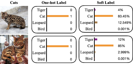
Figure 1: As seen from the coloration patterns of the two cats, the cat in the first row is more visually similar to a leopard while the cat in the second row is more visually similar to a tiger. Instead of assigning them the same one-hot label, it is reasonable to assign them different soft labels with different probabilities for different classes.

Coinciding with the above idea, many approaches have benefited from soft labels which assign small probabilities to non-ground-truth classes. The label smoothing regularizer (LSR) (Müller, Kornblith, and Hinton 2019; Szegedy et al. 2016) which uses soft labels generated by interpolating one-hot labels and uniform-distribution labels has improved the performances on image classification (Szegedy et al. 2016; Zoph et al. 2018; Real et al. 2019), speech recognition (Chorowski and Jaitly 2016), and machine translation (Vaswani et al. 2017), but LSR is unable to capture instance-to-class similarities, e.g., some cats are more visually similar to tigers while some other cats are more similar to leopards as illustrated in Figure 1. Knowledge distillation (KD) (Hinton, Vinyals, and Dean 2015) takes advantage of the instance-level soft labels generated by a pretrained teacher network to train a student network, thus improving the student performance significantly. However, the training cost of KD is several times of that of the standard training procedure due to two factors: (1) KD first needs to train a teacher network; (2) when KD trains the student network, in each iteration, each image needs to be processed twice, once by the teacher network and once by the student network.

Instead of using a manually designed uniform distribution or a pretrained DNN to generate soft labels, we turn to the learned instance-to-class similarities in the past epochs. In the standard training procedure, all the learned information in the earlier epochs except the weights is discarded and the training process progresses by using one-hot labels all the time. Different from the standard training procedure, we propose to learn with retrospection (LWR) to make use of the learned information in the past epochs. Specifically, LWR generates and then updates the soft labels for each image by taking advantage of the output logits in the past epochs. The soft labels are then used to guide the training in the subsequent epochs, thus mitigating the overconfidence or overfitting issue. LWR is able to improve accuracies, robustness, and calibration of DNNs without introducing any additional network parameters, without increasing inference cost, and even without needing to further tune training hyperparameters (i.e., the learning rate scheme, the mini-batch size, the total epochs in the standard training procedure are all kept), but only with a negligible overhead for updating soft labels.

Our main contributions are summarized as follows:

• Different from the current standard training procedure which discards all the learned information in the past epochs except the learned weights, we propose to learn with retrospection (LWR) to make use of the learned information in the past epochs. LWR uses the learned instance-to-class similarities as soft labels to supervise the training in the subsequent epochs, thus alleviating overconfidence or overfitting.

• Extensive experiments on several benchmark datasets demonstrate that LWR significantly improves accuracies, robustness, and calibration of various modern networks, and outperforms the state-of-the-art label smoothing based approaches.

Related Work

Label Smoothing

(Szegedy et al. 2016) propose the label smoothing regularizer (LSR) that utilizes the weighted average of one-hot labels and the uniform distribution as soft labels, and successfully uses it to improve the performance of the Inception architecture on image classification. Ever since then, many advanced image classification approaches (Zoph et al. 2018; Real et al. 2019; Huang et al. 2019) have incorporated LSR into training procedures. Besides image classification, label smoothing has also been used in speech recognition to reduce the word error rate on the WSJ dataset (Chorowski and Jaitly 2016). Moreover, in machine translation, (Vaswani et al. 2017) show that label smoothing is able to improve the BLEU score but with a reduction in perplexity. (Müller, Kornblith, and Hinton 2019) empirically show that LSR is also able to improve the calibration of DNNs. (Pereyra et al. 2017) propose to smooth the output distribution of a DNN by penalizing low entropy predictions, which obtains consistent performance improvements across various tasks. Recently, (Yuan et al. 2020) propose a new manually designed label smoothing regularizer named TF-Reg which is developed from LSR but outperforms LSR. These label smoothing techniques can be considered as assigning the same small probability to the non-ground-truth classes, thus mitigating the overconfidence issue of DNNs. However, these approaches cannot fully utilize the advantages of label smoothing as they do not take into account class similarities.

Knowledge Distillation

KD (Hinton, Vinyals, and Dean 2015) is able to overcome the disadvantages of the manually designed label smoothing regularizers by taking advantage of the soft labels generated by a pretrained teacher network to train a student. However, the training cost of KD is several times of those of using manually designed regularizers, since KD needs to first train a powerful teacher, and does inference twice (i.e., once for the teacher and once for the student) for each training sample in each iteration when training the student network. To reduce the cost of training a powerful teacher which is usually larger than the student, many self-distillation approaches including but not limited to (Xu and Liu 2019; Zhang et al. 2019; Yang et al. 2019b, a; Furlanello et al. 2018; Bagherinezhad et al. 2018; Yun et al. 2020) have been proposed. (Zhang et al. 2019) propose to generate soft labels by adding additional basic blocks or layers to the shallow layers, which improves the performance but has a large computation and memory overhead. Born-again networks (Furlanello et al. 2018) and label-refine networks (Bagherinezhad et al. 2018) are based on the same idea but from different perspectives. These two approaches train a network in many generations and use the network in the $(i-1)$th generation as the teacher to train the network in the $i$th generation. In other words, these approaches do not pretrain a large teacher, but instead pretrain the network itself as its own teacher, and this process can be repeated many times. They still have a large training overhead as they need to train a network many times. SD (Yang et al. 2019b) borrows the idea from (Huang et al. 2017) by relying on a cyclic learning rate schedule (Loshchilov and Hutter 2017) to train DNNs in many mini-generations. Consequently, SD cannot use the optimal training hyper-parameters (e.g., training epochs and learning rate schemes) already searched in the standard training procedure for modern network architectures such as ResNet (He et al. 2016a) and VGG (Simonyan and Zisserman 2014). Moreover, this cyclic learning rate scheme also causes that SD cannot update the supervision information frequently. We also find that SD is prone to severe underconfidence.

Note that in this paper, we aim to propose a framework to improve the DNN performance with comparable training and inference costs to the standard training procedure. Thus, we do not compare the proposed method with those approaches (e.g., born-again and label-refine networks) whose training or inference cost is several times of ours.

Framework

In this section, we introduce LWR which trains a DNN with the assistance of itself in the past. To illustrate the connection between LWR and the standard training procedure, we first review the standard process for training DNNs on classification. Then we make further derivations of the standard process to show how to train DNNs with retrospection.

Standard Training Procedure

Given a training data set $\mathcal{D}$ = $(X,Y)$ = $\{(x_{i},y_{i})\}_{i=1}^{N}$ where $x_{i}$ is an input sample; $y_{i}$ is the corresponding one-hot label; and $N$ is the total number of training samples in $\mathcal{D}$, a DNN $f$ with parameters $\Theta$ is trained on $\mathcal{D}$. In the standard training procedure, the cross-entropy loss between DNN outputs and one-labels is minimized by a gradient descent based optimizer such as SGD with momentum or Adam (Kingma and Ba 2015). The DNN is trained for many epochs to well fit the data, where each epoch means going through all the samples in the training set once. Suppose that the number of total training epochs and the mini-batch size are $M$ and $B$, respectively. The total number of iterations in each epoch is $\lceil\frac{N}{B}\rceil$. In each iteration, a mini-batch of training samples ($\mathbf{x}$, $\mathbf{y}$) are sampled from $\mathcal{D}$ and then are fed into DNN $f$:

$$\mathbf{z}=f(\Theta,\mathbf{x})$$ (1)

Note that $\mathbf{z}$ are the output logits before softmax. Then the cross-entropy loss between the output logits and the one-hot labels are computed:

$$\mathcal{L}_{CE}=H(\sigma(\mathbf{z}),\mathbf{y})$$ (2)

where $H$ is cross-entropy and $\sigma(.)$ denotes softmax. Then parameters $\Theta$ are updated once in this iteration based on the gradients of $\mathcal{L}_{CE}$ with respect to $\Theta$.

From the beginning to the end of the training process, more and more information is learned with the observation that the training and validation accuracies are higher and higher. It indicates that even in the early iterations, there is still some useful information that has been learned. However, we notice that all the information learned in the previous iterations except the values of $\Theta$ is discarded in the standard training process. In light of this, we propose to learn with retrospection to make use of the learned information in the previous iterations to assist the subsequent training. An interesting problem is how to effectively use the learned information to assist the training in the subsequent iterations.

Learning with Retrospection

We propose LWR which takes advantage of the training logits in the previous epochs to generate soft labels to guide the training in the subsequent epochs. Thus, besides the one-hot label, each training data sample also has a soft label generated during the training process.

Making Use of Training Logits Instead of Discarding

In each iteration of the standard training procedure, training logits $\mathbf{z}$ of a mini-batch of samples are only used to compute cross-entropy loss (2) and then are discarded. We argue that the training logits contain instance-to-class similarities which may be useful for subsequent training. We take advantage of the training logits by using the softmax function with a temperature to generate soft labels:

$$\mathbf{s}=\sigma(\mathbf{z}/\tau)=\frac{exp(\mathbf{z}/\tau)}{\sum_{j}exp(\mathbf{z}[j]/\tau)}$$ (3)

where $\tau$ is a temperature to soften the logits and $z[j]$ are the logits corresponding to the $j$th class. As every training sample is processed once in each epoch, we can obtain the soft labels for all the training samples in each epoch.

Figure 2: Framework of LWR

Training DNNs with LWR

As shown in Figure 2, we update the soft labels once every $k$ epochs. In the first $k$ epochs, there are no soft labels and we just minimize the regular cross-entropy loss (2). After that, the training is supervised by both one-hot labels and soft labels. We denote the soft labels generated in the $(i\times k)$th epoch by $\mathbf{s}_{ik}$. $\mathbf{s}_{ik}$ are used to guide the training from the $(i\times k+1)$th epoch to the $((i+1)\times k)$th epoch with the following training objective:

$$\mathcal{L}_{LWR}=\alpha H(\sigma(\mathbf{z}),\mathbf{y})+\beta\tau^{2}K(\sigma(\mathbf{z}/\tau),\mathbf{s}_{ik})$$ (4)

where $K(.)$ denotes KL-divergence; $\alpha$ and $\beta$ are two balancing weights. Note that the gradients do not flow through $\mathbf{s}_{ik}$, since they are just the records of the previous epochs. As the soft labels are more and more accurate as the training process progresses, $\beta$ should be larger and larger and $\alpha$ should be smaller and smaller from the beginning to the end of the training process. Based on this idea, in most cases, we simply set $\alpha$ and $\beta$ to $(1-0.9\times\frac{i\times k}{M})$ and $(0.9\times\frac{i\times k}{M})$, respectively, where $M$ is the total number of training epochs. Thus, when LWR is introduced, almost only two hyperparameters, i.e., temperature $\tau$ and updating interval $k$, need to be tuned as LWR can use the training hyperparameters (i.e., total number of training epochs $M$, the learning rate scheme, and mini-batch size $B$) of the standard training procedure. The training overhead of LWR is the cost of storing a soft label for each image, which is negligible as these soft labels do not need to be stored in the GPU memory.

The implementation-level description of LWR is summarized in Algorithm 1.

Algorithm 1 LWR

1:Training data $\mathcal{D}$, DNN $f$ with parameter $\Theta$

2:Optimal $\Theta$

3:for $i=1,2,...,M$ epochs do

4:     if $i\leq k$ then

5:         Update $\Theta$ based on (2) by gradient descent

6:         if $i==k$ then

7:              Generate soft labels by (3)

8:         end if

9:     else

10:         Update $\Theta$ based on (4) by gradient descent

11:         if $i\%k==0$ then

12:              Update soft labels by (3)

13:         end if

14:     end if

15:end for

Why LWR Works

In this part, we provide an analysis of why LWR works.

Benefiting from Label Smoothing

LSR smooths one-hot label $y$ by using a weighted average of the one-hot label and a uniform distribution, i.e., $y_{LSR}=(1-\epsilon)*y+\epsilon/C$ where $\epsilon$ is a small factor and usually set to 0.1, and $C$ is the total number of classes. As shown in the existing literature (Müller, Kornblith, and Hinton 2019), LSR mitigates over-confidence of DNNs and improves DNN generalization and calibration. We notice that LSR is a special case of LWR. The training loss of LSR can be decomposed into two parts:

$$H(\sigma(\mathbf{z}),y_{LSR})=(1-\epsilon)H(\sigma(\mathbf{z}),y)+\epsilon H(\sigma(\mathbf{z}),\frac{1}{C})$$ (5)

It is observed that (5) shares a similar form to (4), and $K(\sigma(\mathbf{z}/\tau),\mathbf{s}_{ik})$ in (4) is equivalent to $H(\sigma(\mathbf{z}/\tau)),\mathbf{s}_{ik})$ plus a constant (i.e., the entropy of soft labels $\mathbf{s}_{ik}$). When $\tau$ is set to 1 and the learned soft label $\mathbf{s}_{ik}$ follows a uniform distribution, LWR is equivalent to LSR. Thus, LWR is an adaptive version of LSR, suggesting that it should inherit the advantages of LSR, such as better generalization and calibration.

Table 1: Test Accuracies (%) on CIFAR-100 and Tiny ImageNet. $\uparrow$ denotes the absolute improvement over the standard training procedure (i.e., STD).

		ResNet-56	WRN-16-4	ShuffleV2	VGG-16	PreAct ResNet-18
CIFAR -100	STD	72.00$\pm$0.16	76.43$\pm$0.16	71.12$\pm$0.39	74.16$\pm$0.28	77.31$\pm$0.33
	LSR	72.05$\pm$0.16	76.45$\pm$0.10	71.90$\pm$0.13	74.75$\pm$0.12	78.24$\pm$0.16
	Max-Entropy	72.03$\pm$0.19	76.47$\pm$0.15	71.23$\pm$0.22	74.11$\pm$0.13	77.65$\pm$0.35
	SD	72.22$\pm$0.20	77.00$\pm$0.38	68.70$\pm$0.51	74.28$\pm$0.35	78.31$\pm$0.24
	CS-KD	72.05$\pm$0.19	76.28$\pm$0.11	71.43$\pm$0.28	74.61$\pm$0.12	78.01$\pm$0.13
	TF-Reg	72.11$\pm$0.29	76.52$\pm$0.28	72.09$\pm$0.34	74.69$\pm$0.18	77.36$\pm$0.23
	LWR (Ours)	74.25$\pm$0.29 ($\uparrow$ 2.25)	77.88$\pm$0.27 ($\uparrow$ 1.45)	73.53$\pm$0.33 ($\uparrow$ 2.41)	75.24$\pm$0.09 ($\uparrow$ 1.08)	79.73$\pm$0.32 ($\uparrow$ 2.42)
Tiny ImageNet	STD	56.31$\pm$0.05	59.48$\pm$0.16	60.80$\pm$0.25	62.39$\pm$0.45	65.57$\pm$0.16
	LSR	56.57$\pm$0.38	59.33$\pm$0.16	61.85$\pm$0.27	63.82$\pm$0.03	64.91$\pm$0.08
	Max-Entropy	56.80$\pm$0.41	59.06$\pm$0.19	61.56$\pm$0.40	62.99$\pm$0.12	65.25$\pm$0.16
	SD	57.52$\pm$0.17.	59.68$\pm$0.13	60.79$\pm$0.15	63.14$\pm$0.16	65.87$\pm$0.28
	CS-KD	56.21$\pm$0.41	59.92$\pm$0.29	61.66$\pm$0.34	62.87$\pm$0.20	64.29$\pm$0.25
	TF-Reg	56.43$\pm$0.19	59.41$\pm$0.10	61.55$\pm$0.42	62.95$\pm$0.06	64.88$\pm$0.47
	LWR (Ours)	57.95$\pm$0.25 ($\uparrow$ 1.64)	61.22$\pm$0.29 ($\uparrow$ 1.74)	62.06$\pm$0.29 ($\uparrow$1.26)	64.42$\pm$0.06 ($\uparrow$ 2.03 )	66.40$\pm$0.12 ($\uparrow$ 0.83)

Table 2: Test Accuracies (%) on fine-grained classification datasets. $\uparrow$ denotes the absolute improvement over the STD procedure.

		ResNet-10	ResNet-18	MobileNetV2	ShuffleNetV2
CUB	STD	58.96$\pm$0.12	61.09$\pm$0.49	67.20$\pm$0.21	61.67$\pm$0.85
	LSR	59.31$\pm$0.21	63.57$\pm$0.50	67.97$\pm$0.43	62.66$\pm$0.11
	Max-Entropy	59.00$\pm$0.30	61.23$\pm$0.37	66.56$\pm$0.30	61.10$\pm$0.15
	SD	59.28$\pm$0.34	64.19$\pm$0.24	68.15$\pm$0.32	63.99$\pm$0.29
	CS-KD	60.70$\pm$0.21	64.57$\pm$0.29	67.48$\pm$0.32	63.32$\pm$0.25
	TF-Reg	58.84$\pm$0.60	62.04$\pm$0.28	67.20$\pm$0.43	61.19$\pm$0.58
	LWR (Ours)	63.14$\pm$0.17 ($\uparrow$ 4.18)	66.47$\pm$0.37 ($\uparrow$ 5.38)	69.00$\pm$0.41 ($\uparrow$ 1.80)	64.37$\pm$0.52 ($\uparrow$ 2.70)
Stanford Dogs	STD	63.91$\pm$0.25	66.56$\pm$0.28	68.05$\pm$0.26	66.08$\pm$0.32
	LSR	63.36$\pm$0.03	67.12$\pm$0.86	69.13$\pm$0.09	66.90$\pm$0.34
	Max-Entropy	63.94$\pm$0.30	66.42$\pm$0.50	67.97$\pm$0.30	66.25$\pm$0.60
	SD	64.65$\pm$0.36	68.79$\pm$0.06	70.26$\pm$0.35	67.30$\pm$0.26
	CS-KD	64.91$\pm$0.26	69.17$\pm$0.19	68.73$\pm$0.25	66.75$\pm$0.31
	TF-Reg	63.72$\pm$0.44	66.53$\pm$0.50	68.36$\pm$0.26	66.63$\pm$0.26
	LWR (Ours)	66.28$\pm$0.15 ($\uparrow$ 2.37)	69.84$\pm$0.45 ($\uparrow$ 3.28)	70.45$\pm$0.12 ($\uparrow$ 2.40)	67.39$\pm$0.42 ($\uparrow$ 1.31)
FGVC-Aircraft	STD	73.89$\pm$0.25	79.58$\pm$0.25	83.01$\pm$0.30	78.00$\pm$0.45
	LSR	74.52$\pm$0.18	80.91$\pm$0.28	83.88$\pm$0.10	78.40$\pm$0.94
	Max-Entropy	73.39$\pm$0.09	79.59$\pm$0.41	82.81$\pm$0.45	78.20$\pm$0.25
	SD	74.98$\pm$0.38	80.55$\pm$0.80	83.36$\pm$0.13	78.09$\pm$0.34
	CS-KD	74.95$\pm$0.40	79.72$\pm$0.19	80.62$\pm$0.38	77.89$\pm$1.55
	TF-Reg	73.69$\pm$0.38	80.12$\pm$0.33	83.39$\pm$0.11	78.50$\pm$0.31
	LWR (Ours)	76.41$\pm$0.26 ($\uparrow$ 2.52)	81.25$\pm$0.05 ($\uparrow$ 1.67)	84.56$\pm$0.54 ($\uparrow$ 1.55)	78.59$\pm$0.37 ($\uparrow$ 0.59)

Table 3: Test Accuracies (%) on Tabular Datasets

	Abalone	Arcene	Iris
STD	25.75$\pm$0.26	83.00$\pm$2.16	90.00$\pm$2.72
LSR	26.75$\pm$0.54	81.00$\pm$4.55	92.22$\pm$1.57
Max-H	27.15$\pm$1.17	79.67$\pm$3.77	94.44$\pm$1.57
SD	25.79$\pm$0.91	81.00$\pm$1.63	93.33$\pm$2.72
CS-KD	27.70$\pm$1.08	83.67$\pm$0.94	94.44$\pm$1.57
TF-Reg	25.87$\pm$0.52	80.00$\pm$2.16	90.00$\pm$2.72
LWR (Ours)	31.86$\pm$0.51	85.33$\pm$1.25	95.56$\pm$1.57

Benefiting from Instance-level Class Similarities

One-hot labels set the probability for the ground-truth class to 1 while the probabilities for the other classes are all set to 0. This may cause overfitting or overconfidence issues especially when the training samples in different classes share visual or semantic similarities. Maximizing the ground-truth probability while preserving small probabilities for the other classes may mitigate this issue. It is principled to use class similarities as the soft labels which assign corresponding probabilities to different classes. Note that class similarities may not well represent instance-to-class similarities because different training samples in the same class may be close to different classification boundaries. For example, some cats are more visually similar to dogs while some other cats are more similar to tigers. This kind of instance-level class similarities is learned gradually during the training process. Motivated by this observation, LWR takes advantage of the training logits to generate instance-level soft labels. Therefore, LWR also benefits from the learned instance-to-class similarities during the training process.

Experiments

Experimental Setup

Datasets

We report the results on several benchmark datasets, i.e., CIFAR-10 (Krizhevsky and Hinton 2009), CIFAR-100 (Krizhevsky and Hinton 2009), Tiny ImageNet , CUB-200-2011 (Wah et al. 2011), Stanford Dogs (Khosla et al. 2011), FGVC-Aircraft (Maji et al. 2013), Abalone (Dua and Graff 2017), Arcene (Dua and Graff 2017), and Iris (Dua and Graff 2017). CIFAR-10 is a 10-class image classification dataset, containing 50,000 training images and 10,000 test images. CIFAR-100 has similar images to those in CIFAR-10, but has 100 classes. Tiny ImageNet, i.e., a subset of ImageNet, has 200 classes, containing 100,000 training images and 10,000 test images. CUB-200-2011, Stanford Dogs, and FGVC-Aircraft are three fine-grained classification datasets, containing 11,788 images of 200 bird species, 22,000 images of 120 breeds of dogs, and 10,200 images of 102 different aircraft model variants, respectively. Abalone, Arcene, and Iris are three tabular datasets which are randomly drawn from UCI datasets (Dua and Graff 2017). We follow the default training and test splits. We use the standard data augmentation strategy for image datasets, i.e., randomly flipping horizontally, padding, and then randomly cropping. More details are presented in the Appendix.

Architectures

To check whether LWR is able to work on different network architectures, we adopt a variety of modern architectures including ResNet (He et al. 2016a), PreAct ResNet (He et al. 2016b), VGG (Simonyan and Zisserman 2014), WRN (Zagoruyko and Komodakis 2016), MobileNet (Sandler et al. 2018), and ShuffleNet (Ma et al. 2018).

Competitors

We compare LWR with the standard training procedure and label smoothing based methods including cost-comparable self-distillation methods: (1) STD: STD trains a DNN by minimizing the regular cross-entropy loss between output logits and one-hot labels; (2) LSR (Müller, Kornblith, and Hinton 2019; Szegedy et al. 2016): LSR uses the weighted average of one-hot labels and a uniform distribution as targets to train a DNN. (3) Max-Entropy (Pereyra et al. 2017): Max-Entropy smooths the DNN output by maximizing its entropy. (4) SD (Yang et al. 2019b): SD is a self-distillation method that relies on a periodic learning rate scheme to train a DNN. (5) CS-KD (Yun et al. 2020): CS-KD distills the predictive distribution of different samples from the same class. (6) TF-Reg (Yuan et al. 2020): TF-Reg modifies LSR to generate more accurate soft labels.

Hyperparameters

Following the standard training procedure for modern DNNs, we have trained all the networks for 200 epochs with optimizer SGD with momentum 0.9 and weight decay 5e-4 on CIFAR, CUB-200-2011, Stanford Dogs, and FGVC-Aircraft, 120 epochs for Tiny ImageNet. More implementation details are reported in Appendix. For all the competitors, we report the author-reported results or use author-provided codes and the optimal hyper-parameters from the original papers if they are publicly available. Otherwise, we use our implementation. We report the test accuracy in the last epoch unless otherwise specified. All the results below are reported based on 3 runs.

Table 4: ECE (%) Results. For ECE, the lower is better. $\downarrow$ denotes the absolute ECE reduction below the STD training procedure.

	CIFAR-100		Tiny ImageNet
	ShuffleNetV2	Preact ResNet-18	ShuffleNetV2	Preact ResNet-18
STD	12.60$\pm$0.16	7.52$\pm$0.30	10.12$\pm$0.22	11.04$\pm$0.11
LSR	3.16$\pm$0.47	10.81$\pm$0.44	2.89$\pm$0.15	8.33$\pm$0.43
Max-Entropy	13.87$\pm$0.24	8.41$\pm$0.14	11.88$\pm$0.47	13.43$\pm$0.11
SD	28.63$\pm$0.38	32.74$\pm$0.18	25.34$\pm$0.50	31.03$\pm$0.21
CS-KD	8.84$\pm$0.19	4.69$\pm$0.56	5.33$\pm$0.31	6.66$\pm$0.43
TF-Reg	3.25$\pm$0.20	10.76$\pm$0.14	8.16$\pm$0.43	9.13$\pm$0.42
LWR (Ours)	2.87$\pm$0.06 ($\downarrow$ 9.73)	3.53$\pm$0.13 ($\downarrow$ 3.99)	4.30$\pm$0.33 ($\downarrow$ 5.82)	1.58$\pm$0.32 ($\downarrow$ 9.46)

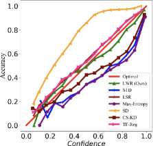
Figure 3: ShuffleNetV2 on CIFAR-100

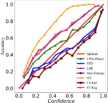
Figure 4: Preact ResNet-18 on CIFAR-100

Figure 5: ShuffleNetV2 on Tiny ImageNet

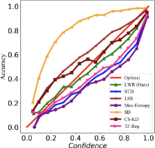
Figure 6: Preact ResNet-18 on Tiny ImageNet

Classification Accuracy

Regular Classification

We use CIFAR-100 and Tiny ImageNet datasets for regular classification. The results are reported in Table 1. It is observed that by simply learning from the past, LWR improves the performances by a large margin over the standard training procedure (i.e., STD) on both datasets across various modern DNN architectures, and also outperforms all the other label smoothing based approaches significantly, which demonstrates the effectiveness of LWR.

Fine-grained Classification

We adpot CUB-200-2011, Stanford Dogs, and FGVC-Aircraft datasets for fine-grained classification. Table 2 reports the comparison results on these three fine-grained datasets. LWR obtains much better performances than those of the standard training procedure and the other label smoothing based approaches. Overall, the superiority of LWR becomes more obvious on fine-grained datasets. This is not surprising due to the following facts: (1) fine-grained image classification contains more visually similar classes; (2) STD uses one-hot labels which are orthogonal for different classes, ignoring class similarities; (3) in contrast, LWR takes advantage of soft labels which contain instance-to-class similarities. This also implies that the instance-to-class similarity is significantly important for fine-grained classification.

Tabular Data Classification

To evaluate LWR on non-image data, we conduct a series of experiments on three tabular datasets which are randomly drawn from the UCI dataset. We follow (Zhang et al. 2018) and adopt the neural network with two hidden, fully-connected layers of 128 units. We train it for 50 epochs with mini-batche size 16 by using Adam (Kingma and Ba 2015) with default hyper-parameters. As shown in Table 3, LWR improves 6.11%, 2.33%, and 5.56% of the accuracies over the strand training procedure on the three datasets, respectively, and outperforms the other approaches significantly, which demonstrates the applicability of LWR on non-image data.

Table 5: Robustness Results with Preact ResNet-18 on CIFAR-10 with different levels of noise

Noise	Accuracy	STD	LSR	SD	CS-KD	TF-Reg	LWR(Ours)
20%	Last	83.81$\pm$0.13	84.21$\pm$0.41	90.13$\pm$0.17	83.62$\pm$0.15	83.89$\pm$0.69	93.80$\pm$0.13 ($\uparrow$ 9.99)
	Best	91.78$\pm$0.07	91.77$\pm$0.18	90.72$\pm$0.21	85.69$\pm$0.23	91.85$\pm$0.15	94.17$\pm$0.04 ($\uparrow$ 2.39)
40%	Last	66.32$\pm$0.56	66.93$\pm$0.92	83.22$\pm$0.74	69.51$\pm$0.51	65.77$\pm$2.39	89.14$\pm$0.30 ($\uparrow$ 22.82)
	Best	88.89$\pm$0.06	89.41$\pm$0.25	86.57$\pm$0.20	84.00$\pm$0.68	88.96$\pm$0.12	89.43$\pm$0.32 ($\uparrow$ 0.54)
60%	Last	45.05$\pm$0.71	46.35$\pm$1.24	75.01$\pm$0.27	49.90$\pm$0.45	45.01$\pm$1.05	86.19$\pm$0.05 ($\uparrow$ 41.14)
	Best	84.38$\pm$0.14	84.74$\pm$0.06	81.17$\pm$0.17	77.39$\pm$0.98	84.51$\pm$0.06	87.27$\pm$0.08 ($\uparrow$ 2.89)
80%	Last	27.08$\pm$1.51	26.18$\pm$0.49	65.79$\pm$0.68	27.82$\pm$0.51	26.52$\pm$0.26	72.27$\pm$0.19 ($\uparrow$ 45.19)
	Best	73.32$\pm$0.23	73.04$\pm$0.23	71.14$\pm$0.33	60.07$\pm$1.42	72.12$\pm$0.38	78.72$\pm$0.10 ($\uparrow$ 5.40)

Table 6: Effects of updating interval $k$ and temperature $\tau$ in terms of test accuracy (%) on CIFAR-100

		k=1	k=5	k=10	k=20	k=50	k=100
$\tau$=5	PreAct ResNet-18	79.50$\pm$0.10	79.73$\pm$0.22	79.27$\pm$0.10	78.67$\pm$0.52	78.46$\pm$0.51	76.32$\pm$0.11
	ResNet-56	73.40$\pm$0.31	74.25$\pm$0.29	73.87$\pm$0.15	73.37$\pm$0.17	73.53$\pm$0.27	72.98$\pm$0.23
	WRN-16-4	77.88$\pm$0.27	77.64$\pm$0.39	77.63$\pm$0.18	77.60$\pm$0.22	77.37$\pm$0.29	76.60$\pm$0.09
	ShuffleNetV2	73.45$\pm$0.05	73.53$\pm$0.33	73.55$\pm$0.30	73.33$\pm$0.11	73.20$\pm$0.19	72.50$\pm$0.03
	VGG-16	74.97$\pm$0.08	75.05$\pm$0.07	74.94$\pm$0.16	75.24$\pm$0.11	75.24$\pm$0.09	74.13$\pm$0.27
$\tau$=10	PreAct ResNet-18	79.39$\pm$0.30	79.12$\pm$0.03	79.60$\pm$0.17	78.95$\pm$0.11	78.24$\pm$0.27	76.50$\pm$0.38
	ResNet-56	73.66$\pm$0.15	73.40$\pm$0.30	73.62$\pm$0.29	73.65$\pm$0.17	73.81$\pm$0.19	72.62$\pm$0.40
	WRN-16-4	77.17$\pm$0.14	77.43$\pm$0.20	77.23$\pm$0.12	77.84$\pm$0.13	77.38$\pm$0.33	76.64$\pm$0.12
	ShuffleNetV2	73.29$\pm$0.20	72.89$\pm$0.37	73.55$\pm$0.24	73.16$\pm$0.10	73.57$\pm$0.34	72.89$\pm$0.09
	VGG-16	74.78$\pm$0.36	74.87$\pm$0.32	74.88$\pm$0.14	75.14$\pm$0.26	75.27$\pm$0.28	74.15$\pm$0.16

Calibration

With the deployment of DNNs in high-risk domains, predictive uncertainty of DNNs is of increasing importance. The predictive confidence of a well-calibrated classifier should be indicative of the accuracy. Following the existing work (Guo et al. 2017; Müller, Kornblith, and Hinton 2019), we use Expected Calibration Error (ECE) and Reliability Diagrams to measure the calibration effects. Specifically, ECE is the expected difference between confidence scores (i.e., the winning softmax scores) and accuracies. It is calculated by partitioning classifier predictions into $M$ bins of equal size and taking a weighted average of differences between confidence scores and accuracies in the bins:

$$ECE=\sum_{m=1}^{M}\frac{\left|B_{m}\right|}{n}\left|acc\left(B_{m}\right)-conf\left(B_{m}\right)\right|$$ (6)

where $n$ is the total number of samples; $B_{m}$ is the set of samples whose confidence scores fall into bin $m$; $\left|B_{m}\right|$ denotes the number of samples in $B_{m}$; $acc(B_{m})$ is the accuracy of $B_{m}$; and $conf(B_{m})$ is the average confidence of $B_{m}$.

Table 4 reports the ECE of different approaches. LWR improves the calibration over the standard training procedure consistently and significantly. As expected, in most cases, LWR and LSR perform better than the other approaches, and overall LWR outperforms all the other competitors.

To better understand the overconfidence or underconfidence issue of different approaches, we plot the reliability diagrams of these approaches. The reliability diagram plots the expected accuracy as a function of the confidence. Thus, the identity function implies the optimal calibration. Figure 6, Figure 6, Figure 6, and Figure 6 show the reliability diagrams of different approaches on CIFAT-100 and Tiny ImageNet with ShuffleNetV2 and Preact ResNet-18. We plot the red line (i.e., the identity function) to represent the optimal calibration. We have the following observations: (1) LWR, LSR, and TF-Reg are closer to the optimal calibration than the other approaches, which demonstrates the effectiveness of LWR on calibration; (2) STD and Max-Entropy are prone to overconfidence, where the overconfidence of STD has also been observed by the existing studies (Guo et al. 2017; Müller, Kornblith, and Hinton 2019); (3) SD suffers from severe underconfidence; (4) The calibration of CS-KD varies with datasets. Specifically, it is overconfident on CIFAR-100 but well calibrated on Tiny ImageNet.

Robustness

As DNNs have been applied to security-critical tasks such as autonomous driving and medical diagnosis, the robustness of DNNs becomes extraordinarily important. Following the existing study (Zhang et al. 2017), we use CIFRA-10 with different levels of corrupted labels to evaluate the robustness of different approaches. Specifically, we use the open-source implementation of (Zhang et al. 2017) to generate four CIFAR-10 training sets, where 20%, 40%, 60%, and 80% of the labels are replaced with random noise, respectively. All the test labels are kept intact for evaluation.

The results are summarized in Table 5, where we report the test accuracy in the last epoch (i.e., the 200th epoch) and the best test accuracy achieved during the training process. First, we notice that there is a large gap between the last accuracy and the best accuracy for most approaches. The reason is that as the training progresses, the DNN overfits the noise in the later epochs. (Arpit et al. 2017; Han et al. 2018) have a similar observation that DNNs first memorize training data with clean labels and then those with noisy labels. Especially, when the noise rate is 80%, the DNN trained with STD overfits a large amount of noise at later epochs, which leads to an extremely large accuracy gap between the last epoch and the best epoch. However, LWR significantly mitigates this issue as LWR makes use of the information in the past epochs instead of overfitting noise. As expected, LWR improves the robustness of DNNs significantly.

Effects of Interval $k$ and Temperature $\tau$

Interval $k$ denotes updating soft labels once every $k$ epochs, and temperature $\tau$ controls the softness of the labels. We check their effects on the performance of LWR. Table 6 summarizes their effects across different DNN architectures on CIFAR-100. It is not surprising that when interval $k$ is smaller than a threshold (i.e., the updating frequency is greater than a number), LWR works reasonably well, and when $k$ is set to a large number (e.g., 100), the performances drop significantly. On the other hand, the best performances of almost all the networks are obtained when $\tau$ is set to 5 rather than 10. The reason can be that as seen from (3), setting $\tau$ to a large number leads to a flat distribution, which may weaken the information in the soft labels.

Conclusion and Future Work

It is observed that samples in different classes usually share some visual or semantic similarities. However, the typically used one-hot labels cannot capture this kind of information as they are orthogonal for different classes. On the other hand, we also observe that the standard training procedure discards all the information learned in the past epochs except the weights. Motivated by these observations, we propose LWR to make use of the learned information in the past to guide the subsequent training. Specifically, the training logits in the past epochs are used to generate soft labels to provide supervision for the subsequent training. LWR benefits from label smoothing effects and instance-to-class similarities. To the end, LWR is able to improve accuracies, calibration, and robustness of DNNs without introducing any network parameters, without any additional inference cost, but only with a negligible training overhead. Extensive experiments on several datasets have demonstrated the effectiveness of LWR across various modern network architectures.

We have applied this idea of learning from the past on classification by proposing LWR. Besides classification, the idea is expected to generalize to regression. We leave the question on how to use the past learned information in training regression tasks to the future work.

References

- Arpit et al. (2017) Arpit, D.; Jastrzebski, S. K.; Ballas, N.; Krueger, D.; Bengio, E.; Kanwal, M. S.; Maharaj, T.; Fischer, A.; Courville, A. C.; Bengio, Y.; et al. 2017. A Closer Look at Memorization in Deep Networks. In ICML.
- Bagherinezhad et al. (2018) Bagherinezhad, H.; Horton, M.; Rastegari, M.; and Farhadi, A. 2018. Label refinery: Improving imagenet classification through label progression. arXiv preprint arXiv:1805.02641 .
- Chorowski and Jaitly (2016) Chorowski, J.; and Jaitly, N. 2016. Towards better decoding and language model integration in sequence to sequence models. arXiv preprint arXiv:1612.02695 .
- Dua and Graff (2017) Dua, D.; and Graff, C. 2017. UCI Machine Learning Repository. URL http://archive.ics.uci.edu/ml.
- Furlanello et al. (2018) Furlanello, T.; Lipton, Z. C.; Tschannen, M.; Itti, L.; and Anandkumar, A. 2018. Born again neural networks. arXiv preprint arXiv:1805.04770 .
- Guo et al. (2017) Guo, C.; Pleiss, G.; Sun, Y.; and Weinberger, K. Q. 2017. On calibration of modern neural networks. arXiv preprint arXiv:1706.04599 .
- Han et al. (2018) Han, B.; Yao, Q.; Yu, X.; Niu, G.; Xu, M.; Hu, W.; Tsang, I.; and Sugiyama, M. 2018. Co-teaching: Robust training of deep neural networks with extremely noisy labels. In Advances in neural information processing systems, 8527–8537.
- He et al. (2016a) He, K.; Zhang, X.; Ren, S.; and Sun, J. 2016a. Deep residual learning for image recognition. In Proceedings of the IEEE conference on computer vision and pattern recognition, 770–778.
- He et al. (2016b) He, K.; Zhang, X.; Ren, S.; and Sun, J. 2016b. Identity mappings in deep residual networks. In European conference on computer vision, 630–645. Springer.
- Hinton, Vinyals, and Dean (2015) Hinton, G.; Vinyals, O.; and Dean, J. 2015. Distilling the knowledge in a neural network. arXiv preprint arXiv:1503.02531 .
- Huang et al. (2017) Huang, G.; Li, Y.; Pleiss, G.; Liu, Z.; Hopcroft, J. E.; and Weinberger, K. Q. 2017. Snapshot ensembles: Train 1, get m for free. arXiv preprint arXiv:1704.00109 .
- Huang et al. (2019) Huang, Y.; Cheng, Y.; Bapna, A.; Firat, O.; Chen, D.; Chen, M.; Lee, H.; Ngiam, J.; Le, Q. V.; Wu, Y.; et al. 2019. Gpipe: Efficient training of giant neural networks using pipeline parallelism. In Advances in neural information processing systems, 103–112.
- Khosla et al. (2011) Khosla, A.; Jayadevaprakash, N.; Yao, B.; and Li, F.-F. 2011. Novel dataset for fine-grained image categorization: Stanford dogs. In Proc. CVPR Workshop on Fine-Grained Visual Categorization (FGVC), volume 2.
- Kingma and Ba (2015) Kingma, D. P.; and Ba, J. 2015. Adam: A method for stochastic optimization. International Conference for Learning Representations .
- Krizhevsky and Hinton (2009) Krizhevsky, A.; and Hinton, G. 2009. Learning multiple layers of features from tiny images. Technical report, Citeseer.
- Lawrence et al. (1997) Lawrence, S.; Giles, C. L.; Tsoi, A. C.; and Back, A. D. 1997. Face recognition: A convolutional neural-network approach. IEEE transactions on neural networks 8(1): 98–113.
- Levinson et al. (2011) Levinson, J.; Askeland, J.; Becker, J.; Dolson, J.; Held, D.; Kammel, S.; Kolter, J. Z.; Langer, D.; Pink, O.; Pratt, V.; et al. 2011. Towards fully autonomous driving: Systems and algorithms. In 2011 IEEE Intelligent Vehicles Symposium (IV), 163–168. IEEE.
- Loshchilov and Hutter (2017) Loshchilov, I.; and Hutter, F. 2017. Sgdr: Stochastic gradient descent with warm restarts. International Conference for Learning Representations .
- Ma et al. (2018) Ma, N.; Zhang, X.; Zheng, H.-T.; and Sun, J. 2018. Shufflenet v2: Practical guidelines for efficient cnn architecture design. In Proceedings of the European conference on computer vision (ECCV), 116–131.
- Maji et al. (2013) Maji, S.; Kannala, J.; Rahtu, E.; Blaschko, M.; and Vedaldi, A. 2013. Fine-Grained Visual Classification of Aircraft. Technical report.
- Miotto et al. (2016) Miotto, R.; Li, L.; Kidd, B. A.; and Dudley, J. T. 2016. Deep patient: an unsupervised representation to predict the future of patients from the electronic health records. Scientific reports 6(1): 1–10.
- Müller, Kornblith, and Hinton (2019) Müller, R.; Kornblith, S.; and Hinton, G. E. 2019. When does label smoothing help? In Advances in Neural Information Processing Systems, 4694–4703.
- Pereyra et al. (2017) Pereyra, G.; Tucker, G.; Chorowski, J.; Kaiser, Ł.; and Hinton, G. 2017. Regularizing neural networks by penalizing confident output distributions. arXiv preprint arXiv:1701.06548 .
- Real et al. (2019) Real, E.; Aggarwal, A.; Huang, Y.; and Le, Q. V. 2019. Regularized evolution for image classifier architecture search. In Proceedings of the aaai conference on artificial intelligence, volume 33, 4780–4789.
- Sandler et al. (2018) Sandler, M.; Howard, A.; Zhu, M.; Zhmoginov, A.; and Chen, L.-C. 2018. Mobilenetv2: Inverted residuals and linear bottlenecks. In Proceedings of the IEEE conference on computer vision and pattern recognition, 4510–4520.
- Simonyan and Zisserman (2014) Simonyan, K.; and Zisserman, A. 2014. Very deep convolutional networks for large-scale image recognition. arXiv preprint arXiv:1409.1556 .
- Szegedy et al. (2016) Szegedy, C.; Vanhoucke, V.; Ioffe, S.; Shlens, J.; and Wojna, Z. 2016. Rethinking the inception architecture for computer vision. In Proceedings of the IEEE conference on computer vision and pattern recognition, 2818–2826.
- Vaswani et al. (2017) Vaswani, A.; Shazeer, N.; Parmar, N.; Uszkoreit, J.; Jones, L.; Gomez, A. N.; Kaiser, Ł.; and Polosukhin, I. 2017. Attention is all you need. In Advances in neural information processing systems, 5998–6008.
- Wah et al. (2011) Wah, C.; Branson, S.; Welinder, P.; Perona, P.; and Belongie, S. 2011. The caltech-ucsd birds-200-2011 dataset .
- Xu and Liu (2019) Xu, T.-B.; and Liu, C.-L. 2019. Data-distortion guided self-distillation for deep neural networks. In Proceedings of the AAAI Conference on Artificial Intelligence, volume 33, 5565–5572.
- Yang et al. (2019a) Yang, C.; Xie, L.; Qiao, S.; and Yuille, A. L. 2019a. Training deep neural networks in generations: A more tolerant teacher educates better students. In Proceedings of the AAAI Conference on Artificial Intelligence, volume 33, 5628–5635.
- Yang et al. (2019b) Yang, C.; Xie, L.; Su, C.; and Yuille, A. L. 2019b. Snapshot distillation: Teacher-student optimization in one generation. In Proceedings of the IEEE Conference on Computer Vision and Pattern Recognition, 2859–2868.
- Yuan et al. (2020) Yuan, L.; Tay, F. E.; Li, G.; Wang, T.; and Feng, J. 2020. Revisiting Knowledge Distillation via Label Smoothing Regularization. In Proceedings of the IEEE/CVF Conference on Computer Vision and Pattern Recognition, 3903–3911.
- Yun et al. (2020) Yun, S.; Park, J.; Lee, K.; and Shin, J. 2020. Regularizing class-wise predictions via self-knowledge distillation. In Proceedings of the IEEE/CVF Conference on Computer Vision and Pattern Recognition, 13876–13885.
- Zagoruyko and Komodakis (2016) Zagoruyko, S.; and Komodakis, N. 2016. Wide Residual Networks. In BMVC.
- Zhang et al. (2017) Zhang, C.; Bengio, S.; Hardt, M.; Recht, B.; and Vinyals, O. 2017. Understanding deep learning requires rethinking generalization. International Conference for Learning Representations .
- Zhang et al. (2018) Zhang, H.; Cisse, M.; Dauphin, Y. N.; and Lopez-Paz, D. 2018. mixup: Beyond empirical risk minimization. International Conference for Learning Representations .
- Zhang et al. (2019) Zhang, L.; Song, J.; Gao, A.; Chen, J.; Bao, C.; and Ma, K. 2019. Be your own teacher: Improve the performance of convolutional neural networks via self distillation. In Proceedings of the IEEE International Conference on Computer Vision, 3713–3722.
- Zoph et al. (2018) Zoph, B.; Vasudevan, V.; Shlens, J.; and Le, Q. V. 2018. Learning transferable architectures for scalable image recognition. In Proceedings of the IEEE conference on computer vision and pattern recognition, 8697–8710.