\savesymbol

AND

Stochastic Steepest Descent Methods for Linear Systems: Greedy Sampling & Momentum

\nameMd Sarowar Morshed \emailmorshed.m@northeastern.edu
\addrDepartment of Mechanical & Industrial Engineering
Northeastern University
Boston, MA, USA
\AND\nameSabbir Ahmad \emailahmad.sab@northeastern.edu
\addrKhoury College of Computer Sciences
Northeastern University
Boston, MA, USA
\AND\nameMd Noor-E-Alam \emailmnalam@neu.edu
\addrDepartment of Mechanical & Industrial Engineering
Northeastern University
Boston, MA, USA
Abstract

Recently proposed adaptive Sketch & Project (SP) methods connect several well-known projection methods such as Randomized Kaczmarz (RK), Randomized Block Kaczmarz (RBK), Motzkin Relaxation (MR), Randomized Coordinate Descent (RCD), Capped Coordinate Descent (CCD) etc. into one framework for solving linear systems. In this work, we first propose a Stochastic Steepest Descent (SSD) framework that connects SP methods with the well-known Steepest Descent (SD) method for solving positive-definite linear system of equations. We then introduce two greedy sampling strategies in the SSD framework that allow us to obtain algorithms such as Sampling Kaczmarz Motzkin (SKM), Sampling Block Kaczmarz (SBK), Sampling Coordinate Descent (SCD), etc. In doing so, we generalize the existing sampling rules into one framework and develop an efficient version of SP methods. Furthermore, we incorporated the Polyak momentum technique into the SSD method to accelerate the resulting algorithms. We provide global convergence results for both the SSD method and the momentum induced SSD method. Moreover, we prove $\mathcal{O}(\frac{1}{k})$ convergence rate for the Cesaro average of iterates generated by both methods. By varying parameters in the SSD method, we obtain classical convergence results of the SD method as well as the SP methods as special cases. We design computational experiments to demonstrate the performance of the proposed greedy sampling methods as well as the momentum methods. The proposed greedy methods significantly outperform the existing methods for a wide variety of datasets such as random test instances as well as real-world datasets (LIBSVM, sparse datasets from matrix market collection). Finally, the momentum algorithms designed in this work accelerate the algorithmic performance of the SSD methods.

Keywords: Steppest Descent Method, Kaczmarz Method, Coordinate Descent Method, Sketch & Project Method, Randomized Algorithms, Linear System, Heavy Ball Momentum.

1 Introduction

In this paper, we focus on solving the following fundamental problem:

$\displaystyle x^{*}=\operatorname*{arg\,min}_{x\in\mathbb{R}^{n}}\|x-t\|^{2}_{G}\quad\textbf{subject to}\quad Ax=b.$ (1)

where $G\in\mathbb{R}^{n\times n}$ is a symmetric positive definite matrix and $t\in\mathbb{R}^{n}$ is an arbitrary vector. Problem (1) is prevalent and central in a wide range of quantitative areas such as Numerical Linear Algebra, Computer Science, Scientific Computing, Machine Learning, Computer Vision, Optimization, Signal Processing, Financial Engineering, etc. From a Machine Learning perspective, problem (1) arises from a wide range of applications such as Gaussian processes (Rasmussen and Williams, 2008), Least-Square Support Vector Machines (Ye and Xiong, 2007), graph-based Semi-Supervised Learning and Graph-Laplacian problems (Bengio et al., 2006), Gaussian Markov Random Fields (Rue and Held, 2005), etc. Approximate solutions of Linear Systems can be of practical benefit in inexact Newton schemes (Jiang et al., 2012; Wang and Xu, 2013; Gondzio, 2013) that are gaining lots of traction in the field of large-scale optimization. Throughout the paper, we assume that problem (1) is consistent (there exists $x^{*}$ such that $Ax^{*}=b$), dimensions are large and $m\gg n$. In a large-scale setting, solving problem (1) with direct methods are infeasible. For instance, Krylov-type method such as Conjugate Gradient (Hestenes and Stiefel, 1952) is the state-of-the-art method for solving (1) whenever memory usage/full matrix-vector products aren’t of practical concern. However, recent works suggest that Kaczmarz/row-action type methods are favorable in that context as they don’t require to store large data matrix $A$, and do not calculate the product of large-scale matrices and vectors (Strohmer and Vershynin, 2008; Leventhal and Lewis, 2010).

In the advent of big data, projection-based iterative methods are gaining popularity in the research community. Most projection based iterative methods for solving problem (1), which can be interpreted under one big umbrella of Sketch & Project (SP) methods (Gower and Richtárik, 2015). In their work, Gower et. al showed that iterative methods such as Randomized Newton, Randomized Kaczmarz, Randomized Coordinate Descent, Random Gaussian Pursuit and Randomized Block Kaczmarz, etc. can be recovered as special cases of the SP method. The original SP framework was proposed for linear systems, however, recently in has been incorporated in several areas such as Quasi-Newton methods (Gower and Richtárik, 2017; Gower et al., 2018), Matrix Pseudo-inverse (Gower and Richtárik, 2016), Convex Feasibility (Necoara et al., 2019), Randomized Subspace Newton (Gower et al., 2019a), Variance Reduction (Hanzely et al., 2018; Gower et al., 2020), Newton-Raphson (Yuan et al., 2020), Linear Feasibility (Morshed and Noor-E-Alam, 2020c), etc. Several accelerated/momentum variants of the SP methods have been proposed in various contexts (Loizou and Richtárik, 2020; Gower et al., 2018; Richtárik and Takáč, 2020).

The performance of the SP methods depend highly on the selection of random sketching matrix at each iteration. In the broader sense of projection-based iterative methods, some important selection strategies are Uniform Sampling (Strohmer and Vershynin, 2008; Leventhal and Lewis, 2010; Liu and Wright, 2016), Maximum Distance Sampling (Motzkin and Schoenberg, 1954; Nutini et al., 2016), Kaczmarz Motzkin Sampling (De Loera et al., 2017; Haddock and Ma, 2020; Morshed et al., 2019, 2020; Morshed and Noor-E-Alam, 2020b, c), Capped Sampling (Bai and Wu, 2018a; Gower et al., 2019b). From the perspective of coordinate descent method, some well-known sampling strategies 111These selection rules are frequently used in the context of convex minimization. are adaptive selection (Nesterov, 2012; Perekrestenko et al., 2017; Abid and Gower, 2018), Gauss-Southwell rule (Nutini et al., 2015; Tseng, 1990), selection based on duality gap (Csiba et al., 2015). In a recent work, Gower et. al discussed some of the above mentioned selection rules in the SP methods (Gower et al., 2019b).

Now, to show the connection between SP methods with other algorithmic developments, we will discuss some of the classical and modern Kaczmarz methods for solving problem (1).Kaczmarz method (Kaczmarz, 1937) is the oldest and one of the simplest projection based iterative methods for solving linear systems. Although the original Kaczmarz method was deterministic, in recent times, randomized Kaczmarz type methods (Strohmer and Vershynin, 2008) are gaining a lot of attention from the research community. Another classical method is the so-called Motzkin Relaxation (MR) method that selects projection hyperplane vai maximum residual. Interestingly, it has been shown recently that the Perceptron algorithm in machine learning (Ramdas and Peña, 2014, 2016) can be sought as a variant of the MR method. Following the work of Strohmer et. al, the research on Kaczmarz type methods found successful for solving a wide range of problems such as linear system, linear feasibility, least square, low-rank matrix recovery, etc (see Leventhal and Lewis, 2010; Needell, 2010; Eldar and Needell, 2011; Zouzias and Freris, 2013; Lee and Sidford, 2013; Needell and Tropp, 2014; Agaskar et al., 2014; Ma et al., 2015; Needell et al., 2015; Briskman and Needell, 2015; Needell et al., 2016; Chi and Lu, 2016; Liu and Wright, 2016; Needell et al., 2016; De Loera et al., 2017; Bai and Wu, 2018b; Haddock and Ma, 2020; Morshed et al., 2019; Morshed and Noor-E-Alam, 2020a; Razaviyayn et al., 2019; Haddock and Ma, 2020; Rebrova and Needell, 2020; Morshed et al., 2020).

To leverage the unique strength of some of the above algorithms, we propose a comprehensive computing framework, which synthesizes the well-known randomized algorithms such as Kaczmarz, Co-ordinate Descent along with iterative methods such as steepest descent. We develop a stochastic steepest descent algorithm, which is equivalent to the steepest descent interpretation of the so-called SP methods. To the best of our knowledge, this is the first time steepest descent method has been connected to a randomized iterative framework. We also proposed two greedy sketching rules that connect several existing rules into one framework that also generates efficient projection algorithms. We introduced the Sampling Kaczmarz Motzkin (De Loera et al., 2017; Haddock and Ma, 2020) type selection rule in the Adaptive Sketch & Project method that connects two well known sampling rules, i.e., Randomized Kaczmarz and Motzkin Relaxation (maximum distance rule). Finally, we developed momentum variant algorithms of the proposed SSD method for solving Linear Systems. We achieved a better convergence rate and obtained larger momentum parameter range for the momentum algorithms than the one proved in (Loizou and Richtárik, 2020). The proposed greedy methods have superior performance compared to the existing methods. Furthermore, the momentum induced SSD accelerates the basic greedy methods for wide variety of test instances.

1.1 Notation

Throughout the paper, we follow standard linear algebra notation. $\mathbb{R}^{m\times n}$ and $\mathbb{R}^{m\times n}_{+}$ will be used to denote the set of real valued matrices and non-negative matrices, respectively. The feasible region of problem (1) is denoted as $\mathcal{X}=\{x=\operatorname*{arg\,min}\|x-t\|^{2}_{G}\ \text{s.t}\ Ax=b\}$. The notation $x^{+}$ will be used to denote the positive part of any real number, i.e., $x^{+}=\max\{x,0\}$. Let $A$ be a matrix. By $a_{i}^{T}$, $A_{j}$, $A^{\dagger}$, $\|A\|_{F}$, $\textbf{Rank}(A)$, $\textbf{Range}(A)$, $\textbf{Null}(A)$, $\lambda_{\min}^{+}(A)$, $\lambda_{\max}(A)$ we denote the $i^{th}$ row, the $j^{th}$ column, the Moore-Penrose pseudo-inverse, Frobenius norm, rank, range, null, the smallest nonzero eigenvalue, the largest eigenvalue of matrix $A$, respectively. Given any sampling rule $\mathcal{R}$, by which the index $i$ will be chosen, we use the notation $\operatorname{\mathbb{E}}[\cdot\ |\ i\sim\mathcal{R}]=E_{i}[\cdot]$ to denote the expectation with respect to the sampling rule $\mathcal{R}$. Let, $G\in\mathbb{R}^{n\times n}$ be any positive definite matrix. We define, $\langle x,Gx\rangle=x^{T}Gx=\|x\|_{G}^{2}$. For any matrices $Aand\ B$, the notation $A\succ B$ defines the positive definiteness of the matrix $A-B$.

1.2 Outline

In section 2, we first discuss existing randomized methods for solving problem (1). Then we provide a brief summary of the contributions of our proposed work. In section 3, we discuss necessary technical backgrounds about the SP methods in general. In section 4, we discuss the proposed algorithms and the proposed greedy sketching rules. The convergence results of the proposed methods are provided in section 5. In section 6, we discuss some special cases and their convergence results that can be recovered from our proposed methods. In section 7, comprehensive numerical experiments are carried out to demonstrate the efficiency of the proposed methods. The paper is concluded in section 8 with remarks about future research. In Appendix, we provide the necessary proofs and external experiment results.

2 Preliminaries & Our Contributions

In this section, we first discuss some preliminary works that deals with solving problem (1) using the so-called Sketch & Project framework.

Sketch & Project Methods

Gower et al. (2019b) discussed the following generic method (see Gower and Richtárik, 2015; Richtárik and Takáč, 2020) for solving (1): starting from a random point $x_{k}$, the SP method updates $x_{k+1}$ as the solution of the following problem:

$\displaystyle x_{k+1}=\operatorname*{arg\,min}_{x}\|x-x_{k}\|^{2}_{B}\quad\text{subject to}\quad S_{i}^{T}Ax=S_{i}^{T}b,$ (2)

where, $S_{i}\sim\mathcal{D}$. The solution of the above sketched problem has the following closed form:

$\displaystyle x_{k+1}=x_{k}-B^{-1}A^{T}H_{i}(Ax_{k}-b)$ (3)

where, $H_{i}=S_{i}(S_{i}^{T}AB^{-1}A^{T}S_{i})^{\dagger}S_{i}^{T}$. A general method with $\omega\in(0,2)$ has been proposed by Richtárik and Takáč (2020). Furthermore, several variants of SP method have been proposed recently (see Loizou and Richtárik, 2020; Gower et al., 2018, 2019b).

Sampling Kaczmarz Motzkin (SKM)

De Loera et al. (2017) proposed the following generic method which has been considered for solving linear feasibility:

$\displaystyle x_{k+1}=x_{k}-\omega\frac{\left(a_{i}^{T}x_{k}-b_{i}\right)^{+}}{\|a_{i}\|^{2}}a_{i},$ (4)

where, index $i$ at iteration $k$ is chosen by the following rule: denote $\phi_{k}(\tau)$ as the collection of $\tau$ rows uniformly sampled from the rows of matrix $A$, then set $i=\operatorname*{arg\,max}_{i\in\phi_{k}(\tau)}\{a_{i}^{T}x_{k}-b_{i},0\}$. This has been extended for linear systems by Haddock and Ma (2020). Morshed et. al developed several accelerated and momentum variants (see Morshed et al., 2019, 2020; Morshed and Noor-E-Alam, 2020b, c) of the SKM method for solving linear feasibility problems. It has been shown that, this specific selection rule outperforms the traditional sampling rules such as uniform sampling (Strohmer and Vershynin, 2008; Leventhal and Lewis, 2010), max. distance sampling/Motzkin sampling (Motzkin and Schoenberg, 1954).

2.1 Summary of Our Contributions

Stochastic Steepest Descent Method.

We propose a stochastic steepest descent framework of the so-called SP method by introducing a positive definite matrix $G$. In doing so, we connect several well-known randomized methods such as Kaczmarz, Co-ordinate Descent and exact method such as the Steepest Descent method into one framework.

Table 1: SSD methods with momentum for solving problem (1). See (22) for $\mathcal{W}_{k}$, $(\lambda_{i},u_{i})$ is the eigenvalue-eigenvector pair, i.e., $Au_{i}=\lambda_{i}u_{i}$, CD- Co-ordinate Descent, SSD- Stochastic Spectral Descent

$S_{i}$ $B$ Sampling Rule, $q=m$ $x_{k+1}$ Kaczmarz $e_{i}$ $I$ $i=\operatorname*{arg\,max}_{j\in\phi_{k}(\tau)}\frac{|a_{j}^{T}x_{k}-b_{j}|^{2}}{\|a_{j}\|^{2}}$ $x_{k}+\gamma(x_{k}-x_{k-1})$ $-\omega\frac{a_{i}^{T}x_{k}-b_{i}}{\|G^{-\frac{1}{2}}a_{i}\|^{2}}G^{-1}a_{i}$ Greedy rule Capped Sampling ($i\in\mathcal{W}_{k}$) Capped rule $S_{i}$ $B$ Sampling Rule $x_{k+1}$ CD-PD $e_{i}$ $A$ $i=\operatorname*{arg\,max}_{j\in\phi_{k}(\tau)}\frac{|a_{j}^{T}x_{k}-b_{j}|^{2}}{A_{jj}}$ $x_{k}+\gamma(x_{k}-x_{k-1})$ $-\omega\frac{a_{i}^{T}x_{k}-b_{i}}{\|Ae_{i}\|^{2}_{G^{-1}}}G^{-1}Ae_{i}$ Greedy rule Capped Sampling ($i\in\mathcal{W}_{k}$) Capped rule $S_{i}$ $B$ Sampling Rule $x_{k+1}$ CD-LS $Ae_{i}$ $A^{T}A$ $i=\operatorname*{arg\,max}_{j\in\phi_{k}(\tau)}\frac{|A_{j}^{T}(Ax_{k}-b)|^{2}}{\|A_{j}\|^{2}}$ $x_{k}+\gamma(x_{k}-x_{k-1})$ $-\omega\frac{A_{i}^{T}(Ax_{k}-b)}{\|A^{T}Ae_{i}\|^{2}_{G^{-1}}}G^{-1}A^{T}Ae_{i}$ Greedy rule Capped Sampling ($i\in\mathcal{W}_{k}$) Capped rule $S_{i}$ $B$ Sampling Rule, $q=m=n$ $x_{k+1}$ SSD $u_{i}$ $A$ $i=\operatorname*{arg\,max}_{j\in\phi_{k}(\tau)}\frac{|\lambda_{j}u_{j}^{T}x_{k}-u_{j}^{T}b|^{2}}{\lambda_{j}}$ $x_{k}+\gamma(x_{k}-x_{k-1})$ $-\omega\frac{\lambda_{i}u_{i}^{T}x_{k}-u_{i}^{T}b}{\lambda_{i}\|G^{-\frac{1}{2}}u_{i}\|^{2}}G^{-1}u_{i}$ Greedy rule Capped Sampling ($i\in\mathcal{W}_{k}$) Capped rule $S_{i}$ $B$ Sampling Rule (exact) $x_{k+1}$ SD $A$ $A$ $A\succ 0,\ G=I$ $x_{k}+\gamma(x_{k}-x_{k-1})$ $-\omega\frac{\|Ax_{k}-b\|^{2}}{\|Ax_{k}-b\|^{2}_{A}}(Ax_{k}-b)$ SD momentum

Greedy Sketching Rules.

We extend the scope of the SKM type sampling rules into the more generalized SSD method setting. In doing so, we connect several existing sampling rules such as uniform sampling, max. distance sampling. We also introduce greedy capped rule that extends the so-called capped rule in the proposed SSD framework.

SSD Method with Momentum.

We introduce the well-known heavy ball momentum technique to the developed SSD method. The proposed momentum induced SSD algorithms outperform the basic SSD method on a variety of test instances. Our momentum framework connects several momentum algorithms into one framework. For instance, for the momentum SP method (SSD with $G=B$), we obtain a better convergence result than the obtained in (Loizou and Richtárik, 2020). In Table 1, we provide special cases of the SSD method along with their respective momentum variants 222Note that in Table 1, we present some simplest variants of SSD method. By varying parameters $S_{i},\ B,\ G,\ \mathcal{R}$, one can obtain a large array of specialized methods. For instance, with the choice $B=I,\ S_{i}=I_{:C}$, we get the greedy/momentum version of the randomized block Kaczmarz method proposed by Haddock and Ma (2020). Similarly, with the choice $B=A\succ 0,\ S_{i}=I_{:C}$, we get a greedy/momentum version of the so-called randomized coordinate Newton descent proposed by Qu et al. (2016). $I_{:C}$ denotes the column sub-matrix of the $m\times m$ identity matrix indexed by a random set $C$. .

Global Linear Rate.

We provide convergence results for the proposed SSD method as well as the momentum SSD method. We establish global convergence results for a wide range of projection parameters $0<\omega<2$ and momentum parameter $\gamma\geq 0$. From our convergence results, one can recover convergence results of well-known methods such as steepest descent, Kaczmarz method, Motzkin method, Co-ordinate descent method etc. For the momentum SP method, we obtain a better rate than the existing rate.

Sub-linear Rate.

We also show that under mild condition, the Cesaro average of iterates, i.e., $\tilde{x}_{k}=1/k\sum\nolimits_{i=0}^{k}x_{i}$ generated by SSD and momentum SSD enjoys $\mathcal{O}(1/k)$ sub-linear convergence rate. From our result, we obtain a Cesaro result for the steepest descent method.

3 Technical Tools

In this section, we discuss the general framework for analyzing SP methods proposed by Richtárik and Takáč (2020). We start by providing the required assumptions of this work. Then, we introduce function $f(x)$ that is frequently used in literature to analyze SP methods (Richtárik and Takáč, 2020; Loizou and Richtárik, 2020). At the end of this section, we briefly discuss the stochastic reformulation method proposed by Loizou and Richtárik (2020).

Assumptions.

Throughout the paper, we assume the following: (1) the system $Ax=b$ has a solution, and (2) matrix $A$ has no zero rows. Moreover, we assume the following:

$\displaystyle\text{Either}\quad\sum\limits_{i=1}^{q}H_{i}\succ\mathbf{0}\quad\text{or}\quad\textbf{Null}\left(\sum\limits_{i=1}^{q}H_{i}\right)\subseteq\textbf{Null}\left(A^{T}\right)$ (5)

where, $H_{i}=S_{i}(S_{i}^{T}AB^{-1}A^{T}S_{i})^{\dagger}S_{i}^{T}$ and $S_{i}$ is selected following the greedy sketching rule.

Function $f(x)$.

At iteration $k$, the SP method selects a new random matrix $S_{i}$ based on the sketching rule $\mathcal{R}$. Let’s define function $f(x)$ as follows:

$\displaystyle f(x)=\operatorname{\mathbb{E}}[f_{i}(x)\ |\ i\sim\mathcal{R}],\quad f_{i}(x)=\frac{1}{2}\|Ax-b\|^{2}_{H_{i}}=\frac{1}{2}\|x-x^{*}\|^{2}_{Z_{i}},$ (6)

where, $H_{i}=S_{i}(S_{i}^{T}AB^{-1}A^{T}S_{i})^{\dagger}S_{i}^{T},\ Z_{i}=A^{T}H_{i}A$, $B\succ 0$ and $S_{i}\in\mathbb{R}^{m}$ is the $i^{th}$ sketching matrix selected from the set $\mathcal{S}(q)=\{S_{1},S_{2},...,S_{q}\}$ based on rule $\mathcal{R}$. Note that, the gradients $\nabla f_{i}$ and $\nabla^{G}f_{i}$ of function $f_{i}$ are given by

$\displaystyle\nabla f_{i}(x)=A^{T}H_{i}(Ax-b),\quad\nabla^{G}f_{i}(x)=G^{-1}A^{T}H_{i}(Ax-b),$ (7)

where, $\nabla^{G}f_{i}$ denotes the gradient of $f_{i}$ with respect to the $G-$ norm. Furthermore, we have

$\displaystyle\nabla f(x)=\operatorname{\mathbb{E}}[\nabla f_{i}(x)]=A^{T}\operatorname{\mathbb{E}}[H](Ax-b)=\operatorname{\mathbb{E}}[Z](x-x^{*}),\ \nabla^{2}f=\operatorname{\mathbb{E}}[Z]$

Stochastic Reformulation.

The following reformulation of problem (1) has been proposed by Richtárik and Takáč (2020):

$\displaystyle x=\operatorname*{arg\,min}f(x)=\frac{1}{2}\|Ax-b\|^{2}_{\operatorname{\mathbb{E}}[H]}=\frac{1}{2}\|x-x^{*}\|^{2}_{\operatorname{\mathbb{E}}[Z]}.$ (8)

The optimal function value is given by $f^{*}=0$. It can be easy to check that if $\operatorname{\mathbb{E}}[H]\succ 0$ holds, then $\|Ax-b\|_{\operatorname{\mathbb{E}}[H]}=0$ implies $Ax-b=0$. Similarly, when $Ax-b=0$, we have $\|Ax-b\|_{\operatorname{\mathbb{E}}[H]}=0$. This implies problem (1) and problem (8) are equivalent when $\operatorname{\mathbb{E}}[H]\succ 0$ holds. Richtárik and Takáč (2020) showed that the equivalency of problem (1) and problem (8) can be proven under weaker conditions (this property is denoted as exactness). They proved that problem (1) and problem (8) are equivalent provided that any of the following conditions holds: $\operatorname{\mathbb{E}}[H]\succ\mathbf{0}$ or $\textbf{Null}\ (\operatorname{\mathbb{E}}[H])\subseteq\textbf{Null}\ (A^{T})$.

4 Algorithms

In this section, we first propose a Stochastic Steepest Descent framework that is equipped with greedy sampling rule $\mathcal{R}$. The proposed method generalizes the methods proposed by Gower and Richtárik (2015), Richtárik and Takáč (2020), and Gower et al. (2019b). Our framework allows one to design efficient algorithms based on greedy sampling strategies. The following simplified expressions will be used throughout the paper.

Definition 1

For any $i\in\mathbb{N}$, let us define the following:

$\displaystyle T_{i}=G^{-\frac{1}{2}}Z_{i}G^{-\frac{1}{2}},\ \mathbf{T}=\sum\nolimits_{j=1}^{q}T_{j},\ \mu_{2}(i)=\lambda_{\max}(T_{i}),\ \ \mu_{1}(i)=\lambda_{\min}(T_{i}),\ \ \mu^{+}_{1}(i)=\lambda^{+}_{\min}(T_{i})$
$\displaystyle r_{k}=G^{\frac{1}{2}}(x_{k}-x^{*}),\ \ \operatorname{\mathbb{E}}[T]=\operatorname{\mathbb{E}}[T_{i}\ |\ i\sim\mathcal{R}],\ \mu_{2}=\max_{i}\mu_{2}(i),\ \mu^{+}_{1}=\min_{i}\mu^{+}_{1}(i),\ \ \sigma_{i}=\frac{\mu_{2}(i)}{\mu^{+}_{1}(i)}$

4.1 Stochastic Steepest Descent (SSD)

Before, we delve into the SSD method, we discuss the main motivation of this work. In the original Sketch & Project method ($\omega=1,\ Z_{i_{k}}B^{-1}Z_{i_{k}}=Z_{i_{k}}$), we have the following identity:

$\displaystyle f_{i_{k}}(x_{k+1})=\frac{1}{2}\|(I-B^{-1}Z_{i_{k}})(x_{k}-x^{*})\|^{2}_{Z_{i_{k}}}=0$

This motivates us to search for method that gradually decreases the function value, i.e. $f_{i_{k}}(x_{k+1})<f_{i_{k}}(x_{k})$. If we set steepest direction $d_{k}=-\nabla^{G}f_{i}(x_{k})$, then we set $x_{k+1}$ as,

$\displaystyle x_{k+1}=x_{k}+\bm{\alpha}d_{k}=x_{k}-\bm{\alpha}\nabla^{G}f_{i}(x)\quad\textbf{s.t}\quad\bm{\alpha}=\operatorname*{arg\,min}_{\alpha}f_{i}(x_{k+1})$ (9)

Now, by solving the problem we derive the expression for $\bm{\alpha}$ as follows:

$\displaystyle\bm{\alpha}=\operatorname*{arg\,min}_{\alpha}f_{i}(x_{k+1})=\operatorname*{arg\,min}_{\alpha}f_{i}(x_{k}-\bm{\alpha}\nabla^{G}f_{i}(x_{k}))=\frac{\|\nabla^{G}f_{i}(x_{k})\|^{2}_{G}}{\|\nabla^{G}f_{i}(x_{k})\|^{2}_{Z_{i_{k}}}}$ (10)

Note that, with this choice, we get

$\displaystyle f_{i}(x_{k+1})=f_{i}(x_{k})-\frac{\|\nabla^{G}f_{i}(x_{k})\|^{4}_{G}}{2\|\nabla^{G}f_{i}(x_{k})\|^{2}_{Z_{i_{k}}}}<f_{i}(x_{k})$ (11)

In doing so, we extended the scope of the so-called SP methods to a more general framework. Surprisingly, with the choice $G=I,\ B=A,\ S=A\succ 0$, we get the following:

$\displaystyle x_{k+1}=x_{k}-\alpha_{k}(Ax-b),\ \ \alpha_{k}=\frac{\|Ax_{k}-b\|^{2}}{\|Ax_{k}-b\|^{2}_{A}}$ (12)

which is precisely the steepest descent method for solving linear system $Ax=b,\ A\succ 0$.

Algorithm 1 SSD Algorithm: $x_{k+1}=\textbf{SSD}(A,b,x_{0},B,G,\mathcal{S}(q),\mathcal{R},K)$
  Choose initial point $x_{0}\in\mathbb{R}^{n}$
  while $k\leq K$ do
     From $\mathcal{S}(q)$, select matrix $S_{i_{k}}$ such that $i_{k}\in\mathcal{R}$. Then update
$\displaystyle x_{k+1}=x_{k}-\alpha_{i_{k}}\ \nabla^{G}f_{i}(x_{k});\quad\alpha_{i_{k}}=\frac{\|\nabla^{G}f_{i}(x_{k})\|^{2}_{G}}{\|\nabla^{G}f_{i}(x_{k})\|^{2}_{Z_{i_{k}}}}$
$k\leftarrow k+1$;
  end while
  return  $x$

Furthermore, if we take $G=B$, we get $Z_{i_{k}}G^{-1}Z_{i_{k}}=Z_{i_{k}}B^{-1}Z_{i_{k}}=Z_{i_{k}}$. Then we get,

$\displaystyle x_{k+1}=x_{k}-\nabla^{B}f_{i}(x_{k}),\quad\alpha_{i_{k}}=\frac{\|\nabla^{G}f_{i}(x_{k})\|^{2}_{G}}{\|\nabla^{G}f_{i}(x_{k})\|^{2}_{Z_{i_{k}}}}=\frac{\|x_{k}-x^{*}\|^{2}_{Z_{i_{k}}}}{\|x_{k}-x^{*}\|^{2}_{Z_{i_{k}}}}=1$

this can be interpreted as the so-called adaptive Sketch & Project method. This special framework was considered in (Richtárik and Takáč, 2020; Gower et al., 2019b). For comparison purpose with the SP method, we allow a parameter $\omega\in(0,2)$ in (9) to get the following:

$\displaystyle x_{k+1}=x_{k}-\omega\alpha_{i_{k}}\nabla^{G}f_{i}(x);\quad\alpha_{i_{k}}=\frac{\|\nabla^{G}f_{i}(x_{k})\|^{2}_{G}}{\|\nabla^{G}f_{i}(x_{k})\|^{2}_{Z_{i_{k}}}}$ (13)

4.2 Stochastic Steepest Descent with Momentum (SSDM)

In this subsection, we introduce a momentum variant of the SSD algorithm. Introducing the so-called heavy ball update formula to the update of the SSD algorithm, we get the following:

$\displaystyle x_{k+1}=x_{k}-\alpha_{i_{k}}\ \nabla^{G}f_{i}(x_{k})+\gamma(x_{k}-x_{k-1}).$ (14)
Algorithm 2 SSDM Algorithm: $x_{k+1}=\textbf{SSDM}(A,b,x_{0},\gamma,B,G,\mathcal{S}(q),\mathcal{R},K)$
  Choose initial point $x_{0}\in\mathbb{R}^{n}$
  while $k\leq K$ do
     From $\mathcal{S}(q)$, select matrix $S_{i_{k}}$ such that $i_{k}\in\mathcal{R}$. Then update
$\displaystyle x_{k+1}=x_{k}-\alpha_{i_{k}}\ \nabla^{G}f_{i}(x_{k})+\gamma(x_{k}-x_{k-1});\quad\alpha_{i_{k}}=\frac{\|\nabla^{G}f_{i}(x_{k})\|^{2}_{G}}{\|\nabla^{G}f_{i}(x_{k})\|^{2}_{Z_{i_{k}}}}$
$k\leftarrow k+1$;
  end while
  return  $x$
Remark 2

Fix the following parameters: $G=I,\ B=A,\ S=A\succ 0$ along with an adaptive momentum parameter $\gamma_{k}=\alpha_{k}\frac{\beta_{k-1}}{\alpha_{k-1}}$ in the SSDM algorithm. Then, we get the following:

$\displaystyle x_{k+1}=x_{k}+\alpha_{k}(b-Ax_{k})+\alpha_{k}\frac{\beta_{k-1}}{\alpha_{k-1}}(x_{k}-x_{k-1})$ (15)

Take, $u_{k}=b-Ax_{k}$ and $p_{k}=u_{k}+\frac{\beta_{k-1}}{\alpha_{k-1}}(x_{k}-x_{k-1})$. Then we can deduce the following:

$\displaystyle x_{k+1}=x_{k}+\alpha_{k}p_{k},\ \ u_{k+1}=u_{k}-\alpha_{k}Ap_{k},\ \ \alpha_{k}=\frac{p_{k}^{T}u_{k}}{\|p_{k}\|^{2}_{A}}=\frac{\|u_{k}\|^{2}}{\|p_{k}\|^{2}_{A}}$ (16)
$\displaystyle\beta_{k}=-\frac{p_{k}^{T}Au_{k+1}}{\|p_{k}\|^{2}_{A}}=\frac{\|u_{k+1}\|^{2}}{\|u_{k}\|^{2}},\ \ p_{k+1}=u_{k+1}+\beta_{k}p_{k}$ (17)

With the initial condition $u_{0}=b-Ax_{0},\ x_{0}\in\mathbb{R}^{n}$, this is precisely the Conjugate Gradient Method for solving linear system $Ax=b,\ A\succ 0$ (see Bhaya and Kaszkurewicz, 2004).

4.3 Greedy Sketching (GS)

We propose the following sketching rule: choose a sample of $\tau$ sketching matrices uniformly at random from the sketched matrix set $\mathcal{S}(q)$. Denote $\phi_{k}(\tau)$ as the generated index set by the above sampling process. At iteration $k$, set $i$ as

$\displaystyle i=\operatorname*{arg\,max}_{i\in\phi_{k}(\tau)}f_{i}(x_{k})=\frac{1}{2}\operatorname*{arg\,max}_{i\in\phi_{k}(\tau)}\big{\|}Ax_{k}-b\big{\|}_{H_{i_{k}}}^{2}=\frac{1}{2}\operatorname*{arg\,max}_{i\in\phi_{k}(\tau)}r_{k}^{T}T_{i_{k}}r_{k}$ (18)

To calculate the expectation with respect to this sketching rule, we will use the following setup. First, let us fix any random iterate $x_{k}$, then we sort the function values $f_{i}(x_{k})$ from smallest to largest. Define, $f_{\underline{\mathbf{i_{j}}}}(x_{k})$ as the $(\tau+j)^{th}$ entry on the sorted list, i.e.,

$\displaystyle\underbrace{f_{\underline{\mathbf{i_{0}}}}(x_{k})}_{\tau^{th}}\ \leq...\leq\ \underbrace{f_{\underline{\mathbf{i_{j}}}}(x_{k})}_{(\tau+j)^{th}}\ \leq...\leq\ \underbrace{f_{\underline{\mathbf{i_{q-\tau}}}}(x_{k})}_{q^{th}}.$ (19)

Now, if we randomly choose any entry from list (19) then each entry has a equal probability of selection and the equal probability is $1/\binom{m}{\tau}$. Based on the discussion, we have the following:

$\displaystyle\operatorname{\mathbb{E}}[f_{i}(x_{k})\ |\ i\sim\mathcal{G(\tau)}]$ $\displaystyle=\frac{1}{\binom{q}{\tau}}\sum\limits_{j=0}^{q-\tau}\binom{\tau-1+j}{\tau-1}f_{\underline{\mathbf{i_{j}}}}(x_{k})=\frac{1}{2\binom{q}{\tau}}\sum\limits_{j=0}^{q-\tau}\binom{\tau-1+j}{\tau-1}\|x_{k}-x^{*}\|_{Z_{\underline{\mathbf{i_{j}}}}}^{2}$ (20)

This sketching approach allows us to connect two well-known sketching rules into one framework. For instance, with the choice $\tau=1$, we have the following:

$\displaystyle\operatorname{\mathbb{E}}[f_{i}(x_{k})\ |\ i\sim\mathcal{G}(\tau)]$ $\displaystyle=\frac{1}{\binom{q}{1}}\sum\limits_{j=0}^{q-1}f_{\underline{\mathbf{i_{j}}}}(x_{k})=\frac{1}{q}\sum\limits_{i=1}^{q}f_{i}(x_{k}).$ (21)

This is the so-called uniform sketching rule. Similarly, by taking $\tau=m$, we get $\operatorname{\mathbb{E}}[f_{i}(x_{k})\ |\ i\sim\mathcal{G}(\tau)]=\max_{i\in\{1,2,...,q\}}f_{i}(x_{k})$. That is the so-called maximum distance sketching rule.

4.4 Greedy Capped Sketching (GCS)

Now, using the GS rule, we will propose a greedy version of the capped sampling rule (Gower et al., 2019b). Pick two sampled sketching matrices of sizes $\tau_{1}$ and $\tau_{2}$ respectively, uniformly at random (sampling with replacement) from the set $\mathcal{S}(q)$. For any $0\leq\theta\leq 1$, let’s define the following:

$\displaystyle\mathcal{W}=\left\{i|\ f_{i}(x_{k})\geq\theta\operatorname{\mathbb{E}}[f_{i}(x_{k})\ |\ i\sim\mathcal{G}(\tau_{1})]+(1-\theta)\operatorname{\mathbb{E}}[f_{i}(x_{k})\ |\ i\sim\mathcal{G}(\tau_{2})]\right\}$ (22)

then select $i\in\mathcal{W}$ with probability $p_{i}$. Set $\mathcal{W}$ is not empty as $\theta\operatorname{\mathbb{E}}[f_{i}(x_{k})\ |\ i\sim\mathcal{G}(\tau_{1})]+(1-\theta)\operatorname{\mathbb{E}}[f_{i}(x_{k})\ |\ i\sim\mathcal{G}(\tau_{2})]\leq\max_{i\in\{1,2,..,q\}}f_{i}(x_{k})$ holds. That implies $\max_{i\in\{1,2,..,q\}}f_{i}(x_{k})\in\mathcal{W}$. The resulting expectation can be calculated 333The expectation computation is not of practical choice for the implementation. We suggest to use a lower bound, i.e., $\operatorname{\mathbb{E}}[f_{i}(x_{k})\ |\ i\sim\mathcal{G}(\tau)]\}\geq\frac{1}{2q}\sum\nolimits_{j=1}^{q}\|Ax_{k}-b\|^{2}_{H_{i_{k}}}$, see the proof of Theorem 5 for details. as follows:

$\displaystyle\operatorname{\mathbb{E}}[f_{i}(x_{k})\ |\ i\sim\mathcal{C}(\theta,\tau_{1},\tau_{2})]$ $\displaystyle=\sum\limits_{j\in\mathcal{W}}p_{j}f_{j}(x_{k})$ (23)

5 Convergence Theory

In this section, we provide the convergence results for the proposed SSD and SSDM algorithms. Without loss of generality, we show the results for any generic sketching rule $\mathcal{R}$. For ease of presentation, we use the notation $\operatorname{\mathbb{E}}_{i}[\cdot]$ to denote $\operatorname{\mathbb{E}}_{i}[\cdot\ |\ i\sim\mathcal{R}]$ throughout this section. We start the section by discussing some useful Lemmas that will be used frequently in our analysis. The, we provide the convergence results of the following quantities: $\|\operatorname{\mathbb{E}}[x_{k}-x^{*}]\|^{2},\ \operatorname{\mathbb{E}}[\|x_{k}-x^{*}\|_{G}^{2}],\ \operatorname{\mathbb{E}}[f(x_{k})]$, and $\operatorname{\mathbb{E}}[f(\bar{x}_{k})]$. We finish the section with the discussion about some special cases that can be obtained from the proposed methods.

Technical results

The following results are crucial for our convergence analysis. Similar types of results can be found in the literature that are used frequently to estimate the convergence rate of Steepest Descent methods 444Note that, when implementing the algorithm, we only consider the case $\|x_{k}-x^{*}\|_{Z_{i_{k}}}>0$ as $\|x_{k}-x^{*}\|_{Z_{i_{k}}}=0$ implies $\nabla^{G}f(x_{k})=0\ \Rightarrow\ x_{k+1}=x_{k}$..

Lemma 3

If $x_{0}\in\textbf{Range}(G^{-1}A^{T})$, then we have the following:

$\displaystyle r_{k}\in\textbf{Range}(G^{-\frac{1}{2}}A^{T})=\textbf{Range}\left(\mathbf{T}\right)$
Lemma 4

Assume, $x^{*}$ is a solution of problem (1) and $x_{k}$ is a random iterate. Then, the following identities hold:

$\displaystyle\mu^{+}_{1}(i_{k})\ r_{k}^{T}T_{i_{k}}r_{k}\leq r_{k}^{T}T^{2}_{i_{k}}r_{k}\leq\mu_{2}(i_{k})\ r_{k}^{T}T_{i_{k}}r_{k},$ (24)
$\displaystyle\mu^{+}_{1}(i_{k})\ r_{k}^{T}T^{2}_{i_{k}}r_{k}\leq r_{k}^{T}T^{3}_{i_{k}}r_{k}\leq\mu_{2}(i_{k})\ r_{k}^{T}T^{2}_{i_{k}}r_{k},$ (25)
$\displaystyle\frac{1}{\mu_{2}}\leq\frac{1}{\mu_{2}(i_{k})}\leq\alpha_{i_{k}}\leq\frac{1}{\mu_{1}^{+}(i_{k})}\leq\frac{1}{\mu^{+}_{1}},\quad G=B\Rightarrow\alpha_{i_{k}}=1$ (26)
Theorem 5

For the greedy sketching rules proposed in subsections 4.3 and 4.4, there exist constants $0<\lambda_{1}^{+}\leq\lambda_{2}$ such that the following bound holds:

$\displaystyle\lambda_{1}^{+}\ \|r_{k}\|^{2}\leq r_{k}^{T}\operatorname{\mathbb{E}}[T]r_{k}=2f(x_{k})\leq\lambda_{2}\ \|r_{k}\|^{2}$ (27)

where, the expectation is taken with respect to the corresponding sketching rules. Furthermore, we have the following estimation:

GSR: $\displaystyle\quad\lambda_{1}^{+}=\frac{\lambda_{\min}^{+}\left(\mathbf{T}\right)}{\bar{q}_{k}(\tau)},\ \ \lambda_{2}=\min\left\{\mu_{2},\frac{\tau\lambda_{\max}\left(\mathbf{T}\right)}{q}\right\}$ (28)
GCS: $\displaystyle\quad\lambda_{1}^{+}=\theta\frac{\lambda_{\min}^{+}\left(\mathbf{T}\right)}{\bar{q}_{k}(\tau_{1})}+(1-\theta)\frac{\lambda_{\min}^{+}\left(\mathbf{T}\right)}{\bar{q}_{k}(\tau_{2})},\ \ \lambda_{2}=\mu_{2}$ (29)

where, $\tau$ is the sketch sample size for GSR rule and $\tau_{1}$ and $\tau_{2}$ are the respective sketch sample sizes for the GCS rule. Moreover, $\bar{q}_{k}(\tau)=\max\{q-s_{k},q-\tau+1\}\leq q$, with $s_{k}$ denotes the number of zero entries in the list $[f_{1}(x_{k}),f_{2}(x_{k}),...,f_{q}(x_{k})]$.

Remark 6

Theorem 5 suggests that the function $f(x_{k})$ (with the proposed sketching rules) has Lipschitz continuous gradient and strong convexity constant in the line segment $[x_{k},x^{*}]$. Take, $x^{*}$ such that $Ax^{*}=b$ holds, then we have $f^{*}=f(x^{*})=0$ and $\nabla f(x^{*})=0$. Therefore, the above-mentioned Lemmas can be restated as follows:

$\displaystyle\frac{\epsilon_{1}}{2}\|x_{k}-x^{*}\|^{2}_{G}\ \leq\ f(x_{k})-f^{*}-\langle\nabla f(x^{*}),x_{k}-x^{*}\rangle\ \leq\ \frac{\epsilon_{2}}{2}\ \|x_{k}-x^{*}\|^{2}_{G}.$ (30)

for some $\epsilon_{1},\ \epsilon_{2}>0$. Furthermore, the following identity holds:

$\displaystyle\langle\operatorname{\mathbb{E}}[\nabla^{G}f_{i}(x_{k})\ |\ i\sim\mathcal{R}],x_{k}-x^{*}\rangle_{G}=2\operatorname{\mathbb{E}}[f_{i}(x_{k})\ |\ i\sim\mathcal{R}]\geq\epsilon_{1}\|x_{k}-x^{*}\|^{2}_{G}.$ (31)

for some generic sketching rule $\mathcal{R}$ (see Theorem 5).

Theorem 7

Assume, $x^{*}$ is a solution of problem (1) and $x_{k}$ is a random iterate. Then, the following identities hold:

$\displaystyle 1\leq\frac{(r_{k}^{T}T_{i_{k}}r_{k})(r_{k}^{T}T_{i_{k}}^{3}r_{k})}{(r_{k}^{T}T_{i_{k}}^{2}r_{k})^{2}}\leq 1+\frac{[\mu_{2}(i_{k})-\mu_{1}(i_{k})]^{2}}{4[\mu_{1}^{+}(i_{k})]^{2}}\leq 1+\frac{\left(\sigma_{i_{k}}\right)^{2}}{4}$ (32)
$\displaystyle\textbf{If}\ \ T_{i_{k}}\succ 0\ \ \forall i_{k}\Rightarrow\frac{(r_{k}^{T}r_{k})(r_{k}^{T}T_{i_{k}}^{3}r_{k})}{(r_{k}^{T}T_{i_{k}}r_{k})(r_{k}^{T}T_{i_{k}}^{2}r_{k})}\leq\frac{[\mu_{2}(i_{k})+\mu_{1}(i_{k})]^{2}}{4\mu_{1}(i_{k})\mu_{2}(i_{k})}=\frac{\left(1+\sigma_{i_{k}}\right)^{2}}{4\sigma_{i_{k}}}$ (33)
$\displaystyle\textbf{If}\ \ T_{i_{k}}\succ 0\ \ \forall i_{k}\Rightarrow\frac{(r_{k}^{T}T_{i_{k}}r_{k})(r_{k}^{T}T_{i_{k}}^{3}r_{k})}{(r_{k}^{T}T_{i_{k}}^{2}r_{k})^{2}}\leq\frac{[\mu_{2}(i_{k})+\mu_{1}(i_{k})]^{2}}{4\mu_{1}(i_{k})\mu_{2}(i_{k})}=\frac{\left(1+\sigma_{i_{k}}\right)^{2}}{4\sigma_{i_{k}}}$ (34)
Remark 8

The results of Theorem (7) are quite similar to the so-called Kantorovich inequality. However, in this specific case we don’t assume the positive definiteness of the respective operator. For our case we only have positive semi-definiteness.

Theorem 9

The sequence $x_{k}$ generated by SSD algorithm satisfies the following:

$\displaystyle\big{\|}\operatorname{\mathbb{E}}[x_{k+1}-x^{*}]\big{\|}_{G}^{2}\leq\lambda_{\max}^{2}\left(I-\omega\operatorname{\mathbb{E}}\left[\alpha_{i_{k}}T_{i_{k}}\ |\ i_{k}\sim\mathcal{R}\right]\right)\big{\|}\operatorname{\mathbb{E}}[x_{k}-x^{*}]\big{\|}_{G}^{2}$
Remark 10

Since, for any random vector $x\in\mathbb{R}^{n}$, we have the following:

$\displaystyle\|\operatorname{\mathbb{E}}[x-x^{*}]\big{\|}_{G}^{2}=\operatorname{\mathbb{E}}\left[\|x-x^{*}\|_{G}^{2}\right]-\operatorname{\mathbb{E}}\left[\big{\|}x-\operatorname{\mathbb{E}}[x]\big{\|}_{G}^{2}\right]$ (35)

We will provide the convergence of the term $\operatorname{\mathbb{E}}\left[\|x-x^{*}\|_{G}^{2}\right]$ in Theorem 11.

Theorem 11

If $0<\omega<2$, then $x_{k}$ converges and the following results hold:

$\displaystyle T_{i_{k}}\succeq 0\Rightarrow\ \operatorname{\mathbb{E}}\left[\|x_{k+1}-x^{*}\|_{G}^{2}\right]\leq\left\{1-\frac{(2\omega-\omega^{2})\lambda^{+}_{1}}{\mu_{2}}\right\}\operatorname{\mathbb{E}}\left[\|x_{k}-x^{*}\|_{G}^{2}\right]$
$\displaystyle T_{i_{k}}\succ 0\Rightarrow\ \operatorname{\mathbb{E}}\left[\|x_{k+1}-x^{*}\|_{G}^{2}\right]\leq\left\{1-(2\omega-\omega^{2})\operatorname{\mathbb{E}}\left[\frac{4\sigma_{i}}{\left(1+\sigma_{i}\right)^{2}}\right]\right\}\operatorname{\mathbb{E}}\left[\|x_{k}-x^{*}\|_{G}^{2}\right]$

Also the average iterate $\tilde{x}_{k}=\sum\nolimits_{l=0}^{k-1}x_{l}$ for all $k\geq 1$ satisfies the following

$\displaystyle\operatorname{\mathbb{E}}[\|\tilde{x}_{k}-x^{*}\|^{2}_{G}]\leq\frac{\mu_{2}\|x_{0}-x^{*}\|^{2}_{G}}{\omega k\lambda_{1}^{+}(2-\omega)}.$
Remark 12

Consider the special case $G=B$. In that scenario, we have $\alpha_{i_{k}}=1$ and $T^{2}_{i_{k}}=T_{i_{k}}$. Using these values in the first part of Theorem 11, we get the following:

$\displaystyle\operatorname{\mathbb{E}}\left[\|x_{k+1}-x^{*}\|_{G}^{2}\right]\leq\left\{1-(2\omega-\omega^{2})\lambda^{+}_{1}\right\}\operatorname{\mathbb{E}}\left[\|x_{k}-x^{*}\|_{G}^{2}\right]$ (36)

This is the result obtained by Richtárik and Takáč (2020) for the special case of $G=B$.

Theorem 13

If $0<\omega<2$, then the following result holds for the function decay:

$\displaystyle T_{i_{k}}\succeq 0\Rightarrow\ \operatorname{\mathbb{E}}\left[\frac{f_{i_{k}}(x_{k+1})}{f_{i_{k}}(x_{k})}\right]=\operatorname{\mathbb{E}}\left[\frac{\|x_{k+1}-x^{*}\|_{Z_{i_{k}}}^{2}}{\|x_{k}-x^{*}\|_{Z_{i_{k}}}^{2}}\right]\leq 1-\frac{4(2\omega-\omega^{2})}{\min\{4\operatorname{\mathbb{E}}[\sigma_{i}],4+\operatorname{\mathbb{E}}[\sigma_{i}^{2}]\}}$
$\displaystyle T_{i_{k}}\succ 0\Rightarrow\ \operatorname{\mathbb{E}}\left[\frac{f_{i_{k}}(x_{k+1})}{f_{i_{k}}(x_{k})}\right]=\operatorname{\mathbb{E}}\left[\frac{\|x_{k+1}-x^{*}\|_{Z_{i_{k}}}^{2}}{\|x_{k}-x^{*}\|_{Z_{i_{k}}}^{2}}\right]\leq 1-(2\omega-\omega^{2})\operatorname{\mathbb{E}}\left[\frac{4\sigma_{i}}{\left(1+\sigma_{i}\right)^{2}}\right]$

Moreover, we have the following:

$\displaystyle T_{i_{k}}\succeq 0\Rightarrow\ \operatorname{\mathbb{E}}\left[f(x_{k+1})\right]\leq\frac{\lambda_{2}}{2}\left\{1-\frac{(2\omega-\omega^{2})\lambda^{+}_{1}}{\mu_{2}}\right\}^{k}\|x_{0}-x^{*}\|_{G}^{2}$
$\displaystyle T_{i_{k}}\succ 0\Rightarrow\ \operatorname{\mathbb{E}}\left[f(x_{k})\right]\leq\frac{\lambda_{2}}{2}\left\{1-(2\omega-\omega^{2})\operatorname{\mathbb{E}}\left[\frac{4\sigma_{i}}{\left(1+\sigma_{i}\right)^{2}}\right]\right\}^{k}\|x_{0}-x^{*}\|_{G}^{2}$

Furthermore, the average iterate $\tilde{x}_{k}=\sum\nolimits_{l=0}^{k-1}x_{l}$ for all $k\geq 1$ satisfies the following

$\displaystyle\operatorname{\mathbb{E}}[f(\tilde{x}_{k})]\leq\frac{\mu_{2}\|x_{0}-x^{*}\|^{2}_{G}}{2\omega k(2-\omega)}.$
Remark 14

Note that, the above Theorems are generalized results. As the constants varies form rules to rules, for different choices of sampling rules, we get the corresponding convergence results. In section 6, we discuss some special algorithms, and their respective convergence results that can be obtained from the above Theorems.

Theorem 15

Choose $x_{0}=x_{1}\in\textbf{Range}(G^{-1}A^{T})$. Let $x_{k}$ be the random iterate generated by the SSDM algorithm. Let, $x^{*}$ is the solution of problem (1) and $0\leq\xi<\frac{\zeta\mu^{+}_{1}}{\mu_{2}}$ such that the following quantities

$\displaystyle\phi_{1}:=1+3\gamma+2\gamma^{2}-\frac{\left(\gamma+2-\omega-\zeta\right)\omega}{\mu_{2}}\lambda^{+}_{1},\quad\phi_{2}:=\gamma+2\gamma^{2}+\frac{\left(\gamma-\xi\right)\omega}{\mu^{+}_{1}}\lambda_{2}$

satisfy the condition $\phi_{1}+\phi_{2}<1$ for some $\gamma\geq\max\left\{\xi,\zeta-2+\omega\right\}$. Take, $0\leq\delta=\max\{0,\frac{\xi\mu_{2}}{\zeta\mu^{+}_{1}}-\phi_{1},\frac{-\phi_{1}+\sqrt{\phi_{1}^{2}+4\phi_{2}}}{2}\}$ and define the following Lyapunov function

$\displaystyle\mathcal{V}_{k}$ $\displaystyle\overset{\text{def}}{=}\|r_{k}\|^{2}+\delta\|r_{k-1}\|^{2}+\frac{2\zeta\omega}{\mu_{2}}\left[f(x_{k-1})-f(x^{*})\right]$
$\displaystyle=\|x_{k}-x^{*}\|^{2}_{G}+\delta\|x_{k-1}-x^{*}\|^{2}_{G}+\frac{2\zeta\omega}{\mu_{2}}\left[f(x_{k-1})-f(x^{*})\right]$

Then, we have the following:

$\displaystyle\operatorname{\mathbb{E}}\left[\mathcal{V}_{k+1}\right]\leq\rho\operatorname{\mathbb{E}}\left[\mathcal{V}_{k}\right]\leq\cdots\leq\rho^{k}\operatorname{\mathbb{E}}\left[\mathcal{V}_{1}\right]=\rho^{k}\left[(1+\delta)\|x_{0}-x^{*}\|^{2}_{G}+\frac{2\zeta\omega}{\mu_{2}}f(x_{0})\right]$

where, $0\leq\rho=\max\left\{\frac{\xi\mu_{2}}{\zeta\mu^{+}_{1}},\frac{\phi_{1}+\sqrt{\phi_{1}^{2}+4\phi_{2}}}{2}\right\}<1$, and $\delta=\rho-\phi_{1}$. Furthermore, $\phi_{1}+\phi_{2}\leq\rho<1$. Note that, $\operatorname{\mathbb{E}}\left[\mathcal{V}_{k}\right]\rightarrow 0$ implies $\operatorname{\mathbb{E}}[\|x_{k}-x^{*}\|^{2}_{G}]\rightarrow 0$ and $\operatorname{\mathbb{E}}\left[f(x_{k-1})-f(x^{*})\right]\rightarrow 0$.

Remark 16

Now, we will discuss Theorem 15 for the case of $G=B$ which was analyzed by Loizou and Richtárik (2020). From our earlier discussion, we deduce that $\alpha_{i_{k}}=\mu_{1}^{+}=\mu_{2}=1$ for this choice. Let’s take, $\zeta,\xi\geq 0$ such that $\frac{\xi}{\zeta}<\frac{\lambda_{1}^{+}}{\lambda_{2}}\leq\frac{4\xi}{\zeta}$ holds. Then, for any $0<\omega<\min\{2,\frac{1}{\zeta^{2}(\lambda_{1}^{+})^{2}}(4\xi\lambda_{2}-\zeta\lambda_{1}^{+})\}$, the condition $\phi_{1}+\phi_{2}<1$ is satisfied if we choose momentum parameter $\gamma$ such that $\gamma\geq\max\left\{\xi,\zeta-2+\omega\right\}$ and

$\displaystyle\gamma<\frac{-4+\omega\lambda^{+}_{1}-\omega\lambda_{2}+\sqrt{\left(4-\omega\lambda^{+}_{1}+\omega\lambda_{2}\right)^{2}+16\xi\omega\lambda_{2}+16\omega\left(2-\omega-\zeta\right)\lambda^{+}_{1}}}{8}=\gamma(\zeta,\xi)$

hold. Furthermore, it can be easily shown that the following relations

$\displaystyle\phi_{1}(\zeta,\xi)+\phi_{2}(\zeta,\xi)\leq\phi_{1}(0,0)+\phi_{2}(0,0)<1,\quad\gamma(0,0)\leq\gamma(\zeta,\xi),\quad\rho(\zeta,\xi)\leq\rho(0,0)<1.$

hold. The rate $\rho(0,0)$ is obtained by Loizou and Richtárik (2020) for this specific case. Furthermore, they also showed that for $0<\gamma\leq\gamma(0,0)$ the algorithm converges. Considering the relations above we conclude that the obtained rate and $\gamma$ range in Theorem 15 are better than the exiting rate and $\gamma$ range.

Theorem 17

Let $\{x_{k}\}$ be the random sequence generated by the momentum algorithm. Let, $0<\omega<2$ and $0\leq\gamma<1$ such that the condition $\frac{\omega}{\mu_{2}}+\gamma\left(1+\frac{\mu_{2}}{\mu^{+}_{1}}\right)<2$ holds. Define, $\tilde{x_{k}}=1/k\sum\nolimits_{l=1}^{k}x_{l}$, then the following identity holds:

$\displaystyle\operatorname{\mathbb{E}}\left[f(\bar{x}_{k})\right]\leq\frac{\mu^{+}_{1}\mu_{2}(1-\gamma)^{2}\ \|x_{0}-x^{*}\|_{G}^{2}+2\gamma\omega\mu_{2}f(x_{0})}{2\omega k\left(2\mu^{+}_{1}\mu_{2}-\gamma\mu^{+}_{1}\mu_{2}-\gamma\mu_{2}^{2}-\omega\mu^{+}_{1}\right)}.$

6 Special Cases Discussion

In this section, we briefly mention how one can recover existing algorithms and their convergence results from the proposed algorithms and the convergence Theorems.

Steepest Descent Method.

Let, $A=B\succ 0,G=I,\ S=A,\ \omega=1$. Then we have

$\displaystyle Z=AS(S^{T}AB^{-1}AS)^{\dagger}S^{T}A=A,\quad\nabla^{G}f_{i}(x_{k})=Ax_{k}-b,\ \alpha_{i_{k}}=\frac{\|Ax_{k}-b\|^{2}}{\|Ax_{k}-b\|^{2}_{A}}$ (37)
Corollary 18

The following results hold for the SD algorithm:

$\displaystyle\|x_{k+1}-x^{*}\|^{2}\leq\left(\frac{\sigma_{i}-1}{\sigma_{i}+1}\right)^{2}\|x_{k}-x^{*}\|^{2},\quad\text{and}\quad\|\tilde{x}_{k}-x^{*}\|^{2}\leq\frac{\sigma}{k}\|x_{0}-x^{*}\|^{2}.$
$\displaystyle\|x_{k+1}-x^{*}\|^{2}_{A}\leq\left(\frac{\sigma_{i}-1}{\sigma_{i}+1}\right)^{2}\|x_{k}-x^{*}\|^{2}_{A},\quad\text{and}\quad\|\tilde{x}_{k}-x^{*}\|^{2}_{A}\leq\frac{\lambda_{\max}(A)}{k}\|x_{0}-x^{*}\|^{2}.$

where, $\tilde{x}_{k}=\sum\nolimits_{l=0}^{k-1}x_{l}$.

Corollary 19

Let $\{x_{k}\}$ be the random sequence generated by the momentum algorithm. Let, $0\leq\gamma<1$ such that the condition $\gamma<\frac{2\lambda_{\max}(A)-1}{(1+\sigma)\lambda_{\max}(A)}$ holds. Then the following identity holds:

$\displaystyle\|\tilde{x}_{k}-x^{*}\|^{2}_{A}\leq\frac{\sigma\lambda_{\min}(A)(1-\gamma)^{2}\ \|x_{0}-x^{*}\|^{2}+\gamma\sigma\|x_{k}-x^{*}\|^{2}_{A}}{k\left(2\lambda_{\min}(A)\sigma-\gamma\lambda_{\min}(A)\sigma-\gamma\lambda_{\min}(A)\sigma^{2}-1\right)}.$

Proof  As, $G=I,\ B=A,\ S=A,\ \omega=1$, we have $Z=A,\ 2f(x_{k})=\|x_{k}-x^{*}\|^{2}_{A}$. Using these values in the previous Theorems, we get the results of the above corollaries.  

Momentum Sampling Kaczmarz Motzkin (MSKM).

Take, $q=m,\ B=I,\ S_{i}=e_{i}$. Then, considering the greedy sketching rule of subsection 4.3 in SSDM method, we have

$\displaystyle x_{k+1}=x_{k}-\omega\frac{a_{i}^{T}x_{k}-b_{i}}{\|a_{i}\|_{G^{-1}}^{2}}G^{-1}a_{i}+\gamma(x_{k}-x_{k-1}).$ (38)

where the index $i$ is chosen as $i=\operatorname*{arg\,max}_{i\in\phi_{k}(\tau)}|a_{i}^{T}x_{k}-b_{i}|^{2}/\|a_{i}\|^{2}$ and $\phi_{k}(\tau)$ denotes the collection of $\tau$ rows chosen uniformly at random out of $m$ rows of the constraint matrix $A$. Considering the above in (28), (29), we can estimate the constant $\lambda_{1}^{+}$ and $\lambda_{2}$ as follows:

GSR: $\displaystyle\quad\lambda_{1}^{+}=\frac{1}{m}\lambda_{\min}^{+}\left(G^{-\frac{1}{2}}A^{T}AG^{-\frac{1}{2}}\right),\ \ \lambda_{2}=\min\left\{\mu_{2},\frac{\tau}{m}\lambda_{\max}\left(G^{-\frac{1}{2}}A^{T}AG^{-\frac{1}{2}}\right)\right\}$
GCS: $\displaystyle\quad\lambda_{1}^{+}=\frac{1}{m}\lambda_{\min}^{+}\left(G^{-\frac{1}{2}}A^{T}AG^{-\frac{1}{2}}\right),\ \ \lambda_{2}=\max_{i}\|a_{i}\|^{2}_{G^{-1}}$

where, $\mu_{2}=\max_{i}\|a_{i}\|^{2}_{G^{-1}}$ (we assumed $\|a_{i}\|^{2}=1$ for all $i$). Using the above parameters in Theorems 9, 11, 13, and 15, we get the convergence results for the following special methods: $G=I,\ \gamma=0,\ \tau=1,m$: Gower et al. (2019b), $G=I,\ \tau=1$: Loizou and Richtárik (2020) and $G=I,\ \gamma=0$: Haddock and Ma (2020).

Momentum Sampling Stochastic Descent.

Take, $q=m$ in SSDM algorithm along with the greedy sketching rule. Then, considering $S_{i}=s_{i}$ as sketching vectors, we have

$\displaystyle S_{i}=s_{i},\ B\succ 0:\ \ x_{k+1}=x_{k}-\omega\frac{s_{i}^{T}(Ax_{k}-b)}{\|A^{T}s_{i}\|^{2}_{G^{-1}}}G^{-1}A^{T}s_{i}+\gamma(x_{k}-x_{k-1})$ (39)

where the index $i$ is chosen as $i=\operatorname*{arg\,max}_{i\in\phi_{k}(\tau)}|s_{i}^{T}(Ax_{k}-b)|^{2}/\|A^{T}s_{i}\|^{2}_{B^{-1}}$ and $\phi_{k}(\tau)$ denotes the collection of $\tau$ sketching vectors chosen uniformly at random out of $m$ sketching matrices. With the choice $B=A=G\succ 0,\ \tau=1,m=n$ and $s_{i}=u_{i}$ (the eigenvectors of matrix $A$, i.e., $Au_{i}=\lambda_{i}u_{i}$ ), then the above method resolves into the following:

$\displaystyle x_{k+1}=x_{k}-\omega\frac{\lambda_{i}u_{i}^{T}x_{k}-u_{i}^{T}b}{\lambda_{i}\|u_{i}\|^{2}_{G^{-1}}}G^{-1}u_{i}+\gamma(x_{k}-x_{k-1})$ (40)

where, $i$ is chosen with probability $p_{i}=1/m$. This is the so-called Stochastic Spectral Descent method proposed by Kovalev et al. (2018). With the above choice, we get

$\displaystyle\textbf{GSR}\ \ \&\ \ \textbf{GCS:}\quad\lambda_{1}^{+}=\frac{1}{m},\ \ \lambda_{2}=\frac{\tau}{m},\ \ \mu_{2}=1$ (41)

as $T_{i}=u_{i}u_{i}^{T},\ \mathbf{T}=I$. Then considering Theorems 9, 11, 13, and 15, we get new complexity results of the above method as well as the ones provided by Kovalev et al. (2018).

Momentum Sampling Co-ordinate Descent (MSCD).

Take, $q=m$ in SSDM algorithm along with the greedy sketching rule. Then, we have the following:

$\displaystyle S_{i}=e_{i},\ B=A\succ 0:\ \ x_{k+1}=x_{k}-\omega\frac{a_{i}^{T}x_{k}-b_{i}}{\|Ae_{i}\|^{2}_{G^{-1}}}G^{-1}Ae_{i}+\gamma(x_{k}-x_{k-1})$ (42)
$\displaystyle S_{i}=Ae_{i},\ B=A^{T}A\succ 0:\ \ x_{k+1}=x_{k}-\omega\frac{A_{i}^{T}(Ax_{k}-b)}{\|A^{T}Ae_{i}\|^{2}_{G^{-1}}}G^{-1}A^{T}Ae_{i}+\gamma(x_{k}-x_{k-1})$ (43)

where the index $i$ is chosen as $i=\operatorname*{arg\,max}_{i\in\phi_{k}(\tau)}|S_{i}^{T}(Ax_{k}-b)|^{2}/\|A^{T}S_{i}\|^{2}_{B^{-1}}$ and $\phi_{k}(\tau)$ denotes the collection of $\tau$ sketching vectors chosen uniformly at random out of $m$ vectors. Considering the choice (42) in (28), (29), we can estimate the constant $\lambda_{1}^{+}$ and $\lambda_{2}$ as follows:

GSR: $\displaystyle\quad\lambda_{1}^{+}=\frac{1}{m}\lambda_{\min}^{+}\left(G^{-\frac{1}{2}}A^{2}G^{-\frac{1}{2}}\right),\ \ \lambda_{2}=\min\left\{\mu_{2},\frac{\tau}{m}\lambda_{\max}\left(G^{-\frac{1}{2}}A^{2}G^{-\frac{1}{2}}\right)\right\}$
GCS: $\displaystyle\quad\lambda_{1}^{+}=\frac{1}{m}\lambda_{\min}^{+}\left(G^{-\frac{1}{2}}A^{2}G^{-\frac{1}{2}}\right),\ \ \lambda_{2}=\max_{i}\|a_{i}\|^{2}_{G^{-1}}$

where, $\mu_{2}=\max_{i}\|a_{i}\|^{2}_{G^{-1}}$ (we assumed $A_{ii}=1$ for all $i$). Similarly, using the parameter choice of (43), we get

GSR: $\displaystyle\quad\lambda_{1}^{+}=\frac{1}{m}\lambda_{\min}^{+}\left(G^{-\frac{1}{2}}A^{T}ADA^{T}AG^{-\frac{1}{2}}\right),\ \lambda_{2}=\min\left\{\mu_{2},\frac{\tau}{m}\lambda_{\max}\left(G^{-\frac{1}{2}}A^{T}ADA^{T}AG^{-\frac{1}{2}}\right)\right\}$
GCS: $\displaystyle\quad\lambda_{1}^{+}=\frac{1}{m}\lambda_{\min}^{+}\left(G^{-\frac{1}{2}}A^{T}ADA^{T}AG^{-\frac{1}{2}}\right),\ \ \lambda_{2}=\mu_{2}=\max_{i}\|A^{T}Ae_{i}\|^{2}_{G^{-1}}/\|A_{i}\|^{2}$

where, $D$ is a $n\times m$ matrix such that $D_{ii}=1/\|A_{i}\|^{2},\ D_{ij}=0\ \forall i\neq j$. Using the above parameters in Theorems 9, 11, 13, and 15, we get the convergence results for the following methods: $G=B=A,\ S_{i}=e_{i}\ \gamma=0,\ \tau=1,m$: Leventhal and Lewis (2010); Gower and Richtárik (2015); Gower et al. (2019b), $G=B=A,\ S_{i}=e_{i}$: Loizou and Richtárik (2020).

7 Numerical Experiments

In this section, we perform computational experiments to evaluate the performance of the proposed methods equipped with greedy sampling rules and momentum. We implement the proposed methods in MATLAB R2020a at a workstation with 64GB RAM, Intel(R) Xeon(R) CPU E5-2670, two processors running at 2.30 GHz. For a fair understanding of the performance, we carry out the experiments on a wide range of datasets 555The selected datasets has high condition number, the system $Ax=b$ is ill-conditioned. such as 1) Gaussian system, and 2) LIBSVM data (Li et al., 2016), and 3) SuiteSparse Matrix (Davis and Hu, 2011). First, we fix $\omega=1,\ G=B$ 666$\omega=1$ has the best computational performance for both linear systems (Richtárik and Takáč, 2020; Loizou and Richtárik, 2020) and linear feasibility problems (De Loera et al., 2017; Morshed et al., 2020; Morshed and Noor-E-Alam, 2020b; morshed:sj).. Second, we select Greedy Kacamarz (GK) and Greedy Co-ordinate Descend (GCD) algorithms to test the performance of sampling rules and momentum. Finally, we set the following parameters: $\gamma=0.1,0.2,0.3,0.4,0.5$ 777The momentum parameter choice is arbitrary, we don’t need the spectral information beforehand to select $\gamma$. Furthermore, all experiments were run for $10$ times and the averaged performance was reported., initial point, $x_{0}=1000*[1,1,...,1]^{T}$, halting residual error, $\|Ax-b\|\leq 10^{-10}$.

Test Datasets

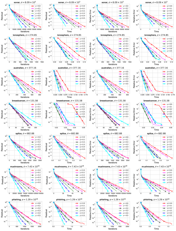
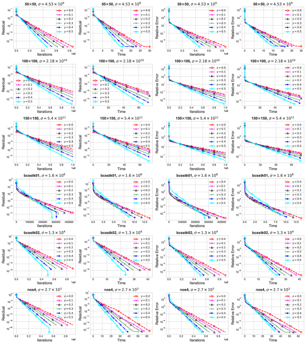
For the GK method, random test instances are generated as follows: vector $x\in\mathbb{R}^{n}$ and matrix $A\in\mathbb{R}^{m\times n}$ are taken as i.i.d $\mathcal{N}(0,1)$, then $b$ is set as $b=Ax$ (we maintain the consistency of the system that way). We also consider the following ten datasets for LIBSVM collection: sonar ($200\times 60$), ionosphere ($351\times 34$), australian ($690\times 14$), breastcancer ($683\times 10$), splice ($1000\times 60$), svmguide3 ($1,243\times 21$), mushrooms ($8124\times 112$), phishing ($11055\times 68$), a7a ($16,100\times 123$), a9a ($32,561\times 123$). The random instances of GCD method are generated as follows: we first generate Gaussian matrix $G\in\mathbb{R}^{m\times n}$ and vector $x$ and then set $A=G^{T}G,\ b=Ax$. For real dataset, we consider the following positive definite matrices from the SuiteSparse Matrix collection: bcsstk01 ($48\times 48$), bcsstk02 ($66\times 66$), nos4 ($100\times 100$). For both of these algorithms, we measure residual error ($\|Ax_{k}-b\|_{2}$) and relative error $\|x_{k}-x^{*}\|_{B}/\|x_{0}-x^{*}\|_{B}$ 888We set $x^{*}=x_{0}+A^{\dagger}(b-Ax_{0})$, when $Ax=b$ has a unique solution $x^{*}=x_{int}$, where $x_{int}$ is the initial Gaussian vector used to generate $b$. with respect to the number of iterations and CPU time measured by MATLAB tic-toc function. The rest of the section is divided into two subsections. In subsection 7.1, we compare the proposed sampling rules. In subsection 7.2, we discuss the effect of momentum on the greedy algorithms.

7.1 Comparison among Sampling Rules without Momentum

In this subsection, we perform comparison experiments for both methods with respect to the proposed sampling rules.

Refer to caption
Figure 1: GK: sampling rules comparison on random data, left 2 panels: residual error vs No. of iterations and time, right 2 panels: relative error vs No. of iterations and time.
Refer to caption
Figure 2: GK: sampling rules comparison on LIBSVM data, left 2 panels: residual error vs No. of iterations and time, right 2 panels: relative error vs No. of iterations and time.
Refer to caption
Figure 3: GCD: sampling rules comparison on random and real data, left 2 panels: residual error vs No. of iterations and time, right 2 panels: relative error vs No. of iterations and time.

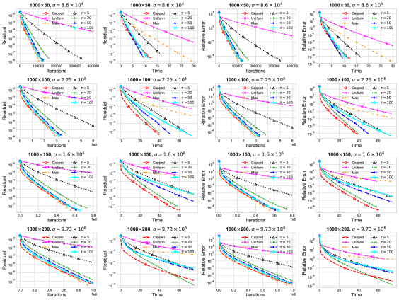
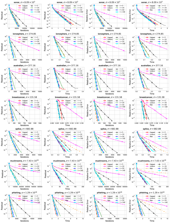
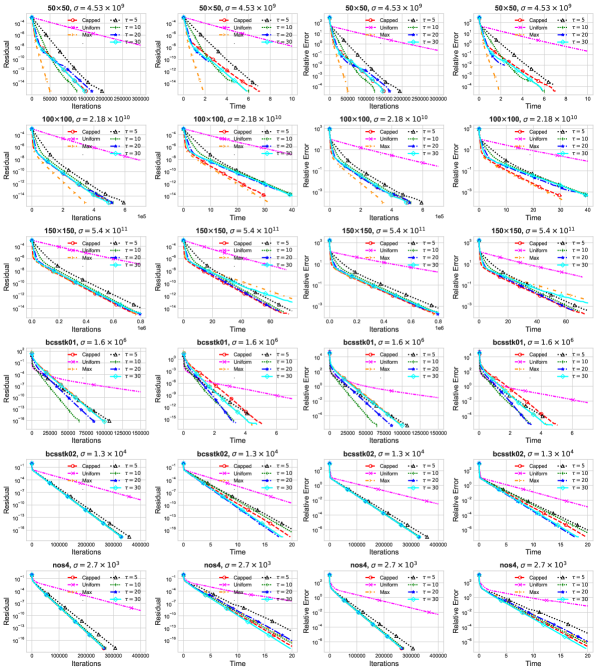
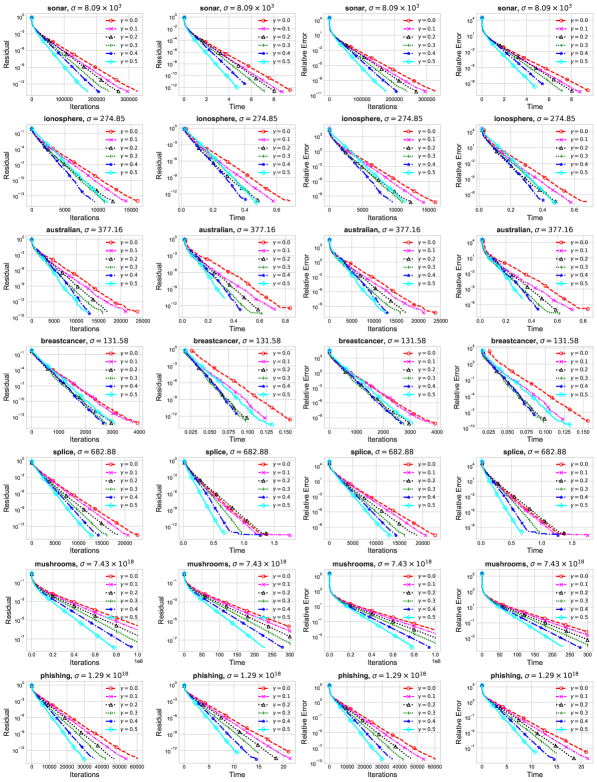
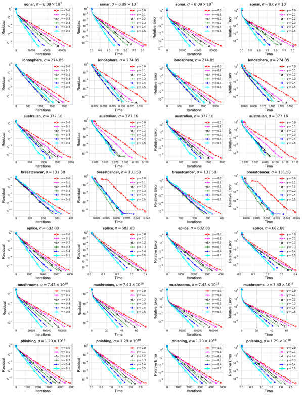
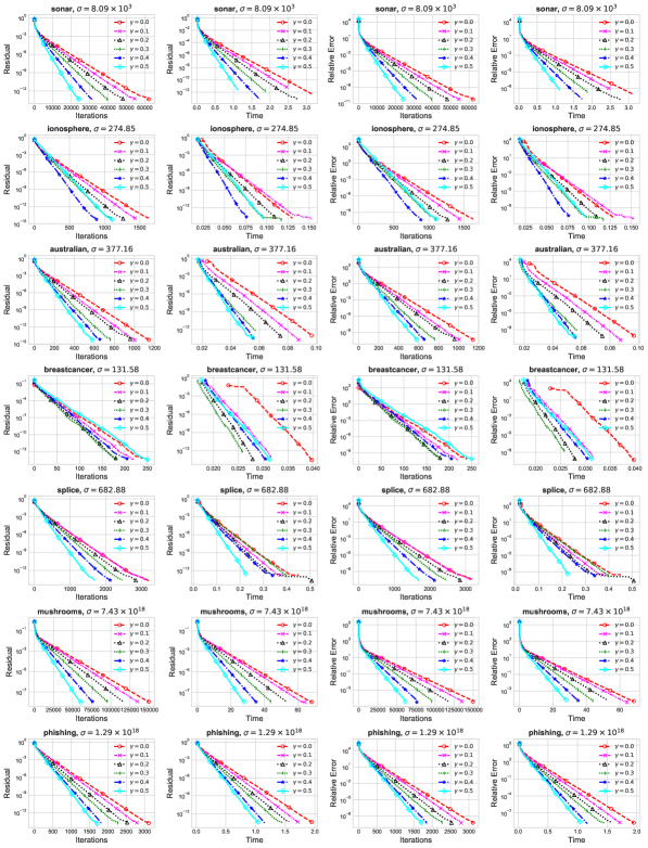
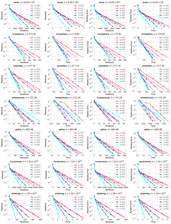
We choose the following sampling rules (1) GK method: uniform ($\tau=1$), $\tau=5$, $\tau=20$, $\tau=50$, $\tau=100$, max. distance ($\tau=m$), capped ($\tau_{1}=1,\tau_{2}=m,\theta=0.5$), and (2) GCD method: uniform ($\tau=1$), $\tau=5$, $\tau=10$, $\tau=20$, $\tau=30$, max. distance ($\tau=m$), capped ($\tau_{1}=1,\tau_{2}=m,\theta=0.5$). We compare the sampling rules on 7 LIBSVM problems for the GK method, on 6 random/real problems for the GCD method. In Figures 1, 2 and 3, we plot the performance measures of the selected sampling rules for GK and GCD method, respectively. From the figures, it can be concluded that the proposed greedy sampling rules heavily outperform existing sampling rules such as uniform and max. distance rules for both GK and GCD. Overall, the uniform sampling rule has the worst performance compared to other sampling rules. Moreover, the greedy methods performs equally compared to each other (in the next subsection, we elaborate this point in more detail, also see the Appendix section for more comparison graphs).

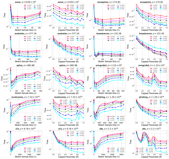
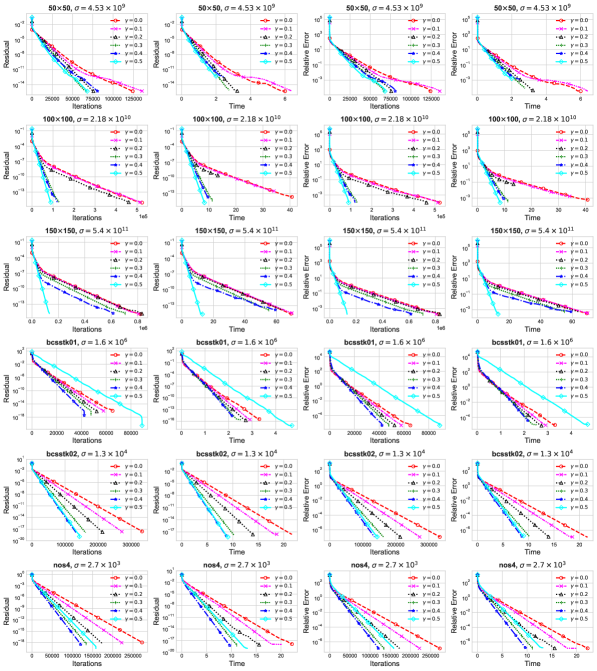
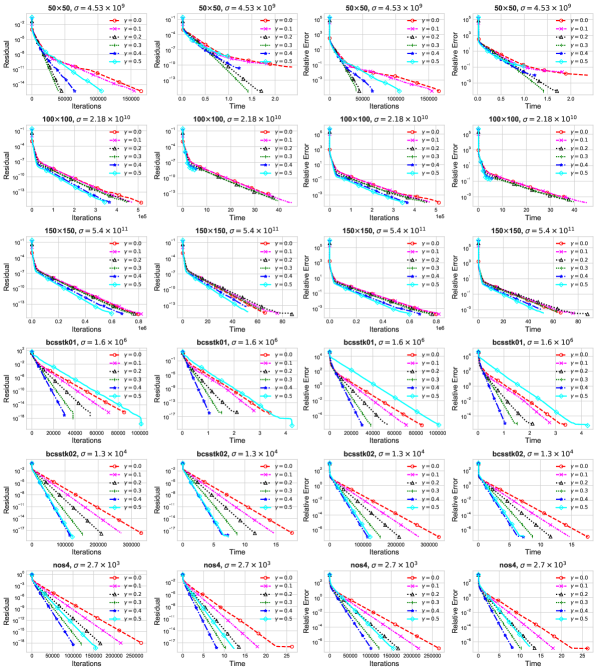
7.2 Comparison among Sampling Rules with Momentum

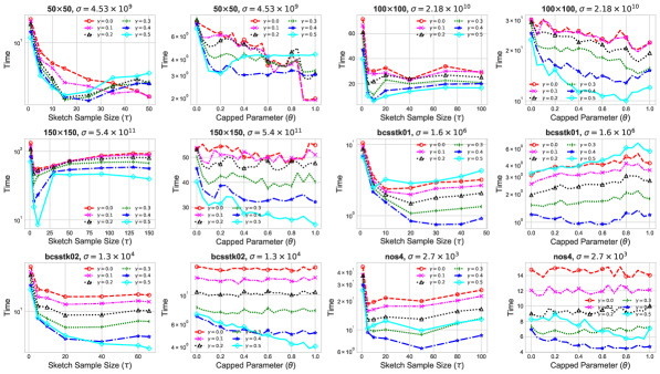
First, we discuss the effect of momentum parameter $\gamma$ on the choice of greedy sampling parameter selection, i.e., $\tau$ and $\theta$. In Figures 4 and 5, we plot the total CPU time taken by the momentum algorithms to reach a certain residual error threshold with varying $\tau$ and $\theta$. Here, we consider 10 LIBSVM problems for the GK method and 6 random/sparse problems for the GCD method. From the figures, it is evident that sample size $\tau$ has significant impact on the performance of momentum algorithms, whereas the effect of $\theta$ remains more or less constant for both methods. The choice $1<\tau\ll m$ produces the best performing methods that confirms our claim about the importance of sampling. Furthermore, the proposed momentum variants heavily outperform the basic methods with no momentum. Since, sampling plays an important role, in the following we compare the momentum algorithms for fixed $\tau$.

Refer to caption
Figure 4: GCD momentum (effect of sketch sample size $\tau$ and capped parameter $\theta$).

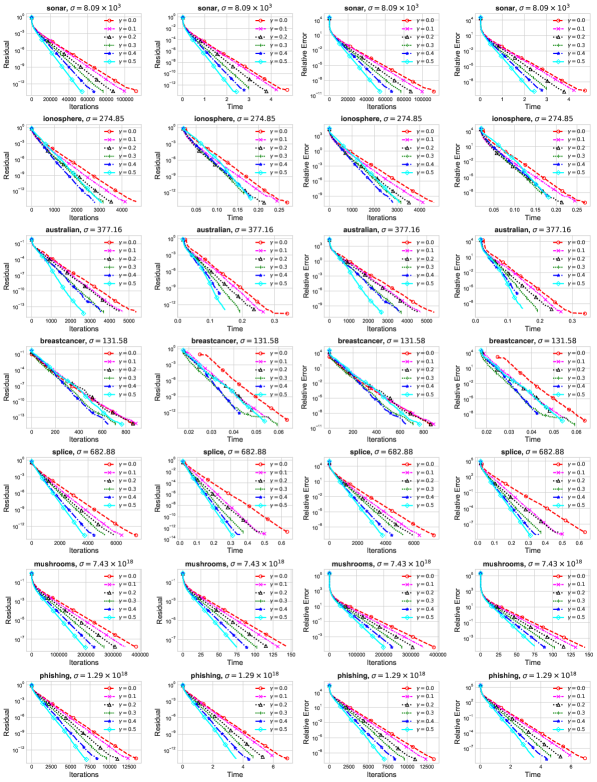
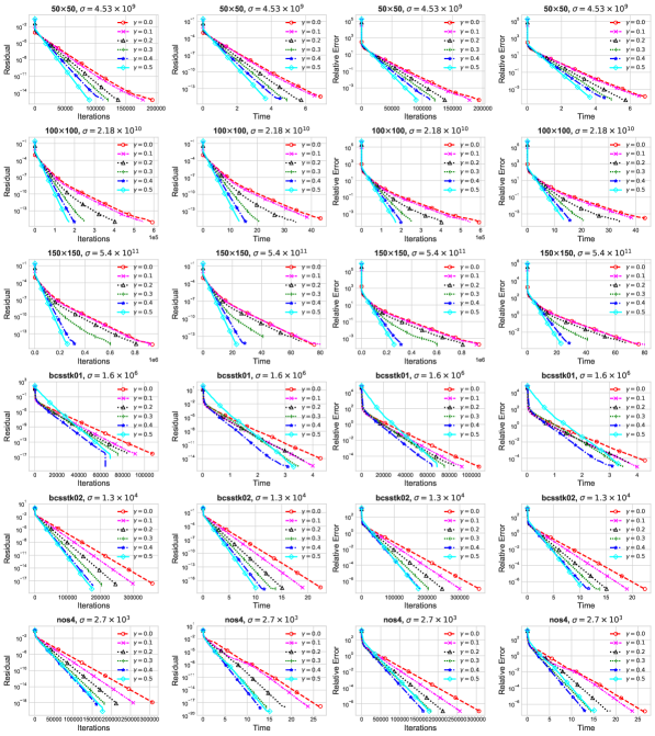
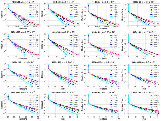
GK and GCD method with momentum

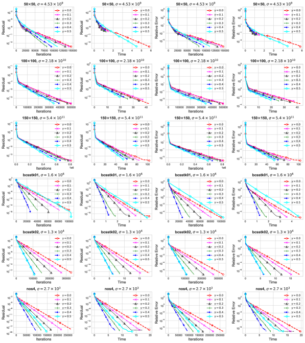
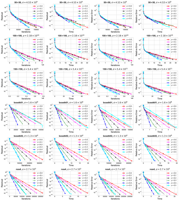
Here we compare the momentum algorithms for some fixed sampling rules. In Figures 6- 7, we plot the comparison graphs for GK and GCD method, respectively with $\tau=5$. From Figures 6 and 7, we see that the proposed momentum variants outperform the basic GK and GCD methods for all of the considered test instances (please see Figures 8-19 for different $\tau$ in the Appendix section). In the following, we summarise the findings of our numerical experiments:

Refer to caption
Figure 5: GK momentum (effect of sketch sample size $\tau$ and capped parameter $\theta$).
  • From our experiments, we find that the proposed greedy rules outperform the existing rules. For the case of greedy capped sampling, parameter $\theta$ has no significant impact on the algorithmic performance. However, for the greedy sketching rule, the choice of $\tau$ drives the performance and algorithms with sketch sample size $1<\tau\ll m$ have the best performance.

  • Over the course of our experiments, $\gamma$ is chosen arbitrarily. It is evident that the choice $\gamma=0.4$ leads to best performance in general. The choice $\gamma=0.5$ works well most of the times but fails significantly from time to time. $\gamma=0.4$ is the safe choice as it converges and has better performance.

  • We test the proposed methods on a wide range of random/real-world datasets. We find that, the proposed methods performs better on ill-conditional linear systems (condition number of data matrix $A$ is large). We report the corresponding condition numbers in the figures.

Refer to caption
Figure 6: GK with momentum (sketch Sample size, $\tau=5$): comparison among momentum variants on LIBSVM data, residual error and relative error vs CPU time and No. of iterations.
Refer to caption
Figure 7: GCD with momentum (sketch Sample size, $\tau=5$): comparison among momentum variants on Gaussian and Matrix market data, residual error and relative error vs CPU time and No. of iterations.

8 Conclusions

In this work, we propose a stochastic steepest descent framework for solving linear system of equations. Furthermore, we propose to incorporate greedy sketching strategies along with momentum technique to the basic method. In doing so, we synthesize well-known iterative methods such as steepest descent and randomized iterative methods such as randomized Kaczmarz, randomized co-ordinate descent into one framework. From our convergence analysis one can recover multiple convergence convergence results by varying sketching rules and sketching matrices. We validate the proposed algorithmic variants on a wide variety of datasets such as random Gaussian, LIBSVM, and matrix-market sparse matrices. From our numerical experiments, we conclude that the proposed sketching rule based methods heavily outperform the existing sketching rules. Moreover, the proposed momentum scheme accelerate algorithmic performance of the basic method. We conclude the paper with the following research query: we propose a connection between randomized iterative methods with iterative methods for solving linear system, one could ask if there exists a randomized scheme based on the SSDM method that will synthesize the well-known Conjugate Gradient into an equivalent randomized iterative method framework. Another possible extension would be to develop extensions of the proposed greedy sketching rules based on adaptive sketch sample size, i.e., $\tau_{k}$.

Appendix

Lemma 20

(Lemma 2.1 in (De Loera et al., 2017)) Let $\{x_{k}\},\ \{y_{k}\}$ be real non-negative sequences such that $x_{k+1}>x_{k}>0$ and $y_{k+1}\geq y_{k}\geq 0$, then

$\displaystyle\sum\limits_{k=1}^{n}x_{k}y_{k}\ \geq\ \sum\limits_{k=1}^{n}\overline{x}y_{k},\quad\text{where}\ \ \overline{x}=\frac{1}{n}\sum\limits_{k=1}^{n}x_{k}.$
Lemma 21

((Strang, 1960)) For any matrix $M\succ 0$, we have the following bound:

$\displaystyle\|u\|^{2}_{M}\|v\|^{2}_{M^{-1}}\leq\frac{\left[\lambda_{\max}(M)+\lambda_{\min}(M)\right]^{2}}{4\lambda_{\min}(M)\lambda_{\max}(M)}\|u\|^{2}\|v\|^{2}$

for all $u,v\in\mathbb{R}^{n}$ and this is the best bound possible.

Lemma 22

(Lemma 14 in (Gower et al., 2019b)) If the relation $\textbf{Null}(P)\subset\textbf{Null}(M^{T})$ holds for some matrix $M$ and positive semi-definite matrix $P\succeq 0$. Then, we have

$\displaystyle\textbf{Null}(M)=\textbf{Null}(M^{T}PM),\quad\textbf{Range}(M^{T})=\textbf{Range}(M^{T}PM)$

A Proofs

Proof  (Lemma 3) From the optimization problem (1), we find that

$\displaystyle x^{*}=-G^{-1}A^{T}\lambda\in\textbf{Range}(G^{-1}A^{T})$

for some $\lambda\in\mathbb{R}^{m}$. From the definition, $x_{0}\in\textbf{Range}(G^{-1}A^{T})$. Thus $r_{0}\in\textbf{Range}(G^{-\frac{1}{2}}A^{T})$. Now, assume that this identity holds for the first $k$ iterates. i.e.,

$\displaystyle r_{k-1}\in\textbf{Range}(G^{-\frac{1}{2}}A^{T}),\quad r_{k}\in\textbf{Range}(G^{-\frac{1}{2}}A^{T})$

Now, from the momentum update formula, we have the following:

$\displaystyle r_{k+1}=r_{k}-\omega\underbrace{G^{-\frac{1}{2}}A^{T}H(Ax-b)}_{\in\ \textbf{Range}(G^{-\frac{1}{2}}A^{T})}+\gamma\underbrace{(r_{k}-r_{k-1})}_{\in\ \textbf{Range}(G^{-\frac{1}{2}}A^{T})}$

Which implies $r_{k+1}\in\textbf{Range}(G^{-\frac{1}{2}}A^{T})$. This proves the first part. Note, that

$\displaystyle\textbf{Null}(\mathbf{T})=\textbf{Null}\left(G^{-\frac{1}{2}}A^{T}\sum\limits_{i=1}^{q}H_{i}AG^{-\frac{1}{2}}\right)=\textbf{Null}\left(A^{T}\sum\limits_{i=1}^{q}H_{i}AG^{-\frac{1}{2}}\right)=\textbf{Null}\left(AG^{-\frac{1}{2}}\right)$

in the last equality, we used Lemma 22 with $P=\sum\nolimits_{i=1}^{q}H_{i},\ M=A$. Taking orthogonal complement, we have the required relation.  

Proof  (Lemma 4)

We will first prove the first three identities. The upper bounds of (24), (25), and (27) follows from the fact that $T_{i_{k}}$ and $\operatorname{\mathbb{E}}[T]$ are positive semi-definite matrices. Note that, as $T_{i_{k}}^{\frac{1}{2}}r_{k}\in\textbf{Range}(T_{i_{k}}^{\frac{1}{2}})$, by the Courant-Fisher Theorem, we have the lower bound of (24). Similarly the lower bound of (25) follows from the fact that $T_{i_{k}}r_{k}\in\textbf{Range}(G^{-\frac{1}{2}}Z_{i_{k}}^{\frac{1}{2}})$. These arguments prove the first two identities of the Lemma. Now we have,

$\displaystyle\frac{1}{\mu_{2}}\leq\frac{1}{\mu_{2}(i_{k})}\leq\alpha_{i_{k}}=\frac{r_{k}^{T}T^{2}_{i_{k}}r_{k}}{r_{k}^{T}T^{3}_{i_{k}}r_{k}}\leq\frac{1}{\mu^{+}_{1}(i_{k})}\leq\frac{1}{\mu^{+}_{1}}$ (44)

Furthermore, with the choice $G=B$, we get $T^{2}_{i_{k}}=T_{i_{k}}$. That implies $\alpha_{i_{k}}=1$. This proves the Lemma.  

Proof  (Theorem 5) Using the definition of expectation from (20), we have

$\displaystyle\operatorname{\mathbb{E}}_{i}[f_{i}(x_{k})]$ $\displaystyle=\frac{1}{2\binom{q}{\tau}}\sum\limits_{j=0}^{q-\tau}\binom{\tau-1+j}{\tau-1}\|x_{k}-x^{*}\|_{Z_{\underline{\mathbf{i_{j}}}}}^{2}\leq\frac{\binom{q-1}{\tau-1}}{2\binom{q}{\tau}}\sum\limits_{j=0}^{q-\tau}r_{k}^{T}T_{\underline{\mathbf{i_{j}}}}r_{k}$
$\displaystyle\leq\frac{\tau}{2q}\sum\limits_{j=1}^{q}r_{k}^{T}T_{j}r_{k}=\frac{\tau}{2q}r_{k}^{T}\mathbf{T}r_{k}\leq\frac{\tau\lambda_{\max}\left(\mathbf{T}\right)}{2q}\|r_{k}\|^{2}$ (45)

Furthermore, the following holds

$\displaystyle\operatorname{\mathbb{E}}_{i}[f_{i}(x_{k})]$ $\displaystyle=\frac{1}{\binom{q}{\tau}}\sum\limits_{j=0}^{q-\tau}\binom{\tau-1+j}{\tau-1}f_{\underline{\mathbf{i_{j}}}}(x_{k})\leq\max_{i\in\{1,2,...,q\}}f_{i}(x_{k})\frac{1}{\binom{q}{\tau}}\sum\limits_{j=0}^{q-\tau}\binom{\tau-1+j}{\tau-1}$
$\displaystyle=\frac{1}{2}\max_{i\in\{1,2,...,q\}}r_{k}T_{i}r_{k}\leq\frac{\max_{i\in\{1,2,...,q\}}\mu_{2}(i)}{2}\|r_{k}\|^{2}\leq\frac{\mu_{2}}{2}\|r_{k}\|^{2}$ (46)

here, we used column-sum property of Pascal’s triangle, i.e., $\sum\nolimits_{j=0}^{q-\tau}\binom{\tau-1+j}{\tau-1}=\binom{q}{\tau}$. Combining (A) and (A), we get the upper bound of the proposed Lemma. Similarly, we have

$\displaystyle\operatorname{\mathbb{E}}_{i}$ [fi(xk)]=12(qτ)j=0qτ(τ1+jτ1)xkxZ𝐢𝐣¯2Lemma2012(qτ)j=0qτl=0qτ(τ1+lτ1)qτ+1xkxZ𝐢𝐣¯2delimited-[]subscript𝑓𝑖subscript𝑥𝑘12binomial𝑞𝜏superscriptsubscript𝑗0𝑞𝜏binomial𝜏1𝑗𝜏1superscriptsubscriptnormsubscript𝑥𝑘superscript𝑥subscript𝑍¯subscript𝐢𝐣2Lemma2012binomial𝑞𝜏superscriptsubscript𝑗0𝑞𝜏superscriptsubscript𝑙0𝑞𝜏binomial𝜏1𝑙𝜏1𝑞𝜏1superscriptsubscriptnormsubscript𝑥𝑘superscript𝑥subscript𝑍¯subscript𝐢𝐣2\displaystyle[f_{i}(x_{k})]=\frac{1}{2\binom{q}{\tau}}\sum\limits_{j=0}^{q-\tau}\binom{\tau-1+j}{\tau-1}\|x_{k}-x^{*}\|_{Z_{\underline{\mathbf{i_{j}}}}}^{2}\overset{\text{Lemma}\ \ref{lem:skmseq}}{\geq}\frac{1}{2\binom{q}{\tau}}\sum\limits_{j=0}^{q-\tau}\frac{\sum\limits_{l=0}^{q-\tau}\binom{\tau-1+l}{\tau-1}}{q-\tau+1}\|x_{k}-x^{*}\|_{Z_{\underline{\mathbf{i_{j}}}}}^{2}
$\displaystyle=\frac{1}{2(q-\tau+1)}\sum\limits_{j=0}^{q-\tau}\|x_{k}-x^{*}\|_{Z_{\underline{\mathbf{i_{j}}}}}^{2}\geq\frac{1}{2(q-\tau+1)}\min\left\{1,\frac{q-\tau+1}{q-s_{k}}\right\}\sum\limits_{j=1}^{q}\|x_{k}-x^{*}\|_{Z_{j}}$
$\displaystyle=\frac{1}{2\bar{q}_{k}}(x_{k}-x^{*})^{T}G^{\frac{1}{2}}\mathbf{T}G^{\frac{1}{2}}(x_{k}-x^{*})\geq\frac{\lambda_{\min}^{+}\left(\mathbf{T}\right)}{2\bar{q}_{k}}\|r_{k}\|^{2}$ (47)

the last inequality follows from Lemma 3 along with the Courant-Fisher theorem. Similarly, for the capped rule, we have

$\displaystyle\operatorname{\mathbb{E}}[f_{i}(x)\ |\ i\sim\mathcal{C}(\theta,\tau_{1},\tau_{2})]$ $\displaystyle=\sum\limits_{j\in\mathcal{W}}p_{j}f_{j}(x)\geq\theta\operatorname{\mathbb{E}}[f_{j}(x)\ |\ j\sim\mathcal{G}(\tau_{1})]+(1-\theta)\operatorname{\mathbb{E}}[f_{j}(x)\ |\ j\sim\mathcal{G}(\tau_{2})]$
$\displaystyle\geq\theta\frac{\lambda_{\min}^{+}\left(\mathbf{T}\right)}{2\bar{q}_{k}(\tau_{1})}\|r_{k}\|^{2}+(1-\theta)\frac{\lambda_{\min}^{+}\left(\mathbf{T}\right)}{2\bar{q}_{k}(\tau_{2})}\|r_{k}\|^{2}.$ (48)

Similarly, we have

$\displaystyle\operatorname{\mathbb{E}}[f_{i}(x)\ |\ i\sim\mathcal{C}(\theta,\tau_{1},\tau_{2})]=\sum\limits_{j\in\mathcal{W}}p_{j}f_{j}(x)\leq\max_{i\in\{1,2,...,q\}}f_{i}(x)\leq\frac{\mu_{2}}{2}\|r_{k}\|^{2}.$ (49)

Combining (A) and (49), we get the required result.  

Proof  (Theorem 7) To prove the bound of (32), we use the Cauchy-Swartrz inequality, i.e,

$\displaystyle(r_{k}^{T}T^{2}_{i_{k}}r_{k})^{2}\leq\|T_{i_{k}}^{\frac{1}{2}}r_{k}\|^{2}\|T_{i_{k}}^{\frac{3}{2}}r_{k}\|^{2}=(r_{k}^{T}T_{i_{k}}r_{k})(r_{k}^{T}T^{3}_{i_{k}}r_{k})$ (50)

Since, $T_{i_{k}}\succeq 0$, the relation $\mu_{1}(i_{k})\|r_{k}\|^{2}\leq r_{k}^{T}T_{i_{k}}r_{k}\leq\mu_{2}(i_{k})\|r_{k}\|^{2}$ holds. Now, let’s denote

$\displaystyle\mathcal{H}(r_{k})=(\mu_{1}(i_{k})+\mu_{2}(i_{k}))r_{k}^{T}T_{i_{k}}r_{k}-r_{k}^{T}T^{2}_{i_{k}}r_{k}-\mu_{1}(i_{k})\mu_{2}(i_{k})\|r_{k}\|^{2}$

Note that, considering the given conditions we can check that $\mathcal{H}(r_{k})\geq 0$ holds for all $k\geq 1$. Then, we have the following:

$\displaystyle(r_{k}^{T}T^{2}_{i_{k}}r_{k})\|r_{k}\|^{2}-(r_{k}^{T}T_{i_{k}}r_{k})^{2}$ $\displaystyle=\left(r_{k}^{T}T_{i_{k}}r_{k}-\mu_{1}(i_{k})\|r_{k}\|^{2}\right)\left(\mu_{2}(i_{k})\|r_{k}\|^{2}-r_{k}^{T}T_{i_{k}}r_{k}\right)-\|r_{k}\|^{2}\mathcal{H}(r_{k})$
$\displaystyle\leq\|r_{k}\|^{4}\left(\frac{r_{k}^{T}T_{i_{k}}r_{k}}{\|r_{k}\|^{2}}-\mu_{1}(i_{k})\right)\left(\mu_{2}(i_{k})-\frac{r_{k}^{T}T_{i_{k}}r_{k}}{\|r_{k}\|^{2}}\right)$
$\displaystyle\leq\|r_{k}\|^{4}\ \frac{[\mu_{2}(i_{k})-\mu_{1}(i_{k})]^{2}}{4}$ (51)

where, the last inequality follows from the fact that $\mu_{1}(i_{k})\leq r_{k}^{T}T_{i_{k}}r_{k}/\|r_{k}\|^{2}\leq\mu_{2}(i_{k})$ holds. Now, replacing $r_{k}$ with $T_{i_{k}}^{\frac{1}{2}}r_{k}$ in equation (A) and simplifying further, we get

$\displaystyle\frac{(r_{k}^{T}T_{i_{k}}r_{k})(r_{k}^{T}T^{3}_{i_{k}}r_{k})}{(r_{k}^{T}T^{2}_{i_{k}}r_{k})^{2}}-1\leq\frac{[\mu_{2}(i_{k})-\mu_{1}(i_{k})]^{2}}{4}\frac{(r_{k}^{T}T_{i_{k}}r_{k})^{2}}{(r_{k}^{T}T^{2}_{i_{k}}r_{k})^{2}}\leq\frac{[\mu_{2}(i_{k})-\mu_{1}(i_{k})]^{2}}{4[\mu_{1}^{+}(i_{k})]^{2}}\leq\frac{\left(\sigma_{i_{k}}\right)^{2}}{4}$ (52)

where, the last inequality follows from the fact that $\mu_{1}(i_{k})\geq 0$. Combining (50) and (52), we get the result of (32) Now, assume $T_{i_{k}}\succ 0$ for each $i_{k}$. This implies $0<\mu_{1}(i_{k})=\mu_{1}^{+}(i_{k})$ and $T^{-1}(i_{k})$ exists for each $i_{k}\geq 1$. Now, denote $M=T_{i_{k}},\ u=T_{i_{k}}r_{k},\ v=T^{\frac{1}{2}}_{i_{k}}r_{k}$. Substituting the above parameter values in Lemma 21, we get the following:

$\displaystyle\frac{\|u\|^{2}_{M}\|v\|^{2}_{M^{-1}}}{\|u\|^{2}\|v\|^{2}}=\frac{\|T_{i_{k}}r_{k}\|^{2}_{T_{i_{k}}}\|T^{\frac{1}{2}}_{i_{k}}r_{k}\|^{2}_{T_{i_{k}}^{-1}}}{\|T_{i_{k}}r_{k}\|^{2}\|T^{\frac{1}{2}}_{i_{k}}r_{k}\|^{2}}=\frac{(r_{k}^{T}r_{k})(r_{k}^{T}T_{i_{k}}^{3}r_{k})}{(r_{k}^{T}T_{i_{k}}r_{k})(r_{k}^{T}T_{i_{k}}^{2}r_{k})}\leq\frac{[\mu_{2}(i_{k})+\mu_{1}(i_{k})]^{2}}{4\mu_{1}(i_{k})\mu_{2}(i_{k})}=\frac{\left(1+\sigma_{i_{k}}\right)^{2}}{4\sigma_{i_{k}}}$

this proves the bound of (33). In a similar fashion, take $M=T_{i_{k}},\ u=v=T_{i_{k}}r_{k}$ in Lemma 21. That gives us,

$\displaystyle\frac{\|u\|^{2}_{M}\|v\|^{2}_{M^{-1}}}{\|u\|^{2}\|v\|^{2}}=\frac{\|T_{i_{k}}r_{k}\|^{2}_{T_{i_{k}}}\|T_{i_{k}}r_{k}\|^{2}_{T_{i_{k}}^{-1}}}{\|T_{i_{k}}r_{k}\|^{4}}=\frac{(r_{k}^{T}T_{i_{k}}r_{k})(r_{k}^{T}T_{i_{k}}^{3}r_{k})}{(r_{k}^{T}T_{i_{k}}^{2}r_{k})^{2}}\leq\frac{[\mu_{2}(i_{k})+\mu_{1}(i_{k})]^{2}}{4\mu_{1}(i_{k})\mu_{2}(i_{k})}=\frac{\left(1+\sigma_{i_{k}}\right)^{2}}{4\sigma_{i_{k}}}$

This is precisely what we claimed in (34).  

Proof  (Theorem 9) From the update formula we have,

$\displaystyle x_{k+1}-x^{*}=x_{k}-x^{*}+\omega\alpha_{i_{k}}G^{-1}Z_{i_{k}}(x^{*}-x_{k})=\left(I-\omega\alpha_{i_{k}}G^{-1}Z_{i_{k}}\right)(x_{k}-x^{*})$

Taking expectation with respect to the index ${i_{k}}$, we get conditioned on $x_{k}$, we get,

$\displaystyle\operatorname{\mathbb{E}}_{i_{k}}\left[x_{k+1}-x^{*}\right]=\left(I-\omega G^{-1}\operatorname{\mathbb{E}}_{i_{k}}\left[\alpha_{i_{k}}Z_{i_{k}}\right]\right)(x_{k}-x^{*})$

Taking expectation again and using tower property we get

$\displaystyle\operatorname{\mathbb{E}}\left[x_{k+1}-x^{*}\right]=\operatorname{\mathbb{E}}\left[\operatorname{\mathbb{E}}_{i_{k}}\left[x_{k+1}-x^{*}\right]\right]$ $\displaystyle=\operatorname{\mathbb{E}}\left[\left(I-\omega G^{-1}\operatorname{\mathbb{E}}_{i_{k}}\left[\alpha_{i_{k}}Z_{i_{k}}\right]\right)(x_{k}-x^{*})\right]$
$\displaystyle=\left(I-\omega G^{-1}\operatorname{\mathbb{E}}_{i_{k}}\left[\alpha_{i_{k}}Z_{i_{k}}\right]\right)\operatorname{\mathbb{E}}\left[x_{k}-x^{*}\right]$

Taking $G-$ norm in both sides, we get the following

$\displaystyle\big{\|}\operatorname{\mathbb{E}}\left[x_{k+1}-x^{*}\right]\big{\|}_{G}^{2}$ $\displaystyle=\big{\|}\left(I-\omega G^{-1}\operatorname{\mathbb{E}}_{i_{k}}\left[\alpha_{i_{k}}Z_{i_{k}}\right]\right)\operatorname{\mathbb{E}}\left[x_{k}-x^{*}\right]\big{\|}_{G}^{2}$
$\displaystyle\leq\big{\|}I-\omega G^{-1}\operatorname{\mathbb{E}}_{i_{k}}\left[\alpha_{i_{k}}Z_{i_{k}}\right]\big{\|}_{G}^{2}\big{\|}\operatorname{\mathbb{E}}\left[x_{k}-x^{*}\right]\big{\|}_{G}^{2}$

Now, from the definition of $G-$ norm we get

$\displaystyle\big{\|}I-\omega G^{-1}$ $\displaystyle\operatorname{\mathbb{E}}_{i_{k}}[\alpha_{i_{k}}Z_{i_{k}}]\big{\|}_{G}^{2}=\max_{\|G^{\frac{1}{2}}u\|_{2}=1}\big{\|}\left(I-\omega G^{-1}\operatorname{\mathbb{E}}_{i_{k}}\left[\alpha_{i_{k}}Z_{i_{k}}\right]\right)u\big{\|}_{2}^{2}$
$\displaystyle=\max_{\|v\|_{2}=1}\big{\|}\left(I-\omega G^{-\frac{1}{2}}\operatorname{\mathbb{E}}_{i_{k}}\left[\alpha_{i_{k}}Z_{i_{k}}\right]G^{-\frac{1}{2}}\right)v\big{\|}_{2}^{2}=\lambda_{\max}^{2}\left(I-\omega\operatorname{\mathbb{E}}_{i_{k}}\left[\alpha_{i_{k}}T_{i_{k}}\right]\right)$

This proves the Theorem.  

Proof  (Theorem 11) Take, $r_{k}=G^{\frac{1}{2}}(x_{k}-x^{*})$. Then from the update formula we get the following:

$\displaystyle\|r_{k+1}\|^{2}$ $\displaystyle=\big{\langle}\left(I-\omega\alpha_{i_{k}}G^{-1}Z_{i_{k}}\right)(x_{k}-x^{*}),\left(I-\omega\alpha_{i_{k}}G^{-1}Z_{i_{k}}\right)(x_{k}-x^{*})\big{\rangle}_{G}$
$\displaystyle=\Big{\langle}\left(I-\omega\alpha_{i_{k}}G^{-\frac{1}{2}}Z_{i_{k}}G^{-\frac{1}{2}}\right)r_{k},\left(I-\omega\alpha_{i_{k}}G^{-\frac{1}{2}}Z_{i_{k}}G^{-\frac{1}{2}}\right)r_{k}\Big{\rangle}=r_{k}^{T}\left(I-\omega\alpha_{i_{k}}T_{i_{k}}\right)^{2}r_{k}$

Now, using the expression of $\alpha_{i_{k}}$ we have the following:

$\displaystyle r_{k}^{T}\left(I-\omega\alpha_{i_{k}}T_{i_{k}}\right)^{2}r_{k}$ $\displaystyle=\|r_{k}\|^{2}-2\omega\alpha_{i_{k}}r_{k}^{T}T_{i_{k}}r_{k}+\omega^{2}\alpha^{2}_{i_{k}}r_{k}^{T}T^{2}_{i_{k}}r_{k}$
$\displaystyle=\|r_{k}\|^{2}-2\omega\frac{(r_{k}^{T}T_{i_{k}}r_{k})(r_{k}^{T}T^{2}_{i_{k}}r_{k})}{r_{k}^{T}T^{3}_{i_{k}}r_{k}}+\omega^{2}\frac{(r_{k}^{T}T^{2}_{i_{k}}r_{k})^{3}}{(r_{k}^{T}T^{3}_{i_{k}}r_{k})^{2}}$
$\displaystyle=\|r_{k}\|^{2}-\frac{(r_{k}^{T}T_{i_{k}}r_{k})(r_{k}^{T}T^{2}_{i_{k}}r_{k})}{r_{k}^{T}T^{3}_{i_{k}}r_{k}}\left(2\omega-\omega^{2}\frac{(r_{k}^{T}T^{2}_{i_{k}}r_{k})^{2}}{(r_{k}^{T}T^{3}_{i_{k}}r_{k})(r_{k}^{T}T_{i_{k}}r_{k})}\right)$
$\displaystyle\leq\|r_{k}\|^{2}-\frac{(r_{k}^{T}T_{i_{k}}r_{k})(r_{k}^{T}T^{2}_{i_{k}}r_{k})}{r_{k}^{T}T^{3}_{i_{k}}r_{k}}(2\omega-\omega^{2})$ (53)
$\displaystyle\leq\|r_{k}\|^{2}-(2\omega-\omega^{2})\frac{\|x_{k}-x^{*}\|^{2}_{Z_{i_{k}}}}{\mu_{2}}$ (54)

here, we used the bound for $\alpha_{i_{k}}$. Taking expectation in (54) we have the following

$\displaystyle\operatorname{\mathbb{E}}\left[\|r_{k+1}\|^{2}\ |\ i_{k}\sim\mathcal{R}\right]$ $\displaystyle\leq\|r_{k}\|^{2}-\frac{2(2\omega-\omega^{2})}{\mu_{2}}f(x_{k})\leq(1-\frac{(2\omega-\omega^{2})\lambda^{+}_{1}}{\mu_{2}})\|r_{k}\|^{2}$ (55)

Taking expectation again and using the tower property, we get the result when $T_{i_{k}}\succeq 0$. In the second part, we assumed $T_{i_{k}}\succ 0$, from (53) we have the following:

$\displaystyle\|r_{k}\|^{2}\left[1-(2\omega-\omega^{2})\frac{\|r_{k}\|^{2}_{T_{i_{k}}}\|r_{k}\|^{2}_{T^{2}_{i_{k}}}}{\|r_{k}\|^{2}\|r_{k}\|^{2}_{T^{3}_{i_{k}}}}\right]\leq\|r_{k}\|^{2}\left[1-(2\omega-\omega^{2})\frac{4\mu_{1}(i_{k})\mu_{2}(i_{k})}{\left[\mu_{2}(i_{k})+\mu_{1}(i_{k})\right]^{2}}\right]$ (56)

here, we used Lemma 21 with the choice $u=T^{\frac{1}{2}}_{i_{k}}r_{k}$ and $v=T_{i_{k}}r_{k}$. Now taking expectation with respect to index $i_{k}$ and considering (53) and (56), we get

$\displaystyle\operatorname{\mathbb{E}}\left[\|r_{k+1}\|^{2}\ |\ i_{k}\sim\mathcal{R}\right]$ $\displaystyle\leq\|r_{k}\|^{2}\left\{1-4(2\omega-\omega^{2})\operatorname{\mathbb{E}}\left[\frac{4\sigma_{i}}{\left(1+\sigma_{i}\right)^{2}}\right]\right\}$ (57)

Taking expectation again in (57) and using the tower property we get the result. Now, to prove the average iterate result, first note that from (55) we have the following:

$\displaystyle\frac{2(2\omega-\omega^{2})}{\mu_{2}}\sum\limits_{l=0}^{k-1}\operatorname{\mathbb{E}}[f(x_{k})]\leq\sum\limits_{l=0}^{k-1}\left(\operatorname{\mathbb{E}}[\|r_{k}\|^{2}]-\operatorname{\mathbb{E}}[\|r_{k+1}\|^{2}]\right)\leq\|r_{0}\|^{2}=\|x_{0}-x^{*}\|^{2}_{G}$ (58)

Therefore, we have

$\displaystyle\operatorname{\mathbb{E}}[\|\tilde{x}_{k}-x^{*}\|_{G}^{2}]$ $\displaystyle=\operatorname{\mathbb{E}}\left[\Big{\|}\frac{1}{k}\sum\limits_{l=1}^{k}\left(x_{l}-x^{*}\right)\Big{\|}^{2}_{G}\right]\leq\operatorname{\mathbb{E}}\left[\frac{1}{k}\sum\limits_{l=1}^{k}\big{\|}x_{l}-x^{*}\big{\|}^{2}_{G}\right]=\frac{1}{k}\sum\limits_{l=1}^{k}\operatorname{\mathbb{E}}[\|e_{l}\|^{2}]$
$\displaystyle\leq\frac{2}{k\lambda_{1}^{+}}\sum\limits_{l=1}^{k}\operatorname{\mathbb{E}}[f(x_{l})]\leq\frac{\mu_{2}\|x_{0}-x^{*}\|^{2}_{G}}{\omega k\lambda_{1}^{+}(2-\omega)}.$

This proves the average iterate result of Theorem 11.  

Proof  (Theorem 13) From the update formula, we have the following:

$\displaystyle\|x_{k+1}-x^{*}\|_{Z_{i_{k}}}^{2}$ $\displaystyle=\|x_{k}-x^{*}-\omega\alpha_{i_{k}}G^{-1}Z_{i_{k}}(x_{k}-x^{*})\|_{Z_{i_{k}}}^{2}$
$\displaystyle=\|x_{k}-x^{*}\|_{Z_{i_{k}}}^{2}-2\alpha_{i_{k}}r_{k}^{T}T_{i_{k}}r_{k}+\omega^{2}\alpha_{i_{k}}^{2}r_{k}^{T}T^{3}_{i_{k}}r_{k}$
$\displaystyle=\|x_{k}-x^{*}\|_{Z_{i_{k}}}^{2}-\alpha_{i_{k}}(2\omega-\omega^{2})r_{k}^{T}T^{2}_{i_{k}}r_{k}$ (59)

Now, the above identity can be simplified as follows:

$\displaystyle\frac{\|x_{k+1}-x^{*}\|_{Z_{i_{k}}}^{2}}{\|x_{k}-x^{*}\|_{Z_{i_{k}}}^{2}}=1-\frac{(2\omega-\omega^{2})(r_{k}^{T}T_{i_{k}}^{2}r_{k})^{2}}{(r_{k}^{T}T_{i_{k}}r_{k})(r_{k}^{T}T_{i_{k}}^{3}r_{k})}\leq 1-\frac{\mu^{+}_{1}(i_{k})(2\omega-\omega^{2})}{\mu_{2}(i_{k})}\leq 1-\frac{(2\omega-\omega^{2})}{\sigma_{i_{k}}}$ (60)

Similarly, considering (A) again and using (34), we get

$\displaystyle\frac{\|x_{k+1}-x^{*}\|_{Z_{i_{k}}}^{2}}{\|x_{k}-x^{*}\|_{Z_{i_{k}}}^{2}}=1-(2\omega-\omega^{2})\frac{(r_{k}^{T}T_{i_{k}}^{2}r_{k})^{2}}{(r_{k}^{T}T_{i_{k}}r_{k})(r_{k}^{T}T_{i_{k}}^{3}r_{k})}\leq 1-\frac{4(2\omega-\omega^{2})}{4+\sigma_{i_{k}}^{2}}$ (61)

Now, taking expectation in (60) and (61), then substituting the results in (A) we get,

$\displaystyle\operatorname{\mathbb{E}}\left[\frac{f_{i_{k}}(x_{k+1})}{f_{i_{k}}(x_{k})}\right]=\operatorname{\mathbb{E}}\left[\frac{\|x_{k+1}-x^{*}\|_{Z_{i_{k}}}^{2}}{\|x_{k}-x^{*}\|_{Z_{i_{k}}}^{2}}\right]\leq 1-\frac{4(2\omega-\omega^{2})}{\min\{4\operatorname{\mathbb{E}}[\sigma_{i}],4+\operatorname{\mathbb{E}}[\sigma_{i}^{2}]\}}$

this proves the first part of the Theorem. Now, if $T_{i_{k}}\succ 0$ for each $i_{k}$, then considering (A) along with (34), we get the following:

$\displaystyle\frac{\|x_{k+1}-x^{*}\|_{Z_{i_{k}}}^{2}}{\|x_{k}-x^{*}\|_{Z_{i_{k}}}^{2}}=1-(2\omega-\omega^{2})\frac{(r_{k}^{T}T_{i_{k}}^{2}r_{k})^{2}}{(r_{k}^{T}T_{i_{k}}r_{k})(r_{k}^{T}T_{i_{k}}^{3}r_{k})}\leq 1-\frac{4\sigma_{i_{k}}(2\omega-\omega^{2})}{\left(1+\sigma_{i_{k}}\right)^{2}}$ (62)

Taking expectation in (62), we get the required result. Since, we have the following bound

$\displaystyle\operatorname{\mathbb{E}}[f(x_{k+1})]=\frac{1}{2}r_{k+1}^{T}\operatorname{\mathbb{E}}[T]r_{k+1}\leq\frac{\lambda_{2}}{2}\ \|r_{k+1}\|^{2}$ (63)

Now, considering the first part results along with (63), we get the required bounds of the quantity $\operatorname{\mathbb{E}}[f(x_{k+1})]$. Furthermore, considering Jensen’s inequality along with (58), we get

$\displaystyle\operatorname{\mathbb{E}}[f(\tilde{x}_{k})]$ $\displaystyle\leq\operatorname{\mathbb{E}}\left[\frac{1}{k}\sum\limits_{l=1}^{k}f(x_{l})\right]=\frac{1}{k}\sum\limits_{l=1}^{k}\operatorname{\mathbb{E}}[f(x_{l})]\leq\frac{\mu_{2}\|x_{0}-x^{*}\|^{2}_{G}}{2\omega k(2-\omega)}.$

This proves the Theorem.  

Proof  (Theorem 15) From the update formula of the proposed momentum algorithm, we have,

$\displaystyle\|r_{k+1}\|^{2}=\|x_{k+1}-x^{*}\|^{2}_{G}$ $\displaystyle=\big{\|}x_{k}-\omega\alpha_{i_{k}}\ \nabla^{G}f_{i_{k}}(x_{k})+\gamma(x_{k}-x_{k-1})-x^{*}\big{\|}^{2}_{G}$
$\displaystyle=\underbrace{\big{\|}x_{k}-\omega\alpha_{i_{k}}\ \nabla^{G}f_{i_{k}}(x_{k})-x^{*}\big{\|}_{G}^{2}}_{M_{1}}+\gamma^{2}\underbrace{\|x_{k}-x_{k-1}\|_{G}^{2}}_{M_{2}}$
$\displaystyle+2\gamma\underbrace{\big{\langle}x_{k}-x^{*}\ ,\ x_{k}-x_{k-1}\big{\rangle}_{G}}_{M_{3}}-2\gamma\omega\underbrace{\alpha_{i_{k}}\big{\langle}\nabla^{G}f_{i_{k}}(x_{k})\ ,\ x_{k}-x_{k-1}\big{\rangle}_{G}}_{M_{4}}$
$\displaystyle=M_{1}+\gamma^{2}M_{2}+2\gamma M_{3}-2\gamma\omega M_{4}$

Here, we assume that at $k^{th}$ iteration, the sketching matrix matrix $S_{i_{k}}$ is chosen. Taking expectation with respect to index $i_{k}$, we get

$\displaystyle\operatorname{\mathbb{E}}_{i_{k}}[\|r_{k+1}\|^{2}]=\operatorname{\mathbb{E}}_{i_{k}}[M_{1}]+\gamma^{2}\operatorname{\mathbb{E}}_{i_{k}}[M_{2}]+2\gamma\operatorname{\mathbb{E}}_{i_{k}}[M_{3}]-2\gamma\omega\operatorname{\mathbb{E}}_{i_{k}}[M_{4}]$ (64)

Now, the first term of (64) can be simplified as follows:

$\displaystyle\operatorname{\mathbb{E}}_{i_{k}}[M_{1}]$ $\displaystyle=\operatorname{\mathbb{E}}_{i_{k}}\left[\big{\langle}\left(I-\omega\alpha_{i_{k}}G^{-1}Z_{i_{k}}\right)(x_{k}-x^{*}),\left(I-\omega\alpha_{i_{k}}G^{-1}Z_{i_{k}}\right)(x_{k}-x^{*})\big{\rangle}_{G}\right]$
$\displaystyle\leq\|r_{k}\|^{2}-\frac{2\omega(2-\omega)}{\mu_{2}}f(x_{k})$ (65)

We can simplify the second term of (64) as follows:

$\displaystyle\operatorname{\mathbb{E}}_{i_{k}}[M_{2}]=\|r_{k}-r_{k-1}\|^{2}\leq 2\|r_{k}\|^{2}+2\|r_{k-1}\|^{2}$ (66)

Now, we know the following parallelogram identity

$\displaystyle 2\langle u,v\rangle_{G}=\|u\|^{2}_{G}+\|v\|^{2}_{G}-\|u-v\|^{2}_{G}$ (67)

Take, $u=x_{k}-x^{*}$ and $v=x_{k}-x_{k-1}$. Then using the above identity we get,

$\displaystyle 2\operatorname{\mathbb{E}}_{i_{k}}[M_{3}]$ $\displaystyle=\big{\langle}x_{k}-x^{*},x_{k}-x_{k-1}\big{\rangle}_{G}=\|x_{k}-x^{*}\|^{2}_{G}+\|x_{k}-x_{k-1}\|^{2}_{G}-\|x_{k-1}-x^{*}\|^{2}_{G}$
$\displaystyle\leq 3\|x_{k}-x^{*}\|^{2}_{G}+\|x_{k-1}-x^{*}\|^{2}_{G}=3\|r_{k}\|^{2}+\|r_{k-1}\|^{2}$ (68)

Now, we need to simplify the fourth term of (64). Now, we can simplify $M_{4}$ as follows:

$\displaystyle M_{4}$ $\displaystyle=\alpha_{i_{k}}\big{\langle}GG^{-1}Z_{i_{k}}(x_{k}-x^{*})\ ,\ x_{k}-x_{k-1}\big{\rangle}$
$\displaystyle=\alpha_{i_{k}}\big{\langle}\nabla f_{i}(x_{k})\ ,\ x_{k}-x_{k-1}\big{\rangle}\geq\alpha_{i_{k}}f_{i}(x_{k})-\alpha_{i_{k}}f_{i}(x_{k-1})\geq\frac{f_{i}(x_{k})}{\mu_{2}}-\frac{f_{i}(x_{k-1})}{\mu^{+}_{1}}$

here, we used the convexity of the function $f_{i}(x)$. Now, the fourth term can be simplified as follows:

$\displaystyle 2\operatorname{\mathbb{E}}_{i_{k}}[M_{4}]\geq\frac{2f(x_{k})}{\mu_{2}}-\frac{2f(x_{k-1})}{\mu^{+}_{1}}$ (69)

Now, substituting the expressions of (A), (66), (A) and (69) in (64), we get

$\displaystyle\operatorname{\mathbb{E}}_{i_{k}}[\|r_{k+1}\|^{2}]$ $\displaystyle\leq(1+3\gamma+2\gamma^{2})\|r_{k}\|^{2}+(\gamma+2\gamma^{2})\|r_{k-1}\|^{2}+\frac{2\gamma\omega}{\mu^{+}_{1}}f(x_{k-1})-\frac{2\gamma\omega+4\omega-2\omega^{2}}{\mu_{2}}f(x_{k})$ (70)

Now, adding $\frac{2\zeta\omega}{\mu_{2}}f(x_{k})$ in both sides of (70), we get

$\displaystyle\operatorname{\mathbb{E}}_{i_{k}}[\|r_{k+1}\|^{2}$ $\displaystyle]+\frac{2\zeta\omega}{\mu_{2}}f(x_{k})\leq(1+3\gamma+2\gamma^{2})\|r_{k}\|^{2}+(\gamma+2\gamma^{2})\|r_{k-1}\|^{2}+\frac{2\gamma\omega}{\mu^{+}_{1}}f(x_{k-1})$
$\displaystyle-\frac{\left(2\gamma\omega+4\omega-2\omega^{2}-2\zeta\omega\right)}{\mu_{2}}f(x_{k})$
$\displaystyle\leq\left(1+3\gamma+2\gamma^{2}-\frac{\omega}{\mu_{2}}(\gamma+2-\omega-\zeta)\lambda^{+}_{1}\right)\|r_{k}\|^{2}+\left(\gamma+2\gamma^{2}\right)\|r_{k-1}\|^{2}$
$\displaystyle+\frac{2\xi\omega}{\mu^{+}_{1}}f(x_{k-1})+\frac{\left(2\gamma\omega-2\omega\xi\right)}{\mu^{+}_{1}}f(x_{k-1})$
$\displaystyle\leq\left(1+3\gamma+2\gamma^{2}-\frac{\omega}{\mu_{2}}(\gamma+2-\omega-\zeta)\lambda^{+}_{1}\right)\|r_{k}\|^{2}+\frac{2\xi\omega}{\mu^{+}_{1}}f(x_{k-1})$
$\displaystyle+\left(\gamma+2\gamma^{2}+\frac{\omega(\gamma-\xi)}{\mu^{+}_{1}}\lambda_{2}\right)\|r_{k-1}\|^{2}$
$\displaystyle=\phi_{1}\|r_{k}\|^{2}+\phi_{2}\|r_{k-1}\|^{2}+\frac{2\xi\omega}{\mu^{+}_{1}}f(x_{k-1})$ (71)

Here, we used the fact $\gamma\geq\max\left\{\xi,\zeta-2+\omega\right\}$. Taking expectation again in (A) and using the tower property, we get the following:

$\displaystyle\operatorname{\mathbb{E}}[\|r_{k+1}\|^{2}]+\frac{2\zeta\omega}{\mu_{2}}\operatorname{\mathbb{E}}[f(x_{k})]\leq\phi_{1}\operatorname{\mathbb{E}}[\|r_{k}\|^{2}]+\phi_{2}\operatorname{\mathbb{E}}[\|r_{k-1}\|^{2}]+\frac{2\xi\omega}{\mu^{+}_{1}}\operatorname{\mathbb{E}}[f(x_{k-1})]$ (72)

Now, the parameter $\delta$ satisfies the following relations:

$\displaystyle\xi\leq\frac{\zeta\mu^{+}_{1}(\delta+\phi_{1})}{\mu_{2}},\quad\text{and}\quad\phi_{2}\leq\delta(\delta+\phi_{1})$ (73)

Considering equations (72) and (73), we have the following:

$\displaystyle\operatorname{\mathbb{E}}\left[\mathcal{V}_{k+1}\right]$ $\displaystyle=\operatorname{\mathbb{E}}[\|r_{k+1}\|^{2}]+\delta\operatorname{\mathbb{E}}[\|r_{k}\|^{2}]+\frac{2\zeta\omega}{\mu_{2}}\operatorname{\mathbb{E}}[f(x_{k})]$
$\displaystyle\leq(\phi_{1}+\delta)\operatorname{\mathbb{E}}[\|r_{k}\|^{2}]+\phi_{2}\operatorname{\mathbb{E}}[\|r_{k-1}\|^{2}]+\frac{2\xi\omega}{\mu^{+}_{1}}\operatorname{\mathbb{E}}[f(x_{k-1})]$
$\displaystyle\leq(\phi_{1}+\delta)\operatorname{\mathbb{E}}[\|r_{k}\|^{2}]+\delta(\delta+\phi_{1})\operatorname{\mathbb{E}}[\|r_{k-1}\|^{2}]+\frac{2\omega\zeta(\delta+\phi_{1})}{\mu_{2}}\operatorname{\mathbb{E}}[f(x_{k-1})]$
$\displaystyle=(\phi_{1}+\delta)\left[\operatorname{\mathbb{E}}[\|r_{k}\|^{2}]+\delta\operatorname{\mathbb{E}}[\|r_{k-1}\|^{2}]+\frac{2\zeta\omega}{\mu_{2}}\operatorname{\mathbb{E}}[f(x_{k-1})]\right]=\rho\operatorname{\mathbb{E}}\left[\mathcal{V}_{k}\right]$ (74)

This proves the result. Finally, we have to show that $\rho<1$. Using the assumption $\phi_{1}+\phi_{2}<1$, we have

$\displaystyle\rho=\max\left\{\frac{\xi\mu_{2}}{\zeta\mu^{+}_{1}},\frac{\phi_{1}+\sqrt{\phi_{1}^{2}+4\phi_{2}}}{2}\right\}<\max\left\{1,\frac{\phi_{1}+\sqrt{\phi_{1}^{2}+4(1-\phi_{1})}}{2}\right\}=1$

This proves Theorem 15.  

Proof  (Theorem 17) First, let us define $\vartheta_{l}=\frac{\gamma}{1-\gamma}[x_{l}-x_{l-1}],\quad\chi_{l}=\|x_{l}+\vartheta_{l}-x^{*}\|_{G}^{2}$ for any natural number $l\geq 1$. Also assume that the sketching matrix $S_{i_{l}}$ is chosen at iteration $l$. Now, using the update formula of (14), we get

$\displaystyle\chi_{l+1}$ $\displaystyle=\|x_{l+1}+\vartheta_{l+1}-x^{*}\|_{G}^{2}=\big{\|}x_{l}+\vartheta_{l}-\frac{\omega\alpha_{i_{l}}}{1-\gamma}\nabla^{G}f_{i_{l}}(x_{l})-x^{*}\big{\|}_{G}^{2}$
$\displaystyle=\|x_{l}+\vartheta_{l}-x^{*}\|_{G}^{2}+\frac{\omega^{2}\alpha^{2}_{i_{l}}}{(1-\gamma)^{2}}\|\nabla^{G}f_{i_{l}}(x_{l})\|_{G}^{2}-\frac{2\omega\alpha_{i_{l}}}{1-\gamma}\big{\langle}x_{l}+\vartheta_{l}-x^{*}\ ,\ \nabla^{G}f_{i_{l}}(x_{l})\big{\rangle}_{G}$
$\displaystyle=\chi_{l}+\frac{2\omega^{2}}{(\mu^{+}_{1})^{2}(1-\gamma)^{2}}f_{i_{l}}(x_{l})-\frac{2\omega}{1-\gamma}\underbrace{\alpha_{i_{l}}\big{\langle}x_{l}+\vartheta_{l}-x^{*}\ ,\ \nabla^{G}f_{i_{l}}(x_{l})\big{\rangle}_{G}}_{J}.$ (75)

The third term can be simplified as follows:

$\displaystyle-\frac{2\omega}{1-\gamma}J$ $\displaystyle=-\frac{2\omega}{1-\gamma}\big{\langle}x_{l}-x^{*},\alpha_{i_{l}}Z_{i_{l}}(x_{l}-x^{*})\big{\rangle}+\frac{2\omega\gamma}{(1-\gamma)^{2}}\big{\langle}x_{l-1}-x_{l},\alpha_{i_{l}}Z_{i_{l}}(x_{l}-x^{*})\big{\rangle}$
$\displaystyle\leq-\frac{4\omega}{1-\gamma}\alpha_{i_{l}}f_{i}(x_{l})+\frac{2\omega\gamma}{(1-\gamma)^{2}}\alpha_{i_{l}}\left[f_{i}(x_{l-1})-f_{i}(x_{l})\right]$
$\displaystyle\leq-\frac{4\omega}{\mu_{2}(1-\gamma)}f_{i}(x_{l})+\frac{2\omega\gamma}{\mu^{+}_{1}(1-\gamma)^{2}}f_{i}(x_{l-1})-\frac{2\omega\gamma}{\mu_{2}(1-\gamma)^{2}}f_{i}(x_{l}).$ (76)

Taking expectation on both sides of A with respect to index $i_{l}$, we get

$\displaystyle\operatorname{\mathbb{E}}_{i_{l}}[\chi_{l+1}]$ $\displaystyle\leq\chi_{l}+\frac{2\omega^{2}f(x_{l})}{\mu_{2}^{2}(1-\gamma)^{2}}-\frac{2\omega\operatorname{\mathbb{E}}_{i_{l}}[J]}{1-\gamma}\leq\chi_{l}+\frac{2\omega\gamma f(x_{l-1})}{\mu^{+}_{1}(1-\gamma)^{2}}-\frac{2\omega\gamma f(x_{l})}{\mu^{+}_{1}(1-\gamma)^{2}}-\varpi f(x_{l})$ (77)

where, the constant $\varpi$ is taken as

$\displaystyle\varpi$ $\displaystyle=\frac{4\omega}{\mu_{2}(1-\gamma)}-\frac{2\omega^{2}}{\mu_{2}^{2}(1-\gamma)^{2}}+\frac{2\omega\gamma}{\mu_{2}(1-\gamma)^{2}}-\frac{2\omega\gamma}{\mu^{+}_{1}(1-\gamma)^{2}}=\frac{2\omega\left[2-\frac{\omega}{\mu_{2}}-\gamma\left(1+\frac{\mu_{2}}{\mu^{+}_{1}}\right)\right]}{\mu_{2}(1-\gamma)^{2}}>0.$

Simplifying equation (77) further, we get

$\displaystyle\operatorname{\mathbb{E}}_{i_{l}}[\chi_{l+1}]+\frac{2\omega\gamma}{\mu^{+}_{1}(1-\gamma)^{2}}f(x_{l})+\varpi f(x_{l})\ \leq\ \chi_{l}+\frac{2\omega\gamma}{\mu^{+}_{1}(1-\gamma)^{2}}f(x_{l-1}),$ (78)

Taking expectation again in (78) and using the tower property of expectation, we get the following recurrence

$\displaystyle y_{l+1}+\varpi\operatorname{\mathbb{E}}[f(x_{l})]\leq y_{l},\quad l=1,2,3...$ (79)

with the definition: $y_{l}=\operatorname{\mathbb{E}}[\chi_{l}]+\frac{2\omega\gamma}{\mu^{+}_{1}(1-\gamma)^{2}}\operatorname{\mathbb{E}}[f(x_{l-1})]$. Summing up (79) for $l\in[1,k]$, we have

$\displaystyle\sum\limits_{l=1}^{k}\operatorname{\mathbb{E}}[f(x_{l})]\ \leq\ \frac{y_{1}-y_{k+1}}{\varpi}\ \leq\ \frac{y_{1}}{\varpi}$ (80)

Furthermore, using the convexity property of function $f$, we get

𝔼[f(xk¯)]=𝔼[f(l=1kxlk)]𝔼[1kl=1kf(xl)]=1kl=1k𝔼[f(xl)](80)y1ϖk𝔼𝑓¯subscript𝑥𝑘𝔼𝑓superscriptsubscript𝑙1𝑘subscript𝑥𝑙𝑘𝔼1𝑘superscriptsubscript𝑙1𝑘𝑓subscript𝑥𝑙1𝑘superscriptsubscript𝑙1𝑘𝔼𝑓subscript𝑥𝑙italic-(80italic-)subscript𝑦1italic-ϖ𝑘\displaystyle\operatorname{\mathbb{E}}\left[f(\bar{x_{k}})\right]=\operatorname{\mathbb{E}}\left[f\left(\sum\limits_{l=1}^{k}\frac{x_{l}}{k}\right)\right]\ \leq\ \operatorname{\mathbb{E}}\left[\frac{1}{k}\sum\limits_{l=1}^{k}f(x_{l})\right]\ =\ \frac{1}{k}\sum\limits_{l=1}^{k}\operatorname{\mathbb{E}}[f(x_{l})]\ \overset{\eqref{ces:7}}{\leq}\frac{y_{1}}{\varpi k} (81)

From construction, we have $x_{0}=x_{1}$. Now, it can easily check that, $\vartheta_{1}=0$ and $\chi_{1}=\|x_{0}-x^{*}\|_{G}^{2}$. Therefore, from the definition of sequence $y_{1}$, we get

$\displaystyle y_{1}=\operatorname{\mathbb{E}}[\chi_{1}]+\frac{2\omega\gamma}{\mu^{+}_{1}(1-\gamma)^{2}}\operatorname{\mathbb{E}}[f(x_{0})]=\ \|x_{0}-x^{*}\|_{G}^{2}+\frac{2\omega\gamma}{\mu^{+}_{1}(1-\gamma)^{2}}f(x_{0}).$

Finally, substituting the values of $y_{1}$ and $\varpi$ in (81), we have the following

$\displaystyle\operatorname{\mathbb{E}}\left[f(\bar{x}_{k})\right]\leq\frac{\mu^{+}_{1}\mu_{2}(1-\gamma)^{2}\ \|x_{0}-x^{*}\|_{G}^{2}+2\gamma\omega\mu_{2}f(x_{0})}{2\omega k\left(2\mu^{+}_{1}\mu_{2}-\gamma\mu^{+}_{1}\mu_{2}-\gamma\mu_{2}^{2}-\omega\mu^{+}_{1}\right)}.$

This proves the Theorem.  

B Additional Experiments

Refer to caption
Figure 8: GK with momentum (sketch Sample size, $\tau=5$): comparison among momentum variants on Gaussian data, residual error and relative error vs CPU time and No. of iterations.
Refer to caption
Figure 9: GK with momentum (sketch Sample size, $\tau=1$): comparison among momentum variants on LIBSVM data, residual error and relative error vs CPU time and No. of iterations.
Refer to caption
Figure 10: GK with momentum (sketch Sample size, $\tau=20$): comparison among momentum variants on LIBSVM data, residual error and relative error vs CPU time and No. of iterations.
Refer to caption
Figure 11: GK with momentum (sketch Sample size, $\tau=50$): comparison among momentum variants on LIBSVM data, residual error and relative error vs CPU time and No. of iterations.
Refer to caption
Figure 12: GK with momentum (sketch Sample size, $\tau=m$): comparison among momentum variants on LIBSVM data, residual error and relative error vs CPU time and No. of iterations.
Refer to caption
Figure 13: GK with momentum (capped, $\theta=0.5,\tau_{1}=1,\tau_{2}=m$): comparison among momentum variants on LIBSVM data, residual error and relative error vs CPU time and No. of iterations.
Refer to caption
Figure 14: GCD with momentum (sketch Sample size, $\tau=1$): comparison among momentum variants on Gaussian and Matrix market data, residual error and relative error vs CPU time and No. of iterations.
Refer to caption
Figure 15: GCD with momentum (sketch Sample size, $\tau=10$): comparison among momentum variants on Gaussian and Matrix market data, residual error and relative error vs CPU time and No. of iterations.
Refer to caption
Figure 16: GCD with momentum (sketch Sample size, $\tau=20$): comparison among momentum variants on Gaussian and Matrix market data, residual error and relative error vs CPU time and No. of iterations.
Refer to caption
Figure 17: GCD with momentum (sketch Sample size, $\tau=30$): comparison among momentum variants on Gaussian and Matrix market data, residual error and relative error vs CPU time and No. of iterations.
Refer to caption
Figure 18: GCD with momentum (sketch Sample size, $\tau=m$): comparison among momentum variants on Gaussian and Matrix market data, residual error and relative error vs CPU time and No. of iterations.
Refer to caption
Figure 19: GCD with momentum (capped, $\theta=0.5,\tau_{1}=1,\tau_{2}=m$): comparison among momentum variants on Gaussian and Matrix market data, residual error and relative error vs CPU time and No. of iterations.

References

  • Abid and Gower (2018) Brahim Khalil Abid and Robert Gower. Stochastic algorithms for entropy-regularized optimal transport problems. In Amos Storkey and Fernando Perez-Cruz, editors, Proceedings of the Twenty-First International Conference on Artificial Intelligence and Statistics, volume 84 of Proceedings of Machine Learning Research, pages 1505–1512, Playa Blanca, Lanzarote, Canary Islands, 09–11 Apr 2018. PMLR. URL http://proceedings.mlr.press/v84/abid18a.html.
  • Agaskar et al. (2014) A. Agaskar, C. Wang, and Y. M. Lu. Randomized kaczmarz algorithms: Exact mse analysis and optimal sampling probabilities. In 2014 IEEE Global Conference on Signal and Information Processing (GlobalSIP), pages 389–393, Dec 2014. doi: 10.1109/GlobalSIP.2014.7032145.
  • Bai and Wu (2018a) Zhong-Zhi Bai and Wen-Ting Wu. On relaxed greedy randomized kaczmarz methods for solving large sparse linear systems. Applied Mathematics Letters, 83:21 – 26, 2018a. ISSN 0893-9659. doi: https://doi.org/10.1016/j.aml.2018.03.008. URL http://www.sciencedirect.com/science/article/pii/S0893965918300739.
  • Bai and Wu (2018b) Zhong-Zhi. Bai and Wen-Ting. Wu. On greedy randomized kaczmarz method for solving large sparse linear systems. SIAM Journal on Scientific Computing, 40(1):A592–A606, 2018b. doi: 10.1137/17M1137747. URL https://doi.org/10.1137/17M1137747.
  • Bengio et al. (2006) Yoshua Bengio, Olivier Delalleau, and Nicolas Le Roux. Label Propagation and Quadratic Criterion, pages 193–216. MIT Press, semi-supervised learning edition, January 2006. URL https://www.microsoft.com/en-us/research/publication/label-propagation-and-quadratic-criterion/.
  • Bhaya and Kaszkurewicz (2004) Amit Bhaya and Eugenius Kaszkurewicz. Steepest descent with momentum for quadratic functions is a version of the conjugate gradient method. Neural Networks, 17(1):65 – 71, 2004. ISSN 0893-6080. doi: https://doi.org/10.1016/S0893-6080(03)00170-9. URL http://www.sciencedirect.com/science/article/pii/S0893608003001709.
  • Briskman and Needell (2015) Jonathan Briskman and Deanna Needell. Block kaczmarz method with inequalities. J. Math. Imaging Vis., 52(3):385–396, July 2015. ISSN 0924-9907. doi: 10.1007/s10851-014-0539-7. URL https://doi.org/10.1007/s10851-014-0539-7.
  • Chi and Lu (2016) Y. Chi and Y. M. Lu. Kaczmarz method for solving quadratic equations. IEEE Signal Processing Letters, 23(9):1183–1187, 2016. doi: 10.1109/LSP.2016.2590468.
  • Csiba et al. (2015) Dominik Csiba, Zheng Qu, and Peter Richtárik. Stochastic dual coordinate ascent with adaptive probabilities. In Proceedings of the 32nd International Conference on International Conference on Machine Learning - Volume 37, ICML’15, page 674–683. JMLR.org, 2015.
  • Davis and Hu (2011) Timothy A. Davis and Yifan Hu. The university of florida sparse matrix collection. ACM Trans. Math. Softw., 38(1), December 2011. ISSN 0098-3500. doi: 10.1145/2049662.2049663. URL https://doi.org/10.1145/2049662.2049663.
  • De Loera et al. (2017) Jesús De Loera, Jamie Haddock, and Deanna Needell. A sampling kaczmarz–motzkin algorithm for linear feasibility. SIAM Journal on Scientific Computing, 39(5):S66–S87, 2017. doi: 10.1137/16M1073807. URL https://doi.org/10.1137/16M1073807.
  • Eldar and Needell (2011) Yonina C. Eldar and Deanna Needell. Acceleration of randomized kaczmarz method via the johnson–lindenstrauss lemma. Numerical Algorithms, 58(2):163–177, Oct 2011. ISSN 1572-9265. doi: 10.1007/s11075-011-9451-z. URL https://doi.org/10.1007/s11075-011-9451-z.
  • Gondzio (2013) Jacek Gondzio. Convergence analysis of an inexact feasible interior point method for convex quadratic programming. SIAM Journal on Optimization, 23(3):1510–1527, 2013. doi: 10.1137/120886017. URL https://doi.org/10.1137/120886017.
  • Gower et al. (2018) Robert Gower, Filip Hanzely, Peter Richtarik, and Sebastian U Stich. Accelerated stochastic matrix inversion: General theory and speeding up bfgs rules for faster second-order optimization. In S. Bengio, H. Wallach, H. Larochelle, K. Grauman, N. Cesa-Bianchi, and R. Garnett, editors, Advances in Neural Information Processing Systems 31, pages 1619–1629. Curran Associates, Inc., 2018. URL https://arxiv.org/abs/1802.04079.
  • Gower et al. (2019a) Robert Gower, Dmitry Kovalev, Felix Lieder, and Peter Richtarik. Rsn: Randomized subspace newton. In H. Wallach, H. Larochelle, A. Beygelzimer, F. dAlché Buc, E. Fox, and R. Garnett, editors, Advances in Neural Information Processing Systems, volume 32, pages 616–625. Curran Associates, Inc., 2019a. URL https://proceedings.neurips.cc/paper/2019/file/bc6dc48b743dc5d013b1abaebd2faed2-Paper.pdf.
  • Gower et al. (2019b) Robert Gower, Denali Molitor, Jacob Moorman, and Deanna Needell. Adaptive sketch-and-project methods for solving linear systems. 2019b.
  • Gower and Richtárik (2015) Robert M. Gower and Peter Richtárik. Randomized iterative methods for linear systems. SIAM Journal on Matrix Analysis and Applications, 36(4):1660–1690, 2015. doi: 10.1137/15M1025487. URL https://doi.org/10.1137/15M1025487.
  • Gower and Richtárik (2016) Robert M. Gower and Peter Richtárik. Linearly convergent randomized iterative methods for computing the pseudoinverse, 2016.
  • Gower and Richtárik (2017) Robert M. Gower and Peter. Richtárik. Randomized quasi-newton updates are linearly convergent matrix inversion algorithms. SIAM Journal on Matrix Analysis and Applications, 38(4):1380–1409, 2017. doi: 10.1137/16M1062053. URL https://doi.org/10.1137/16M1062053.
  • Gower et al. (2020) Robert M. Gower, Peter Richtárik, and Francis Bach. Stochastic quasi-gradient methods: variance reduction via jacobian sketching. Mathematical Programming, May 2020. ISSN 1436-4646. doi: 10.1007/s10107-020-01506-0. URL https://doi.org/10.1007/s10107-020-01506-0.
  • Haddock and Ma (2020) Jamie Haddock and Anna Ma. Greed works: An improved analysis of sampling kaczmarz-motzkin. arXiv preprint arXiv:1912.03544, 2020.
  • Hanzely et al. (2018) Filip Hanzely, Konstantin Mishchenko, and Peter Richtarik. Sega: Variance reduction via gradient sketching. In S. Bengio, H. Wallach, H. Larochelle, K. Grauman, N. Cesa-Bianchi, and R. Garnett, editors, Advances in Neural Information Processing Systems, volume 31, pages 2082–2093. Curran Associates, Inc., 2018. URL https://proceedings.neurips.cc/paper/2018/file/fc2c7c47b918d0c2d792a719dfb602ef-Paper.pdf.
  • Hestenes and Stiefel (1952) Magnus R. Hestenes and E. Stiefel. Methods of conjugate gradients for solving linear systems. Journal of research of the National Bureau of Standards, 49:409–435, 1952.
  • Jiang et al. (2012) Kaifeng Jiang, Defeng Sun, and Kim-Chuan Toh. An inexact accelerated proximal gradient method for large scale linearly constrained convex sdp. SIAM Journal on Optimization, 22(3):1042–1064, 2012. doi: 10.1137/110847081. URL https://doi.org/10.1137/110847081.
  • Kaczmarz (1937) Stefan Kaczmarz. Angenaherte auflsung von systemen linearer gleichungen. Bulletin International de l’Acadmie Polonaise des Sciences et des Letters, 35:355–357, 1937.
  • Kovalev et al. (2018) Dmitry Kovalev, Peter Richtarik, Eduard Gorbunov, and Elnur Gasanov. Stochastic spectral and conjugate descent methods. In S. Bengio, H. Wallach, H. Larochelle, K. Grauman, N. Cesa-Bianchi, and R. Garnett, editors, Advances in Neural Information Processing Systems, volume 31, pages 3358–3367. Curran Associates, Inc., 2018. URL https://proceedings.neurips.cc/paper/2018/file/e721a54a8cf18c8543d44782d9ef681f-Paper.pdf.
  • Lee and Sidford (2013) Yin Tat Lee and Aaron Sidford. Efficient accelerated coordinate descent methods and faster algorithms for solving linear systems. In Proceedings of the 2013 IEEE 54th Annual Symposium on Foundations of Computer Science, FOCS ’13, pages 147–156, Washington, DC, USA, 2013. IEEE Computer Society. ISBN 978-0-7695-5135-7. doi: 10.1109/FOCS.2013.24. URL http://dx.doi.org/10.1109/FOCS.2013.24.
  • Leventhal and Lewis (2010) Dennis Leventhal and Adrian S. Lewis. Randomized methods for linear constraints: Convergence rates and conditioning. Mathematics of Operations Research, 35(3):641–654, 2010. doi: 10.1287/moor.1100.0456. URL https://doi.org/10.1287/moor.1100.0456.
  • Li et al. (2016) Yujun Li, Kaichun Mo, and Haishan Ye. Accelerating random kaczmarz algorithm based on clustering information. In Proceedings of the Thirtieth AAAI Conference on Artificial Intelligence, AAAI’16, page 1823–1829. AAAI Press, 2016.
  • Liu and Wright (2016) Ji Liu and Stephen J. Wright. An accelerated randomized kaczmarz algorithm. Math. Comput., 85(297):153–178, 2016. doi: 10.1090/mcom/2971. URL https://doi.org/10.1090/mcom/2971.
  • Loizou and Richtárik (2020) Nicolas Loizou and Peter Richtárik. Momentum and stochastic momentum for stochastic gradient, newton, proximal point and subspace descent methods. Computational Optimization and Applications, 77(3):653–710, Dec 2020. ISSN 1573-2894. doi: 10.1007/s10589-020-00220-z. URL https://doi.org/10.1007/s10589-020-00220-z.
  • Ma et al. (2015) Anna Ma, Deanna Needell, and Aaditya Ramdas. Convergence properties of the randomized extended gauss seidel and kaczmarz methods. SIAM Journal on Matrix Analysis and Applications, 36(4):1590–1604, Jan 2015. doi: 10.1137/15m1014425. URL https://doi.org/10.1137%2F15m1014425.
  • Morshed and Noor-E-Alam (2020a) Md Sarowar Morshed and Md. Noor-E-Alam. Generalized affine scaling algorithms for linear programming problems. Computers & Operations Research, 114:104807, 2020a. ISSN 0305-0548. doi: https://doi.org/10.1016/j.cor.2019.104807. URL http://www.sciencedirect.com/science/article/pii/S0305054819302497.
  • Morshed and Noor-E-Alam (2020b) Md Sarowar Morshed and Md. Noor-E-Alam. Heavy ball momentum induced sampling kaczmarz motzkin methods for linear feasibility problems. arXiv preprint arXiv:200908251, 2020b. URL https://arxiv.org/abs/2009.08251.
  • Morshed and Noor-E-Alam (2020c) Md Sarowar Morshed and Md. Noor-E-Alam. Sketch & project methods for linear feasibility problems: Greedy sampling & momentum. arXiv preprint arXiv:2012.02913, 2020c. URL https://arxiv.org/abs/2012.02913.
  • Morshed et al. (2019) Md Sarowar Morshed, Md Saiful Islam, and Md. Noor-E-Alam. Accelerated sampling kaczmarz motzkin algorithm for the linear feasibility problem. Journal of Global Optimization, Oct 2019. ISSN 1573-2916. doi: 10.1007/s10898-019-00850-6. URL https://doi.org/10.1007/s10898-019-00850-6.
  • Morshed et al. (2020) Md Sarowar Morshed, Md Saiful Islam, and Md. Noor-E-Alam. Sampling kaczmarz motzkin method for linear feasibility problems: Generalization & acceleration. arXiv preprint arXiv:2002.07321, 2020. URL https://arxiv.org/abs/2002.07321.
  • Motzkin and Schoenberg (1954) Theodore S. Motzkin and Issac J. Schoenberg. The relaxation method for linear inequalities. Canadian J. Math, pages 393–404, 1954.
  • Necoara et al. (2019) Ion Necoara, Peter Richtárik, and Andrei Patrascu. Randomized projection methods for convex feasibility: Conditioning and convergence rates. SIAM Journal on Optimization, 29(4):2814–2852, 2019. doi: 10.1137/18M1167061. URL https://doi.org/10.1137/18M1167061.
  • Needell (2010) Deanna Needell. Randomized kaczmarz solver for noisy linear systems. BIT Numerical Mathematics, 50(2):395–403, Jun 2010. ISSN 1572-9125. doi: 10.1007/s10543-010-0265-5. URL https://doi.org/10.1007/s10543-010-0265-5.
  • Needell and Tropp (2014) Deanna Needell and Joel A. Tropp. Paved with good intentions: Analysis of a randomized block kaczmarz method. Linear Algebra and its Applications, 441:199 – 221, 2014. ISSN 0024-3795. doi: https://doi.org/10.1016/j.laa.2012.12.022. URL http://www.sciencedirect.com/science/article/pii/S0024379513000098. Special Issue on Sparse Approximate Solution of Linear Systems.
  • Needell et al. (2015) Deanna Needell, Ran Zhao, and Anastasios Zouzias. Randomized block kaczmarz method with projection for solving least squares. Linear Algebra and its Applications, 484:322 – 343, 2015. ISSN 0024-3795. doi: https://doi.org/10.1016/j.laa.2015.06.027. URL http://www.sciencedirect.com/science/article/pii/S0024379515003808.
  • Needell et al. (2016) Deanna Needell, Nathan Srebro, and Rachel Ward. Stochastic gradient descent, weighted sampling, and the randomized kaczmarz algorithm. Mathematical Programming, 155(1):549–573, Jan 2016. ISSN 1436-4646. doi: 10.1007/s10107-015-0864-7. URL https://doi.org/10.1007/s10107-015-0864-7.
  • Nesterov (2012) Yuri Nesterov. Efficiency of coordinate descent methods on huge-scale optimization problems. SIAM Journal on Optimization, 22(2):341–362, 2012. doi: 10.1137/100802001. URL https://doi.org/10.1137/100802001.
  • Nutini et al. (2015) Julie Nutini, Mark Schmidt, Issam H. Laradji, Michael Friedlander, and Hoyt Koepke. Coordinate descent converges faster with the gauss-southwell rule than random selection. In Proceedings of the 32nd International Conference on International Conference on Machine Learning - Volume 37, ICML’15, page 1632–1641. JMLR.org, 2015.
  • Nutini et al. (2016) Julie Nutini, Behrooz Sepehry, Issam Laradji, Mark Schmidt, Hoyt Koepke, and Alim Virani. Convergence rates for greedy kaczmarz algorithms, and faster randomized kaczmarz rules using the orthogonality graph. In Proceedings of the Thirty-Second Conference on Uncertainty in Artificial Intelligence, UAI’16, pages 547–556, Arlington, Virginia, United States, 2016. AUAI Press. ISBN 978-0-9966431-1-5. URL http://dl.acm.org/citation.cfm?id=3020948.3021005.
  • Perekrestenko et al. (2017) Dmytro Perekrestenko, Volkan Cevher, and Martin Jaggi. Faster Coordinate Descent via Adaptive Importance Sampling. In Aarti Singh and Jerry Zhu, editors, Proceedings of the 20th International Conference on Artificial Intelligence and Statistics, volume 54 of Proceedings of Machine Learning Research, pages 869–877, Fort Lauderdale, FL, USA, 20–22 Apr 2017. PMLR. URL http://proceedings.mlr.press/v54/perekrestenko17a.html.
  • Qu et al. (2016) Zheng Qu, Peter Richtarik, Martin Takac, and Olivier Fercoq. SDNA: Stochastic Dual Newton Ascent for Empirical Risk Minimization. In Proceedings of The 33rd International Conference on Machine Learning, volume 48, pages 1823–1832, New York, USA, 20–22 Jun 2016. PMLR. URL http://proceedings.mlr.press/v48/qub16.html.
  • Ramdas and Peña (2016) Aaditya Ramdas and Javier Peña. Towards a deeper geometric, analytic and algorithmic understanding of margins. Optimization Methods and Software, 31(2):377–391, 2016. doi: 10.1080/10556788.2015.1099652. URL https://doi.org/10.1080/10556788.2015.1099652.
  • Ramdas and Peña (2014) Aaditya Ramdas and Javier Peña. Margins, kernels and non-linear smoothed perceptrons. In Proceedings of the 31st International Conference on Machine Learning, volume 32, pages 244–252, Bejing, China, 22–24 Jun 2014. PMLR. URL http://proceedings.mlr.press/v32/ramdas14.html.
  • Rasmussen and Williams (2008) Carl Edward Rasmussen and Christopher K. I. Williams. Gaussian processes for machine learning. MIT Press, 2008.
  • Razaviyayn et al. (2019) Meisam Razaviyayn, Mingyi Hong, Navid Reyhanian, and Zhi-Quan Luo. A linearly convergent doubly stochastic gauss–seidel algorithm for solving linear equations and a certain class of over-parameterized optimization problems. Mathematical Programming, 176(1):465–496, Jul 2019. ISSN 1436-4646. doi: 10.1007/s10107-019-01404-0. URL https://doi.org/10.1007/s10107-019-01404-0.
  • Rebrova and Needell (2020) Elizaveta Rebrova and Deanna Needell. On block gaussian sketching for the kaczmarz method. Numerical Algorithms, Mar 2020. ISSN 1572-9265. doi: 10.1007/s11075-020-00895-9. URL https://doi.org/10.1007/s11075-020-00895-9.
  • Richtárik and Takáč (2020) Peter Richtárik and Martin Takáč. Stochastic reformulations of linear systems: Algorithms and convergence theory. SIAM Journal on Matrix Analysis and Applications, 41(2):487–524, 2020. doi: 10.1137/18M1179249. URL https://doi.org/10.1137/18M1179249.
  • Rue and Held (2005) H. Rue and L. Held. Gaussian markov random fields: Theory and applications. 2005.
  • Strang (1960) G. Strang. On the Kantorovich inequality. Proceedings of the American Mathematical Society, 11(3):468, 1960. ISSN 0002-9939, 1088-6826. doi: 10.1090/S0002-9939-1960-0112046-6. URL https://www.ams.org/proc/1960-011-03/S0002-9939-1960-0112046-6/.
  • Strohmer and Vershynin (2008) Thomas Strohmer and Roman Vershynin. A randomized kaczmarz algorithm with exponential convergence. Journal of Fourier Analysis and Applications, 15(2):262, Apr 2008. ISSN 1531-5851. doi: 10.1007/s00041-008-9030-4. URL https://doi.org/10.1007/s00041-008-9030-4.
  • Tseng (1990) Paul Tseng. Dual ascent methods for problems with strictly convex costs and linear constraints: A unified approach. SIAM Journal on Control and Optimization, 28(1):214–242, 1990. doi: 10.1137/0328011. URL https://doi.org/10.1137/0328011.
  • Wang and Xu (2013) Chengjing Wang and Aimin Xu. An inexact accelerated proximal gradient method and a dual newton-cg method for the maximal entropy problem. Journal of Optimization Theory and Applications, 157(2):436–450, May 2013. ISSN 1573-2878. doi: 10.1007/s10957-012-0150-2. URL https://doi.org/10.1007/s10957-012-0150-2.
  • Ye and Xiong (2007) Jieping Ye and Tao Xiong. Svm versus least squares svm. In Marina Meila and Xiaotong Shen, editors, Proceedings of the Eleventh International Conference on Artificial Intelligence and Statistics, volume 2 of Proceedings of Machine Learning Research, pages 644–651, San Juan, Puerto Rico, 21–24 Mar 2007. PMLR. URL http://proceedings.mlr.press/v2/ye07a.html.
  • Yuan et al. (2020) Rui Yuan, Alessandro Lazaric, and Robert M. Gower. Sketched newton-raphson. ICML 2020 workshop “Beyond first order methods in ML systems”, 2020.
  • Zouzias and Freris (2013) Anastasios Zouzias and Nikolaos M. Freris. Randomized extended kaczmarz for solving least squares. SIAM Journal on Matrix Analysis and Applications, 34(2):773–793, 2013. doi: 10.1137/120889897. URL https://doi.org/10.1137/120889897.