The Hoffman program of graphs: old and new

Abstract.

The Hoffman program with respect to any real or complex square matrix $M$ associated to a graph $G$ stems from A. J. Hoffman’s pioneering work on the limit points for the spectral radius of adjacency matrices of graphs less than $\sqrt{2+\sqrt{5}}$. The program consists of two aspects: finding all the possible limit points of $M$-spectral radii of graphs and detecting all the connected graphs whose $M$-spectral radius does not exceed a fixed limit point. In this paper, we summarize the results on this topic concerning several graph matrices, including the adjacency, the Laplacian, the signless Laplacian, the Hermitian adjacency and skew-adjacency matrix of graphs. As well, the tensors of hypergraphs are discussed. Moreover, we obtain new results about the Hoffman program with relation to the $A_{\alpha}$-matrix. Some further problems on this topic are also proposed.

AMS classification: 05C50
Keywords: Hoffman program; Graphs matrices; Limit point; Spectral radius.

1. Introduction

All graphs considered here are simple, undirected and finite. For a graph $G=(V(G),E(G))$, let $M(G)$ be a corresponding real or complex square matrix defined in a prescribed way. The $M$-polynomial of $G$ is defined as det$(\lambda{I}-M(G))$, where $I$ is the identity matrix. The $M$-spectrum of $G$ is the multiset ${\rm Sp}_{M}(G)$ consisting of the eigenvalues of $M(G)$, and the largest absolute value of them is called the $M$-spectral radius of $G$. We denote it by $\rho\!_{{}_{M}}\!(G)$. For $v\in V(G)$, $d(v)$ denotes the degree of a vertex $v$, $D(G)={\rm diag}(d(v_{1}),d(v_{2}),\dots,d(v_{n}))$ is the degree matrix of $G$, and $\Delta(G)$ is the maximum vertex degree in $G$.

The adjacency matrix $A(G)$, the Laplacian matrix $L(G)=D(G)-A(G)$ and the signless Laplacian matrix $Q(G)=D(G)+A(G)$ stand among the most widely studied graph matrices. For $M\in\{A,L,Q\}$, the $M$-eigenvalues are all real and the $M$-spectral radius is equal to the $M$-index, i.e.the largest $M$-eigenvalue.

In order to explain what the Hoffman program for graphs is, we recall that a real number $\gamma(M)$ is said to be an $M$-limit point of the $M$-spectral radius of graphs if there exists a sequence of graphs $\{G_{k}\,|\,k\in\mathbb{N}\}$ such that

$$\rho\!_{{}_{M}}\!(G_{i})\neq\rho\!_{{}_{M}}\!(G_{j})\quad\text{whenever $i\neq j$},\quad\text{and}\quad\lim_{k\rightarrow\infty}\rho\!_{{}_{M}}\!(G_{k})=\gamma(M).$$

The Hoffman program consists of two steps: i) establishing whether any $M$-limit point exists and determining all the possible values; ii) finding all the connected graphs whose $M$-spectral radius does not exceed a fixed $M$-limit point.

Hoffman program historically originated from two sources. The first one is the investigation carried out by A. J. Hoffman himself [21] on the limit points of the $A$-index. The second source also goes back to the early seventies, and is connected to a geometric problem involving equiangular lines and the corresponding root systems independently examined by Smith [42] and Lemmens and Seidel [26].

In this paper, we first survey the results on the Hoffman program scattered in literature. Then, we establish some new results on limit points for the $A_{\alpha}$-matrix of graphs introduced in [33] by Nikiforov.

In Sections 2-4, several types of graphs will be mentioned to acknowledge past achievements concerning the Hoffman program for $A$,$L$, and $Q$. Among them, we find the path $P_{n}$, the cycle $C_{n}$, the star $K_{1,n-1}$ and the graphs depicted in Fig. 1, where we assume that $c\geq b\geq a\geq 1$ for the $T$-shape tree $T_{a,b,c}$, and $c\geq a\geq 1$ for the $H$-shape tree $Q_{a,b,c}$.

Section 5-8 also have a survey flavour and are respectively devoted to collect what is known on the limit points of the Hermitian adjacency matrix ${\mathcal{H}}(G)$ associated to a mixed graph $G$; of the $\{0,\pm 1\}$-matrix associated to a signed graph; of the skew-adjacency matrix associated to oriented graphs; and of the symmetric tensor associated to uniform hypergraphs.

Section 9 contains new results on the $A_{\alpha}$-limit points. In particular, we compute the $A_{alpha}$-limit points of some families of compound graphs. In another paper, we are going to show how these results can be employed to find out all the smallest $A_{\alpha}$-limit points larger than $2$.

For any fixed $\rho\geqslant 0$, the symbols $\mathcal{G}^{\rho}_{M}$, $\mathcal{G}^{\leqslant\rho}_{M}$, $\mathcal{G}^{<\rho}_{M}$, and $\mathcal{G}^{>\rho}_{M}$ will respectively denote the set of connected graphs whose $M$-spectral radius is equal, not exceeding, less than, and larger than $\rho$.

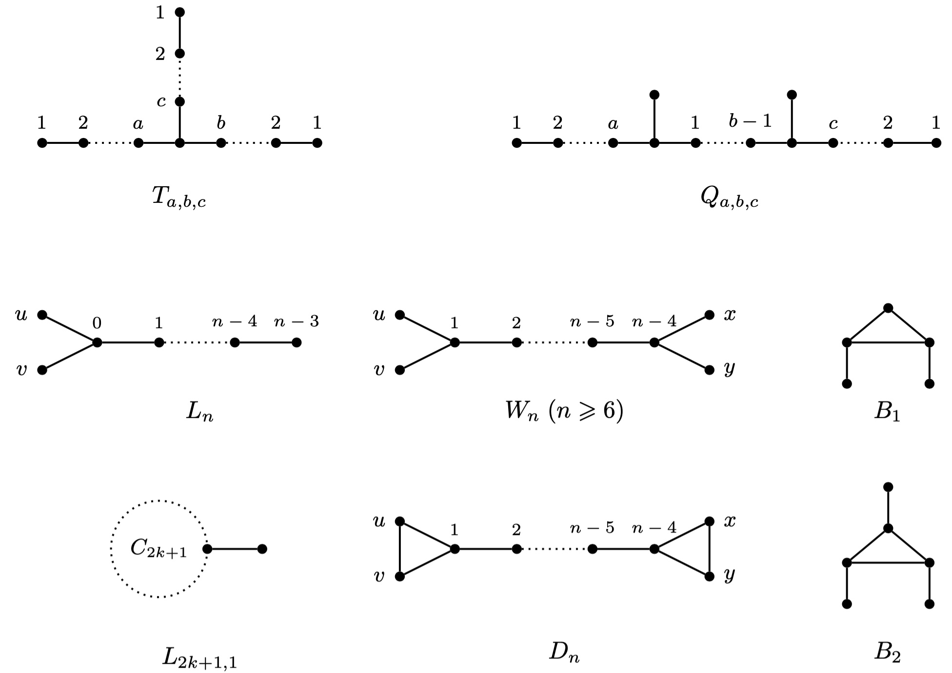
Figure 1. Some graphs used in the paper.

2. Adjacency matrix

The Hoffman program was initially carried out with respect to the adjacency matrix. Hoffman [21] contributed with the following pioneering result.

Theorem 2.1.

[21, Hoffman’s theorem] Let $\tau$ denote the number $(\sqrt{5}+1)/2$. For $n\in\mathbb{N}$, let $\eta_{n}=\beta_{n}^{\frac{1}{2}}+\beta_{n}^{-\frac{1}{2}}$, where $\beta_{n}$ is the positive root of

$$\phi_{n}(x)=x^{n+1}-(1+x+x^{2}+\cdots+x^{n-1}).$$

The numbers $2=\eta_{1}<\eta_{2}<\cdots$ are the only $A$-limit points of the $A$-spectral radius of graphs smaller than $\lim\limits_{n\rightarrow\infty}\eta_{n}=\tau^{\frac{1}{2}}+\tau^{-\frac{1}{2}}=\sqrt{2+\sqrt{5}}.$

As recalled in Section 1, the $A$-spectral radius of a graph $G$ is also the largest eigenvalue of $A(G)$. This is due to the fact that $A$ is non-negative (see [14, Theorem 0.2]).

Encouraged by Hoffman, Shearer [41] subsequently determined all the remaining $A$-limit points. In fact, he proved the following theorem.

Theorem 2.2.

[41] For any $\lambda\geq\sqrt{2+\sqrt{5}}=2.058+$, there exists a sequence of graphs $\{G_{k}\,|\,k\in\mathbb{N}\}$ such that $\lim\limits_{k\rightarrow\infty}\rho_{A}(G_{k})=\lambda$.

The graphs with $A$-index at most $\sqrt{2+\sqrt{5}}$ was characterized step-by-step in [42, 21, 15, 7]. More precisely, Smith [42] determined all the connected graphs whose $A$-index is not greater than 2. They are now known in the literature as Smith graphs. After [21], Cvetković et al. determined the structure of graphs with $A$-index between 2 and $\sqrt{2+\sqrt{5}}$ in [15]. Their description was completed a few years later by Brouwer and Neumaier [7]. We summarize such achievements in the following theorem.

Theorem 2.3.

Let $\rho_{1}=\sqrt{2+\sqrt{5}}$. The three sets $\mathcal{G}^{<2}_{A}$, $\mathcal{G}^{2}_{A}$ and $\mathcal{G}^{>2}_{A}\cap\mathcal{G}^{<\rho_{1}}_{A}$ can be described as follows.

• [42] $\mathcal{G}^{<2}_{A}=\{P_{n},\;T_{1,1,n},\;T_{1,2,c}\mid n\in\mathbb{N},\;2\leqslant c\leqslant 4\}$.
  

• [42] $\mathcal{G}^{2}_{A}=\{C_{n+2},\;W_{n+5}\mid n\in\mathbb{N}\}\cup\{K_{1,4},\;T_{2,2,2},\;T_{1,2,5},\;T_{1,3,3}\}$.
  

• [7, 15] $\mathcal{G}^{>2}_{A}\cap\mathcal{G}^{<\rho_{1}}_{A}$ is the disjoint union of the subsets

  $$\mathcal{T}_{1}=\{T_{1,2,n+5},\;T_{1,n+2,m+3},\;T_{2,2,n+2}\mid n\in\mathbb{N},\;m\geqslant n-1\}\cup\{T_{2,3,3}\}.$$

  and

  $${\mathcal{T}}_{2}=\{Q_{1,1,2},\;Q_{2,4,2},\;Q_{2,5,3},\;Q_{3,7,3},\;Q_{3,8,4}\}\cup\{Q_{a,b,c}\mid(a,c)\in\mathbb{N}^{2}\setminus(1,1),\;b\geqslant b^{*}(a,c)\},$$

  where $b^{*}(a,c)=\begin{cases}a+c+2,\qquad\text{ for $a>2$},\\ c+3,\qquad\quad\;\;\,\text{ for $a=2$},\\ c,\qquad\qquad\quad\;\,\text{ for $a=1$}.\\ \end{cases}$

Woo and Neumaier [54] characterized the structure of the graphs whose $A$-index is between $\sqrt{2+\sqrt{5}}$ and $\frac{3}{2}\sqrt{2}$. We recall that an open quipu is a tree of maximum vertex degree $3$ such that all vertices of degree 3 lie on a path; a closed quipu is a connected graph of maximum vertex degree $3$ containing just one cycle $C$, and all vertices of degree 3 lie on $C$; finally, a dagger is a path with a $3$-claw attached to an end vertex.

Theorem 2.4.

[54] Let $\rho_{1}=\sqrt{2+\sqrt{5}}$ and $\rho_{2}=\frac{3}{2}\sqrt{2}$. A graph in $\mathcal{G}^{>\rho_{1}}_{A}\cap\mathcal{G}^{<\rho_{2}}_{A}$ is either an open quipu, a closed quipu, or a dagger.

All daggers are in $\mathcal{G}^{<\rho_{2}}_{A}$. On the contrary, many open quipus and closed quipus have spectral radii greater than $\frac{3}{2}\sqrt{2}$, and the structural conditions ensuring whether a quipu $T$ is in $\mathcal{G}^{<\rho_{2}}_{A}$ or not are still to be completely determined. In any case, restrictions on the diameters of quipus belonging to $\mathcal{G}^{<\rho_{2}}_{A}$ are given by the following theorem.

Theorem 2.5.

[24] Let $\rho_{2}=\frac{3}{2}\sqrt{2}$. If an open quipu with $n\geqslant 6$ vertices belongs to $\mathcal{G}^{<\rho_{2}}_{A}$, then its diameter is at least $(2n-2)/3$. If a closed quipu with $n\geqslant 13$ vertices belongs to $\mathcal{G}^{<\rho_{2}}_{A}$, then its diameter lies in the interval $(n/3,(2n-2)/3]$.

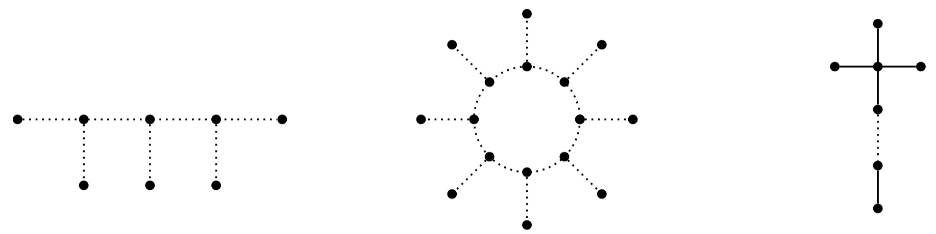
Figure 2. From left to right, an open quipu, a closed quipu and a dagger

3. Laplacian matrix

Guo obtained a Hoffman-like theorem for the $L$-spectrum in [17]. More precisely, he obtained the $L$-limit points of the $L$-spectral radius of graphs less than $2+\omega+\omega^{-1}=4.38+$, where $\omega=\frac{{\;}1{\;}}{3}\left((19+3\sqrt{33})^{\frac{{\;}1{\;}}{3}}+(19-3\sqrt{33})^{\frac{{\;}1{\;}}{3}}+1\right)$.

Theorem 3.1.

[17] Let $\beta_{0}=1$ and $\beta_{n}(n\geq 1)$ be the largest positive root of

$$f_{n}(x)=x^{n+1}-(1+x+\cdots+x^{n-1})(\sqrt{x}+1)^{2}.$$

Let $\alpha_{n}=2+\beta_{n}^{\frac{1}{2}}+\beta_{n}^{\frac{-1}{2}}$. Then,

$$4=\alpha_{0}<\alpha_{1}<\alpha_{2}<\cdots$$

are all the limit points of $L$-spectral radius of graphs less than $\lim\limits_{n\rightarrow\infty}\alpha_{n}=2+\omega+\omega^{-1}$.

Until now, the $L$-limit points of $L$-spectral radius of graphs no less than $2+\omega+\omega^{-1}$ have not been investigated. We here propose a conjecture. If true, it would be the Laplacian-counterpart of Shearer’s result on $A$-limit points.

Conjecture 1.

For any $\sigma\geq 2+\omega+\omega^{-1}$, there exists a sequence of graphs $\{G_{k}\,|\,k\in\mathbb{N}\}$ such that $\lim\limits_{k\rightarrow\infty}\rho_{L}(G_{k})=\sigma$.

Graphs with relatively small $L$-spectral radius were independently studied by several scholars. Omidi [36, 37] characterized the connected graphs whose $L$-index does not exceed $(5+\sqrt{13})/2$ (note that $2+\omega+\omega^{-1}=4.38+>(5+\sqrt{13})/2=4.302+$). Later on, Simić, Huang, Belardo and the first author of this paper [49] studied the spectral determination of disjoint union of graphs with $L$-index at most $4$. Wang, Belardo and Huang [46] also characterized the graphs whose $L$-index lies either in $[4,2+\sqrt{5}]$, $(2+\sqrt{5},2+\omega+\omega^{-1}]$ or $(2+\omega+\omega^{-1},4.5]$. Next theorem outlines in more details the results summarized in this paragraph. The last sentence in its statement depends on results concerning the $Q$-index recalled in Section 4 and proved in [46].

Theorem 3.2.

Let $\tau_{1}=2+\sqrt{5}$ and $\tau_{2}=2+\omega+\omega^{-1}$. The following equalities of sets hold.

• [36, 49] $\mathcal{G}^{<4}_{L}=\{P_{n},C_{2n+1}\mid n\in\mathbb{N}\}$.
  

• [36, 49] $\mathcal{G}^{4}_{L}=\{K_{1,3},K_{1,3}+e,K_{4}-e,K_{4}\}\cup\{C_{2k}\mid k\geq 2\}$.
  

• [46] $\mathcal{G}^{>4}_{L}\cap\mathcal{G}^{\leqslant\tau_{1}}_{L}=\{T_{1,1,n-3},\;L_{n}\mid n\geq 5\}$;
  

• [46] $\mathcal{G}^{>\tau_{1}}_{L}\cap\mathcal{G}^{\leqslant\tau_{2}}_{L}=\bigcup_{i=1}^{5}\mathcal{U}_{i}$, where

  $$\mathcal{U}_{1}=\{B_{1},B_{2}\};\qquad\mathcal{U}_{2}=\{L_{2k+2,1}\mid k\geq 2\};\qquad\mathcal{U}_{3}=\{T_{1,b,c}\mid c\geq b\geq 2\};$$

  $$\mathcal{U}_{4}=\{Q_{a,b,c}\mid b\geq a+c+1\};\qquad\mathcal{U}_{5}=\{W_{n},D_{n}-xy,D_{n}\mid n\geq 8\}.$$

Moreover, the set $\mathcal{G}^{>\tau_{2}}_{L}\cap\mathcal{G}^{\leqslant 4.5}_{L}$ just contains open and closed quipus.

4. Signless Laplacian matrix

Inspired by Hoffman’s theorem and Guo’s Theorem 3.1, the first authors of this paper et al.  [47] determined the $Q$-limit points smaller than $2+\varepsilon$, where $\varepsilon=\frac{{\;}1{\;}}{3}\left((54-6\sqrt{33})^{\frac{{\;}1{\;}}{3}}+(54+6\sqrt{33})^{\frac{{\;}1{\;}}{3}}\right)$. Note that $\varepsilon=\omega+\omega^{-1}=2.38+$, where $\omega$ is the number defined Section 3. The $L$-limit points and the $Q$-limits points less than $2+\varepsilon$ are the same. This is not surprising, since the proof of [47, Theorem 3.1] consists in a reduction to trees, and it is well-known the $L$- and $Q$-spectra of bipartite graphs are equal.

Theorem 4.1.

[47] Let $\beta_{0}=1$ and $\beta_{n}(n\geq 1)$ be the largest positive root of

$$f_{n}(x)=x^{n+1}-(1+x+\cdots+x^{n-1})(\sqrt{x}+1)^{2}.$$

Let $\alpha_{n}=2+\beta_{n}^{\frac{1}{2}}+\beta_{n}^{\frac{-1}{2}}$. Then

$$4=\alpha_{0}<\alpha_{1}<\alpha_{2}<\cdots$$

are all the limit points of the $L$-index and the $Q$-index of graphs less than $\lim\limits_{n\rightarrow\infty}\alpha_{n}=2+\varepsilon$, where $\varepsilon=\frac{{\;}1{\;}}{3}\left((54-6\sqrt{33})^{\frac{{\;}1{\;}}{3}}+(54+6\sqrt{33})^{\frac{{\;}1{\;}}{3}}\right)=2.38+$.

So far, the $Q$-limit points of the $Q$-index which are not less than $2+\varepsilon$ have not yet been identified. As for the correspondent problem in the $L$-context, we state the following conjecture.

Conjecture 2.

For any $\theta\geq 2+\varepsilon$, there exists a sequence of graphs $\{G_{k}\,|\,k\in\mathbb{N}\}$ such that $\lim\limits_{k\rightarrow\infty}\rho_{Q}(G_{k})=\theta$.

The graphs with $Q$-index not exceeding $2+\varepsilon$ were gradually characterized in [10, 48, 6]. More in details, Cvetković, Rowlinson and Simić [10] characterized the graphs in $\mathcal{G}^{\leqslant 4}_{Q}$. Afterwards, Wang et al. [48] started to describe the graphs in $\mathcal{G}^{>4}_{Q}\cap\mathcal{G}^{\leqslant 2+\sqrt{5}}_{Q}$ and in $\mathcal{G}^{>2+\sqrt{5}}_{Q}\cap\mathcal{G}^{\leqslant 2+\varepsilon}_{Q}$ Their work was brought to completion two years later by Belardo et al. in [6]. Finally, Wang et al. [48] gave the structure of graphs in $\mathcal{G}^{>2+\varepsilon}_{Q}\cap\mathcal{G}^{\leqslant 4.5}_{Q}$.

Theorem 4.2.

Let $\tau_{1}=2+\sqrt{5}$ and $\tau_{2}=2+\varepsilon$. The following equalities of sets hold.

• [10] $\mathcal{G}^{<4}_{Q}=\{P_{n}\mid n\in\mathbb{N}\}$.
  

• [10] $\mathcal{G}^{4}_{Q}=\{K_{1,3},C_{n}\mid n\geqslant 3\}$;
  

• [48] $\mathcal{G}^{>4}_{Q}\cap\mathcal{G}^{\leqslant\tau_{1}}_{Q}=\{T_{1,1,n-3}\mid n\geq 5\}$;
  

• [48, 6] $\mathcal{G}^{>\tau_{1}}_{Q}\cap\mathcal{G}^{\leqslant\tau_{2}}_{Q}=\{T_{1,b,c}\mid c\geq b\geq 2\}\cup\{Q_{a,b,c}\mid b\geq a+c+1\}$.

Moreover, the set $\mathcal{G}^{>\tau_{2}}_{Q}\cap\mathcal{G}^{\leqslant 4.5}_{Q}$ just contains open and closed quipus.

5. Hermitian adjacency matrix

Liu and Li [30] and Guo and Mohar [18] independently introduced the Hermitian adjacency matrix $\mathcal{H}(G)$ associated to a mixed graph $G$.

We recall that a mixed graph $G$ consists of a vertex set $V=V(G)$ and an arc set

$$\vv{E}(G)\subseteq(V\times V)\setminus\{(v,v)\mid v\in V\}.$$

Note that if an arc $uv=(u,v)$ belongs to $\vv{E}(G)$, then the arc $vu$ may or may not belong to $\vv{E}(G)$. A digon $\{u,v\}$ is determined by every pair of arcs $uv$ and $vu$ both belonging to $\vv{E}(G)$, and can be regarded as an undirected edge connecting $u$ and $v$. Mixed graphs are also called directed graphs or digraphs in [19]. The underlying graph of a digraph $G$ is the graph with vertex-set $V$ and edge-set $E=\{\{x,y\}\mid xy\in\vv{E}(G)\;\text{or}\;yx\in\vv{E}(G)\}$.

The entries $\mathcal{H}_{uv}$ of the Hermitian adjacency matrix $\mathcal{H}(G)\in\mathbb{C}^{|V|\times|V|}$ are as follows:

$$\mathcal{H}_{uv}=\begin{cases}\phantom{-}1\quad\text{if $uv$ and $vu\in\vv{E}(G)$};\\ \phantom{-}i\quad\text{if $uv\in\vv{E}(G)$ and $vu\not\in\vv{E}(G)$};\\ -i\quad\text{if $uv\not\in\vv{E}(G)$ and $vu\in\vv{E}(G)$};\\ \phantom{-}0\quad\text{otherwise}.\end{cases}$$

Spectral properties of the $\mathcal{H}$-matrix have been investigated in [11, 12, 16, 19, 20, 27, 45, 51, 52, 53]. Let $uv$ an arc in $\vv{E}(G)$ such that $vu\not\in\vv{E}(G)$. ‘Reversing the direction (or the orientation) of an arc $uv$’ means to consider the mixed graph $G^{\prime}$ obtained from $G$ by replacing $uv$ with $vu$ in its arc set. The $\mathcal{H}$-spectrum is preserved if we reverse the direction of all arcs not involved in a digon. The mixed graph obtained in this way is called the converse of the original one. However, Guo and Mohar [18, 27] unveiled a more complicated transformation leaving the $\mathcal{H}$-spectrum unchanged. Suppose that the vertex-set of $G$ is partitioned in four (possibly empty) sets, $V(G)=V_{1}\cup V_{-1}\cup V_{i}\cup V_{-i}$. An arc $xy\in\vv{E}(G)$ is said to be of type $(j,k)$ for $j,k\in\{\pm 1,\pm i\}$ if $x\in V_{j}$ and $y\in V_{k}$. The partition is admissible if the following conditions hold:

• There are no digons of types $(1,-1)$ or $(i,-i)$.
  

• All edges of types $(1,i)$, $(i,-1)$, $(-1,-i)$, $(-i,1)$ are contained in digons.
  

A four-way switching with respect to a partition $V(G)=V_{1}\cup V_{-1}\cup V_{i}\cup V_{-i}$ is the operation of changing $G$ into the mixed graph $G^{\prime}$ by making the following changes:

• reversing the direction of all arcs of types $(1,-1),(-1,1),(i,-i),(-i,i)$;
  

• (replacing each digon of type $(1,i)$ with a single arc directed from $V_{1}$ to $V_{i}$ and replacing each digon of type $(-1,-i)$ with a single arc directed from $V_{-1}$ to $V_{-i}$;
  

• replacing each digon of type $(1,-i)$ with a single arc directed from $V_{-i}$ to $V_{1}$ and replacing each digon of type $(-1,i)$ with a single arc directed from $V_{i}$ to $V_{-1}$;
  

• replacing each non-digon of type $(1,-i),(-1,i),(i,1)$ or $(-i,-1)$ with the digon.
  

Two mixed graphs $G_{1}$ and $G_{2}$ are switching equivalent if, after choosing an admissible partition on their common vertex set, one of them can be obtained from the other by a suitable sequence of four-way switchings and the operation of taking the converse. It turns out that two switching equivalent mixed graphs have the same $\mathcal{H}$-spectrum. Guo and Mohar [19] make use of switching equivalence to list all connected digraphs with $\mathcal{H}$-index less than 2.

Let $F$ be any forest. We regard $F$ as the mixed graph obtained by replacing each of its edges by a digon. From this perspective $\mathcal{H}(F)=A(F)$, and $\rho_{\mathcal{H}}(T)=\rho_{A}(T)$ for any tree $T$. All mixed graphs whose underlying graph is a forest $F$ are switching equivalent [18, 30]; therefore, their $\mathcal{H}$-spectra are all equal to the $A$-spectrum of $F$.

To describe Guo and Mohar’s results, we still need some extra notation. We denote by $D_{n}$ the directed cycle on $n$ vertices. The digraph $\widetilde{C_{n}}$ is obtained from $D_{n}$ by reversing the direction of one of the directed edges. The digraph $\widetilde{C_{n}^{\prime}}$ is the digraph obtained from $D_{n}$ by replacing one edge with a digon. The digraph $\widetilde{C_{n}^{\prime\prime}}$ is the digraph obtained from $D_{n}$ by taking two consecutive arcs and then replacing the first one by a digon and reversing the direction of the second one. A quadrangle is a mixed graph whose underlying graph is $C_{4}$. A quadrangle is positive if either of the following holds: it has four digons, or it has two digons and the two non-digon arcs are oriented differently with respect to the order on the cycle $C_{4}$ (one clockwise and one anticlockwise), or it has no digons and two pairs of oppositely oriented arcs, or it has no digons and all arcs are oriented in the same direction with respect to the order on the cycle. It is a negative quadrangle if it has an even number of digons and does not fall into the three cases of positive quadrangles.

Let $a,b,c,d$ be nonnegative integers. Let $\Box_{abcd}$ be a digraph obtained from a negative quadrangle with (consecutive) vertices $v_{1},v_{2},v_{3},v_{4}$ by adding directed paths of lengths $a,b,c,d$ that are attached to $v_{1},v_{2},v_{3},v_{4}$ respectively. For the mixed graphs in the statement of Theorem 5.1 and not defined above, see Fig. 3, where each arrow from a vertex $u$ to $v$ in $V(G)$ means that the arc $uv$ belong to $\vv{E}(G)$.

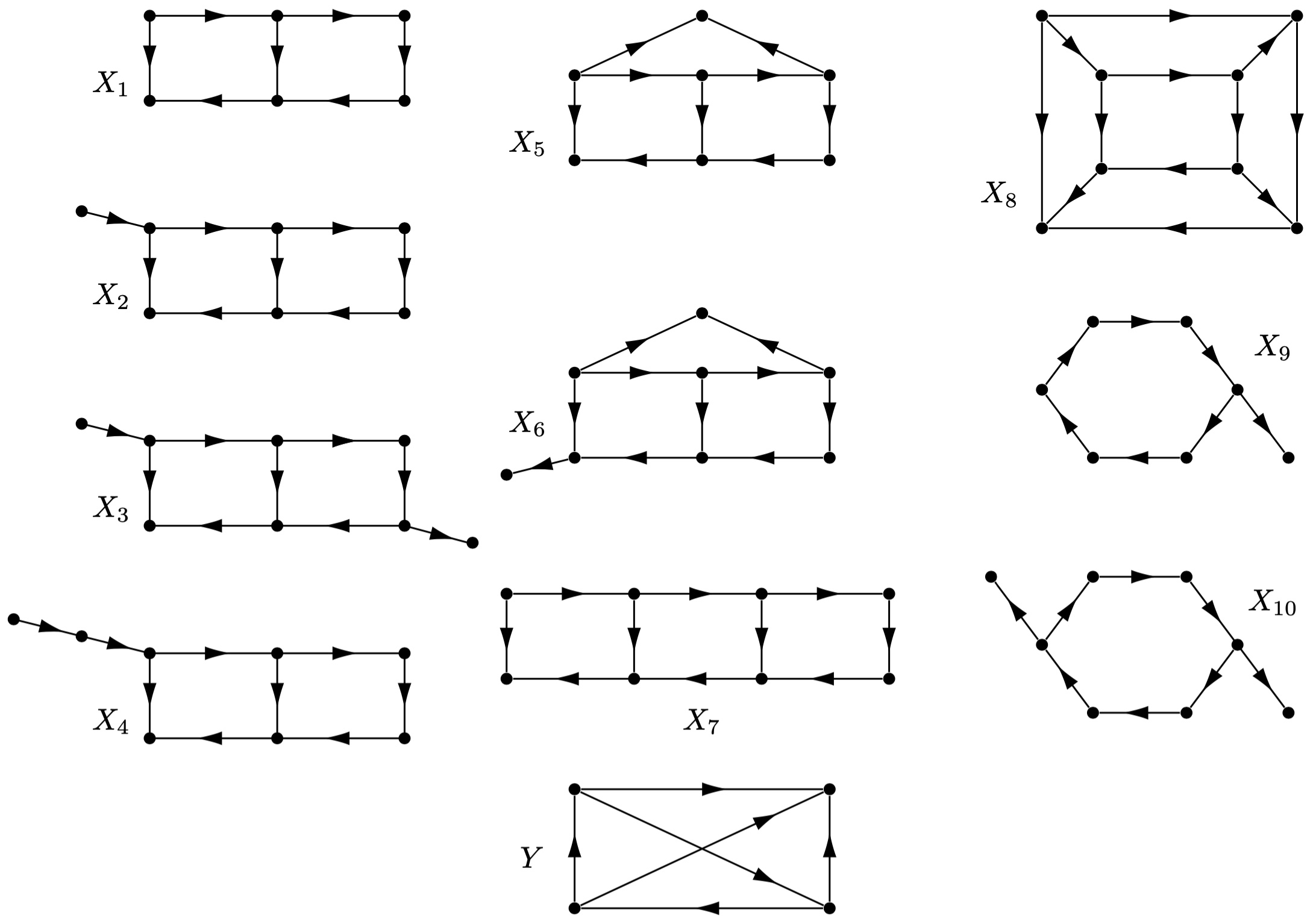
Figure 3. The mixed graphs $X_{i}$ for $1\leqslant i\leqslant 10$ and $Y$.

Theorem 5.1.

[19] A connected digraph $G$ has $\rho_{\mathcal{H}}(G)<2$ if and only if $G$ is switching equivalent to one of the following:

• $P_{n}$;
  

• $D_{n}$ for $n\not\equiv 0\mod 4$;
  

• $\widetilde{C_{n}}$ for $n\not\equiv 2\mod 4$;
  

• $\widetilde{C_{n}^{\prime}}$ $n\not\equiv 3\mod 4$;
  

• $\widetilde{C_{n}^{\prime\prime}}$ $n\not\equiv 1\mod 4$;
  

• $T_{a,1,1}$, with $a\in\mathbb{N}$;
  

• $T_{a,2,1}$, with $2\leqslant a\leqslant 4$;
  

• $X_{i}$ for $1\leqslant i\leqslant 10$;
  

• $Y$;
  

• $\square_{a,0,c,0}$, where $a\geq c\geq 0$;
  

• $\square_{3,1,0,0},\square_{2,1,1,0},\square_{2,1,0,0},$
  $\square_{1,1,1,1},\square_{1,1,1,0},\square_{1,1,0,0}$;
  

• the digraph obtained from the directed triangle $D_{3}$ by adding a vertex and an arc from this vertex to one of the vertices of $D_{3}$;
  

The following corollary follows from the above theorem.

Corollary 5.2.

The smallest limit point for the $\mathcal{H}$-spectral radius of mixed graphs is $2$.

As in previous sections, let $\rho_{1}=\sqrt{2+\sqrt{5}}$. By Theorem 2.3 we see that there exist infinite families of trees (and hence of mixed graphs) in ${\mathcal{G}}_{A}^{2}$ and in ${\mathcal{G}}_{A}^{>2}\cap{\mathcal{G}}_{A}^{<\rho_{1}}$. Thereby, it makes sense to consider the following problem.

Problem 1.

For the Hoffman program of mixed graphs with respect to the $\mathcal{H}$-matrix,

• determine all the $\mathcal{H}$-limit points of the $\mathcal{H}$-spectral radius of mixed graphs less than $\sqrt{2+\sqrt{5}}$;

• characterize the graphs with $\rho_{\mathcal{H}}(G)=2$ and $\rho_{\mathcal{H}}(G)\in(2,\sqrt{2+\sqrt{5}}]$.

6. Signed-adjacency matrix

A signed graph $\Gamma=(G;\sigma)$ is a non-empty graph $G=(V,E)$, with vertex set $V$ and edge set $E$, together with a function $\sigma:E\rightarrow\{+1,-1\}$ assigning a positive or negative sign to each edge. The (unsigned) graph $G$ is said to be the underlying graph of $\Gamma$, and the function $\sigma$ is called the signature of $\Gamma$. Unsigned graphs are treated as signed graphs equipped with the all-positive signature $\sigma^{+}$ such that $\sigma^{+}(E)=\{1\}$. Clearly, the all-negative signature $\sigma^{-}=-\sigma^{+}$ maps all edges onto $-1$.

For a subset $U\subseteq V(G)$, let $\Gamma^{U}$ be the signed graph obtained from $\Gamma$ by reversing the signs of the edges in the cut $[U,V(G)\backslash U]$, namely $\sigma_{\Gamma^{U}}(e)=-\sigma_{\Gamma}(e)$ for any edge $e$ between $U$ and $VG)\backslash U$, and $\sigma_{\Gamma^{U}}(e)=\sigma_{\Gamma}(e)$ otherwise. The signed graph $\Gamma$ and $\Gamma^{U}$ (and the signatures $\sigma_{\Gamma}$ and $\sigma_{\Gamma^{U}}$ as well) are said to be switching equivalent.

The signed adjacency matrix $\mathcal{S}(\Gamma)=(s_{ij})$ is the symmetric of $\{0,1,-1\}$-matrix such that $s_{ij}=\sigma(ij)$ whenever the vertices $i$ and $j$ are adjacent, and $a_{ij}=0$ otherwise. The above switching can also be explained from a matrix viewpoint. In fact, let $\Gamma$ and $\Gamma^{U}$ be two switching equivalent graphs. Consider the signature matrix $S_{U}={\rm diag}(\epsilon_{1},\epsilon_{2},\cdots,\epsilon_{n})$ such that

$$\epsilon_{i}=\begin{cases}+1&\text{if $i\in U$};\\ -1,&\text{if $i\in\Gamma\backslash U$}.\end{cases}$$

It is easy to check that $A(\Gamma^{U})=S_{U}A(\Gamma)S_{U}$. In other words, signed graphs from the same switching class share similar graph matrices by means of signature matrices. This in particular implies that $\Gamma$ and $\Gamma^{U}$ are $\mathcal{S}$-cospectral. It is worthy to note that all signatures on forests are switching equivalent; moreover, the $\mathcal{S}$-spectral radius is not always equal to the largest $\mathcal{S}$-eigenvalue, the minimal example being $(C_{3},\sigma^{-})$ whose $\mathcal{S}$-spectrum is $\{-2,1,1\}$.

For basic results in the theory of signed graphs, the reader is referred to [59, 60]. On the same topic, Zaslavsky currently edits two dynamic surveys [57, 58]. For a recent list of open problems concerning signed graphs, see [5].

We now focus on Hoffman program in relation to signed graphs.

Proposition 6.1.

The smallest limit point of $\mathcal{S}$-spectral radius of signed graphs is $2$.

Proof.

The real number $2$ is surely an ${\mathcal{S}}$-limit point. In fact $\lim_{k\rightarrow\infty}\rho_{\mathcal{S}}(P_{k})=2$. In order to prove that there are no ${\mathcal{S}}$-limit points less than $2$, let $\{\Gamma_{k}=(G_{k},\sigma_{k})\,|\,k\in\mathbb{N}\}$ be a sequence of signed graphs such that

$$\rho_{\mathcal{S}}(\Gamma_{i})\neq\rho_{\mathcal{S}}(\Gamma_{j})\quad\text{whenever $i\neq j$},\quad\text{and}\quad\lim_{k\rightarrow\infty}\rho_{\mathcal{S}}(\Gamma_{k})=\gamma\leqslant 2.$$

Since the $\Gamma_{i}$’s are pairwise distinct, and their maximum vertex degree is bounded being $\sqrt{\Delta(G_{i})}\leqslant\rho_{\mathcal{S}}(\Gamma_{i})$, then $\lim_{k\rightarrow\infty}\mathrm{diam}(\Gamma_{k})=+\infty$. It follows that there exists a subsequence of signed graphs $\{\Gamma_{k_{n}}\,|\,n\in\mathbb{N}\}$ such that $(P_{n},\sigma_{|P_{n}})$ is a subgraph of $\Gamma_{k_{n}}$. Now, $(P_{n},(\sigma_{k_{n}})_{|P_{n}})$ and $P_{n}$ are switching equivalent, and, as a consequence of Cauchy Interlacing Theorem holding for all Hermitian matrices (see, for instance [14, Theorem 0.10]), we have $\rho_{\mathcal{S}}(P_{n},(\sigma_{k_{n}})_{|P_{n}})\leqslant\rho_{\mathcal{S}}(\Gamma_{k_{n}})$. Hence,

$$2=\lim_{n\rightarrow\infty}\rho_{A}(P_{n})=\lim_{n\rightarrow\infty}\rho_{\mathcal{S}}(P_{n},(\sigma_{k_{n}})_{|P_{n}})\leq\lim_{k\rightarrow\infty}\rho_{\mathcal{S}}(\Gamma_{k})=\gamma\leq 2,$$

which is possible only if $\gamma=2$. ∎

A (signed) graph is said to be maximal with respect to some property $\mathcal{P}$ if it is not a proper induced subgraph of some other (signed) graph satisfying $\mathcal{P}$. All maximal signed graphs in $\mathcal{G}_{\mathcal{S}}^{\leqslant 2}$ have been detected by McKee and Smyth [32]; they are the signed graphs $T_{2k}$ ($k\geqslant 3$), $S_{14}$ and $S_{16}$ depicted in Fig. 4.

Theorem 6.2.

[32] Signed graphs in $\mathcal{G}_{\mathcal{S}}^{\leqslant 2}$ are switching equivalent to the induced subgraphs of (i) the $2k$-vertex toral tessellation $T_{2k}$, for $k\geqslant 3$; (ii) the $14$-vertex signed graph $S_{14}$; (iii) the $16$-vertex signed hypercube $S_{16}$. Moreover, $\rho_{\mathcal{S}}(S_{14})=\rho_{\mathcal{S}}(S_{16})=\rho_{\mathcal{S}}(T_{2k})=2$ for all $k\geqslant 3$.

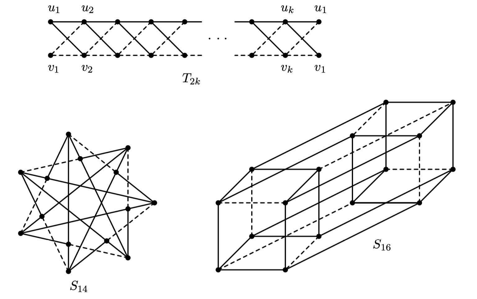
Figure 4. Maximal signed graphs in $\mathcal{G}_{\mathcal{S}}^{\leqslant 2}$. Negative edges are depicted by dashed lines.

As proved, for instance, in [5, Theorem 2.5], for a signed graph $\Gamma=(G;\sigma)$ we obtain $\rho_{\mathcal{S}}(\Gamma)\leq\rho_{A}(G)$. Thus, the $A$-spectral radius of the underlying graph naturally limits the magnitude of the eigenvalues of the corresponding signed graph.

Problem 2.

[5, Problem 3.11] Let $\rho_{1}=\sqrt{2+\sqrt{5}}$. Characterize all signed graphs in $\mathcal{G}_{\mathcal{S}}^{\leqslant\rho_{1}}$.

Fortunately, the theory of limit points for the $\mathcal{S}$-spectral radius of signed graphs partially overlaps the one related to the $A$-index of unsigned graphs. For instance, since all signed graphs sharing a fixed forest $F$ as underlying graph are $\mathcal{S}$-cospectral, then $\rho_{\mathcal{S}}(F,\sigma)=\rho_{\mathcal{S}}(F,\sigma^{+})=\rho_{A}(F)$. It follows by Cauchy’s Interlacing Theorem that an acyclic subgraph of a graph in $\mathcal{G}_{\mathcal{S}}^{\leqslant\rho_{1}}$ necessarily appears among the ones listed in Theorem 2.3.

For the same reason, we can use the very same sequences of (acyclic) open caterpillars used by Shearer in its proof of Theorem 2.2, to prove the following proposition concerning $\mathcal{S}$-spectra (an open caterpillar is a graph such that the removal of all pendant vertices results in a chordless path).

Proposition 6.3.

For any $\lambda\geq\sqrt{2+\sqrt{5}}$, there exists a sequence of signed caterpillars $\{\Gamma_{k}\,|\,k\in\mathbb{N}\}$ such that $\lim\limits_{k\rightarrow\infty}\rho_{\mathcal{S}}(\Gamma_{k})=\lambda$.

Although Hoffman’s theorem was ultimately based on a tree, its proof cannot be directly translated to $\mathcal{S}$-spectra. In fact, if $G$ is not a tree or a cycle, then $\rho_{A}(G)>(\sqrt{5}+1)/2$, whereas $\mathcal{G}_{\mathcal{S}}^{<2}$ contains signed unicyclic graphs which are not cycles and signed bicyclic graphs as well (see [2, 4].

Problem 3.

Characterize the limit points of the $\mathcal{S}$-spectral radius of signed graphs less than $\sqrt{2+\sqrt{5}}$.

7. Skew-adjacency matrix

To our knowledge, the first attempts to build a spectral theory based on skew-adjacency matrices associated to oriented graphs go back to around 2009 [1, 23, 40]. The paper [8] by Cavers, Cioabă et al. provides a comprehensive introduction to this topic. An oriented graph is a mixed graph without digons. In any case, our notation and terminology will be largely consistent with [43].

Let $G=(V,E)$ be an undirected non-empty graph of order $n$, an oriented graph is a pair $\widetilde{G}=(G,\tilde{\sigma})$, where the edge orientation $\tilde{\sigma}:E\rightarrow V$ is a map satisfying $\tilde{\sigma}(ij)\in\{i,j\}$, for every $ij\in E$. As in the context of signed graphs, we say that $G$ is the underlying graph of $\widetilde{G}$. The skew-adjacency matrix $S(\widetilde{G})=(\tilde{s}_{ij})$ of $\widetilde{G}$ is the $n\times n$ matrix defined by

$$\tilde{s}_{ij}=\begin{cases}\phantom{-}0&\text{if $ij\not\in E$};\\ \phantom{-}1&\text{if $\sigma^{\prime}(ij)=i$};\\ -1&\text{if $\sigma^{\prime}(ij)=j$}.\end{cases}$$

Note that the non-zero eigenvalues in ${\rm Sp}_{S}(\widetilde{G})$ are all purely imaginary, the matrix $S(\widetilde{G})$ being real skew symmetric. Then $S$-index $\rho_{S}(G^{\prime})$ of $G^{\prime}$ is defined as the largest modulus of the $S$-eigenvalues of $G^{\prime}$.

As in [43, 55, 56], if $\sigma(ij)=j$, we say that the edge $ij$ is oriented from $i$ to $j$ and write $i\!\rightarrow\!j$. Other authors adopt the other possible choice (see for instance, [8]); in any case, these two approaches are equivalent from a spectral perspective.

Clearly, the $S$-spectral radius $\rho_{S}(\widetilde{G})$ of $\widetilde{G}$ is given by the largest modulus of its $S$-eigenvalues. For any $U\subseteq V(G)$, let $\widetilde{G}^{U}$ be the oriented graph obtained from $\widetilde{G}$ by reversing the orientation of each edge between a vertex in $U$ and a vertex in $V(G)\backslash U$. We say that $\widetilde{G}$ and $\widetilde{G}^{U}$ are switching equivalent. Note that ${\rm Sp}_{S}(\widetilde{G}^{U})={\rm Sp}_{S}(\widetilde{G})$; in fact, $S(\widetilde{G}^{U})$ and $S(\widetilde{G}^{U})$ are similar via the matrix $S_{U}$ defined in Section 6.

Let $\widetilde{G}$ be an oriented graph with vertex set $\{u_{1},u_{2},\dots,u_{n}\}$. Stanić [43] defined the bipartite double ${\rm bd}(\widetilde{G})$ of $\widetilde{G}$ to be an oriented graph with vertices $\{u_{1}1,u_{1}2,u_{2}1,u_{2}2,\dots,u_{n}1,u_{n}2\}$ and $u_{i}k\rightarrow u_{j}l$ if and only if $u_{i}\rightarrow u_{j}$ and $k\neq l$. It is easily seen that $S({\rm bd}(G^{\prime}))$ is the Kronecker product $S(G^{\prime})\otimes A(K_{2})$.

We say that an oriented graph $\widetilde{G}=(G,\tilde{\sigma})$ is bipartite if so is $G$. The bipartite double ${\rm bd}(\widetilde{G})$ is bipartite and turns out to be connected if and only if $G$ is non-bipartite. Recall that, if $G$ is bipartite, then ${\rm Sp}_{A}(G)$ and ${\rm Sp}_{\mathcal{S}}(G,\sigma)$ are symmetric with respect to $0$ for each signature $\sigma$. Shader and So [40] proved that $G$ is bipartite if and only if there is an orientation $\tilde{\sigma}$ such that ${\rm Sp}_{S}(G,\tilde{\sigma})=i{\rm Sp}_{A}(G)$.

The problem of determining the oriented graphs in $\mathcal{G}_{S}^{\leqslant 2}$ has been first investigated by Xu and Gong, and some partial results are given in [55, 56]. Stanić [43] succeeded in detecting all maximal oriented graphs in $\mathcal{G}_{S}^{\leqslant 2}$ by forging a nice bridge between the $S$-eigenvalues of oriented graphs and the $\mathcal{S}$-spectrum of suitably associated signed graphs. Let $G=(V,E)$ be a non empty graph. A signature $\sigma:E\rightarrow\{-1,1\}$ is said to be associated to an edge orientation $\tilde{\sigma}:V\rightarrow E$ if

(1) $$\sigma(ik)\sigma(jk)=\tilde{s}_{ik}\tilde{s}_{jk}\;\text{holds for every pair of adjacent edges}\;ik\;\text{and}\;jk.$$

Together with the bipartite double Stanić provided the following two theorems (in their statements the exponential notation is used to denote the multiplicity of an eigenvalue).

Theorem 7.1.

[44] Let $\widetilde{G}=(G,\tilde{\sigma})$ be a bipartite oriented graph. If ${\rm rank}(S(\widetilde{G}))=2k$ and $\sigma$ is associated with $\tilde{\sigma}$, then

Theorem 7.2.

[44] Let $\widetilde{H}=(H,\tilde{\sigma})$ denote the bipartite double of the oriented graph $\widetilde{G}$, and let $\sigma$ be the signature on $H$ associated with $\tilde{\sigma}$. If ${\rm rank}(S(\widetilde{G}))=2k$, then

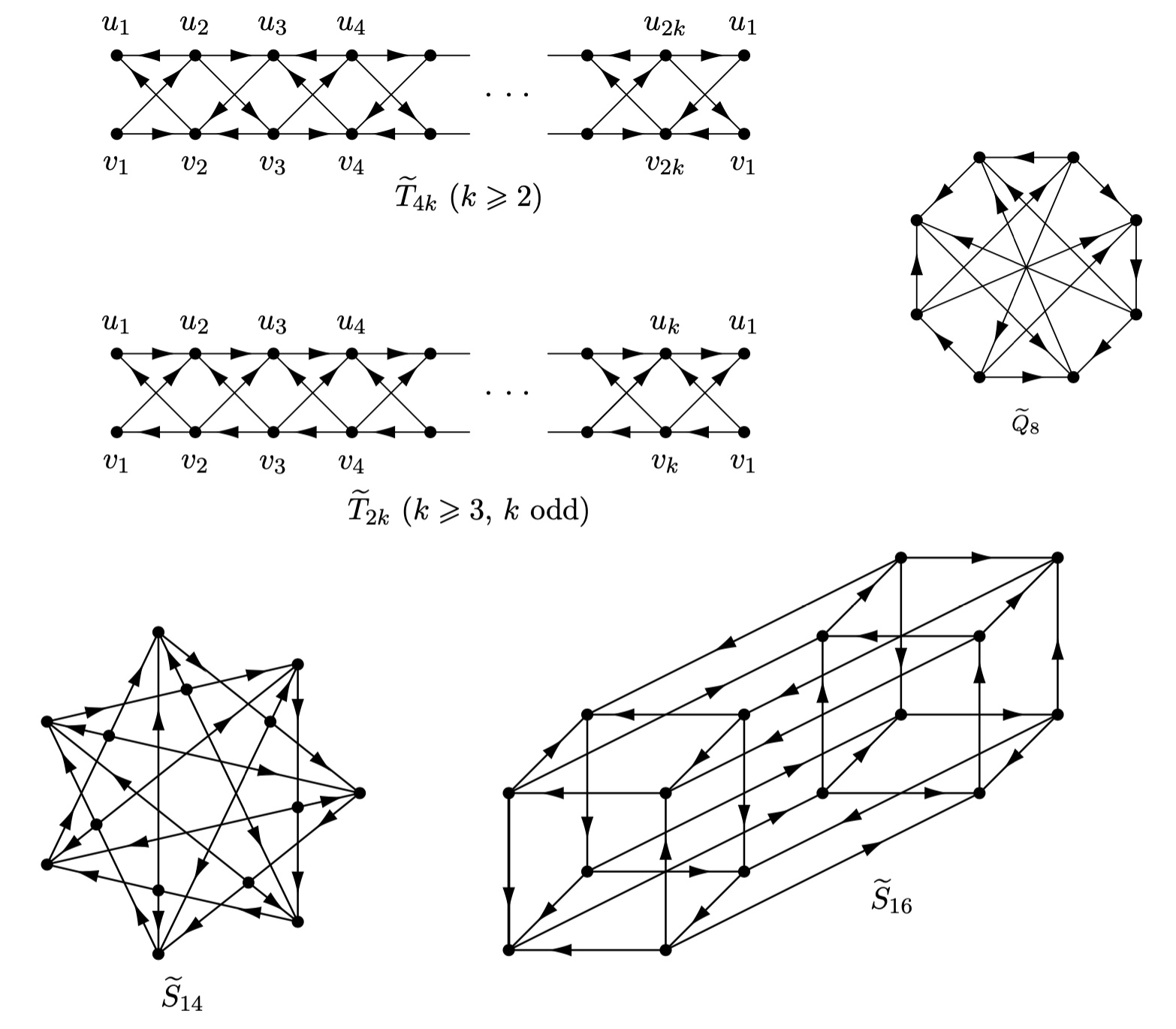
Figure 5. Maximal connected oriented graphs whose skew spectral radius does not exceed $2$.

Theorems 7.1 and 7.2, together with Theorem 6.2 and (1) are the key ingredients to show that if $\widetilde{G}$ is maximal and bipartite in ${\mathcal{G}}_{S}^{\leqslant 2}$, than it is switching equivalent to an object in the set $\mathcal{B}=\{\widetilde{S}_{14},\,\widetilde{Q}_{16},\,\widetilde{T}_{4k}\mid k\geqslant 2\}$ (see Fig. 5). Moreover, Stanić proved that if $\widetilde{G}$ is a connected oriented graph such that ${\rm bd}(\widetilde{G})\in\mathcal{B}$, then $\widetilde{G}$ is switching equivalent to either $\widetilde{Q}_{8}$ or $\widetilde{T}_{2k}$ with $k$ odd and $k\geqslant 3$. In particular, ${\rm bd}(\widetilde{Q}_{8})=\widetilde{Q}_{16}$, and, for any odd $k\geqslant 3$, ${\rm bd}(\widetilde{T}_{2k})=\widetilde{T}_{4k}$. Stanić’s results are summarized in the following theorem.

Theorem 7.3.

[43] Every maximal connected oriented graph whose skew spectral radius does not exceed $2$ is switching equivalent to one of following oriented graphs:

$$\widetilde{Q}_{8};\qquad\widetilde{S}_{14};\qquad\widetilde{Q}_{16};\qquad\widetilde{T}_{4h+2};\qquad\widetilde{T}_{4(h+1)}\quad(h\in\mathbb{N}).$$

They are all illustrated in Fig. 5.

Proposition 7.4.

For any $\lambda\geq\sqrt{2+\sqrt{5}}$, there exists a sequence of oriented graphs (namely, oriented caterpillars) $\{\widetilde{T}_{k}\,|\,k\in\mathbb{N}\}$ such that $\lim\limits_{k\rightarrow\infty}\rho_{S}(\widetilde{T}_{k})=\lambda$.

Proof.

In order to prove Theorem 2.2, for any $\lambda\geq\sqrt{2+\sqrt{5}}$ Shearer found a sequence of nested caterpillars $\{T_{k}\,|\,k\in\mathbb{N}\}$ such that $\lim\limits_{k\rightarrow\infty}\rho_{A}(T_{k})=\lambda$, In addition, Shader and So [40] showed that ${\rm Sp}_{S}(G,\tilde{\sigma})=i{\rm Sp}_{A}(G)$ for any orientation $\tilde{\sigma}$ if and only if $G$ is a forest. Thereby, for any oriented tree $(T,\tilde{\sigma})$, we have $\rho_{S}(T,\tilde{\sigma})=\rho_{A}(T)$. Thus, whatever orientation $\tilde{\sigma}_{k}$ we choose on the caterpillar $T_{k}$, we obtain $\rho_{S}(T_{i},\tilde{\sigma}_{i})\not=\rho_{S}(T_{j},\tilde{\sigma}_{j})$ whenever $i\not=j$ and $\lim\limits_{k\rightarrow\infty}\rho_{S}(T^{\prime}_{k})=\lambda$. ∎

8. Adjacency tensor

Since Lim [25] and Qi [38] independently introduced the eigenvalues of tensors or hypermatrices in 2005, the spectral theory of tensors has rapidly developed. A hypergraph $H$ is a pair $(V,E)$, where $E\subseteq\mathcal{P}(V)$. The elements of $V=V(H)$ are referred to as vertices and the elements of $E=E(H)$ are called edges. A hypergraph H is said to be k-uniform for an integer $k\geq 2$ if, for all $e\in E(H)$, $\left|e\right|=k$. To avoid trivial cases, we assume that $E$ is non-empty.

Definition 8.1.

[13] Let $H$ be an $r$-uniform hypergraph. Then the adjacency tensor of $H$ is defined as $\mathcal{A}(H)=(a_{{i_{1}}{i_{2}}\ldots{i_{r}}})$ $k$th order and $n$-dimensional tensor, where

$$a_{{i_{1}}{i_{2}}\ldots{i_{r}}}=\left\{\begin{array}[]{ll}\frac{1}{(r-1)!}&\mbox{if $\{i_{1},i_{2},\ldots,i_{r}\}\in E(H)$;}\\ 0&\mbox{otherwise}.\end{array}\right.$$

It is immediately seen that the adjacency tensor of hypergraphs is symmetric and generalizes the adjacency matrix of graphs. Let $[n]$ denote the set $\{1,2,\dots,n\}$. The polynomial form $f_{H}(x)$: $\mathbb{R}^{n}\rightarrow\mathbb{R}$ is defined for any vector ${\rm x}=(x_{1},\ldots,x_{n})\in\mathbb{R}^{n}$ as

(2) $$f_{H}(x)=\sum_{(i_{1},i_{2},\dots,i_{r})\in[n]^{r}}x_{i_{1}}x_{i_{2}}\cdots x_{i_{r}}=r\sum_{\{i_{1},i_{2},\ldots,i_{r}\}\in E(H)}x_{i_{1}}x_{i_{2}}\cdots x_{i_{r}}$$

Cooper and Dutle [13] call $\lambda\in\mathbb{C}$ an $H$-eigenvalue if there is a non-zero vector $x\in\mathbb{C}^{n}$ satisfying

$$\sum_{(i_{2},\dots,i_{r})\in[n]^{r-1}}a_{j,i_{2}\dots i_{r}}x_{i_{2}}\cdots x_{i_{r}}=\lambda x_{j}^{r-1}$$

for all $j\in[n]$, and prove that the $\mathcal{A}$-spectral radius of $H$, i.e.  the largest modulus among the $H$-eigenvalues, is also equal to

(3) $$\rho_{\mathcal{A}}(H)=\max_{\parallel{\rm x}\parallel_{r}=1}f_{H}(x),$$

the maximum value assumed by (2) over the $r$-norm unit sphere. Note that some authors (e.g. [31]) just skip the definition of an $H$-eigenvalue and define the $\mathcal{A}$-spectral radius of $H$ to be the real number (3). For more details on the eigenvalues of tensors see [25, 38].

Lu and Man [31] obtained the smallest limit point of $\mathcal{A}$-spectral radii of connected $r$-uniform hypergraphs. In fact, they proved the following result.

Theorem 8.1.

[31] The smallest limit point of $\mathcal{A}$-spectral radii of connected $r$-uniform hypergraphs is $\sqrt[r]{4}$.

For any real number $\rho$, we denote by $\mathcal{G}_{\mathcal{A}}^{\rho}$ (resp., $\mathcal{G}_{\mathcal{A}}^{<\rho}$) the set of uniform hypergraphs whose $\mathcal{A}$-spectral radius is equal to $\rho$ (resp. less than $\rho$). We also set $\rho_{r}=\sqrt[r]{4}$.

There is a rationale for the way many elements detected in $\mathcal{G}_{\mathcal{A}}^{<\rho}$ and in $\mathcal{G}_{\mathcal{A}}^{\rho}$ are denoted in [31] and below: they are the $r$-uniform counterpart of the Smith graphs listed in Theorem (i) and (ii); and the Smith graphs, in turn, are all simply-laced Dynkin diagrams. In $\mathcal{G}_{A}^{<2}$ we find, in fact, $P_{n}$, $T_{1,1,n-1}$; $T_{1,2,2}$, $T_{1,2,3}$ and $T_{1,2,4}$, which are the Dynkin diagrams usually denoted by $A_{n}$, $D_{n}$, $E_{6}$, $E_{7}$ and $E_{8}$ respectively. The graphs $C_{n}$, $W_{n}$ and $K_{1,4}$, $T_{2,2,2}$, $T_{1,3,3}$ and $T_{1,2,5}$ are instead the extended Dynkin diagrams respectively known as $\tilde{A}_{n}$, $\tilde{D}_{n}$, $\tilde{E}_{6}$, $\tilde{E_{7}}$, and $\tilde{E_{8}}$.

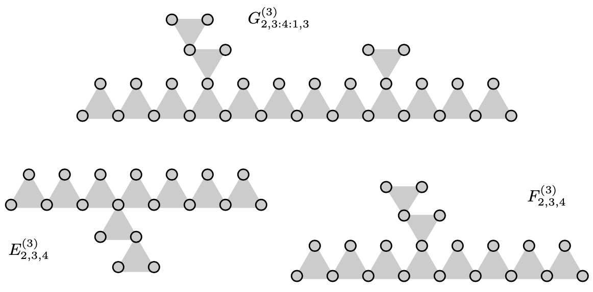
Figure 6. Examples of hypergraphs of type $E_{i,j,k}^{(3)}$, $F_{i,j,k}^{(3)}$ and $G^{(3)}_{i,j:k:l,t}$.

Apart from $C_{2}^{(3)}$, for all uniform hypergraphs defined in the rest of this section, we assume that adjacent edges has just one vertex in common. The $3$-uniform graphs $E^{(3)}_{i,j,k}$, $F^{(3)}_{i,j,k}$ and $G^{(3)}_{i,j:k:l,t}$ are respectively obtained:

• by attaching three hyperpaths of length $i,j,k$ to one vertex;

• by attaching three hyperpaths of length $i,j,k$ to each vertex of a fixed edge;

• by attaching four hyperpaths of length $i,j,l,t$ to four ending vertices of a hyperpath $A^{(3)}_{k+2}$ of length $k+2\geqslant 2$ (see Fig. 6).

To make notation consistent with the $r=2$ case, we set: $E^{(3)}_{6}:=E^{(3)}_{1,2,2}$, $E^{(3)}_{7}:=E^{(3)}_{1,2,3},E^{(3)}_{8}:=E^{(3)}_{1,2,4},\tilde{E}^{(3)}_{6}:=E^{(3)}_{2,2,2},\tilde{E}^{(3)}_{7}:=E^{(3)}_{1,3,3}$, $\tilde{E}^{(3)}_{8}:=E^{(3)}_{1,2,5}$, and $D^{(3)}_{n}:=E^{(3)}_{1,1,n-2}$.

We are now in the stage to describe the elements in $\mathcal{G}_{\mathcal{A}}^{\rho_{r}}$ and in $\mathcal{G}_{\mathcal{A}}^{<\rho_{r}}$. Lu and Man [31] first characterized the $3$-uniform hypergraphs in the two sets, finding the $r$-uniform hypergraphs for $r\geqslant 4$ at a later time.

Theorem 8.2.

[31] Let $\rho_{3}=\sqrt[3]{4}$. If a $3$-uniform hypergraph $H$ belongs to $\mathcal{G}_{\mathcal{A}}^{<\rho_{3}}$, then it is one of the following graphs:

• the hyperpath $A^{(3)}_{m}$ of $m\geqslant 1$ edges.
  

• $D^{(3)}_{m}$ for $m\geqslant 3$;
  

• $D^{\prime(3)}_{m}:=F^{(3)}_{1,1,m-3}$ for $m\geqslant 4$;
  

• $B^{(3)}_{m}=F^{(3)}_{1,2,m-4}$ for $m\geqslant 5$;
  

• $B^{\prime(3)}_{m}:=G^{(3)}_{1,1:(m-6):1,1}$ for $m\geqslant 6$;
  

• $\overline{B}^{(3)}_{m}:=G^{(3)}_{1,1:(n-7):1,2}$ for $m\geqslant 7$;
  

• $BD^{(3)}_{m}$ for $m\geq 5$ (see Fig. 7);
  

• Thirty-one exceptional 3-uniform hypergraphs: $E^{(3)}_{6}$; $E^{(3)}_{7}$; $E^{(3)}_{8}$; $F^{(3)}_{1,3,k}$ (for $3\leqslant k\leqslant 13$); $F^{(3)}_{1,4,k}$ (for $4\leqslant k\leqslant 7$); $F^{(3)}_{1,5,5}$; $F^{(3)}_{2,2,k}$ (for $2\leqslant k\leqslant 6$); $F^{(3)}_{2,3,3}$; and $G^{(3)}_{1,1:k:1,3}$ (for $0\leqslant k\leqslant 5$).

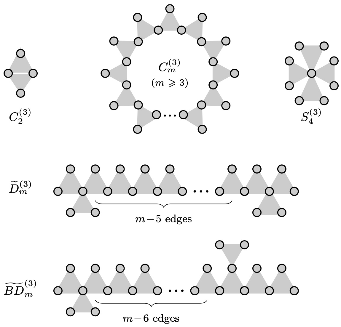
Figure 7. Some hypergraphs involved in Theorems 8.2 and 8.3.

Theorem 8.3.

[31] Let $\rho_{3}=\sqrt[3]{4}$. If a $3$-uniform hypergraph $H$ belongs to ${\mathcal{G}}_{\mathcal{A}}^{\rho_{3}}$, then $H$ is one of the following hypergraphs:

• the hypercycle $C^{(3)}_{m}$ for $m\geqslant 3$;
  

• $\tilde{D}^{(3)}_{m}$ for $m\geq 5$;
  

• $\tilde{B}^{(3)}_{m}:=G^{(3)}_{1,2:(m-8):1,2}$ for $m\geq 8$;
  

• $\widetilde{BD}^{(3)}_{m}$ for $m\geq 6$ (see Fig. 7);

• Twelve exceptional 3-uniform hypergraphs: $C^{(3)}_{2},S^{(3)}_{4}$, $\tilde{E}^{(3)}_{6},\tilde{E}^{(3)}_{7}$, $\tilde{E}^{(3)}_{8}$, $F^{(3)}_{2,3,4}$, $F^{(3)}_{2,2,7}$, $F^{(3)}_{1,5,6}$, $F^{(3)}_{1,4,8}$, $F^{(3)}_{1,3,14}$, $G^{(3)}_{1,1:0:1,4}$, and $G^{(3)}_{1,1:6:1,3}$. (see Fig. 6 and 7.)

A hypergraph $H=(V,E)$ is called reducible if every edge $e$ contains at least one leaf vertex $v_{e}$. In this case, we can define an $(r-1)$-uniform multi-hypergraph $H=(V,E)$ by removing $v_{e}$ from each edge $e$, i.e., $V^{\prime}=V\backslash\{v_{e}|e\in E\}$ and $E=\{e-v_{e}|e\in E\}$. We say that $H^{\prime}$ is reduced from $H$, whereas $H$ extends $H^{\prime}$. As proved in [31], If $H$ extends $H^{\prime}$, then $H\in\mathcal{G}_{\mathcal{A}}^{\rho_{r}}$ (resp., $H\in\mathcal{G}_{\mathcal{A}}^{<\rho_{r}}$) if and only if $H^{\prime}\in\mathcal{G}_{\mathcal{A}}^{\rho_{r-1}}$ (resp., $H^{\prime}\in\mathcal{G}_{\mathcal{A}}^{<\rho_{r-1}}$).

Theorem 8.4.

[31] Let $r\geqslant 4$ and $\rho_{r}=\sqrt[r]{4}$. If an $r$-uniform hypergraphs lies in $\mathcal{G}_{\mathcal{A}}^{<\rho_{r}}$, then it must be one of following graphs:

• $A^{(r)}_{n}$, $D^{(r)}_{n}$, $D^{\prime(r)}_{n}$, $B^{(r)}_{n}$, $B^{\prime(r)}_{n}$, $\bar{B}^{(r)}_{n}$, $BD^{(r)}_{n}$, $E^{(r)}_{6}$, $E^{(r)}_{7},E^{(r)}_{8}$, $F^{(r)}_{2,3,3}$, $F^{(r)}_{2,2,j}$ (for $2\leqslant j\leqslant 6$), $F^{(r)}_{1,3,j}$ (for $3\leqslant j\leqslant 13$), $F^{(r)}_{1,4,j}$ (for $4\leqslant j\leqslant 7$), $F^{(r)}_{1,5,5}$, and $G^{(r)}_{1,1:j:1,3}$ (for $0\leqslant j\leq 5$). These are the $r$-uniform hypergraphs obtained by extending $r-3$ times the hypergraphs in the list of Theorem 8.2;
  

• $H^{(r)}_{1,1,1,1}$, $H^{(r)}_{1,1,1,2}$, $H^{(r)}_{1,1,1,3}$, $H^{(r)}_{1,1,1,4}$. These are the $r$-uniform hypergraphs obtained by extending $r-4$ times the hypergraphs in Fig. 8.

Figure 8. Some hypergraphs involved in Theorems 8.4 and 8.5.

Theorem 8.5.

[31] Let $r\geq 4$ and $\rho_{r}=\sqrt[r]{4}$. If an $r$-uniform hypergraph $H$ belongs to $\mathcal{G}_{\mathcal{A}}^{\rho_{r}}$, then $H$ must be one of the following graphs:

• $C^{(r)}_{n}$, $\tilde{D}^{(r)}_{n}$, $\tilde{B}^{(r)}_{n}$, $\widetilde{BD}^{(r)}_{n}$, $C^{(r)}_{2}$, $S^{(r)}_{4}$, $\tilde{E}^{(r)}_{6}$, $\tilde{E}^{(r)}_{7}$, $\tilde{E}^{(r)}_{8}$, $F^{(r)}_{2,3,4}$, $F^{(r)}_{2,2,7}$, $F^{(r)}_{1,5,6}$, $F^{(r)}_{1,4,8}$,$F^{(r)}_{1,3,14}$, $G^{(r)}_{1,1:0:1,4}$, and $G^{(r)}_{1,1:6:1,3}$. These are the $r$-uniform hypergraphs obtained by extending $r-3$ times the hypergraphs in the list of Theorem 8.3;

• the hypergraph $H^{(r)}_{1,1,2,2}$ obtained by extending $r-4$ times the hypergraph $H^{(4)}_{1,1,2,2}$ in Fig. 8.

Taken a careful look to the proofs in [31], our experience suggests that the next considerable limit point for $\mathcal{A}$-spectral radius of connected $r$-uniform hypergraphs should be the number $\sqrt[r]{2+\sqrt{5}}$.

Problem 4.

For the adjacency tensors of connected $r$-uniform hypergraphs,

• determine the limit points of $\mathcal{A}$-spectral radius less than $\sqrt[r]{2+\sqrt{5}}$, and further identify all of them;

• establish whether each real number exceeding $\sqrt[r]{2+\sqrt{5}}$ is an $\mathcal{A}$-limit point;

• characterize the $r$-uniform hypergraphs whose $\mathcal{A}$-spectral radius is at most $\sqrt[r]{2+\sqrt{5}}$.

Other interesting fields of investigation are the signless Laplacian tensor and Laplacian tensor of the uniform hypergraph $H$, defined as $\mathcal{Q}(H)=\mathcal{D}(H)+\mathcal{A}(H)$ and $\mathcal{L}(H)=\mathcal{D}(H)-\mathcal{A}(H)$, where $\mathcal{D}(H)$ is the diagonal tensor of order $k$ and dimension $n$, whose diagonal entry $D_{ii\ldots i}$ is the degree of the vertex $i$ for all $i\in[n]$ (see [39]). As far as we know, the Hoffman program with respect to these two tensors haven’t yet been studied. Results concerning the Hoffman program for the (signless) Laplacian matrices in Sections 3 and 4 bring us to pose the following problem.

Problem 5.

For the Laplacian and the signless Laplacian tensors of connected $r$-uniform hypergraphs,

• prove that the smallest limit point of the $\{\mathcal{L},\mathcal{Q}\}$-spectral radius is $\sqrt[r]{16}$.

• characterize the $r$-uniform hypergraphs with $\{\mathcal{L},\mathcal{Q}\}$-spectral radius at most $\sqrt[r]{16}$.

• determine the $\{\mathcal{L},\mathcal{Q}\}$-limit points which are less than $\sqrt[r]{2+\varepsilon}$;

• establish whether each real number exceeding $\sqrt[r]{2+\varepsilon}$ is an $\{\mathcal{L},\mathcal{Q}\}$-limit point; where $\varepsilon=\frac{{\;}1{\;}}{3}\left((54-6\sqrt{33})^{\frac{{\;}1{\;}}{3}}+(54+6\sqrt{33})^{\frac{{\;}1{\;}}{3}}\right)$ like in Section 2.

• characterize the $r$-uniform hypergraphs with $\{\mathcal{L},\mathcal{Q}\}$-spectral radius at most $\sqrt[r]{2+\sqrt{5}}$.

9. $A_{\alpha}$-matrix

Nikiforov [33] defined the $A_{\alpha}$-matrix of a graph $G$ to be the convex linear combination

$$A_{\alpha}(G)=\alpha D(G)+(1-\alpha)A(G),\quad\alpha\in[0,1].$$

Such matrix not only merges the $A$-spectra and $Q$-spectra, but offer a different perspective to generalize and deepen the spectral properties of graphs. Clearly,

$$A(G)=A_{0}(G),\;\;Q(G)=2A_{1/2}(G),\;\;\text{and}\;\;L(G)=\frac{1}{\alpha-\beta}(A_{\alpha}(G)-A_{\beta}(G))\;\;\text{ for all $\alpha\not=\beta$}.$$

An interesting literature on Nikiforov’s matrix is growing rapidly; from the subsequent papers by Nikiforov et al. [34, 35] to the recent applications to signed, mixed and gain graphs [3, 28], there are already more than fifty published papers on the spectral properties of the $A_{\alpha}$-matrix.

A first attempt to study the limit points of the $A_{\alpha}$-spectral radius of graphs has been already performed.

Theorem 9.1.

[50] The smallest $A_{\alpha}$-limit point for the $A_{\alpha}$-spectral radius of graphs is $2$.

The connected graphs with $A_{\alpha}$-index at most $2$ are also characterized. In Theorem 9.2, the following four numbers are of considerable importance:

$$s_{1}=\dfrac{4}{n+1+\sqrt{(n+1)^{2}-16}};$$

the root $s_{2}=0.2192+$ of the polynomial $2\alpha^{3}-11\alpha^{2}+16\alpha-3$; the root $s_{3}=0.1206+$ of $\alpha^{3}-6\alpha^{2}+9\alpha-1$; and the root $s_{4}=0.0517+$ of $2\alpha^{3}-13\alpha^{2}+20\alpha-1$.

Theorem 9.2.

[50] Let $G$ be a connected graph with order $n$, and let $\alpha\in[0,1]$. The following two statements hold.

• $\rho_{A_{\alpha}}(G)<2$ if and only if $G$ is one of the following graphs:

  • $P_{n}$ ($n\geq 1$) for $\alpha\in[0,1)$;

  • $T_{1,1,n-3}$ ($n\geq 4$) for $\alpha\in[0,s_{1})$;

  • $T_{1,2,2}$ for $\alpha\in[0,s_{2})$, $T_{1,2,3}$ for $\alpha\in[0,s_{3})$ and $T_{1,2,4}$ for $\alpha\in[0,s_{4})$.

• $\rho_{A_{\alpha}}\!(G)=2$ if and only if $G$ is one of the following graphs:

  • $C_{n}$, $n\geq 3$;

  • $P_{n}$ ($n\geq 3$) for $\alpha=1$;

  • $W_{n}\;(n\geq 6)$ for $\alpha=0$;

  • $T_{1,1,n-3}$ for $\alpha=s_{1}$;

  • $T_{1,2,2}$ for $\alpha=s_{2}$, $T_{1,2,3}$ for $\alpha=s_{3}$, $T_{1,2,4}$ for $\alpha=s_{4}$;

  • $T_{1,3,3}$, $T_{1,2,5}$, $K_{1,4}$ and $T_{2,2,2}$, for $\alpha=0$.

The Hoffman program for the adjacency and the signless Laplacian matrix suggests that a natural second step is to identify all the possible $A_{\alpha}$-limit points which are bigger than $2$. In view of this goal, it is necessary to investigate the $A_{\alpha}$-spectral properties of graphs in the first instance. We do this in Subsection 9.1, whereas we find in Subsection 9.2 many $A_{\alpha}$-limit points larger than $2$ related to suitably built sequences of graphs which already turned out to be useful to detect the important $L$-limit point $\omega$ (see [17] and Section 3).

9.1. Some general results on the $A_{\alpha}$-matrix

We start by fixing some notation. Let $u$ and $v$ be two vertices of a connected graph $G$. As usual, we denote by $N_{G}(u)$ the neighbourhood of $u$ in $G$, i.e. the set of vertices in $V(G)$ adjacent to $u$, and by $d(u,v)$ the number of edges in a shortest path connecting $u$ and $v$. Throughout this section, we write the matrices $A_{\alpha}(P_{n})$ and $A_{\alpha}(C_{n})$ according to vertex labellings $u_{1},\dots,u_{n}\in V(P_{n})$ and $v_{1},\dots,v_{n}\in V(C_{n})$ such that $u_{i}$ (resp. $v_{i}$) is adjacent to $u_{i-1}$ and $u_{i+1}$ (resp., $v_{i-1}$ and $v_{i+1}$) for $2\leqslant i\leqslant n-1$.

Lemma 9.3.

[33] For every connected graph $G$ with maximum vertex degree $\Delta$, and for every $\alpha\in[0,1]$, the $A_{\alpha}$-spectral radius $\rho\!_{{}_{A_{\alpha}}}(G)$ satisfies the following properties:

:

• $\frac{1}{2}\left(\alpha(\Delta+1)+\sqrt{\alpha^{2}(\Delta+1)^{2}+4\Delta(1-2\alpha)}\right)\leqslant\rho\!_{{}_{A_{\alpha}}}\!(G)\leqslant\Delta$;

• if $H$ is a proper subgraph of $G$, then $\rho\!_{{}_{A_{\alpha}}}\!(H)<\rho\!_{{}_{A_{\alpha}}}\!(G)$;

• if $0\leqslant\alpha<\beta\leqslant 1$, then $\rho\!_{{}_{A_{\alpha}}}\!(G)<\rho\!_{{}_{A_{\beta}}}\!(G)$.

Lemma 9.4.

[34] The $A_{\alpha}$-spectral radius of the path $P_{n}$ satisfies the following inequalities.

• $\displaystyle\rho\!_{{}_{A_{\alpha}}}\!(P_{n})\leqslant\begin{cases}\small 2\alpha+2(1-\alpha)\cos(\frac{\pi}{n+1})&\text{for $\alpha\in[0,1/2)$,}\\[8.00003pt] 2\alpha+2(1-\alpha)\cos(\frac{\pi}{n})&\text{for $\alpha\in[1/2,1]$.}\end{cases}$

  Equality holds if and only if $\alpha=0$, $\alpha=1/2$, $\alpha=1$.
  

• $\displaystyle\rho\!_{{}_{A_{\alpha}}}\!(P_{n})\geqslant\begin{cases}2\alpha+2(1-\alpha)\cos(\frac{\pi}{n})&\text{for $\alpha\in[0,1/2)$}\\[8.00003pt] 2\alpha+2\alpha\cos(\frac{\pi}{n})-2(2\alpha-1)\cos(\frac{\pi}{n+1})&\text{for $\alpha\in[1/2,1]$.}\\ \end{cases}$

  Equality holds if and only if $\alpha=1/2$.

Let $\phi(G)=\det(\lambda I-A_{\alpha}(G))$ denote the $A_{\alpha}$-polynomial of a graph $G$. For every vertex $v\in V(G)$, we indicate by $A_{\alpha}(G)_{v}$ the principal submatrix of $A_{\alpha}(G)$ obtained by deleting the row and the column corresponding to the vertex $v$, and by $\phi(G)_{v}$ the characteristic polynomial of $A_{\alpha}(G)_{v}$.

Lemma 9.5.

[9] The $A_{\alpha}$-characteristic polynomial of $G=G_{1}u\!\!:\!\!vG_{2}$, the graph obtained by joining the vertex $u$ of the graph $G_{1}$ to the vertex $v$ of the graph $G_{2}$ by an edge, is given by the following formula.

$$\phi(G)=\phi(G_{1})\phi(G_{2})-\alpha\phi(G_{1})_{u}\phi(G_{2})-\alpha\phi(G_{1})\phi(G_{2})_{v}+(2\alpha-1)\phi(G_{1})_{u}\phi(G_{2})_{v}.$$

For each positive integer $n$, we consider the matrix $B_{n}$ obtained from $A_{\alpha}(P_{n+1})$ by deleting the row and column corresponding to the end vertex $u_{1}$ of the path $P_{n+1}$, and the matrix $H_{n}$ obtained from $A_{\alpha}(P_{n+2})$ by deleting the rows and the columns corresponding to both end-vertices of $P_{n+2}$. Clearly, both $B_{n}$ and $H_{n}$ are $n\times n$ matrices. We explicitly observe that the three matrices $P_{n}$, $B_{n}$ and $H_{n}$ are equal if and only if $\alpha=0$.

For every $\alpha\in[0,1)$, we also set

$$\phi(P_{0})=\frac{1-2\alpha}{(1-\alpha)^{2}},\quad\phi(B_{0})=1,\quad\text{and}\quad\phi(H_{0})=1.$$

Lemma 9.6.

The equation

(4) $$\left(\lambda+\frac{1}{\alpha}-2\right)\phi(B_{n})=\phi(P_{n+1})+\frac{(1-\alpha)^{2}}{\alpha}\,\phi(P_{n})$$

holds for every $n\geqslant 0$ and $\alpha\in(0,1)$.

Proof.

For $n\in\{0,1\}$, the statement follows from a direct calculation. For $n>1$, the matrix $B_{n}$ has the form

(5) $$\left(\begin{array}[]{cccccc}\lambda-2\alpha&\alpha-1&0&\cdots&0\\ \alpha-1&\lambda-2\alpha&\alpha-1&\cdots&0\\ 0&\alpha-1&\lambda-2\alpha&\cdots&0\\ \vdots&\vdots&\vdots&\ddots&\vdots\\ 0&0&0&\cdots&\lambda-\alpha\\ \end{array}\right).$$

The first row of (5) is equal to the sum $(\lambda-\alpha,\alpha-1,0,\dots 0)+(-\alpha,0,\dots 0)$. By linearity of the determinant function in the first row, we get

(6) $$\phi(B_{n})=\phi(P_{n})-\alpha\phi(B_{n-1}).$$

We now use Lemma 9.5, in the case $G_{1}=P_{n}$, $u$ is an end vertex of $G_{1}$, and $G_{2}=P_{1}$. Clearly, $G_{1}u\!:\!vG_{2}=P_{n+1}$ and

(7) $$\phi(P_{n+1})=(\lambda-\alpha)\phi(P_{n})+(2\alpha-\alpha\lambda-1)\phi(B_{n-1}).$$

Combining (6) and (7), we arrive at (4). ∎

Lemma 9.7.

For every $n\geqslant 1$ and $\alpha\in[0,1)$, the following equalities hold.

• $\phi(P_{n+1})=(\lambda-2\alpha)\phi(P_{n})-(1-\alpha)^{2}\phi(P_{n-1})$;

• $\phi(P_{n+1})=\lambda\phi(H_{n})+(2\alpha-1)\phi(H_{n-1})$;

• $\phi(C_{n+2})=(x-2\alpha)\phi(H_{n+1})-2(\alpha-1)^{2}\phi(H_{n})+2(-1)^{n+1}(\alpha-1)^{n+2}$.

Proof.

For $n=1$, (i) and (ii) follow from a direct calculation. Let now $n>1$. A cofactor expansion along the row corresponding to an end vertex of $P_{n+1}$ suffices to show that (i) holds for $\alpha=0$. For $\alpha>0$, (i) follows from (4) and (7).

We now prove (ii) for $n>1$. By expanding the determinant $\phi(H_{n+1})$ by the first row we get

(8) $$\phi(H_{n+1})=(\lambda-2\alpha)\phi(H_{n})-(1-\alpha)^{2}\phi(H_{n-1}).$$

Once we write the first and the last row of $A_{\alpha}(P_{n+1})$ as $(\lambda-2\alpha,\alpha-1,0,\dots 0)+(\alpha,0,\dots,0)$ and $(0,\dots,0,\alpha-1,\lambda-2\alpha)+(0,\dots,0,\alpha)$, linearity of the determinant function in the first and in the last row gives

$$\phi(P_{n+1})=\phi(H_{n+1})+2\alpha\phi(H_{n})+\alpha^{2}\phi(H_{n-1})$$

which, together with (8), leads to (ii).

For (iii), we consider the cofactor expansion of $\phi(C_{n+2})$ along the first row, getting

$$\begin{split}\phi(C_{n+2})&=\left|\begin{array}[]{cccccc}\lambda-2\alpha&\alpha-1&0&\cdots&\alpha-1\\ \alpha-1&\lambda-2\alpha&\alpha-1&\cdots&0\\ 0&\alpha-1&\lambda-2\alpha&\cdots&0\\ \vdots&\vdots&\vdots&\ddots&\vdots\\ \alpha-1&0&0&\cdots&\lambda-2\alpha\\ \end{array}\right|\\ &=(\lambda-2\alpha)\phi(H_{n+1})-(\alpha-1)\left|\begin{array}[]{cccccc}\alpha-1&&\alpha-1&\cdots&0\\ 0&&\lambda-2\alpha&\cdots&0\\ \vdots&&\vdots&\ddots&\vdots\\ \alpha-1&&0&\cdots&\lambda-2\alpha\\ \end{array}\right|-(\alpha-1)^{2}\phi(H_{n})+(-1)^{n+3}(\alpha-1)^{n+2}\\ &=(\lambda-2\alpha)\phi(H_{n+1})-(\alpha-1)^{2}\phi(H_{n})+(-1)^{n+3}(\alpha-1)^{n+2}-(\alpha-1)^{2}\phi(H_{n})+(-1)^{n+3}(\alpha-1)^{n+2}\\ &=(\lambda-2\alpha)\phi(H_{n+1})-2(\alpha-1)^{2}\phi(H_{n})+2(-1)^{n+3}(\alpha-1)^{n+2}.\end{split}$$

This finishes the proof, since $n+1$ and $n+3$ have the same parity. ∎

Throughout the rest of the paper, we shall make use of the following notations:

(9) $$\Delta_{\lambda,\alpha}=\sqrt{(\lambda-4\alpha+2)(\lambda-2)}\qquad\text{and}\qquad h(\lambda)_{\alpha}=\frac{\lambda-\Delta_{\lambda,\alpha}}{2\alpha(\lambda-2)+2}.$$

Proposition 9.8.

Let $n$ be any non-negative integer. After setting

$$s=\frac{\lambda-2\alpha+\Delta_{\lambda,\alpha}}{2},\qquad\text{and}\qquad t=\frac{\lambda-2\alpha-\Delta_{\lambda,\alpha}}{2},$$

Equalities (i), (ii) and (iv) below hold for $\alpha\in[0,1)$. Equality (iii) holds for $\alpha\in(0,1)$.

• $\phi(H_{n})=\Delta_{\lambda,\alpha}^{-1}(s^{n+1}-t^{n+1});$

• $\phi(P_{n+1})=\Delta_{\lambda,\alpha}^{-1}((s+\alpha)^{2}s^{n}-(t+\alpha)^{2}t^{n});$

• $\phi(B_{n+1})=$$\displaystyle\frac{1}{\Delta_{\lambda,\alpha}}\cdot\frac{\alpha}{\left(\alpha(\lambda-2)+1\right)}\left((s+\alpha)^{2}\left(s+\frac{(1-\alpha)^{2}}{\alpha}\right)s^{n}-(t+\alpha)^{2}\left(t+\frac{(1-\alpha)^{2}}{\alpha}\right)t^{n}\right).$

• $\displaystyle\lim\limits_{n\rightarrow\infty}\frac{\phi(B_{n-1})}{\phi(P_{n})}=\lim\limits_{n\rightarrow\infty}\frac{\phi(H_{n-2})}{\phi(B_{n-1})}=h(\lambda)_{\alpha}$.

Proof.

We start by noticing that $s$ and $t$ are the roots of the polynomial $x^{2}-(\lambda-2\alpha)x+(1-\alpha)^{2}.$ Result (i) surely holds for $n\in\{0,1\}$. We now argue by induction on $n$. Suppose that $n\geqslant 1$. From (8) and induction, it follows that

$$\begin{split}\phi(H_{n+1})&=(\lambda-2\alpha)\phi(H_{n})-(1-\alpha)^{2}\phi(H_{n-1})\\ &=(\lambda-2\alpha)\Delta_{\lambda,\alpha}^{-1}(s^{n+1}-t^{n+1})-(1-\alpha)^{2}\Delta_{\lambda,\alpha}^{-1}(s^{n}-t^{n})\\ &=\Delta_{\lambda,\alpha}^{-1}((\lambda-2\alpha)s-(1-\alpha)^{2})s^{n}-\Delta_{\lambda,\alpha}^{-1}((\lambda-2\alpha)t-(1-\alpha)^{2})t^{n}\\ &=\Delta_{\lambda,\alpha}^{-1}(s^{n+2}-t^{n+2}).\end{split}$$

Now that we know that (i) holds, Equalities (ii) and (iii) come from Lemma 9.7(ii) and Lemma 9.6 respectively, once we note that, by definition, $s$ and $t$ both satisfy

$$\lambda x+2\alpha-1=(x+\alpha)^{2}.$$

In order to prove (iv), the following identities turn out to be useful:

(10) $$st=(1-\alpha)^{2};\qquad\frac{t+\alpha}{a(\lambda-2)+1}=h(\lambda)_{\alpha},\qquad\text{and}\qquad\frac{1}{(s+\alpha)^{2}}=\left(h(\lambda)_{\alpha}\right)^{2}.$$

It is also important to note that $\lim_{n\rightarrow\infty}\left(t/s\right)^{n}=0,$ since $t<s$. The cases $\alpha=0$ and $\alpha\in(0,1)$ will be dealt separately. If $\alpha=0$, by definition we have $\phi(P_{n})=\phi(B_{n})=\phi(H_{n})$. Therefore, from (ii) we get

$$\scalebox{1.0}{\mbox{$\displaystyle\lim\limits_{n\rightarrow\infty}\frac{\phi(B_{n-1})}{\phi(P_{n})}=\lim\limits_{n\rightarrow\infty}\frac{\phi(P_{n-1})}{\phi(P_{n})}=\lim\limits_{n\rightarrow\infty}\frac{s^{n+1}-t^{n+1}}{s^{n+2}-t^{n+2}}=\frac{1}{s}\lim\limits_{n\rightarrow\infty}\frac{1-\left(\frac{t}{s}\right)^{n+1}}{1-\left(\frac{t}{s}\right)^{n+2}}=\frac{1}{s}=t=h(\lambda)_{0}$}},$$

and, similarly,

$$\lim\limits_{n\rightarrow\infty}\frac{\phi(H_{n-2})}{\phi(B_{n-1})}=\lim\limits_{n\rightarrow\infty}\frac{\phi(P_{n-2})}{\phi(P_{n-1})}=t=h(\lambda)_{0}$$

as claimed. Let now $\alpha\in(0,1)$. Using (ii) and (iii), we obtain

For the last equality, we have used the second identity in (10). We now compute

where, for the last equality, we have used the second and the third identity in (10). ∎

According to [22], an internal path of a graph $G$ is a walk $v_{0}v_{1}\dots v_{k}$ (here $k\geqslant 1$), where the vertices $v_{1},\dots,v_{k}$ are pairwise distinct, $d(v_{0})>2$, $d(v_{k})>2$ and $d(v_{i})=2$ whenever $0<i<k$. We say that an internal path is of type I (resp., type II) if $v_{0}=v_{k}$ (resp., $v_{0}\not=v_{k}$) (see Fig. 9).

Subdividing an edge belonging to an internal paths has well-known $A$-spectral consequences (see [22] or [1, p. 79]). The impact on the $A_{\alpha}$-spectral radius when internal paths are involved is stated in [29]. Proposition 9.9 deals with all cases. We recall that the double snake of order $n\geqslant 6$ is the graph $W_{n}$ depicted in Fig. 1 and 9 containing an internal path of type II $v_{0}\dots v_{n-5}$ such that $d(v_{0})=d(v_{n-5})=3$.

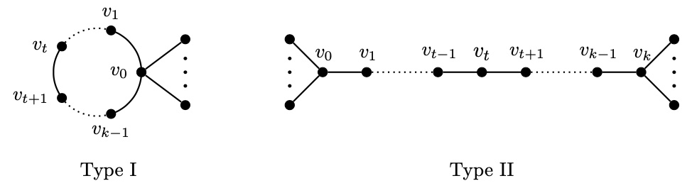
Figure 9. The two types of internal path

Proposition 9.9.

Let $uv$ be an edge of the connected graph $G$, and let $G_{uv}$ be the graph obtained from $G$ by subdividing the edge $uv$ of $G$. Set $\alpha\in[0,1)$.

• $\rho\!_{{}_{A_{\alpha}}}\!(C_{n})=2$ and $\rho\!_{{}_{A_{0}}}\!(W_{n})=2$;

• If $(G,\alpha)\neq(C_{n},\alpha)$ and $uv$ is not in an internal path of $G$, then $\rho\!_{{}_{A_{\alpha}}}\!(G_{uv})>\rho\!_{{}_{A_{\alpha}}}\!(G)$;

• If $(G,\alpha)\neq(W_{n},0)$ and $uv$ belongs to an internal path of $G$, then $\rho\!_{{}_{A_{\alpha}}}\!(G_{uv})<\rho\!_{{}_{A_{\alpha}}}\!(G)$.

Proof.

It is straightforward to show that the $A_{\alpha}$-spectral radius of a regular graph $G$ is the degree of $G$ [33, Section 3.2]; hence, $\rho_{A_{\alpha}}(C_{n})=2$. The latter of (i) follows from [22].

In the hypotheses of (ii), it is not hard to show that $G_{uv}$ contains a proper subgraph isomorphic to $G$. Therefore, by Lemma 9.3(ii) we get $\rho\!_{{}_{A_{\alpha}}}\!(G_{uv})>\rho\!_{{}_{A_{\alpha}}}\!(G)$.

For (iii), we refer the reader to the proof of Lemma 1.1 in [29], with the warning that in such proof the authors assume that $G$ properly contains a double snake. What is really crucial is their argument is that $\rho\!_{{}_{A_{\alpha}}}\!(G)>2$, and this is true whenever $G$ contains an internal path of any type and $(G,\alpha)\neq(W_{n},0)$. In fact, from Lemmas 3.1(ii) and 3.2(ii) in [50], it follows that $\rho\!_{{}_{A_{\alpha}}}\!(W_{n})>2$ if and only if $\alpha\neq 0$; moreover, if $G$ contains an internal path of type I, a fortiori it contains a cycle $C_{r}$ as a proper subgraph; therefore, using (i) together with Lemma 9.3(ii), we immediately get $\rho\!_{{}_{A_{\alpha}}}\!(G)>\rho\!_{{}_{A_{\alpha}}}\!(C_{r})=2$. ∎

9.2. Limit points for the $A_{\alpha}$-spectral radius of compound graphs

Let $v$ be an end vertex of the path $P_{n}$, and let $u$ be a vertex of a graph $G$ vertex-disjoint with respect to $P_{n}$. We denote by $G_{u}(P_{n})$ the graph $Gu\!:\!vP_{n}$. Recall that $V(G_{u}(P_{n}))=V(G)\cup V(P_{n})$ and $E(G_{u}(P_{n}))=E(G)\cup E(P_{n})\cup\{uv\}$.

Proposition 9.10.

The $A_{\alpha}$-spectral radius of the graph sequence $\{G_{u}(P_{n})\}_{n\in\mathbb{N}}$ has a limit point $\chi_{u}(G)\geqslant 2$. If $\chi_{u}(G)>2$, then $\chi_{u}(G)$ is the largest root of the equation

$$\left(1-\alpha\cdot h(\lambda)_{\alpha}\right)\phi(G)-\left(\alpha-(2\alpha-1)\cdot h(\lambda)_{\alpha}\right)\phi(G)_{u}=0,$$

where $h(\lambda)_{\alpha}$ is defined in (9).

Proof.

The inequalities

$$\rho\!_{{}_{A_{\alpha}}}\!(G_{u}(P_{n}))<\rho\!_{{}_{A_{\alpha}}}\!(G_{u}(P_{n+1}))\qquad\text{and}\qquad\rho\!_{{}_{A_{\alpha}}}\!(G_{u}(P_{n}))\leqslant\Delta(G_{u}(P_{n}))$$

both come from Lemma 9.3. Altogether, they imply that $\lim_{n\rightarrow\infty}\rho\!_{{}_{A_{\alpha}}}\!(G_{u}(P_{n}))=\chi_{u}(G)$ exists. If $G_{u}(P_{n})$ is a path, then by Lemma 9.4, we get $\chi_{u}(G)=2$. Since $G_{u}(P_{n})$ properly contains $P_{n}$, then $\rho\!_{{}_{A_{\alpha}}}\!(G_{u}(P_{n}))>\rho\!_{{}_{A_{\alpha}}}\!(P_{n})$; hence, $\chi_{u}(G)\geqslant 2$.

Suppose now $\chi_{u}(G)>2$. From Lemma 9.5 we get

(11) $$\begin{split}\phi(G_{u}(P_{n}))&=\phi(G)\phi(P_{n})-\alpha\phi(G)_{u}\phi(P_{n})-\alpha\phi(G)\phi(B_{n-1})+(2\alpha-1)\phi(G)_{u}\phi(B_{n-1})\\[5.69046pt] &=\phi(P_{n})\left(\left(1-\alpha\frac{\phi(B_{n-1})}{\phi(P_{n})}\right)\phi(G)-\left(\alpha-(2\alpha-1)\frac{\phi(B_{n-1})}{\phi(P_{n})}\right)\phi(G)_{u}\right).\end{split}$$

Since $\chi_{u}(G)>2$ and $\rho\!_{{}_{A_{\alpha}}}\!(P_{n})\leqslant 2$, then $\chi_{u}(G)$ is the largest positive root of the following equation:

$$\lim\limits_{n\rightarrow\infty}\left(\left(1-\alpha\frac{\phi(B_{n-1})}{\phi(P_{n})}\right)\phi(G)-\left(\alpha-(2\alpha-1)\frac{\phi(B_{n-1})}{\phi(P_{n})}\right)\phi(G)_{u}\right)=0,$$

and Proposition 9.8(iv) ensures that $\displaystyle\lim\limits_{n\rightarrow\infty}\phi(B_{n-1})/\phi(P_{n})=h(\lambda)_{\alpha}$. ∎

Corollary 9.11.

Let $u$ be the vertex in of degree 3 in $K_{1,3}$. Then,

$$\lim\limits_{n\rightarrow\infty}\rho\!_{{}_{A_{\alpha}}}\!((K_{1,3})_{u}(P_{n}))=\frac{1}{2}\left(5\alpha+3\sqrt{2-4\alpha+3\alpha^{2}}\right).$$

Proof.

Lemma 9.3 and a direct calculation guarantee that, for all $n\geqslant 2$,

$$\rho\!_{{}_{A_{\alpha}}}\!(K_{1,3}(P_{n}))\geqslant\rho\!_{{}_{A_{0}}}\!(K_{1,3}(P_{n}))\geqslant\rho\!_{{}_{A_{0}}}\!(K_{1,3}(P_{2}))>2.$$

Therefore, from Proposition 9.10, it follows that $\lim\limits_{n\rightarrow\infty}\rho\!_{{}_{A_{\alpha}}}\!(K_{1,3}(P_{n}))$ is the largest root of the following equation:

$$\left(1-\alpha h(\lambda)_{\alpha}\right)\phi(K_{1,3})-\left(\alpha-(2\alpha-1)\cdot h(\lambda)_{\alpha}\right)\phi(K_{1,3})_{u}=0.$$

Plugging into the equation above

$$\phi(K_{1,3})=(\lambda-\alpha)^{2}(\lambda^{2}-4\alpha\lambda+6\alpha-3)\qquad\text{and}\qquad\phi(K_{1,3})_{u}=(\lambda-\alpha)^{3},$$

we find that the largest root of the above equation is $\displaystyle\frac{1}{2}\left(5\alpha+3\sqrt{2-4\alpha+3\alpha^{2}}\right)$. ∎

Let $2P_{n}$ be the disjoint union of two copies of $P_{n}$ and let $u_{1},u_{2}\in V(2P_{n})$ be end-vertices belonging to different components. For every non-trivial connected graph $G$ and every $u\in V(G)$, we consider the graph $G_{u}(P_{n},P_{n})$ obtained by adding to $G\cup 2P_{n}$ the edges $uu_{1}$ and $uu_{2}$.

Proposition 9.12.

The $A_{\alpha}$-spectral radius of the graph sequence $\{G_{u}(P_{n},P_{n})\}_{n\in\mathbb{N}}$ has a limit point $\chi^{\prime}_{u}(G)\geqslant 2$. If $\chi^{\prime}_{u}(G)>2$, then $\chi^{\prime}_{u}(G)$ is the largest root of the equation $\Theta(\lambda)_{G,u,\alpha,\infty}=0$, where

$$\Theta(\lambda)_{G,u,\alpha,\infty}=\left(1-\alpha h(\lambda)_{\alpha}\right)\left(\phi(G)(1-\alpha h(\lambda)_{\alpha})-2\alpha\phi(G)_{u}+2(2\alpha-1)\phi(G)_{u}h(\lambda)_{\alpha}\right),$$

and $h(\lambda)_{\alpha}$ is defined in (9).

Proof.

By Lemma 9.3(i), $\{G_{u}(P_{n},P_{n})\}_{n\in\mathbb{N}}$ is a nested sequence of graphs whose $A_{\alpha}$-spectral radius is limited above by $\Delta(G)+2$. Therefore, $\lim_{n\rightarrow\infty}\rho\!_{{}_{A_{\alpha}}}\!(G_{u}(P_{n},P_{n}))=\chi^{\prime}_{u}(G)$ exists, and $\chi^{\prime}_{u}(G)\geqslant\chi_{u}(G)\geqslant 2$, since $G_{u}(P_{n},P_{n})$ properly contains $G_{u}(P_{n})$, and Proposition 9.12 holds.

Now, by applying twice Lemma 9.5 and using (6) and (11), we get

$$\begin{split}\phi(G_{u}(P_{n},P_{n}))&=\phi(G_{u}(P_{n}))\phi(P_{n})-\alpha\phi(G_{u})\phi(B_{n})\phi(P_{n})\\ &\phantom{=}-\alpha\phi(G_{u}(P_{n}))\phi(B_{n-1})+(2\alpha-1)\phi(G)_{u}\phi(B_{n})\phi(B_{n-1}).\\[8.00003pt] &=\phi(G)(\phi(P_{n})-\alpha\phi(B_{n-1}))^{2}-2\alpha\phi(G)_{u}\phi(P_{n})(\phi(P_{n})-\alpha\phi(B_{n-1}))\\ &\phantom{=}+2(2\alpha-1)\phi(G)_{u}\phi(B_{n-1})(\phi(P_{n})-\alpha\phi(B_{n-1}))\end{split}$$

which is also equal to $\phi(P_{n})^{2}\Theta(\lambda)_{G,u,\alpha,n}$, where

$$\Theta(\lambda)_{G,u,\alpha,n}=\left(1-\alpha\frac{\phi(B_{n-1})}{\phi(P_{n})}\right)\left(\phi(G)\left(1-\alpha\frac{\phi(B_{n-1})}{\phi(P_{n})}\right)-2\alpha\phi(G)_{u}+2(2\alpha-1)\phi(G)_{u}\frac{\phi(B_{n-1})}{\phi(P_{n})}\right).$$

By Lemma 9.3, no roots of $(\phi(P_{n}))^{2}$ are larger than $2$; therefore, if $\chi^{\prime}(G)>2$, such number is the largest positive root of

$$\lim\limits_{n\rightarrow\infty}\Theta(\lambda)_{G,u,\alpha,n}=\Theta(\lambda)_{G,u,\alpha,\infty},$$

where the equality comes from Proposition 9.8(iv). ∎

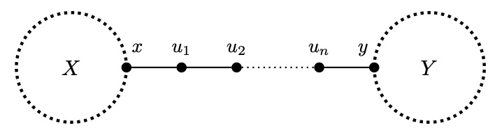
Figure 10. The graph $XY(x,y;n)$

Proposition 9.13.

Let $X$ and $Y$ be two vertex-disjoint connected graphs, and let $G_{n}=XY(x,y;n)$ be the graph obtained by joining $x\in V(X)$ and $y\in V(Y)$ by a path of length $n+1$ (see Fig. 10). Then,

(12) $$\lim\limits_{n\rightarrow\infty}\rho\!_{{}_{A_{\alpha}}}\!(G_{n})=\max\left\{\lim\limits_{n\rightarrow\infty}\rho\!_{{}_{A_{\alpha}}}\!(X_{x}(P_{n})),\lim\limits_{n\rightarrow\infty}\rho\!_{{}_{A_{\alpha}}}\!(Y_{y}(P_{n}))\right\}.$$

Proof.

The existence of $\lim_{n\rightarrow\infty}\rho\!_{{}_{A_{\alpha}}}\!(X_{x}(P_{n}))$ and $\lim_{n\rightarrow\infty}\rho\!_{{}_{A_{\alpha}}}\!(Y_{y}(P_{n}))$ follows from Proposition 9.10(i). We refer the reader to Fig. 10 for notation. If the path $u_{1}u_{2}\dots u_{n}$ is contained in an internal path of $G_{n}$, then from Lemma 9.3(i) and Proposition 9.9(iii) we know that $\lim_{n\rightarrow\infty}\rho\!_{{}_{A_{\alpha}}}\!(G_{n})$ exists. Otherwise, $G_{n}$ is either of type $X_{x}(P_{n+\lvert V(Y)\rvert})$ or $Y_{y}(P_{n+\lvert V(X)\rvert})$. Thus, by Proposition 9.10, $\lim_{n\rightarrow\infty}\rho\!_{{}_{A_{\alpha}}}\!(G_{n})$ exists as well. Since the smallest limit point for the $A_{\alpha}$-spectral radius is $2$ (see [50, Theorem 1.1]), we get

(13) $$2\leqslant\min\left\{\lim\limits_{n\rightarrow\infty}\rho\!_{{}_{A_{\alpha}}}\!(X_{x}(P_{n})),\lim\limits_{n\rightarrow\infty}\rho\!_{{}_{A_{\alpha}}}\!(Y_{y}(P_{n}))\right\}\\ \leqslant\max\left\{\lim\limits_{n\rightarrow\infty}\rho\!_{{}_{A_{\alpha}}}\!(X_{x}(P_{n})),\lim\limits_{n\rightarrow\infty}\rho\!_{{}_{A_{\alpha}}}\!(Y_{y}(P_{n}))\right\}\leqslant\lim\limits_{n\rightarrow\infty}\rho\!_{{}_{A_{\alpha}}}\!(G_{n}),$$

where the third inequality comes from Lemma 9.3(ii). If $\lim_{n\rightarrow\infty}\rho\!_{{}_{A_{\alpha}}}\!(G_{n})=2$, Inequalities (13) imply (12).

If instead $\lim_{n\rightarrow\infty}\rho\!_{{}_{A_{\alpha}}}\!(G)>2$, we use the fact that $G_{n}=(X_{x}(P_{n}))u_{n}\!:\!yY$. Applying Lemma 9.5, we obtain:

where

$$\phi(X_{x}(P_{n}))=\phi(X)\phi(P_{n})-\alpha\phi(X)_{x}\phi(P_{n})-\alpha\phi(X)\phi(B_{n-1})+(2\alpha-1)\phi(X)_{x}\phi(B_{n-1})$$

and

A straightforward algebraic manipulation shows that $\phi(G_{n})=\phi(P_{n})\cdot\Gamma_{n}$, where

By Proposition 9.8(iv), we know that

$$\lim_{n\rightarrow\infty}\phi(B_{n-1})/\phi(P_{n})=\lim_{n\rightarrow\infty}\phi(H_{n-2})/\phi(B_{n-1})=h(\lambda)_{\alpha}.$$

It is now elementary to check that $\lim_{n\rightarrow\infty}\Gamma_{n}$ is the product of

$$\left(1-\alpha\cdot h(\lambda)_{\alpha}\right)\phi(X)-\left(\alpha-(2\alpha-1)\cdot h(\lambda)_{\alpha}\right)\phi(X)_{x}$$

and

$$\left(1-\alpha\cdot h(\lambda)_{\alpha}\right)\phi(Y)-\left(\alpha-(2\alpha-1)\cdot h(\lambda)_{\alpha}\right)\phi(Y)_{y},$$

whose maximum roots, by Proposition 9.10, are $\lim\limits_{n\rightarrow\infty}\rho\!_{{}_{A_{\alpha}}}\!(X_{x}(P_{n}))$ and $\lim\limits_{n\rightarrow\infty}\rho\!_{{}_{A_{\alpha}}}\!(Y_{y}(P_{n}))$ respectively. This ends the proof. ∎

10. Remarks

In this paper, we summarize the results on Hoffman program of graphs with respect to the adjacency, the Laplacian, the signless Laplacian, the Hermitian adjacency and skew-adjacency matrix of graphs. As well, the tensors of hypergraphs are also involved. Moreover, we put forward to some related problems for further study. Particularly, we obtain new results about the Hoffman program with relation to the $A_{\alpha}$-matrix.

As already observed in Section 9, the $A_{\alpha}$-matrix of a graph $G$ encodes the properties of $A(G)$, $Q(G)$, and $L(G)$. Therefore, it is reasonable to focus efforts to obtain a formula for the $A_{\alpha}$-counterpart of the $A$-limit point $\sqrt{2+\sqrt{5}}$, and of the number $\omega$ which is both an $L$- and a $Q$-limit point. We have made some progress in this direction, but the presence of the variable $\alpha$ makes the $A_{\alpha}$-polynomials of graphs quite hard to manipulate. We will discuss this matter in a forthcoming paper, containing further advances on the Hoffman program for the $A_{\alpha}$-matrix.

References

- [1] C. Adiga, R. Balakrishnan, W. So, The skew energy of a digraph, Linear Algebra Appl. 432 (2010) 1825–1835.
- [2] S. Akbaria, F. Belardb, F. Heydari, M. Maghasedi, M, Souri, On the largest eigenvalue of signed unicyclic graphs, Linear Algebra Appl. 581 (2019) 145–162.
- [3] F. Belardo, M. Brunetti, A. Ciampella, On the multiplicity of as an -eigenvalue of signed graphs with pendant vertices, Discrete Math. 342 (2019) 2223–2233.
- [4] F. Belardo, M. Brunetti, A. Ciampella, Unbalanced unicyclic and bicyclic graphs with extremal spectral radius, Czechoslovak Math. J., in press, doi:10.21136/CMJ.2020.0403-19.
- [5] F. Belardo, S. Cioabă, J. Koolen, J.F. Wang, Open problems in the spectral theory of signed graphs, Art Discrete Appl. Math. 1 (2018) P2.10.
- [6] F. Belardo, E.M. Li Marzi, S.K. Simić, J.F. Wang, Graphs whose signless Laplacian spectral radius does not exceed the Hoffman limit value, Linear Algebra Appl. 435 (2011) 2913–2920.
- [7] A.E. Brouwer, A. Neumaier, The graphs with spectral radius between and , Linear Algebra Appl. 114/115 (1989) 273–276.
- [8] M. Cavers, S.M. Cioabă, S. Fallat, D.A. Gregory, W.H. Haemers, S.J. Kirkland, J.J. McDonald, M. Tsatsomeros, Skew-adjacency matrices of graphs, Linear Algebra Appl. 436 (2012) 4512–4529.
- [9] Y.Y. Chen, D. Li, J.X. Meng, On the second largest -eigenvalues of graphs, Linear Algebra Appl. 580 (2019) 343–358.
- [10] D. Cvetković, P. Rowlinson, S.K. Simić, Signless Laplacians of finite graphs, Linear Algebra Appl. 423 (2007) 155–171.
- [11] C. Chen, J. Huang, S. Li, On the relation between the H-rank of a mixed graph and the matching number of its underlying graph, Linear Multilinear Algebra 66(9) (2018) 1853–1869.
- [12] C. Chen, S. Li, M. Zhang, Relation between the H-rank of a mixed graph and the rank of its underlying graph, Discrete Math. 342(5) (2019) 1300–1309.
- [13] J. Cooper, A. Dutle, Spectra of uniform hypergraphs, Linear Algebra Appl. 436 (2012) 3268–3292.
- [14] D. Cvetković, M. Doob, H. Sachs, Spectra of Graphs-Theory and Applications, III revised and enlarged edition, Johan Ambrosius Bart Velarg, Heidelberg-Leipzig, 1995.
- [15] D. Cvetkovic, M. Doob, I. Gutman, On graphs whose spectral radius does not exceed , Ars Combinat. 14 (1982) 225–239.
- [16] G. Greaves, B. Mohar, Suil O, Interlacing families and the Hermitian spectral norm of digraphs, Linear Algebra Appl. 564 (2019) 201–208.
- [17] J.-M. Guo, On limit points of Laplacian spectral radii of graphs, Linear Algebra Appl. 429 (2008) 1705–1718.
- [18] K. Guo, B. Mohar, Hermitian adjacency matrix of digraphs and mixed graphs, J. Graph Theory 85 (2017) 217–248.
- [19] K. Guo, B. Mohar, Digraphs with Hermitian spectral radius below 2 and their cospectrality with paths, Discrete Math. 340 (2017) 2616–2632.
- [20] D. Hu, X. Li, X. Liu, S. Zhang, The spectral distribution of random mixed graphs, Linear Algebra Appl. 519 (2017) 343–365.
- [21] A.J. Hoffman, On limit points of spectral radii of non-negative symmetric integral matrices, in: Y. Alavi, et al. (Eds.), Lecture Notes Math, vol. 303, Springer-Verlag, Berlin, 1972, pp. 165–172.
- [22] A.J. Hoffman, J.H. Smith, On the spectral radii of topological equivalent graphs, in: M. Fiedker (Ed.), Recent Advances in Graph Theory, Academia Praha, 1975, pp. 273–281.
- [23] IMA-ISU research group, Minimum rank of skew-symmetric matrices described by a graph, Linear Algebra Appl. 432 (2010) 2457–2472.
- [24] J. Lan and L. Lu, Diameters of graphs with spectral radius at most , Linear Algebra Appl. 438 (2013) 4382–4407.
- [25] L.H. Lim, Singular values and eigenvalues of tensors: a variational approach, in: Proceedings of the IEEE International Workshop on Computational Advances in Multi-Sensor Adaptive Processing, 1 (2005) 129–132.
- [26] P.W.H. Lemmens, J.J. Seidel, Equiangular lines, J. Algebra 24 (1973) 494–512.
- [27] B. Mohar, Hermitian adjacency spectrum and switching equivalence of mixed graphs, Linear Algebra Appl. 489 (2016) 324–340.
- [28] S. Li, W. Wei, The multiplicity of an -eigenvalue: A unified approach for mixed graphs and complex unit gain graphs, Discrete Math. 343(8) (2020) art. 111917.
- [29] D. Li, Y.Y. Chen, J.X. Meng, The -spectral radius of trees and unicyclic graphs with given degree sequence, Appl. Math. Comput. 363 (2019) art. 124622.
- [30] J.X. Liu, X.L. Li, Hermitian-adjacency matrices and Hermitian energies of mixed graphs, Linear Algebra Appl. 466 (2015) 182–207.
- [31] L.Y, Lu, S.D. Man, Connected hypergraphs with small spectral radius, Linear Algebra Appl. 509 (2016) 206–227.
- [32] J. McKee, C. Smyth, Integer symmetric matrices having all their eigenvalues in the interval , J. Algebra 317 (2007) 260–290.
- [33] V. Nikiforov, Merging the - and -spectral theories, Appl. Anal. Discrete Math. 11 (2017) 81–107.
- [34] V. Nikiforov, G. Pastén, O. Rojo, R. L. Soto, On the -spectra of trees. Linear Algebra Appl. 520 (2017) 286–305.
- [35] V. Nikiforov, O. Rojo, A note on the positive semidefiniteness of , Linear Algebra Appl. 519 (2017) 156–163.
- [36] G.R. Omidi, The characterization of graphs with largest Laplacian eigenvalue at most 4, Australas J. Combin., 44 (2009) 163–170.
- [37] G.R. Omidi, The characterization of graphs with largest Laplacian eigenvalue at most , Ars Combin. 94 (2010) 423–430.
- [38] L. Qi, Eigenvalues of a real supersymmetric tensor, J. Symbolic Comput. 40 (2005) 1302–1324.
- [39] L. Qi, -eigenvalues of Laplacian and signless Laplacian tensors, Commun. Math. Sci. 12 (2014) 1045–1064.
- [40] B. Shader, W. So, Skew Spectra of Oriented Graphs, Electron. J. Combin.16 (2009), N32.
- [41] J.B. Shearer, On the distribution of the maximum eigenvalue of graphs, Linear Algebra Appl. 114/115 (1989) 17–20.
- [42] J.H. Smith, Some properties of the spectrum of a graph, Combinatorial Structures and their Applications, Gordon and Breach, New York, 1970, pp. 403–406.
- [43] Z. Stanić, Oriented graphs whose skew spectral radius does not exceed 2, Linear Algebra Appl. 603 (2020) 359–367.
- [44] Z. Stanić, Relations between the skew spectrum of an oriented graph and the spectrum of an associated signed graph, submitted for publication.
- [45] F. Tian, D. Wong, Nullity of Hermitian adjacency matrices of mixed graphs, J. Math. Res. Appl. 38(1) (2018) 23–33.
- [46] J.F. Wang, F. Belardo, Q.X. Huang, On graphs whose Laplacian index does not exceed 4.5, Linear Algebra Appl. 438 (2013) 1541–1550.
- [47] J.F. Wang, Q.X. Huang, X.H. An, F. Belardo, Some results on the signless Laplacians of graphs, Appl. Math. Lett. 23 (2010) 1045–1049.
- [48] J.F. Wang, Q.X. Huang, F. Belardo, E.M. Li Marzi, On graphs whose signless Laplacian index does not exceed 4.5, Linear Algebra Appl. 431 (2009) 162–178.
- [49] J.F. Wang, S.K. Simić, Q.X. Huang, F. Belardo, Laplacian spectral characterization of disjoint union of paths and cycles, Linear Multilinear Algebra 59 (2011) 531–539.
- [50] J.F. Wang, J. Wang, X. Liu, F. Belardo, Graphs whose -spectral radius does not exceed , Discuss. Math. Graph Theory 40 (2020) 677–690.
- [51] Y. Wang, B.-J. Yuan, On graphs whose orientations are determined by their Hermitian spectra, The Elect. J. Comnin. 26(3) 2019 P3.16.
- [52] Y. Wang, B.-J. Yuan, S.-D. Li, C.-J. Wang, Mixed graphs with H-rank 3, Linear Algebra Appl. 524 (2017) 22–34.
- [53] P. Wissing, E.R. van Dam, The negative tetrahedron and the first infinite family of connected digraphs that are strongly determined by the Hermitian spectrum, J. Combin. Theory, Ser. A 173 (2020) 105232.
- [54] R. Woo, A. Neumaier, On graphs whose spectra radius is bounded by , Graphs Combin. 23 (2007) 713–726.
- [55] G.-H. Xu, S.-C. Gong, On oriented graphs whose skew spectral radii do not exceed 2, Linear Algebra Appl. 439 (2013) 2878–2887.
- [56] G.-H. Xu, S.-C. Gong, The oriented bicyclic graphs whose skew-spectral radii do not exceed 2, J. Inequal. Appl. 2015 (2013) 326.
- [57] T. Zaslavsky, Glossary of signed and gain graphs and allied areas, Electron. J. Combin., DS9, https://www.combinatorics.org/ojs/index.php/eljc/article/view/DS9.
- [58] T. Zaslavsky, A mathematical bibliography of signed and gain graphs and allied areas, Electron. J. Combin., DS8, https://www.combinatorics.org/ojs/index.php/eljc/article/view/DS8.
- [59] T. Zaslavsky, Signed graphs, Discrete Appl. Math. 4 (1982), 47–74.
- [60] T. Zaslavsky, Matrices in the theory of signed simple graphs, in: B. D. Acharya, G. O. H. Katona and J. Nešetřil (eds.), Advances in Discrete Mathematics and Applications, Ramanujan Mathematical Society, Mysore, volume 13 of Ramanujan Mathematical Society Lecture Notes Series, 2010, 207–229, proceedings of the International Conference (ICDM 2008) held at the University of Mysore, Mysore, June 6–10, 2008.