AsymptoticNG: A Regularized Natural Gradient Optimization Algorithm with Look-ahead Strategy

Abstract

Optimizers that further adjust the scale of gradient, such as Adam, Natural Gradient (NG), etc., despite widely concerned and used by the community, are often found poor generalization performance, compared with Stochastic Gradient Descent (SGD). They tend to converge excellently at the beginning of training but are weak at the end. An immediate idea is to complement the strengths of these algorithms with SGD. However, a truncated replacement of optimizer often leads to a crash of the update pattern, and new algorithms often require many iterations to stabilize their search direction. Driven by this idea and to address this problem, we design and present a regularized natural gradient optimization algorithm with look-ahead strategy, named asymptotic natural gradient (ANG). According to the total iteration step, ANG dynamic assembles NG and Euclidean gradient, and updates parameters along the new direction using the intensity of NG. Validation experiments on CIFAR10 and CIFAR100 data sets show that ANG can update smoothly and stably at the second-order speed, and achieve better generalization performance.

Keywords Optimizer  $\cdot$ Natural Gradient  $\cdot$ Stochastic Gradient Descent  $\cdot$ Generalization

1 Introduction

The optimization algorithms represented by Stochastic Gradient Descent (SGD) support and promote the rapid development of deep learning in many fields, including but not limited to computer vision(He et al., 2016; Ren et al., 2015), natural language processing(Vaswani et al., 2017), and machine reasoning(Silver et al., 2016). Evaluated on a minibatch, SGD updates parameters in the model along the negative gradient direction with uniform scale. While generally simple and effective, it is often necessary to laboriously tune the hyper-parameters for some large tasks, for example, to reduce the learning rate in stages during the training process(Goyal et al., 2017).

To tackle this problem, a number of adaptive variants have emerged, such as Adagrad(Duchi et al., 2011), Adadelta(Zeiler, 2012), RMSpropTieleman and Hinton (2012), Adam(Kingma and Ba, 2014). These methods often diagonally scale the gradient by estimating the curvature of loss function. This kind of precondition for the gradient of each parameter, in a sense, realizes the self-adaptive learning rate adjustment. However, their effectiveness can only be assured if the model is well-conditioned, that is, the principal directions of curvature should better be aligned with the coordinates of the parameters (Arbel et al., 2019).

Taking into account the correlation of different parameters, the second-order optimization algorithms can often give a more accurate estimate of curvature. In general, given a loss function $\ell$, the second-order optimizers update the parameters $\theta$ as: $\theta\leftarrow\theta-\eta{G^{-1}}\nabla\ell$, where $\eta$ is a positive learning rate and $G^{-1}$ is a preconditioner to scale the gradient $\nabla\ell$, which captures the local curvature or related information on Euclidean space or the manifold of probability distribution. For the latter, we generally call it Fisher information matrix, and then ${G^{-1}}\nabla\ell$ defines the natural gradient (NG)(Amari, 1998), which represents the steepest direction of objective function in the parameter space, as measured by the KL-divergence. Although NG’s effectiveness has been verified on some toy models, the calculation will become infeasible as the number of model parameters (${n_{\theta}}$) increases, because matrix G has a gigantic size ${n_{\theta}}\times{n_{\theta}}$ and it is too large to compute and invert it directly. Therefore, It is necessary to make a trade-off between the quality of curvature information and computational efficiency. This stimulated a large number of methods for estimating NG. Such algorithms often usually take advantage of the hierarchical structure of neural networks to propose a more convenient form of computation(Heskes, 2000; Martens and Grosse, 2015; Ollivier, 2015; Povey et al., 2014; Roux et al., 2007).

Owing to competitive performance and lightweight parameter tuning, adaptive and second-order algorithms have been utilized in many applications. Recently, however, it has been widely reported in the community that the final generalization of these algorithms is often not as good as SGD(Wilson et al., 2017; Reddi et al., 2019; Keskar and Socher, 2017; Anil et al., 2020; Osawa et al., 2019). For adaptive optimizers, several approaches have been proposed to mitigate this phenomenon. Zhang (2018) proposed normalized direction-preserving Adam, which can preserve the gradient direction for updating weight vectors. Similarly, but not introducing additional hyperparameters, SWATS introduces a method for smoothly transitioning from Adam to SGD(Keskar and Socher, 2017).

Unfortunately, there are few methods to analyze this similar phenomenon in second-order algorithms and thus make improvements. In order to fill the gaps in the research, in this paper, we choose Kronecker-factored Approximate Curvature (K-FAC) (Martens and Grosse, 2015) as the NG estimation method, and propose a regularized natural gradient optimization algorithm with look-ahead strategy, named asymptotic natural gradient (ANG), which dynamically mixes the normalized Natural gradient direction with the Euclidean gradient direction. The whole process is very smooth and there is no mode oscillation caused by truncated transformation. In addition, aiming at the problem that inverse is difficult in second-order algorithms, we further proposed a inverse-free ANG (IFANG), which is more device-friendly. It further approximates the factor matrix in K-FAC, and utilizes SMW formula to reduce the inverse operation to the inverse of a scalar. This is a lighter and faster alternative.

2 Look Ahead Strategy in Natural Gradient Optimization

In this section we propose an estimator with look-ahead strategy, which adds a novel regularizer in the equation (1). We first start by presenting the look-ahead strategy by maximating the model change in the ahead area of the model space. Then, for reducing the computational complexity of calucating the natural gradient, the alternative low-rank inverse method is proposed. In section, we discuss the practical issue in details.

2.1 Look Ahead Strategy

We start by giving an intuitive view on the proposed look-ahead strategy. We say that in the neighbor region around the current model, the search space is flat, namely, the gradients of parameters are similar. Therefore, the look-ahead strategy allows the optimizer moves a step along the direction $u$ that needs to calculate. Then, the optimizer is expect to move a step in the predicted position along the direction of the negative gradient, because without any prior the loss changes steeply along this direction. And the model reaches a test position. We measure the corresponding model change in the parameterized space at the test point. Unlike the regularizer $u^{T}Gu$, which limits the model change in the parameterized space to keep the proper approximation, we expect to maximum the model change in the futher test position, such that the optimizer can get rid of the flat aera and saddle-point by moving forward the variable region.

We formulate the strategy by the following new estimator.

Proposition 1

Asumme that $\lambda_{1}>0$ and $\lambda_{2}>0$, then the look-ahead regularizer is give by:

$$\nabla^{D}L(\theta)=\arg\min_{u\in\mathbb{R}^{q}}M(u)+\frac{\lambda_{1}}{2}u^{T}Gu-\frac{\lambda_{2}}{2}\left(u-\nabla L(\theta)\right)^{T}G\left(u-\nabla L(\theta)\right),$$ (1)

where $\lambda_{1}$ and $\lambda_{2}$ are two parameters to balance the influence of two regularizers.

In equation (2), $M(u)$ is the linear approximation of $L(x)$ near $x$. The first regularizer $\frac{\lambda_{1}}{2}u^{T}Gu$ is measured the model change by $G$, which keeps a good approximation in the neighbor region and constraints the model change with respect to the parameter update. The second regularizer $-\frac{\lambda_{2}}{2}\left(u-\nabla L(\theta)\right)^{T}G\left(u-\nabla L(\theta)\right)$ is to make sure that the futher model change is maximized after moving toward the steep descent direction indicated by the negative gradient $-\nabla L(\theta)$. In the other word, the combined search direction $u-\nabla L(\theta)$ generates a large model change. By this means, the optimizer can consider the future search behavior that preserves the fast convergence and escapes from the saddle points. It is note that the negative coefficient makes this term maximum although we minimize the sum of these three terms.

Proposition 2

The natural gradient estimated by equation (1) is given by:

$$\nabla^{D}L(\theta)=\left(\frac{1}{\lambda_{1}-\lambda_{2}}G^{-1}+\frac{\lambda_{2}}{\lambda_{1}-\lambda_{2}}I\right)t,$$ (2)

where $t=-\nabla L(\theta)$.

The proposed method takes $\left(\frac{1}{\lambda_{1}-\lambda_{2}}G^{-1}+\frac{\lambda_{2}}{\lambda_{1}-\lambda_{2}}I\right)$ as the preconditioner. Equation (3) implies that the look ahead strategy actually combines the natural gradient and the Eulicude gradient linearly, thus, the key issue is how to approproately set the additional parameters $\lambda_{1}$ and $\lambda_{2}$. An adaptive method of setting these two parameters is devised, which is presented in the following section.

2.2 Spherical Linear Blending

The equation (2) can be rewritten as

$$\nabla^{D}L(\theta)=\frac{1}{\lambda_{1}-\lambda_{2}}\left(G^{-1}t+\lambda_{2}t\right).$$ (3)

In order to balance the scale of two terms in above equation, namely the Fisher natural gradient and Euclidean gradient, we employ following settings for $\lambda_{1}$and $\lambda_{2}$.

$${\lambda_{1}}{\rm{=}}\frac{{{{\left\|t\right\|}_{G}}}}{{\left\|t\right\|}}+1,{\lambda_{2}}{\rm{=}}\frac{{{{\left\|t\right\|}_{G}}}}{{\left\|t\right\|}}.$$ (4)

Then we have following regularized natural gradient,

$$\nabla^{D}L(\theta)=\left\|t\right\|_{G}\left(\frac{G^{-1}t}{\left\|t\right\|_{G}}+\frac{t}{\left\|t\right\|}\right).$$ (5)

Note that the first term and second term is the normalized natural gradient and Euclidean gradient. We can view the linear combination of this two vectors as the the derived search direction, while $\left\|t\right\|_{G}$ is the amplitude of regularized natural gradient. By introducting an additional positive parameter $\lambda\geq 0$, we can control the ingredient of two search directions, which achieves the trade-off between fast convergence and generalization.

Proposition 3

The adaptive version of equation (4) is given by,

$$\nabla^{D}L(\theta)=\left\|t\right\|_{G}\left((1-\lambda)\frac{G^{-1}t}{\left\|t\right\|_{G}}+\lambda\frac{t}{\left\|t\right\|}\right).$$ (6)

This variant of equation (4) is the linear blending of the two search directions. The serach direction caluclated by equation (5) is located on the convex hull of two vectors $\frac{G^{-1}t}{\left\|t\right\|_{G}}$ and $\frac{t}{\left\|t\right\|}$. We expect that the learning process can draw the balance of convergence and generalization. We say that in the early stage the natural gradient takes the main role, which benefits the second-order convergence rate. In the latter stage, the normal gradient draws a main contribution in the optimization which enhances the generalization of the trained model. However, the linear combination of $\frac{G^{-1}t}{\left\|t\right\|_{G}}$ and $\frac{t}{\left\|t\right\|}$ usually generates a vector with norm smaller than 1. This might underestimate the search step, which harms the convergence. We employ a smoother strategy than linear combination, namely spherical linear combination.

Proposition 4

The spherically adaptive version of equation (4) is given by,

$$\nabla^{D}L(\theta)=\left\|t\right\|_{G}\left(\frac{\sin(1-\lambda)\Omega}{\sin\Omega}\frac{G^{-1}t}{\left\|t\right\|_{G}}+\frac{\sin\lambda\Omega}{\sin\Omega}\frac{t}{\left\|t\right\|}\right),\Omega=\arccos\frac{t^{T}G^{-1}t}{\left\|t\right\|_{G}\cdot\left\|t\right\|}.$$ (7)

It is note that $t^{T}G^{-1}t$ is alway greater than 0. If $t^{T}G^{-1}t$ is less than 0, the negative gradient is used. This strategy make sure that the norm of the combination of two vectors equals 1. The parameter $\lambda$ is set by a linear or exponential descent strategy, which is discussing in the experimental section. Since it is obvious that the proposed method attempts to combine the search direction of natural and Euclidean gradient by a smooth way, we call this method asymptotic natural gradient.

2.3 Inverse-Free Asymptotic Natural Gradient

The main bottle-neck of the natural gradient in the practical application is the calculation of the preconditioner. Thus, in this section, we devise a computationally efficient method for the proposed inverse-free asymptotic natural gradient method.

The proposed method is based on K-FAC, which can be formulated as follows,

$$\widehat{\nabla^{D}L(\theta)}=\left(\lambda\mathbf{I}+\mathbf{A}\right)^{-1}\times-\nabla L(\theta)\times\left(\lambda\mathbf{I}+\mathcal{D}\mathbf{S}\right)^{-1}.$$ (8)

Based on the block-diagonal approximation of Fisher matrix in K-FAC, we first derive the low-rank inverse of Fisher matrix. Recall that the independent assumption between activations and output derivatives yields the Kronecker approximation of the Fisher matrix, $\mathbf{G}_{\ell}=\mathbf{\widehat{\Omega}}_{\ell}^{(\lambda)}\otimes\mathbf{\widehat{\Gamma}}^{(\lambda)}_{\ell}$, where $\mathbf{\widehat{\Omega}}^{(\lambda)}_{\ell}=\lambda\mathbf{I}+\mathbf{\widehat{\Omega}}_{\ell}$ and $\mathbf{\widehat{\Gamma}}^{(\lambda)}_{\ell}=\lambda\mathbf{I}+\mathbf{\widehat{\Gamma}}_{\ell}$, herein, $\lambda$ is the damping introduced by Martens and Grosse (2015). The unknown data distribution causes the difficulty in computing the Fisher matrix information. To address this difficulty, we estimate the Kronecker factors by the empirical statistics over a mini-batch of training data $\mathcal{B}\subset\mathcal{D}_{training},|\mathcal{B}|=M$ at iteration $t$. The empirical statistics of the Kronecker factors over a given mini-batch is defined as

$$\lambda\mathbf{I}+\mathbf{\widehat{\Omega}}_{\ell}=\lambda\mathbf{I}+\mathbb{E}_{\mathcal{B}}[\mathbf{A}_{\ell}^{\top}\mathbf{A}_{\ell}]=(\lambda\mathbf{I}+\frac{\mathbf{A}_{\ell}^{\top}\mathbf{A}_{\ell}}{M}),$$ (9)

$$\lambda\mathbf{I}+\mathbf{\widehat{\Gamma}_{\ell}}=\lambda\mathbf{I}+\mathbb{E}_{\mathcal{B}}[\mathcal{D}\mathbf{S}_{\ell}^{\top}\mathcal{D}\mathbf{S}_{\ell}]=(\lambda\mathbf{I}+\frac{\mathcal{D}\mathbf{S}^{\top}_{\ell}\mathcal{D}\mathbf{S}_{\ell}}{M}).$$ (10)

In Section II, we mentioned that $\mathbf{A}$ and $\mathcal{D}\mathbf{S}$ are $\mathbb{R}^{M\times{n_{\ell}}}$ and $\mathbb{R}^{M\times{n_{\ell-1}}}$, respectively. When $M<<{n_{\ell}},n_{\ell-1}$, they have low-rank structure. The approximation of above terms over a mini batch suggests that the factors of FIM is practically low-rank. Note that although we assume the factors of FIM having low-rank structure, the resulting approximation of FIM is not low-rank. Existing methods (Martens and Grosse, 2015; Grosse and Martens, 2016) attempt to reduce the computation cost of the fully exact inverse of the Kronecker factors $\widehat{\mathbf{\Gamma}}^{-1}$ and $\widehat{\mathbf{\Omega}}^{-1}$, where the large matrices have to decompose into the low-rank factors first. In contrast, our method utilizes the low-rank nature of activation likelihood covariance matrix $\widehat{\mathbf{\Omega}}_{\ell}=\mathbf{A}_{\ell}\mathbf{A}_{\ell}^{\top}$ and pre-activation derivative likelihood covariance matrix $\widehat{\mathbf{\Gamma}}_{\ell}=\mathcal{D}\mathbf{S}_{\ell}\mathcal{D}\mathbf{S}_{\ell}^{\top}$ matrices to yield an low-rank formulation of inverses of $(\widehat{\mathbf{\Gamma}}^{\lambda}_{\ell})^{-1}$ and $(\widehat{\mathbf{\Omega}}^{\lambda}_{\ell})^{-1}$. To reduce the computational, it is reasonable to reduce the first dimension of $\mathbf{A}_{\ell}$ and $\mathcal{D}\mathbf{S}_{\ell}$, such that $\mathbf{A}_{\ell}$ and $\mathcal{D}\mathbf{S}_{\ell}$ reduce to $s^{\prime}\times n_{\ell}$ and $s^{\prime}\times n_{\ell-1}$, $s^{\prime}<s$. We first group $M$ rows of $\mathbf{A}_{\ell}$ and $\mathcal{D}\mathbf{S}_{\ell}$ into $s^{\prime}$ group, then the mean of each group is calculated. Thus, $s^{\prime}$ rows of $n_{\ell}$-dimension vectors are given. In inverse-free we set $s^{\prime}=1$ to avoid the matrix inverse.

Proposition 5

Two inverse-free Kronecker factors of the inverse of Fisher information matrix is derived as

$$[\widehat{\mathbf{\Omega}}^{(\lambda)}_{\ell}]^{-1}=(\lambda\mathbf{I}+\widehat{\mathbf{\Omega}}_{\ell})^{-1}=\frac{1}{\lambda}\mathbf{I}-\frac{1}{\lambda}\mathbf{A}_{\ell}^{\top}\omega^{*}_{\ell}\mathbf{A}_{\ell},$$ (11)

$$[\widehat{\mathbf{\Gamma}}^{(\lambda)}_{\ell}]^{-1}=(\lambda\mathbf{I}+\widehat{\mathbf{\Gamma}}_{\ell})^{-1}=\frac{1}{\lambda}\mathbf{I}-\frac{1}{\lambda}\mathcal{D}\mathbf{\tilde{S}}_{\ell}^{\top}\gamma^{*}_{\ell}\mathcal{D}\mathbf{\tilde{S}}_{\ell},$$ (12)

where $\omega^{*}_{\ell}={{(\lambda+\mathbf{\tilde{A}}_{\ell}\mathbf{\tilde{A}}_{\ell}^{\top})}^{-1}}$, and $\gamma^{*}_{\ell}={{(\lambda+\mathcal{D}\mathbf{\tilde{S}}_{\ell}\mathcal{D}\mathbf{\tilde{S}}_{\ell}^{\top})}^{-1}}$.

Using Proposition 5, we get following equation,

$$\mathbf{G}^{-1}_{\ell}=\lambda^{-1}[\mathbf{I}-\mathbf{\tilde{A}}_{\ell-1}^{\top}(\lambda+\mathbf{\tilde{A}}_{\ell-1}\mathbf{A}_{\ell-1}^{\top})^{-1}\mathbf{\tilde{A}}_{\ell-1}]\otimes\lambda^{-1}[\mathbf{I}-\mathcal{D}\mathbf{\tilde{S}}_{\ell}^{\top}(\lambda+\mathcal{D}\mathbf{\tilde{S}}_{\ell}\mathcal{D}\mathbf{\tilde{S}}_{\ell}^{\top})^{-1}\mathcal{D}\mathbf{\tilde{S}}_{\ell}].$$ (13)

Proposition 6

The layer-wise inverse-free asymptotic natural gradient is given as,

$$\widehat{\nabla^{D}L(\theta_{\ell})}=[\widehat{\mathbf{\Omega}}^{(\lambda)}_{\ell}]^{-1}\times-\nabla L(\theta_{\ell}))\times[\widehat{\mathbf{\Gamma}}^{(\lambda)}_{\ell}]^{-1}.$$ (14)

Taking $[\widehat{\mathbf{\Gamma}}^{(\lambda)}_{\ell}]^{-1}$ as an example, the computation cost of inverting the factors of FIM reduces from $O(n_{\ell}^{3})$ to roughly $O(1)$, where $n_{\ell}$ is the number of outputs of the $l$th layer. Our derived inverse-free procedure is much more efficient than inverting the full Kronecker factors directly. Compared with K-FAC, the theoretical computational cost of computing the inverse of Kronecker factors of FIM is reduced from $O(\sum_{\ell}n_{\ell}^{3}+\sum_{\ell}{n_{\ell}^{2}})$ to $O(L+\sum_{\ell}{n_{\ell}^{2}})$. By parallel computing, the matrix multiplication in equations (11)(12) has a sublinear complexity $O(\sum_{\ell}{({n_{\ell}^{2}/N_{T}})^{2}})$, where $N_{T}$ is the number of computation threads. The main steps is shown in Algorithm 2.

Algorithm 1 Calculate the terms $[\widehat{\mathbf{\Gamma}}^{(\lambda)}_{\ell}]^{-1}$ or $[\widehat{\mathbf{\Omega}}^{(\lambda)}_{\ell}]^{-1}$.

0:  layer $\ell$, batch size $M$, $\ell$’s input $\mathbf{A}_{\ell}\in\mathbb{R}^{M\times n_{\ell}}$, $\ell$’s pre-activation derivations $\mathcal{D}\mathbf{S}_{\ell}\in\mathbb{R}^{M\times n_{\ell}}$, damping coefficient $\lambda$

0:  the inverse of damped factor matrices: $[\widehat{\mathbf{\Omega}}^{(\lambda)}_{\ell}]^{-1}$ and $[\widehat{\mathbf{\Gamma}}^{(\lambda)}_{\ell}]^{-1}$

1:  for $\mathbf{Y}$, $\mathbf{X}$ in $[\{\mathbf{A}_{\ell},~{}\widehat{\mathbf{\Omega}}^{(\lambda)}_{\ell}\},~{}\{\mathcal{D}\mathbf{S}_{\ell},~{}\widehat{\mathbf{\Gamma}}^{(\lambda)}_{\ell}\}]$ do

2:     $M,n=shape(\mathbf{Y})$.

3:     Apply mean reduce in the first dimension of $\mathbf{Y}$

4:     if $M\geq n$ then

5:        $\mathbf{X}^{-1}=(\lambda\mathbf{I}+\mathbf{Y}^{\top}\mathbf{Y})^{-1}$

6:     else

7:        $\mathbf{X}^{-1}=\lambda^{-1}[\mathbf{I}-\mathbf{Y}^{\top}(\lambda+\mathbf{Y}\mathbf{Y}^{\top})^{-1}\mathbf{Y}]$

8:     end if

9:  end for

Algorithm 2 ANG

1:  parameters: learning rate $\eta$, damping $\lambda$

2:  Initialize $\theta_{0}$.

3:  for $t=1,\cdots,T$ do

4:     for $\ell=1,\cdots,L$ do

5:        receive gradient $\nabla L(\theta_{\ell}^{(t-1)})$.

6:        receive $\mathbf{A}_{\ell}$ and $\mathcal{D}\mathbf{S}_{\ell}$

7:        calculate the factors $[\widehat{\mathbf{\Gamma}}^{(\lambda)}_{\ell}]^{-1}$ and $[\widehat{\mathbf{\Omega}}^{(\lambda)}_{\ell}]^{-1}$ via Algorithm 1.

8:        set natural gradient $\widehat{\nabla^{D}L(\theta_{\ell}^{(t-1)})}$ by Proposition 6

9:        update $\theta_{\ell}^{(t)}\leftarrow\theta_{\ell}^{(t-1)}+\eta\widehat{\nabla^{D}L(\theta_{\ell}^{(t-1)})}$

10:     end for

11:  end for

3 Experiments

To demonstrate the effectiveness of our approach, we conducted extensive experiments on CIFAR10 and CIFAR100 data sets using the ResNet model with two representative optimizers: SGD and K-FAC. And all the experiments are performed on a device equipped with a single TITAN RTX using the Pytorch framework. The experiment was designed into two parts. In part one, we first compare the training and validation performances of SGD, K-FAC, truncated K-FAC (switch K-FAC to SGD in one epoch), and the proposed ANG. Then, we analyze the impact of different $\lambda$ parameter strategies on ANG performance. In the second part, we discussed the performance of INANG, especially its advantages in iteration speed. These experiments are described in detail in the following two sections.

3.1 Part One

In this section, we compare our proposed methods with two baselines of first-order SGD and second-order K-FAC. In addition, we designed several extra experiments to demonstrate the stability and efficiency of our algorithm, as compared to switching K-FAC to SGD truncated in an epoch (30/ 60/ 90). We deploy the learning rate of each method with the best performance on average accuracy of methods in comparisons. Specifically, the initial learning rate of SGD was set to 0.01, while that of other methods was set to 0.005, and they all had a milestone step-down during the training. Results are illustrated in Fig. 1. It can be seen from it that in the two data sets, the final generalization accuracy of K-FAC is not as good as that of SGD under the condition of early rapid convergence. This is also reflected in the Loss curve. SGD effectively inhibits the occurrence of overfitting in the later stage, while K-FAC shows the phenomenon of overfitting, which first decreases and then increases, and the generalization performance is poor. In the three results of truncated K-FAC, oscillation phenomena appear to a certain extent respectively. Moreover, the later the switching is, the lighter the oscillation is, and the higher the final generalization accuracy is. This also indicates that SGD can provide better convergence direction at the end. However, ANG achieves the expected effect. It fisrt converges rapidly at a second-order speed, while in the later stage, it converges close to the first-order generalization performance. The transformation is very smooth without any oscillation.

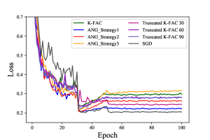
(a) Validation Loss vs. Epoch

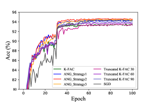
(b) Validation Accuracy vs. Epoch

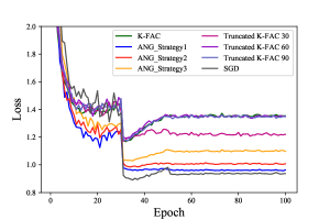
(c) Validation Loss vs. Epoch

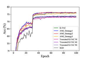
(d) Validation Accuracy vs. Epoch

Figure 1: Performance comparison among SGD, K-FAC, ANG and Truncated K-FAC on CIFAR-10 and CIFAR-100. (a), (b) show the accuracy and loss curves on CIFAR-10 respectively, and (c), (d) on CIFAR-100. In the legend, we name ANG with different strategies as ANG_strategy1, ANG_strategy2 and ANG_strategy3. Three curves of switching K-FAC to SGD at 30, 60 and 90 epoch are named as Truncated K-FAC 30, 60 and 90 respectively.

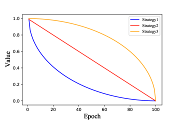
Figure 2: Three different strategies for $\lambda$, which controls the mixing ratio of second-order and first-order methods.

Then, we analyze the impact of different $\lambda$ parameter strategies on ANG performance, as shown in Fig. 2. Correspondingly, through the resultsin Fig. 1, we find that the more "concave" strategy 1 is closer to the first-order generalization performance on loss, and has the best suppression of overfitting. In terms of accuracy, strategy 1 also achieved the most stable and excellent performance in the both two data sets.

3.1.1 Part Two

In this part, we focus on analyzing the performance of IFANG. In order to solve the inverse problem in second-order optimization, we introduce a 1-rank natural gradient estimation method based on ANG. ANG adopted more extreme sampling strategy. In view of the convolution and full connection layer, by compressing of feature dimension to 1, it gets 1 rank activation layer and layer gradient subspace, and by adopting the technology of SMW method, the dimension of factorized matrix can be reduced to 1. Finally, The calculation of the inverse matrix is reduced to the inverse of a scalar. Due to further estimation, some curvature information is lost. IFANG delivers slightly less impressive but acceptable performance of accuracy and loss, as shown in Fig. 3. However, we counted the wall-clock time of different algorithms and found IFANG’s amazing advantage in speed. The detailed iteration times are exhibited in Table 1. Specifically, from the perspective of the time of each epoch, IFANG reduced by 23% compared with K-FAC. For a single iteration involving inversion, IFANG performed almost as well as SGD and was about 90% more efficient than K-FAC. As for ANG, it adds some extra steps to integrate the gradient compared to k-FAC, thus slightly increasing the time.

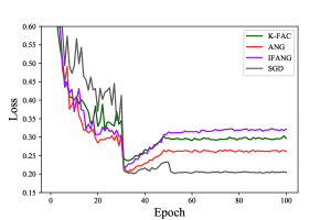
(a) Validation Loss vs. Epoch

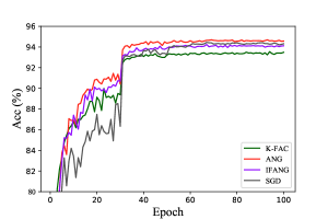
(b) Validation Accuracy vs. Epoch

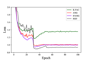
(c) Validation Loss vs. Epoch

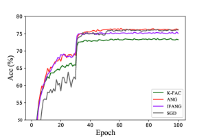
(d) Validation Accuracy vs. Epoch

Figure 3: Performance comparison among SGD, K-FAC, ANG and Truncated K-FAC on CIFAR-10 and CIFAR-100. (a), (b) show the accuracy and loss curves on CIFAR-10 respectively, and (c), (d) on CIFAR-100.

Table 1: Time consumptions of different methods

Algorithm	Time consumption per iteration($s$)	Time Gap	Time consumption per epoch($s$)	Time Gap
K-FAC	4.77	0%	56.34	0%
SGD	0.0144	-99.70%	32.72	-41.92%
ANG	4.855	+1.78%	56.48	+0.24%
IFANG	0.341	-92.85%	43.2	-23.32%

4 Conclusion

From the perspective of generalization performance, the proposed ANG provides a smooth and progressive regularization strategy, which enables the training to learn quickly in the early stage at a second-order speed and converge in the later stage at a first-order generalization performance, without any oscillation caused by mode collapse. In addition, to solve the problem of hard inverse in the second order, we further proposed a natural gradient algorithm IFANG without demand-inverse based on ANG. This algorithm is a more friendly alternative to different devices when the computing power is limited.

References

- He et al. [2016] Kaiming He, Xiangyu Zhang, Shaoqing Ren, and Jian Sun. Deep residual learning for image recognition. In Proceedings of the IEEE conference on computer vision and pattern recognition, pages 770–778, 2016.
- Ren et al. [2015] Shaoqing Ren, Kaiming He, Ross Girshick, and Jian Sun. Faster r-cnn: Towards real-time object detection with region proposal networks. In Advances in neural information processing systems, pages 91–99, 2015.
- Vaswani et al. [2017] Ashish Vaswani, Noam Shazeer, Niki Parmar, Jakob Uszkoreit, Llion Jones, Aidan N Gomez, Łukasz Kaiser, and Illia Polosukhin. Attention is all you need. In Advances in neural information processing systems, pages 5998–6008, 2017.
- Silver et al. [2016] David Silver, Aja Huang, Chris J Maddison, Arthur Guez, Laurent Sifre, George Van Den Driessche, Julian Schrittwieser, Ioannis Antonoglou, Veda Panneershelvam, Marc Lanctot, et al. Mastering the game of go with deep neural networks and tree search. nature, 529(7587):484–489, 2016.
- Goyal et al. [2017] Priya Goyal, Piotr Dollár, Ross Girshick, Pieter Noordhuis, Lukasz Wesolowski, Aapo Kyrola, Andrew Tulloch, Yangqing Jia, and Kaiming He. Accurate, large minibatch sgd: Training imagenet in 1 hour. arXiv preprint arXiv:1706.02677, 2017.
- Duchi et al. [2011] John Duchi, Elad Hazan, and Yoram Singer. Adaptive subgradient methods for online learning and stochastic optimization. Journal of machine learning research, 12(7), 2011.
- Zeiler [2012] Matthew D Zeiler. Adadelta: an adaptive learning rate method. arXiv preprint arXiv:1212.5701, 2012.
- Tieleman and Hinton [2012] Tijmen Tieleman and Geoffrey Hinton. Lecture 6.5-rmsprop: Divide the gradient by a running average of its recent magnitude. COURSERA: Neural networks for machine learning, 4(2):26–31, 2012.
- Kingma and Ba [2014] Diederik P Kingma and Jimmy Ba. Adam: A method for stochastic optimization. arXiv preprint arXiv:1412.6980, 2014.
- Arbel et al. [2019] Michael Arbel, Arthur Gretton, Wuchen Li, and Guido Montúfar. Kernelized wasserstein natural gradient. arXiv preprint arXiv:1910.09652, 2019.
- Amari [1998] Shun-Ichi Amari. Natural gradient works efficiently in learning. Neural computation, 10(2):251–276, 1998.
- Heskes [2000] Tom Heskes. On “natural” learning and pruning in multilayered perceptrons. Neural Computation, 12(4):881–901, 2000.
- Martens and Grosse [2015] James Martens and Roger Grosse. Optimizing neural networks with kronecker-factored approximate curvature. In International conference on machine learning, pages 2408–2417, 2015.
- Ollivier [2015] Yann Ollivier. Riemannian metrics for neural networks i: feedforward networks. Information and Inference: A Journal of the IMA, 4(2):108–153, 2015.
- Povey et al. [2014] Daniel Povey, Xiaohui Zhang, and Sanjeev Khudanpur. Parallel training of dnns with natural gradient and parameter averaging. arXiv preprint arXiv:1410.7455, 2014.
- Roux et al. [2007] Nicolas Roux, Pierre-Antoine Manzagol, and Yoshua Bengio. Topmoumoute online natural gradient algorithm. Advances in neural information processing systems, 20:849–856, 2007.
- Wilson et al. [2017] Ashia C Wilson, Rebecca Roelofs, Mitchell Stern, Nati Srebro, and Benjamin Recht. The marginal value of adaptive gradient methods in machine learning. In Advances in neural information processing systems, pages 4148–4158, 2017.
- Reddi et al. [2019] Sashank J Reddi, Satyen Kale, and Sanjiv Kumar. On the convergence of adam and beyond. arXiv preprint arXiv:1904.09237, 2019.
- Keskar and Socher [2017] Nitish Shirish Keskar and Richard Socher. Improving generalization performance by switching from adam to sgd. arXiv preprint arXiv:1712.07628, 2017.
- Anil et al. [2020] Rohan Anil, Vineet Gupta, Tomer Koren, Kevin Regan, and Yoram Singer. Second order optimization made practical, 2020.
- Osawa et al. [2019] Kazuki Osawa, Yohei Tsuji, Yuichiro Ueno, Akira Naruse, Rio Yokota, and Satoshi Matsuoka. Large-scale distributed second-order optimization using kronecker-factored approximate curvature for deep convolutional neural networks. In Proceedings of the IEEE Conference on Computer Vision and Pattern Recognition, pages 12359–12367, 2019.
- Zhang [2018] Zijun Zhang. Improved adam optimizer for deep neural networks. In 2018 IEEE/ACM 26th International Symposium on Quality of Service (IWQoS), pages 1–2. IEEE, 2018.
- Grosse and Martens [2016] Roger Grosse and James Martens. A kronecker-factored approximate fisher matrix for convolution layers. In International Conference on Machine Learning, pages 573–582, 2016.