Perturbed Runge-Kutta methods for mixed precision applications

Abstract

In this work we consider a mixed precision approach to accelerate the implemetation of multi-stage methods. We show that Runge–Kutta methods can be designed so that certain costly intermediate computations can be performed as a lower-precision computation without adversely impacting the accuracy of the overall solution. In particular, a properly designed Runge–Kutta method will damp out the errors committed in the initial stages. This is of particular interest when we consider implicit Runge–Kutta methods. In such cases, the implicit computation of the stage values can be considerably faster if the solution can be of lower precision (or, equivalently, have a lower tolerance). We provide a general theoretical additive framework for designing mixed precision Runge–Kutta methods, and use this framework to derive order conditions for such methods. Next, we show how using this approach allows us to leverage low precision computation of the implicit solver while retaining high precision in the overall method. We present the behavior of some mixed-precision implicit Runge–Kutta methods through numerical studies, and demonstrate how the numerical results match with the theoretical framework. This novel mixed-precision implicit Runge–Kutta framework opens the door to the design of many such methods.

1 Introduction

Consider the ordinary differential equation (ODE)

$$u_{t}=F(u).$$

Evolving this equation using a standard Runge Kutta approach we have the $s$-stage Runge–Kutta method

$$y^{(i)}=u^{n}+\Delta t\sum_{j=1}^{s}A_{ij}F(y^{(j)})$$

(1) $$u^{n+1}=u^{n}+\Delta t\sum_{j=1}^{s}b_{j}F(y^{(j)}),$$

where $A^{sxs}$ and $b^{1xs}$ are known as the Butcher coefficients of the method.

The computational cost of the function evaluations $F(y^{(j)})$ can be considerable, especially in cases where it necessitates an implicit solve. The use of mixed precision approach has been implemented for other numerical methods [1, 5] seems to be a promising approach. Lowering the precision on these computations, either by storing $F(y^{(j)})$ as a single precision variable rather than a double precision one, or by raising the tolerance of the implicit solver, can speed up the computation significantly. However, it generally reduces the precision of the overall numerical solution.

The aim of this paper is to create a framework for the design of Runge–Kutta methods that allow lower precision function evaluations for some of the stages, without impacting the overall precision of the solution. This acceleration of multi-stage methods using a mixed precision approach relies on a design that ensures that errors committed in the early stages may be damped out by the construction of the update in later stages.

The structure of this paper is as follows: in Section 2 we provide a numerical example of a mixed-precision formulation of the implicit midpoint rule, which motivates the need to study the effect of lower-precision computations of implicit function evaluations. In 3 we provide a general framework for analyzing mixed-precision Runge–Kutta methods by exploiting the additive Runge–Kutta method formulation. In this section we also present the order conditions that arise from this formulation and show how these are a relaxation of the general required order conditions. In Section 4 we show how the implicit midpoint rule can be written in this additive mixed-precision Runge–Kutta form, and develop methods in a specific class of implicit Runge–Kutta methods that exploit the formulation in Section 3.

2 Motivating example: mixed precision implementation of the implicit midpoint rule

First we consider the implicit midpoint rule defined as

(2) $$u^{n+1}=u^{n}+\Delta tF\left(\frac{u^{n}+u^{n+1}}{2}\right)$$

which is equivalently written in its Butcher form as:

(3a) $$y^{(1)} =u^{n}+\frac{\Delta t}{2}F\left(y^{(1)}\right)$$

(3b) $$u^{n+1} =u^{n}+\Delta tF\left(y^{(1)}\right)$$

The equivalence can be seen by noting that equation (3b) can be re-written as $u^{n+1}=2y^{(1)}-u^{n}$, and substituting $y^{(1)}=\frac{1}{2}(u^{n}+u^{n+1})$ into equation (3a).

In both equations (2) and (3a), we require an implicit solver in order to compute the update. Let’s consider the case that the implicit solver can only be satisfied up to some tolerance, $O(\epsilon)$, who’s output ${u_{\epsilon}}^{n+1}$ satisfies the modified equation

$${u_{\epsilon}}^{n+1}=u^{n}+\Delta tF^{\epsilon}\left(\frac{u^{n}+{u_{\epsilon}}^{n+1}}{2}\right)$$

exactly. We define the perturbation operator

(4) $$\tau(u)=\frac{F(u)-F^{\epsilon}(u)}{\epsilon}$$

so at any given time-step $u^{n+1}-{u_{\epsilon}}^{n+1}$ = $O(\epsilon\Delta t)$. Over the course of the solution, the local errors build-up to give an global error contribution of $O(\epsilon)$.

However, we can also formulate a method

(5a) $${y_{\epsilon}}^{(1)} =u^{n}+\frac{\Delta t}{2}F^{\epsilon}\left(y_{\epsilon}^{(1)}\right)$$

(5b) $$\hat{u}^{n+1} =u^{n}+\Delta tF\left(y_{\epsilon}^{(1)}\right)$$

where we use an inaccurate implicit solve in the first stage, and an accurate explicit evaluation in the second stage. We obtain $y_{\epsilon}^{(1)}=y^{(1)}+\Delta tO(\epsilon)$. The error, ${u}^{n+1}-\hat{u}^{n+1}$, between the full precision and mixed precision implementation over one time-step is now of order $O(\epsilon\Delta t^{2})$. This results in a global error contribution of $O(\epsilon\Delta t)$.

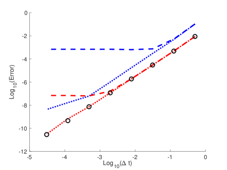
Figure 1: The implicit midpoint rule applied to the van der Pol system (6). The half-precision implementation ($\epsilon=O(10^{-4})$) is shown as a blue dashed line and the single-precision implementation $\epsilon=O(10^{-8})$ as a red dashed line. The mixed precision implementation with $\epsilon=O(10^{-4})$ is shown with a dotted blue line, and the mixed precision implementation with $\epsilon=O(10^{-8})$ is shown with a dotted red line. The double precision implementation is shown for reference with black circles.

To see how this works in practice, consider the van der Pol system

(6a) $$y_{1}^{\prime} = y_{2}$$

(6b) $$y_{2}^{\prime} = \;y_{2}\;(1-y_{1}^{2})-y_{1}$$

with initial conditions $y_{1}(0)=2$ and $y_{2}(0)=0$. We stepped this forward to a final time $T_{f}=1.0$. To emulate a mixed precision computation, we let $F^{\epsilon}$ in (5a) be the truncated output of $F$, where the truncation is performed to single precision ($\epsilon\approx 10^{-8}$) and half precision ($\epsilon\approx 10^{-4}$), while the explicit evaluation of $F$ in (5b) is performed in double precision. For comparison, we emulate a low precision version of (3), where we truncate all computations of $F$ in to the same low precision. Finally, we compute a full -precision version of (3), where all $F$ are computed to double precision and not truncated. (Note that his truncation approach is advocated in [7] to emulate low precision simulations.)

In Figure 1, we show the final time errors in the simulation using the various implementations. First, we look at the errors from a low-precision implementation (3) in which all the computations of $F$ are truncated to single precision (blue dashed line) or half precision (red dashed line). Clearly, for a sufficiently refined $\Delta t$, these errors look like $O(\epsilon)$. Next, we look at the errors from the mixed precision computation, given by Equation (5), has a value of $F^{\epsilon}$ that results from a single precision (blue dotted line) truncation or a half-precision truncation (red dotted line), and an explicit $F$ that is evaluated in full precision. These errors are clearly much better: they are convergent initially at second order, and the implementation with $\epsilon\approx 10^{-8}$ remains second order, and matches the full-precision implementation (black circles). However, the implementation using $\epsilon\approx 10^{-4}$ reduces to first order for a sufficiently small $\Delta t$. In the next section we construct a general framework that explains why this happens and allows us to construct higher order methods that work well in a mixed precision formulation.

3 A general framework for the analysis of mixed precision Runge–Kutta methods

We use the B-series analysis for additive Runge Kutta methods to develop consistency and perturbation conditions for the mixed precision Runge Kutta method of the form:

(7a) $$y^{(i)}=u^{n}+\Delta t\sum_{j=1}^{s}A_{ij}F(y^{(j)})+\Delta t\sum_{j=1}^{s}A^{\epsilon}_{ij}F^{\epsilon}(y^{(j)})$$

(7b) $$u^{n+1}=u^{n}+\Delta t\sum_{j=1}^{s}b_{j}F(y^{(j)})+\Delta t\sum_{j=1}^{s}b^{\epsilon}_{j}F^{\epsilon}(y^{(j)}).$$

Such methods have been extensively studied, including [3, 4, 12]

In [8] a perturbation approach to Runge–Kutta methods was proposed in order to increase the largest allowable time-step that preserved strong stability. Following a similar approach we note that the operator $F^{\epsilon}(y)$ is an approximation to $F(y)$ such that for any $y$ we require $F^{\epsilon}(y)-F(y)=O(\epsilon)$. This allows us to rewrite the scheme to evolve the operator $F$ and its perturbation $\tau$, defined in (4):

(8a) $$y^{(i)} =u^{n}+\Delta t\sum_{j=1}^{s}\tilde{A}_{ij}F(y^{(j)})+\epsilon\Delta t\sum_{j=1}^{s}A^{\epsilon}_{ij}\tau(y^{(j)})$$

(8b) $$u^{n+1} =u^{n}+\Delta t\sum_{j=1}^{s}\tilde{b}_{j}F(y^{(j)})+\epsilon\Delta t\sum_{j=1}^{s}b^{\epsilon}_{j}\tau(y^{(j)})$$

where $\tilde{A}_{ij}=A_{ij}+A^{\epsilon}_{ij}$ and $\tilde{b}=b_{j}+b^{\epsilon}_{j}$.

Analyzing the scheme in this form allows us to use an additive B-series representation to track the evolution of $F$ as well as its interaction with the perturbation function $\tau$. For example, a second order expansion is:

(9) $$u^{n+1} =\underbrace{u^{n}+\Delta t\tilde{b}eF(u^{n})+\Delta t^{2}\tilde{b}\tilde{c}F_{y}(u^{n})F(u^{n})}_{scheme}$$

$$+\underbrace{\epsilon\Delta t\left(b^{\epsilon}e\tau(u^{n})+\Delta t\left(b^{\epsilon}\tilde{c}\tau_{y}(u^{n})F(u^{n})+\tilde{b}c^{\epsilon}F_{y}(u^{n})\tau(u^{n})+\epsilon b^{\epsilon}c^{\epsilon}\tau_{y}(u^{n})\tau(u^{n})\right)\right)}_{perturbation}$$

$$+O(\Delta t^{3}).$$

This expansion shows two sources of error: those of the scheme and those of the perturbation, thus the error at one time-step can be written as the sum of the approximation error of the scheme, $E_{sch}$, and the perturbation error, $E_{per}.$ This leads to two sets of conditions under which a perturbed scheme has an error

$$E=E_{sch}+E_{per}=O(\Delta t^{p+1})+O(\epsilon\Delta t^{m+1})$$

at each time-step. A method with these errors will have a global error of the form

$$Error=O(\Delta t^{p})+O(\epsilon\Delta t^{m}).$$

We can easily extend (9) to higher order. The fourth order expansion related to the consistency of the scheme has following terms:

$$\begin{array}[]{lll}\hline\cr\mbox{Terms involving $\Delta t$}&\mbox{Terms involving $F$ }&\mbox{scheme}\\ &&\mbox{coefficients}\\ \hline\cr&&\\ \Delta t&F(u^{n})&\tilde{b}e\\ \Delta t^{2}&F_{y}(u^{n})F(u^{n})&\tilde{b}\tilde{c}\\ \Delta t^{3}&F_{y}(u^{n})F_{y}(u^{n})F(u^{n})&\tilde{b}\tilde{A}\tilde{c}\\ \Delta t^{3}&F_{yy}(u^{n})(F(u^{n}),F(u^{n}))&\tilde{b}(\tilde{c}\cdot\tilde{c})\\ \Delta t^{4}&F_{y}(u^{n})F_{y}(u^{n})F_{y}(u^{n})F(u^{n})&\tilde{b}\tilde{A}\tilde{A}\tilde{c}\\ \Delta t^{4}&F_{y}(u^{n})F_{yy}(u^{n})(F(u^{n}),F(u^{n}))&\tilde{b}\tilde{A}(\tilde{c}\cdot\tilde{c})\\ \Delta t^{4}&F_{yy}(u^{n})(F_{y}(u^{n})F(u^{n}),F(u^{n}))&\tilde{b}(\tilde{A}\tilde{c}\cdot\tilde{c})\\ \Delta t^{4}&F_{yyy}(u^{n})(F(u^{n}),F(u^{n}),F(u^{n}))&\tilde{b}(\tilde{c}\cdot\tilde{c}\cdot\tilde{c}).\end{array}$$

Expanding the terms related to the perturbation error to third order in $\Delta t$ and third order in $\epsilon$ we obtain:

$$\begin{array}[]{lll}\hline\cr\mbox{Terms involving }&\mbox{Terms involving }&\mbox{scheme}\\ \mbox{ $\epsilon$ and $\Delta t$}&\mbox{ $F$ and $\tau$}&\mbox{coefficients}\\ \hline\cr&&\\ \epsilon\Delta t&\tau(u^{n})&b^{\epsilon}e\\ \epsilon\Delta t^{2}&\tau_{y}(u^{n})F(u^{n})&b^{\epsilon}\tilde{c}\\ \epsilon\Delta t^{2}&F_{y}(u^{n})\tau(u^{n})&\tilde{b}c^{\epsilon}\\ \epsilon^{2}\Delta t^{2}&\tau_{y}(u^{n})\tau(u^{n})&b^{\epsilon}c^{\epsilon}\\ \epsilon\Delta t^{3}&\tau_{y}(u^{n})F_{y}(u^{n})\tau(u^{n})&b^{\epsilon}\tilde{A}\tilde{c}\\ \epsilon\Delta t^{3}&F_{y}(u^{n})\tau_{y}(u^{n})F(u^{n})&\tilde{b}A^{\epsilon}\tilde{c}\\ \epsilon\Delta t^{3}&F_{y}(u^{n})F_{y}(u^{n})\tau(u^{n})&\tilde{b}\tilde{A}c^{\epsilon}\\ \epsilon\Delta t^{3}&\tau_{yy}(u^{n})(F(u^{n}),F(u^{n}))&b^{\epsilon}(\tilde{c}\cdot\tilde{c})\\ \epsilon\Delta t^{3}&F_{yy}(u^{n})(F(u^{n}),\tau(u^{n}))&\tilde{b}(\tilde{c}\cdot c^{\epsilon})\\ \epsilon^{2}\Delta t^{3}&\tau_{y}(u^{n})\tau_{y}(u^{n})F(u^{n})&b^{\epsilon}A^{\epsilon}\tilde{c}\\ \epsilon^{2}\Delta t^{3}&\tau_{y}(u^{n})F(u^{n})\tau(u^{n})&b^{\epsilon}\tilde{A}c^{\epsilon}\\ \epsilon^{2}\Delta t^{3}&F_{y}(u^{n})\tau_{y}(u^{n})\tau(u^{n})&\tilde{b}A^{\epsilon}c^{\epsilon}\\ \epsilon^{2}\Delta t^{3}&\tau_{yy}(u^{n})(\tau(u^{n}),F(u^{n}))&b^{\epsilon}(c^{\epsilon}\cdot\tilde{c})\\ \epsilon^{3}\Delta t^{3}&\tau_{y}(u^{n})\tau_{y}(u^{n})\tau(u^{n})&b^{\epsilon}A^{\epsilon}c^{\epsilon}\\ \epsilon^{3}\Delta t^{3}&\tau_{yy}(u^{n})(\tau(u^{n}),\tau(u^{n}))&b^{\epsilon}(c^{\epsilon}\cdot c^{\epsilon})\\ \hline\cr\end{array}$$

From these terms, the consistency conditions for the scheme and the perturbation conditions can be easily defined, and are given in the next section. We consider two possible scenarios: In the standard scenario, we assume that both $F$ and $F^{\epsilon}$ are well-behaved functions, and all of their derivatives exist and are bounded. In this case, for the perturbation terms in the table above to be zeroed out, we simply impose the condition that the corresponding coefficient are zero. In the mixed precision scenario which motivated this formulation, we consider that $\tau$ comes from a precision error that is defined by ”chopping” the values at the desired precision. In this case, $F^{\epsilon}=Chop(F)$, so that the operator $F^{\epsilon}$ is bounded but not Lipshitz continuous, and so $\tau_{y}=\frac{F_{y}-F^{\epsilon}_{y}}{\epsilon}$ is also not Lipshitz continuous, i.e $\frac{\partial^{(k)}\tau}{\partial y^{(k)}}$ does not exist. In this case, we must ensure that all terms containing $\tau_{y}$ are multiplied by zero coefficients in the expansion, without assuming cancellation errors. In other words, we requires more stringent conditions to ensure that terms of the form $\tau_{y},\tau_{yy}$ etc. do not appear in the final stage. This means that whereas when $\tau$ is a well-behaved function, it is sufficient to require that $b^{\epsilon}c=0$, instead we must require that not only the sum is zero, but every term: $b^{\epsilon}_{j}c_{j}=0$. We denote conditions of this form with absolute values (e.g. $|b^{\epsilon}||c|=0$). These stringent conditions apply to each coefficient matrix/vector which appears in conditions corresponding to derivatives of tau. These conditions are presented in the next subsection.

3.1 Consistency Conditions and Perturbation Conditions

The consistency and perturbation conditions can be derived from the additive B-series analysis of the scheme defined by equations (8a-8b). Terms that involve only $F$ yield the classical consistency conditions of the unperturbed scheme. The cross terms are the perturbation errors. A perturbed Runge-Kutta method is of consistency order $p$ if the following conditions are satisfied:

(10) $$\begin{array}[]{ll}\text{For }p\geq 1:&\;\;\;\;\tilde{b}e=1\\ \text{For }p\geq 2:&\;\;\;\;\tilde{b}\tilde{c}=\frac{1}{2}\\ \text{For }p\geq 3:&\;\;\;\;\tilde{b}(\tilde{c}\cdot\tilde{c})=\frac{1}{3}\;\;\;\mbox{and}\;\;\;\tilde{b}\tilde{A}\tilde{c}=\frac{1}{6}\\ \text{For }p\geq 4:&\;\;\;\;\tilde{b}(\tilde{c}\cdot\tilde{c}\cdot\tilde{c})=\frac{1}{4},\;\;\tilde{b}(\tilde{A}\tilde{c}\cdot\tilde{c})=\frac{1}{8},\;\;\;\;\tilde{b}\tilde{A}(\tilde{c}\cdot\tilde{c})=\frac{1}{12},\;\;\mbox{and}\;\;\;\tilde{b}\tilde{A}\tilde{A}\tilde{c}=\frac{1}{24}.\end{array}$$

The perturbation errors are determined by both $\Delta t$ and $\epsilon$. For a scheme to achieve order $O(\epsilon\Delta t^{m+1})$ we require :

• For $m\geq 1$ we require

  (11a) $$\mbox{for}\;\;n\geq 1:\;\;\;\; b^{\epsilon}e=0$$

• For $m\geq 2$ we require

  (11b) $$\mbox{for}\;\;n\geq 1:\;\;\; |b^{\epsilon}||\tilde{c}|=0\;\;\mbox{and}\;\;\tilde{b}c^{\epsilon}=0$$

  (11c) $$\mbox{for}\;\;n\geq 2:\;\;\; |b^{\epsilon}||c^{\epsilon}|=0$$

• For $m\geq 3$ we require

  (11d) $$\mbox{for}\;\;n\geq 1:\;\;\;\; |b^{\epsilon}||\tilde{A}||\tilde{c}|=0,\;\;|\tilde{b}||A^{\epsilon}||\tilde{c}|=0,\;\;\tilde{b}\tilde{A}c^{\epsilon}=0,$$

  $$|b^{\epsilon}|\left|(\tilde{c}\cdot\tilde{c})\right|=0,\;\;\;\;\tilde{b}(\tilde{c}\cdot c^{\epsilon})=0,$$

  (11e) $$\mbox{for}\;\;n\geq 2:\;\;\;\; |b^{\epsilon}||A^{\epsilon}||\tilde{c}|=0,\;\;|b^{\epsilon}||\tilde{A}||c^{\epsilon}|=0,\;\;|\tilde{b}||A^{\epsilon}||c^{\epsilon}|=0,$$

  $$|b^{\epsilon}|\left|(c^{\epsilon}\cdot\tilde{c})\right|=0,\;\;\tilde{b}(c^{\epsilon}\cdot c^{\epsilon})=0,$$

  (11f) $$\mbox{for}\;\;n\geq 3:\;\;\;\; |b^{\epsilon}||A^{\epsilon}||c^{\epsilon}|=0,\;\;|b^{\epsilon}|\left|(c^{\epsilon}\cdot c^{\epsilon})\right|=0.$$

Note that the coefficients that are not attached to a derivative (see table above), do not require the absolute value.

In the Subsection 3.2 we will show how these conditions can explain the behavior of the mixed-precision implementation of the implicit midpoint rule. In Section 4 we will use these conditions to derive mixed-precision methods.

3.1.1 Perturbation conditions when $\tau$ is well behaved

If $\tau$ is a well-behaved function, we can assume that terms with similar terms will cancel. In this case, the perturbation conditions simplify. For a scheme to achieve order $O(\epsilon\Delta t^{m+1})$ we require:

• For $m\geq 1$ we require

  (12a) $$\mbox{for}\;\;n\geq 1:\;\;\;\; b^{\epsilon}e=0$$

• For $m\geq 2$ we require

  (12b) $$\mbox{for}\;\;n\geq 1:\;\;\; b^{\epsilon}\tilde{c}=0\;\;\mbox{and}\;\;\tilde{b}c^{\epsilon}=0$$

  (12c) $$\mbox{for}\;\;n\geq 2:\;\;\; b^{\epsilon}c^{\epsilon}=0$$

• For $m\geq 3$ we require

  (12d) $$\mbox{for}\;\;n\geq 1:\;\;\;\; b^{\epsilon}\tilde{A}\tilde{c}=0,\;\;\tilde{b}A^{\epsilon}\tilde{c}=0,\;\;\tilde{b}\tilde{A}c^{\epsilon}=0,$$

  $$b^{\epsilon}(\tilde{c}\cdot\tilde{c})=0,\;\;\;\;\tilde{b}(\tilde{c}\cdot c^{\epsilon})=0,$$

  (12e) $$\mbox{for}\;\;n\geq 2:\;\;\;\; b^{\epsilon}A^{\epsilon}\tilde{c}=0,\;\;b^{\epsilon}\tilde{A}c^{\epsilon}=0,\;\;\tilde{b}A^{\epsilon}c^{\epsilon}=0,$$

  $$b^{\epsilon}(c^{\epsilon}\cdot\tilde{c})=0,\;\;\tilde{b}(c^{\epsilon}\cdot c^{\epsilon})=0,$$

  (12f) $$\mbox{for}\;\;n\geq 3:\;\;\;\; b^{\epsilon}A^{\epsilon}c^{\epsilon}=0,\;\;b^{\epsilon}(c^{\epsilon}\cdot c^{\epsilon})=0.$$

3.2 Understanding the mixed precision implicit midpoint rule using the additive framework

Returning to the implicit midpoint rule example in Section 2, we can use the framework developed above to study the numerical behavior of the different implementations of the implicit midpoint rule. First, we consider the high precision form (3):

$$y^{(1)} =u^{n}+\frac{\Delta t}{2}F\left(y^{(1)}\right)$$

$$u^{n+1} =u^{n}+\Delta tF\left(y^{(1)}\right)$$

and note that it is exactly equivalent to (2). The low precision form of (3) and (2) is

(14a) $$y^{(1)} =u^{n}+\frac{\Delta t}{2}{F^{\epsilon}}\left(y^{(1)}\right)$$

(14b) $$u^{n+1} =u^{n}+\Delta tF^{\epsilon}\left(y^{(1)}\right)$$

while the mixed precision form is

(15a) $$y^{(1)} =u^{n}+\frac{\Delta t}{2}F^{\epsilon}\left(y^{(1)}\right)$$

(15b) $$u^{n+1} =u^{n}+\Delta tF\left(y^{(1)}\right).$$

Now let’s look at the coefficients of each of these schemes. The full-precision method (3) has coefficients:

$$\hskip 14.45377ptb=\left(\begin{array}[]{l}1\\ 0\\ \end{array}\right),\hskip 14.45377ptc=\left(\begin{array}[]{l}\frac{1}{2}\\ 1\\ \end{array}\right)\hskip 14.45377ptb^{\epsilon}=\left(\begin{array}[]{l}0\\ 0\\ \end{array}\right),\hskip 14.45377ptc^{\epsilon}=\left(\begin{array}[]{l}0\\ 0\\ \end{array}\right)$$

which satisfy the order conditions

$$\tilde{b}e=be+b^{\epsilon}e=1,\;\;\;\;\tilde{b}\tilde{c}=bc+bc^{\epsilon}+b^{\epsilon}c+b^{\epsilon}c^{\epsilon}=\frac{1}{2}.$$

The errors from the reduced precision operator are all zero:

$$b^{\epsilon}e=0,\;\;\;\;bc^{\epsilon}=b^{\epsilon}c=b^{\epsilon}c^{\epsilon}=0,$$

so that, as expected, there is no low precision contribution. This high precision method will produce second order global errors: $Error=O(\Delta t^{2})$.

Next, we look at the low-precision method (14)

$$b=\left(\begin{array}[]{l}0\\ 0\\ \end{array}\right),\hskip 14.45377ptc=\left(\begin{array}[]{l}0\\ 0\\ \end{array}\right),\hskip 14.45377ptb^{\epsilon}=\left(\begin{array}[]{l}1\\ 0\\ \end{array}\right),\hskip 14.45377ptc^{\epsilon}=\left(\begin{array}[]{l}\frac{1}{2}\\ 1\\ \end{array}\right).$$

Once again the $O(\Delta t^{2})$ consistency conditions are satisfied

$$\tilde{b}e=be+b^{\epsilon}e=1,\;\;\;\;\tilde{b}\tilde{c}=bc+bc^{\epsilon}+b^{\epsilon}c+b^{\epsilon}c^{\epsilon}=\frac{1}{2}.$$

However, the errors introduced by the reduced precision operator are given by the perturbation condition

$$b^{\epsilon}e=1,$$

so that at each time-step we have a perturbation error of the form

$$E_{per}=\epsilon\Delta tb^{\epsilon}e\tau(u^{n})=\Delta tO(\epsilon).$$

Putting this together, we expect to see errors of the form

$$E=O(\Delta t^{3})+O(\Delta t\epsilon)$$

at each time-step, and an overall error of

$$Error=O(\Delta t^{2})+O(\epsilon).$$

This explains the reduced accuracy we see in Figure 1, where initially the errors of $O(\Delta t^{2})$ dominate, but as $\Delta t$ gets small enough, the $O(\epsilon)$ terms dominate.

Finally, we look at the mixed-precision method (15)

$$b=\left(\begin{array}[]{l}1\\ 0\\ \end{array}\right),\hskip 14.45377ptc=\left(\begin{array}[]{l}0\\ 1\\ \end{array}\right),\hskip 14.45377ptb^{\epsilon}=\left(\begin{array}[]{l}0\\ 0\\ \end{array}\right),\hskip 14.45377ptc^{\epsilon}=\left(\begin{array}[]{l}\frac{1}{2}\\ 0\\ \end{array}\right).$$

We observe that, as before, the $O(\Delta t^{2})$ consistency conditions are satisfied

$$\tilde{b}e=be+b^{\epsilon}e=1,\;\;\;\;\tilde{b}\tilde{c}=bc+bc^{\epsilon}+b^{\epsilon}c+b^{\epsilon}c^{\epsilon}=0+\frac{1}{2}+0+0=\frac{1}{2},$$

so that $E_{sch}=\Delta t^{3}$. The perturbation errors from the reduced precision operator are

$$b^{\epsilon}e=0,\;\;\;\;bc^{\epsilon}=\frac{1}{2},\;\;b^{\epsilon}c=0,\;\;b^{\epsilon}c^{\epsilon}=0,$$

so that at each step we will see perturbation errors of the form

$$E_{per}=\epsilon\;\Delta t^{2}bc^{\epsilon}\;F^{\prime}(u^{n})\tau(u^{n})=\frac{1}{2}\;\epsilon\Delta t^{2}\;F^{\prime}(u^{n})\;\tau(u^{n})=O(\epsilon\Delta t^{2}).$$

Putting this together, we have a one-step error

$$E=E_{sch}+E_{per}=O(\Delta t^{3})+O(\epsilon\Delta t^{2}),$$

so that over the course of the simulation we expect to see error of the form

$$Error=O(\Delta t^{2})+O(\epsilon\Delta t),$$

so that we expect to see second order results as long as $\epsilon\Delta t$ is small enough, and after that will produce results that look like $\epsilon\Delta t$. This explains the excellent convergence we observe in Figure 1.

4 Efficient mixed-precision Runge–Kutta methods

In this section we exploit the framework in Section 3 to develop a mixed precision approach to Runge–Kutta methods. We first show how we can add correction steps into a naive implementation of a mixed-precision methods to raise the perturbation order of the method, as computed by the conditions in Section 3.1. Next we use the order and perturbation conditions to develop novel efficient methods that have high consistency order and high perturbation order using an appropriate optimization code similar to those described in [9].

4.1 Mixed precision implementation and corrections to known Runge–Kutta methods

In this section, we show that often, low-precision computation of the implicit function yields naive mixed-precision methods that have perturbation errors that may degrade the accuracy of the solution for sufficiently small $\Delta t$. It is possible to correct this by adding high order explicit steps; this approach yields methods that can be shown to satisfy both the consistency (10) and perturbation conditions (11).

4.1.1 Implicit Midpoint rule with correction

The mixed precision implicit midpoint rule we described above (15)

$$y^{(1)} =u^{n}+\frac{\Delta t}{2}F^{\epsilon}\left(y^{(1)}\right)$$

$$u^{n+1} =u^{n}+\Delta tF\left(y^{(1)}\right).$$

has global error

$$Error=O(\Delta t^{2})+O(\epsilon\Delta t)$$

so that it gives second order ($O(\Delta t^{2})$) results as long as $\epsilon\Delta t$ is small enough; once $\Delta t$ gets small compared to $\epsilon$ we observe degraded convergence. To eliminate this error, we wish to modify the method (15) so that the $O(\epsilon\Delta t^{2})$ term in the expansion (9) is set to zero. The framework above suggests how this can be done. To improve the order of convergence, when $\Delta t$ is small we add correction terms into the mixed-precision method:

(16a) $$y^{(1)}_{[0]} =u^{n}+\frac{1}{2}\Delta tF^{\epsilon}(y^{(1)}_{[0]})$$

(16b) $$y^{(1)}_{[k]} =u^{n}+\frac{1}{2}\Delta tF(y^{(1)}_{[k-1]})\;\;\;\mbox{for}\;\;k=1,...,p-1$$

(16c) $$u^{n+1} =u^{n}+\Delta tF\left(y^{(1)}_{[p-1]})\right).$$

so that

$$A=\left(\begin{array}[]{ll}0&0\\ \frac{1}{2}&0\\ \end{array}\right),\;\;\;c=\left(\begin{array}[]{l}0\\ \frac{1}{2}\\ \end{array}\right),\;\;\;b=\left(\begin{array}[]{l}0\\ 1\\ \end{array}\right),\;\;\;$$

$$A^{\epsilon}=\left(\begin{array}[]{lll}\frac{1}{2}&0\\ 0&0\\ \end{array}\right),\;\;\;c^{\epsilon}=\left(\begin{array}[]{l}\frac{1}{2}\\ 0\\ \end{array}\right),\;\;\;b^{\epsilon}=\left(\begin{array}[]{l}0\\ 0\\ \end{array}\right),\;\;\;$$

$$\tilde{A}=A+A^{\epsilon}=\left(\begin{array}[]{lll}\frac{1}{2}&0\\ \frac{1}{2}&0\\ \end{array}\right),\;\;\;\tilde{c}=c+c^{\epsilon}=\left(\begin{array}[]{l}\frac{1}{2}\\ \frac{1}{2}\\ \end{array}\right),\;\;\;\tilde{b}=b+b^{\epsilon}=\left(\begin{array}[]{l}0\\ 1\\ \end{array}\right).\;\;\;$$

We observe that to zero out the $O(\epsilon\Delta t^{2})$ term we require

$$b^{\epsilon}\tilde{c}=0,\;\;\tilde{b}c^{\epsilon}=0.$$

The method (16) satisfies these equations, and so we obtain global error:

$$Error=O(\Delta t^{2})+O(\epsilon\Delta t^{2}).$$

Note that this approach to reduce precision errors is reminiscent of that in [10]; the framework we developed allows us to understand this correction approach as a new method.

Numerical Results: In the following we demonstrate how this method performs in practice. As before, we use the van der Pol system, Equation (6) with $a=1$ and initial conditions $y_{1}(0)=2$ and $y_{2}(0)=0$. We stepped this forward using the implicit midpoint rule (16) to a final time $T_{f}=1.0$. We show how using a mixed precision implementation and then a correction step (16b) improves the error. In Figure 2 we show the results for $\epsilon=O(1)$ (zero precision, left), $\epsilon=O(10^{-4})$ (half precision), and $\epsilon=O(10^{-8})$ (single precision, right). The low precision (14) is shown in a dashed line, the mixed precision method (16) with no correction ($p=1$) in a dotted line, and the mixed precision method (16) with one correction $(p=2)$ in a dash-dot line. The reference solution computed in double precision is shown in black circle markers.

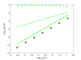
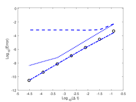
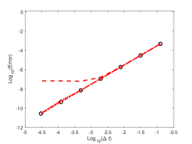
Figure 2: The implicit midpoint rule applied to the van der Pol system (6) with correction steps. Left: Zero precision $\epsilon=O(1)$, Middle: half precision $\epsilon=O(10^{-4})$, Right: single precision $\epsilon=O(10^{-8})$.

Figure 2 shows that each progressive correction, which involves explicit computation of the function, produces a more accurate method. Looking at the perturbation conditions, we showed in Section 3.2 that the low precision method (14) has errors $Error_{LP}=O(\Delta t^{2})+O(\epsilon).$ As expected, dashed line solutions shown in Figure 2 all have flat line errors at the level of their respective $\epsilon$ values.

The mixed precision method (16) with $p=1$ (this is the same method give by Equation (15)), has errors $Error_{p=1}=O(\Delta t^{2})+O(\epsilon\Delta t),$ which is reflected in the fact that the dotted line solutions for the zero precision case in Figure 2 has slope $\sigma=1$. For the half precision case the dotted line solution starts off with a slope $\sigma=2$, but once the time-step gets sufficiently small we see the line changes and now has slope $\sigma=1$: this shows clearly that once $\Delta t$ is small enough compared to $\epsilon$, the $O(\epsilon\Delta t)$ term dominates and we see first order convergence. For the single precision, we don’t observe this phenomenon in this example because $\Delta t$ is not small enough compared to $\epsilon$.

Finally, the mixed precision method with one correction step (Equation (16) with $p=2$ ) has errors $Error_{p=2}=O(\Delta t^{2})+O(\epsilon\Delta t^{2}).$ For the half and single precision, two corrections steps produce a second order solution, and this line has $\sigma=2$. The order of the same accuracy as a complete computation in double precision (shown in black circles). This would be worth-while in all cases where two explicit steps take much less computational time than the savings realized from replacing a double-precision implicit solve with one that has single or half precision. The case of zero precision, $\epsilon=O(1)$, has a larger error, but the correction step clearly gives an error with slope $\sigma=2$.

4.1.2 A mixed precision implementation of a two stage third order SDIRK

We take the two stage third order singly diagonally implicit method [2]

(17a) $$y^{(1)} = u^{n}+\gamma\Delta tF(y^{(1)})$$

(17b) $$y^{(2)} = u^{n}+\left(1-2\gamma\right)\Delta tF(y^{(1)})+\gamma\Delta tF(y^{(2)})$$

(17c) $$u^{n+1} = u^{n}+\frac{1}{2}\Delta tF(y^{(1)})+\frac{1}{2}\Delta tF(y^{(2)})$$

with $\gamma=\frac{\sqrt{3}+3}{6}$. A low-precision implementation is given by

(18a) $$y^{(1)} = u^{n}+\gamma\Delta tF^{\epsilon}(y^{(1)})$$

(18b) $$y^{(2)} = u^{n}+\left(1-2\gamma\right)\Delta tF^{\epsilon}(y^{(1)})+\gamma\Delta tF^{\epsilon}(y^{(2)})$$

(18c) $$u^{n+1} = u^{n}+\frac{1}{2}\Delta tF(y^{(1)})+\frac{1}{2}\Delta tF^{\epsilon}(y^{(2)}).$$

Using a low-precision computation only of the implicit function yields the mixed-precision method:

(19a) $$y^{(1)} = u^{n}+\gamma\Delta tF^{\epsilon}(y^{(1)})$$

(19b) $$y^{(2)} = u^{n}+\left(1-2\gamma\right)\Delta tF(y^{(1)})+\gamma\Delta tF^{\epsilon}(y^{(2)})$$

(19c) $$u^{n+1} = u^{n}+\frac{1}{2}\Delta tF(y^{(1)})+\frac{1}{2}\Delta tF(y^{(2)}).$$

The consistency conditions are satisfied to order three. The highest order non-zero perturbation term is $\tilde{b}c^{\epsilon}=\gamma$ so we have a perturbation error $E_{per}=O(\Delta t^{2}\epsilon)$ at each time step, or a global error

$$Error=O(\Delta t^{3})+O(\epsilon\Delta t).$$

When $\Delta t^{2}<\epsilon$, the perturbation error will dominate. In this case, we can correct the method by adding explicit stages:

(20a) $$y_{[0]}^{(1)} = u^{n}+\gamma\Delta tF^{\epsilon}(y^{(1)}_{[0]})$$

(20b) $$y_{[k]}^{(1)} = u^{n}+\gamma\Delta tF(y^{(1)}_{[k-1]})\;\;\;\mbox{for}\;\;k=1,...,p-1$$

(20c) $$y_{[0]}^{(2)} = u^{n}+(1-2\gamma)\Delta tF(y^{(1)}_{[p-1]})+\gamma\Delta tF(y^{(2)}_{[0]})$$

(20d) $$y_{[k]}^{(2)} = u^{n}+(1-2\gamma)\Delta tF(y^{(1)}_{[p-1]})+\gamma\Delta tF(y^{(2)}_{[k-1]})\;\;\;\mbox{for}\;\;k=1,...,p-1$$

(20e) $$u^{n+1} = u^{n}+\frac{1}{2}\Delta tF(y^{(1)}_{[p-1]}))+\frac{1}{2}\Delta tF(y^{(2)}_{[p-1]})).$$

This corrected method with $p=3$ has coefficients:

$$A=\left(\begin{array}[]{cccccc}0&0&0&0&0&0\\ \gamma&0&0&0&0&0\\ 0&\gamma&0&0&0&0\\ 0&0&(1-2\gamma)&0&0&0\\ 0&0&(1-2\gamma)&\gamma&0&0\\ 0&0&(1-2\gamma)&0&\gamma&0\\ \end{array}\right),\;\;\;\;A^{\epsilon}=\left(\begin{array}[]{cccccc}\gamma&0&0&0&0&0\\ 0&0&0&0&0&0\\ 0&0&0&0&0&0\\ 0&0&0&\gamma&0&0\\ 0&0&0&0&0&0\\ 0&0&0&0&0&0\\ \end{array}\right)$$

$$b=\left(\begin{array}[]{cccccc}0&0&\frac{1}{2}&0&0&\frac{1}{2}\\ \end{array}\right),\;\;\;\;b^{\epsilon}=\left(\begin{array}[]{cccccc}0&0&0&0&0&0\\ \end{array}\right).\;$$

The order conditions are, as before, satisfied to third order, and the perturbation terms contribute to the errors terms of the form $O(\epsilon\Delta t^{4})$, so the overall global error from the method with three corrections for each implicit solve is

$$Error_{p=3}=O(\Delta t^{3})+O(\epsilon\Delta t^{3}).$$

Numerical Results: To demonstrate the performance of this method in practice, we apply its various implementations to the van der Pol system, Equation (6), with $a=1$ and initial conditions $y_{1}(0)=2$ and $y_{2}(0)=0$. We step this forward to a final time $T_{f}=1.0$, using low precision, mixed precision, and mixed precision with successive corrections.

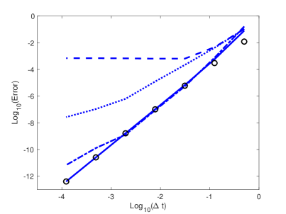
Figure 3: The SDIRK method with successive corrections applied to the van der Pol system (6). The half-precision implementation (18)) shown as a dashed line. The mixed precision implementation (19)) with $\epsilon=O(10^{-4})$ is shown with a dotted line. The mixed precision implementation (20) with $\epsilon=O(10^{-4})$ and one ($p=2$) correction steps is shown with dash-dot, and with two ($p=3$) correction steps with a solid line. The double precision implementation of (17) is shown for reference with black dots.

In Figure 3 we show the half-precision results of the various implementations of the SDIRK method. First, we use a half-precision implementation of the SDIRK method, as given in Equation (18)) with $\epsilon=O(10^{-4})$. The errors resulting from this implementation are shown by a dashed line. This line is horizontal at the level of $O(\epsilon)$, as expected from the error given by this implementation: $Error_{LP}=O(\Delta t^{3})+O(\epsilon).$ Using the naive mixed precision implementation (20) we expect an error of $Error_{p=1}=O(\Delta t^{3})+O(\epsilon\Delta t).$ In Figure 3, the dotted line shows that error initially has slope $\sigma=2$: this happens when $\epsilon$ is small compared to $\Delta t$ and so the $O(\epsilon\Delta t)$ looks like $O(\Delta t^{2})$. However, as $\Delta t$ gets smaller, we see the error line become first order. Adding one correction step to the mixed precision implementation (20), we obtain an error shown as the dash-dot line, which initially looks third order (slope $\sigma=3$) but then, as $\Delta t$ becomes small compared to $\epsilon$, begins to look like it is second order (slope $\sigma=3$). This matches the expected order $Error_{p=2}=O(\Delta t^{3})+O(\epsilon\Delta t^{2}).$ Finally, when we add two correction steps to the mixed precision implementation, the error (shown as a solid line) has slope $\sigma=3$, as expected from the predicted order $Error_{p=3}=O(\Delta t^{3})+O(\epsilon\Delta t^{3}).$ This solution matches the double precision reference solution shown in black circle markers.

4.1.3 Mixed precision implementation of a two stage L-stable scheme

Consider the L-stable fully implicit Lobatto IIIC scheme [11]:

(21a) $$y^{(1)} = u^{n}+\frac{1}{2}\Delta tF(y^{(1)})-\frac{1}{2}\Delta tF(y^{(2)})$$

(21b) $$y^{(2)} = u^{n}+\frac{1}{2}\Delta tF(y^{(1)})+\frac{1}{2}\Delta tF(y^{(2)})$$

(21c) $$u^{n+1} = y^{(2)}.$$

A naive mixed precision implementation of this method is given by:

(22a) $$y^{(1)} = u^{n}+\frac{1}{2}\Delta tF^{\epsilon}(y^{(1)})-\frac{1}{2}\Delta tF^{\epsilon}(y^{(2)})$$

(22b) $$y^{(2)} = u^{n}+\frac{1}{2}\Delta tF^{\epsilon}(y^{(1)})+\frac{1}{2}\Delta tF^{\epsilon}(y^{(2)})$$

(22c) $$u^{n+1} = u^{n}+\frac{1}{2}\Delta tF(y^{(1)})+\frac{1}{2}\Delta tF(y^{(2)})$$

This implementation has Butcher coefficients

$$A^{\epsilon}=\left(\begin{array}[]{rr}\frac{1}{2}&-\frac{1}{2}\\ \frac{1}{2}&\frac{1}{2}\\ \end{array}\right),\;\;\;\;A=\left(\begin{array}[]{rr}0&0\\ 0&0\\ \end{array}\right),$$

$$b^{\epsilon}=\left(\begin{array}[]{ll}0&0\end{array}\right),\;\;\;\;b=\left(\begin{array}[]{lll}\frac{1}{2}&\frac{1}{2}\end{array}\right).$$

The error coming from this implementation is, according to the analysis in Section 3,

$$Error=O(\Delta t^{2})+O(\epsilon\Delta t).$$

A corrected mixed precision implementation is given by

(23a) $$y^{(1)}_{[0]} = u^{n}+\frac{1}{2}\Delta tF^{\epsilon}(y^{(1)})-\frac{1}{2}\Delta tF^{\epsilon}(y^{(2)})$$

(23b) $$y^{(2)}_{[0]} = u^{n}+\frac{1}{2}\Delta tF^{\epsilon}(y^{(1)})+\frac{1}{2}\Delta tF^{\epsilon}(y^{(2)})$$

(23c) $$y^{(1)}_{[1]} = u^{n}+\frac{1}{2}\Delta tF(y^{(1)}_{[0]})-\frac{1}{2}\Delta tF(y^{(2)}_{[0]})$$

(23d) $$y^{(2)}_{[1]} = u^{n}+\frac{1}{2}\Delta tF(y^{(1)}_{[0]})+\frac{1}{2}\Delta tF(y^{(2)}_{[0]})$$

(23e) $$u^{n+1} = u^{n}+\frac{1}{2}\Delta tF(y^{(1)}_{[1]})+\frac{1}{2}\Delta tF(y^{(2)}_{[1]})$$

$$A^{\epsilon}=\left(\begin{array}[]{rrrr}\frac{1}{2}&-\frac{1}{2}&0&0\\ \frac{1}{2}&\frac{1}{2}&0&0\\ 0&0&0&0\\ 0&0&0&0\\ \end{array}\right),\;\;\;\;A=\left(\begin{array}[]{rrrr}0&0&0&0\\ 0&0&0&0\\ \frac{1}{2}&-\frac{1}{2}&0&0\\ \frac{1}{2}&\frac{1}{2}&0&0\\ \end{array}\right),$$

$$b^{\epsilon}=\left(\begin{array}[]{llll}0&0&0&0\end{array}\right),\;\;\;\;b=\left(\begin{array}[]{lllll}0&0&\frac{1}{2}&\frac{1}{2}\end{array}\right).$$

Using the analysis in Section 3 we see that the error coming from this implementation is expected to be

$$Error=O(\Delta t^{2})+O(\epsilon\Delta t^{3}).$$

Numerical Results: As before, we apply the different possible implementations to evolve the van der Pol system, Equation (6), (with $a=1$ and initial conditions $y_{1}(0)=2$ and $y_{2}(0)=0$) to a final time $T_{f}=1.0$.

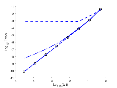
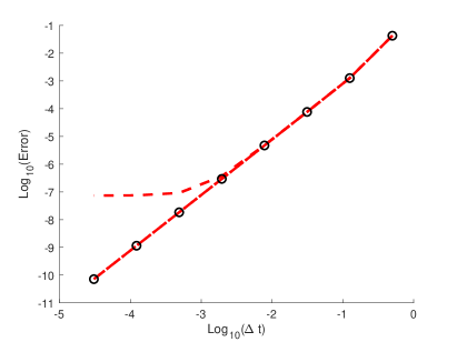
Figure 4: The Lobatto method with various implementations. The dashed line is a low-precision implementation, the dotted line is the naive mixed precision implementation (22), and the dash-dot line is the corrected mixed precision implementation (23). Left: half precision $\epsilon=O(10^{-4})$, Right: single precision $\epsilon=O(10^{-8})$.

In Figure 4 we show the half-precision (left) and single-precision (right) results of the various implementations of the Lobatto IIIC method. The errors from the low precision implementation are shown by a dashed line which starts off with slope $\sigma=2$ and very quickly becomes horizontal, as expected from the error analysis which predicts $Error_{LP}=O(\Delta t^{2})+O(\epsilon).$ The errors from the naive mixed-precision implementation (22) are shown by a dotted line which has slope $\sigma=2$ for $\epsilon=O(10^{-8})$, but has slope $\sigma=1$ for $\epsilon=O(10^{-4})$, which matches the predicted error $Error_{MP}=O(\Delta t^{2})+O(\epsilon\Delta t).$ What is happening here is that for the half precision implementation the term $O(\epsilon\Delta t)$ dominates early on, whereas for the single precision implementation we observe the $O(\Delta t^{2})$ convergence because $\Delta t$ is large compared to $\epsilon$. (For the single precision implementation the dotted line is hidden by the dash-dot line). Finally, the corrected mixed-precision method (23) has errors (shown in a dash-dot line) that are second order and that match the full-precision implementation (black circles).

4.2 Third order novel methods

The framework presented in Section 3 can not only be used to analyze naive mixed-precision implementations of existing methods and corrections to such methods, but to devise new methods. In this section we present examples of two methods that were developed to satisfy the order (10) and perturbation conditions (11) in Section 3.1 to high order. Both methods are four-stage third order methods. The first method, presented in Subsection 4.2.1, is not A-stable, and is third order with high order perturbation errors:

$$Error=O(\Delta t^{3})+O(\epsilon\Delta t^{3}).$$

The second method, presented in Subsection 4.2.2, is a perturbation of the four-stage third order L-stable method in [6], and so is A-stable. However, its perturbation errors are not as high order:

$$Error=O(\Delta t^{3})+O(\epsilon\Delta t^{2}).$$

The difference between these methods is evident in Figure 5. The errors for the mixed precision implementation of Method 4s3pA (Figure 5, left) are shown in dotted lines (blue for for half precision, and red for single precision). The mixed precision errors match the corresponding low-precision errors initially, but as $\Delta t$ gets smaller, the mixed precision errors match with the double-precision errors. For the A-stable Method 4s3pB (Figure 5, right) this is also true when considering the mixed precision method with $\epsilon=O(10^{-8})$. However, the mixed precision method with $\epsilon=O(10^{-4})$ does not match the double precision errors, even as $\Delta t$ gets small.

4.2.1 A four-stage third order mixed-precision method

This method, referred to as Method 4s3pA is given by the following coefficients:

The matrix $A$ is

$$a_{21}=0.211324865405187,\;\;a_{31}=0.709495523817170,\;\;a_{32}=-0.865314250619423,$$

$$a_{41}=0.705123240545107,\;\;a_{42}=0.943370088535775,\;\;a_{43}=-0.859818194486069,$$

$A^{\epsilon}$ has coefficients

$$a^{\epsilon}_{11}=0.788675134594813,\;\;a^{\epsilon}_{31}=0.051944240459852,\;\;a^{\epsilon}_{33}=0.788675134594813,$$

and the vectors are given by

$$b=(0,\frac{1}{2},0,\frac{1}{2}),\;\;\;\;b^{\epsilon}=(0,0,0,0).$$

4.2.2 A four-stage third order A-stable mixed-precision method

This A-stable method, referred to as Method 4s3pB is given by the following coefficients: For this A-stable method, $A$ is given by

$$a_{21}=2.543016042796356\;\;a_{31}=2.451484396921318,\;\;a_{32}=0.024108961241221,$$

$$a_{41}=2.073861819468268\;\;a_{42}=2.367724727682735\;\;a_{43}=1.711868223075524,$$

$A^{\epsilon}$ is

$$a^{\epsilon}_{11}=a^{\epsilon}_{22}=a^{\epsilon}_{33}=a^{\epsilon}_{44}=0.5,$$

$$a^{\epsilon}_{21}=-2.376349376129689,\;\;a^{\epsilon}_{31}=-2.951484396921318,\;\;a^{\epsilon}_{32}=0.475891038758779,$$

$$a^{\epsilon}_{41}=-0.573861819468268,\;\;a^{\epsilon}_{42}=-3.867724727682735,\;\;a^{\epsilon}_{43}=-1.211868223075524,$$

and

$$b=\left(\frac{3}{2},-\frac{3}{2},\frac{1}{2},\frac{1}{2}\right),\;\;\;\;b^{\epsilon}=\left(0,0,0,0\right).$$

This method is a perturbation the four-stage third order L-stable method in [6].

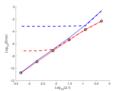
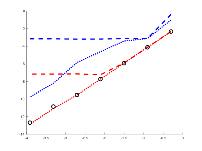
Figure 5: The four stage third order method given in Sections 4.2.1 (Method 4s3pA, left) and 4.2.2 (Method 4s3pB, right). The half-precision implementation ($\epsilon=O(10^{-4})$) is shown as a blue dashed line and the single-precision implementation $\epsilon=O(10^{-8})$ as a red dashed line. The mixed precision implementation with $\epsilon=O(10^{-4})$ is shown with a dotted blue line, and the mixed precision implementation with $\epsilon=O(10^{-8})$ is shown with a dotted red line. The double precision implementation is shown for reference with black dots.

4.3 A method that satisfies the simplified order conditions

In all of the above we considered methods that satisfied the perturbation conditions 11, that apply even when $\tau$ is not a well-behaved function. In this section, we devise a method that satisfies the less restrictive order conditions 12, that apply only when $\tau$ is well-behaved. This method, Method 4s3pC is given by the coefficients

$$a_{21}=-0.050470366527530,\;\;a_{31}=0.368613367355336,\;\;a_{32}=0.273504374252976,$$

$$a_{41}=1.803794668975043,\;\;a_{42}=0.097485042980759,\;\;a_{43}=-1.895660952342050.$$

$$a^{\epsilon}_{11}=0.511243008730995,\;\;a^{\epsilon}_{21}=-1.999347282862640,\;\;a^{\epsilon}_{22}=1.957161067302390,$$

$$a^{\epsilon}_{31}=0.443312893511937,\;\;a^{\epsilon}_{32}=-0.573131033672219,\;\;a^{\epsilon}_{33}=0.128283796414019,$$

$$a^{\epsilon}_{42}=-0.160330320741428,\;a^{\epsilon}_{43}=0.579597314161362,\;a^{\epsilon}_{44}=1.484688928981990,$$

$$a^{\epsilon}_{41}=-2,\;\;\;b^{\epsilon}=(0,0,0,0),$$

$$b=(0.002837446974069,\;\;0.336264433650450,\;\;0.806376720267787,\;\;-0.145478600892306).$$

When we have a well-behaved $\tau$, this method gives errors of the form

$$Error=O(\Delta t^{3})+O(\epsilon\Delta t^{3}).$$

However, $\tau$ is not well-behaved, this method gives error of the form

$$Error=O(\Delta t^{3})+O(\epsilon\Delta t^{2}).$$

Figure 6: Methods 4s3pC and 4s3pA for time evolution of the diffusion equation. The magenta dashed line is Method 4s3pC with $F$ resulting from a Fourier spectral method approximation to $u_{xx}$, and $F^{\epsilon}$ resulting from a second order centered difference approximation to $u_{xx}$. The dashed blue line is Method 4s3pC with $F$ resulting from a double precision implementation of a Fourier spectral method approximation to $u_{xx}$, and $F^{\epsilon}$ resulting from a half precision ”chopping” of the Fourier spectral method approximation. The dotted blue line is Method 4s3pA for this same scenario. The double precision implementation with a Fourier spectral method approximation is shown for reference with black circles.

We test this problem on the diffusion equation

$$u_{t}=u_{xx}$$

on $x\in(0,2\pi)$ with initial conditions $u(x,0)=sin(x)$ and periodic boundaries.

To discretize the spatial derivative we use a high resolution Fourier spectral method for $F$. For the $F^{\epsilon}$, we consider two different approaches. In the first approach, we use the low resolution centered difference scheme for $u_{xx}$ to evaluate $F^{\epsilon}$. This is a highly sensitive process, and a careful stability analysis must be carried out with the two different operators, so we do not recommend trying this approach in general without rigorous justification. We use it here only to illustrate the effect of using different resolution methods in our perturbed Runge–Kutta framework. We show in Figure 6, that using Method 4s3pC on the method where $F^{\epsilon}$ is given by a centered difference approximation (i.e. a well-behaved $\tau$) results, as expected, in an error of $Error=O(\Delta t^{3})+O(\epsilon\Delta t^{3})$ (magenta dashed line).

For comparison, we show a low precision (using the chop command) approximation of the Fourier spectral method for $F^{\epsilon}$. Recall that Method 4s3pC was designed to work with a well behaved $\tau$. In the case where we approximate $u_{xx}$ with the Fourier spectral method for $F$ and with the centered difference scheme for $F^{\epsilon}$, we can show that the difference between these is a well-behaved function. Using Method 4s3pC with the mixed precision approach with $\epsilon=10^{-4}$ (dashed blue line) results in an error that is initially third order and reduces to second order as $\Delta t$ gets smaller. This matches our expected error $Error=O(\Delta t^{3})+O(\epsilon\Delta t^{2})$ when $\tau$ is not well-behaved. Compare this with the performance of Method 4s3pA, which was designed to work with badly behaved $\tau$; we see that these errors start at higher than third order, and settle down to third order behavior. The convergence of this mixed precision method is of the same order as the low/high resolution method, and of the high resolution method, but it has a larger error constant.

5 Conclusions

In this work we presented a framework for the error analysis of perturbations of Runge–Kutta methods. In particular, we investigate the case where perturbations arise from a mixed precision implementation of Runge–Kutta methods. This is particularly useful for implicit methods, where is implicit evaluation is computationally costly. Using this framework, we investigate mixed precision implementations of existing methods and a correction approach that improves the errors, and devised new methods that have favorable scheme error and perturbation error properties. Numerical demonstrations illustrate the performance of these methods as described by the theory. Although this mixed precision approach was designed for implicit Runge–Kutta schemes, it can also be applied when repeated explicit function evaluation is expensive, and storage of the computed values is not possible due to the size of the problem.

In the case where we use a chopping routine to emulate a low precision operator, we developed more stringent conditions on the method to handle the unbounded behavior of the truncation operator. The framework developed holds for more general perturbations than mixed precision calculations: we also presented simplified order conditions that are applicable when the perturbation function $\tau$ is well-behaved. These methods can thus be extended to many types of perturbations. While in this work we treat epsilon as a single constant upper bound, in future work we will generalize this approach to design methods with varying orders of epsilon.

References

• [1] A. Abdelfattah, H. Anzt, E.G. Boman, E. Carson, T. Cojean, J. Dongarra, M. Gates, T. Grutzmacher, N.J. Higham, S. Li, N. Lindquist, Y. Liu, J. Loe, P. Luszczek, P. Nayak, S. Pranesh, S. Rajamanickam, T. Ribizel, B. Smith, K. Swirydowicz, S. Thomas, S. Tomov, Y.M. Tsai, I. Yamazaki, U.M. Yang, “A Survey of Numerical Methods Utilizing Mixed Precision Arithmetic,” arXiv:2007.06674,2020.
• [2] R. Alexander, Diagonally implicit Runge-Kutta methods for stiff O.D.E.s, SIAM Journal on Numerical Analysis (1977) 14(6) pp. 1006-1021.
• [3] U. Ascher, S. Ruuth, and B. Wetton, Implicit-explicit methods for time-dependent partial differential equations, SIAM Journal on Numerical Analysis (1995) 32, p. 797–823.
• [4] C. A. Kennedy and M. H. Carpenter, Additive Runge–Kutta schemes for convection–diffusion–reaction equations, Applied Numerical Mathematics (2003) 44:1-2, pp. 139-181.
• [5] S. E. Field, S. Gottlieb, Z. J. Grant, L. F. Isherwood, G. Khanna, A GPU-accelerated mixed-precision WENO method for extremal black hole and gravitational wave physics computations, https://arxiv.org/abs/2010.04760.
• [6] E. Hairer and G. Wanner, Solving Ordinary Differential Equations II, Stiff and Differential-Algebraic Problems. Springer, 1991.
• [7] N. J. Higham and S. Pranesh, Simulating low precision floating-point arithmetic, SIAM Journal on Scientific Computing (2019), 41:5, pp. C585-C602.
• [8] I. Higueras, D.I. Ketcheson, and T.A. Kocsis, Optimal Monotonicity-Preserving Perturbations of a Given Runge–Kutta Method, Journal of Scientific Computing (2018) 76, 1337–1369 .
• [9] D. I. Ketcheson, M. Parsani , Z. J. Grant , A. J. Ahmadia, and H. Ranocha RK-Opt: A package for the design of numerical ODE solvers, Journal of Open Source Software (2020), 5(54), 2514, https://doi.org/10.21105/joss.02514
• [10] T. Kouya, Practical Implementation of High-Order Multiple Precision Fully Implicit Runge-Kutta Methods with Step Size Control Using Embedded Formula, https://arxiv.org/abs/1306.2392
• [11] S. P. Norsett, G. Wanner (1981) Perturbed collocation and Runge-Kutta methods, Numerische Mathematik (1981) 38:193-208.
• [12] A. Sandu and M. Gunther, A Generalized-Structure Approach to Additive Runge–Kutta Methods, SIAM Journal on Numerical Analysis (2015) 53(1), pp. 17–42.