Minimal controllability time for systems with nonlinear drift under a compact convex state constraint

Abstract

In this paper we estimate the minimal controllability time for a class of non-linear control systems with a bounded convex state constraint. An explicit expression is given for the controllability time if the image of the control matrix is of co-dimension one. A lower bound for the controllability time is given in the general case. The technique is based on finding a lower dimension system with the similar controllability properties as the original system. The controls corresponding to the minimal time, or time close to the minimal one, are discussed and computed analytically. The effectiveness of the proposed approach is illustrated by a few examples.

1 Introduction

In this paper we consider the question of controllability for systems with non-linear drift, linear control, and state constraint. The state of the system is required to stay within certain bounded convex set.

The proposed technique consists in considering an auxiliary system of lower dimension which has similar controllability properties. This allows to derive lower bounds on the controllability time. For the case when the range of the control matrix has co-dimension one (that is, the image of the control matrix is a linear space of dimension one less than the entire state space), an explicit expression for the controllability time is given. Using similar technique, in the complementary case we give a lower bound on the controllability time. The main idea behind our analysis is that the controllability time for the original system can be expressed in terms of the controllability time for a lower dimension system. The present work is inspired and partially motivated by [6].

As in [6] we focus on controllability with a state constraint, but without control constraints, that is, every $L^{\infty}$ control is allowed. Some of the main techniques in [6] are Brunkovsky normal form for a linear equation, and Goh transformation. In the present paper we too use equivalent systems to derive properties of the minimal controllability time, although our approach differs as the alternative system we arrive to is obtained via orthogonal projection rather than transforming the system into a normal form.

Control systems with state constraints is a challenging topic for mathematical analysis that has seen a gradual rise in interest over the recent years. Quoting from [6], “Controllability under state constraints has not been much investigated in the literature, certainly due to the difficulty of the question, even for linear control systems.” The main object of [12] is to give conditions on a closed set $S$ so that every point sufficiently close to $S$ can be steered into $S$ within a small time by an admissible control. The authors call this property small-time local attainability. The control system in [12] is non-linear. A similar problem in stochastic settings was studied in [1]. The estimators for systems with linear and non-linear state constraints are surveyed in [9], see also [4]. In [5], systems with linear state constraint and with convex cone signal constraint are considered. A geometric necessary and sufficient small time controllability condition is formulated in terms of involved constraining sets. Controllability of the fractional systems with constrained delayed controls is treated in [11, 10].

We work in a framework similar to [6]. The main differences in the models between [6] and the present paper are that our system is non-linear, and that we work only with bounded convex constraint sets. In [6] the focus is on whether the system is controllable under the state constraint, and whether the controllability time is positive. Meanwhile in the present work we mostly address the questions of estimating and explicitely computing the controllability time for non-linear systems in arbitrary dimension. It was noted in [6] that obtaining an explicit expression or even an estimate for the controllability time remained an open problem for linear system in dimensions higher than two. Here we provide such expressions and estimates in a wide range of cases encompassing bounded convex state constraints for more general non-linear systems. The main idea behind our analysis is to show a certain equivalence between the original system and a non-linear one with a lower dimension. This is achieved by decomposing $\mathbb{R}^{n}$ into an orthogonal sum of ‘fast’ directions (those in the range of the control matrix) and ‘slow’ directions (the orthogonal complement). Under the assumption of convexity the ‘fast’ directions are usually straightforward to handle, and the focus of our analysis is on the ‘slow’ ones.

The paper is organized as follows. In Section 2 we describe the non-linear control system analyzed in this paper. In Section 3 we show that the controllability time of the original system is related to the controllability time of a lower dimension system. The estimates on the controllability time and an exact expression are also derived in Section 3. In Section 4 we discuss some numerical examples. The concluding remarks are collected in Section 5.

2 Problem formulation

We consider the system governed by the equation

$$\dot{y}(t) =F(y(t))+Bu(t),$$ (1)

where $y\in\mathbb{R}^{n}$ is the state vector, $F:\mathbb{R}^{n}\to\mathbb{R}^{n}$ is a continuous vector field, $B$ is $n\times m$ matrix of rank $m$ with $m<n$. Henceforth we identify a matrix with the linear operator it induces. System (1) is endowed with the additional constraint

$$y(t)\in\mathcal{C},$$

where $\mathcal{C}\subset\mathbb{R}^{n}$ is a bounded convex set. We always assume the interior $\mathcal{C}^{\mathrm{o}}$ of $\mathcal{C}$ to be not empty.

Let $y^{0},y^{1}\in\mathcal{C}^{\mathrm{o}}$. We define the smallest time to reach one point from another as

$$\begin{split}T_{\mathcal{C}}(y^{0},y^{1})=\inf\{T>0:\text{there exists }u\in L^{\infty}([0,T],\mathbb{R}^{m})\text{ s.t. }y(t)\in\mathcal{C}\text{ for }t\in[0,T],\text{ and }\\ \eqref{the model}\text{ holds with }y(0)=y^{0},y(T)=y^{1}\}.\end{split}$$ (2)

Here and throughout, we assume that $y^{0},y^{1}\in\mathcal{C}^{\mathrm{o}}$ and adopt the convention $\inf\varnothing=+\infty$. If $T_{\mathcal{C}}(y^{0},y^{1})<\infty$, we say that $y^{1}$ is reachable from $y^{0}$ with the state constraint $\mathcal{C}$. We avoid the initial and final points being on the boundary ($y^{0}\in\partial\mathcal{C}$ or $y^{1}\in\partial\mathcal{C}$), because this case would require additional technical assumptions. Indeed, for some systems any solution to (1) started from some $y^{0}\in\partial\mathcal{C}$ leaves $\mathcal{C}$ immediately. Similarly, for some $y^{1}\in\partial\mathcal{C}$ any solution reaching $y^{1}$ may have to come from the complement of $\mathcal{C}$. On the other hand, if for $y^{0}\in\partial\mathcal{C}$ there exists a signal $u$ such that the solution to (1) belongs to $\mathcal{C}^{\mathrm{o}}$ for small $t>0$, then our results are applicable because we can take a new starting point in the interior of $\mathcal{C}$ after an arbitrary small delay.

Let us see in a simple case a state constraint affects the controllability time. Let $n=2$, $m=1$, $A=\begin{pmatrix}0&-1\\ 1&0\end{pmatrix}$, $B=\begin{pmatrix}1\\ 0\end{pmatrix}$, $F(y)=Ay$, so that the system is

$$\begin{cases}\begin{aligned} \dot{y_{1}}(t)&=-y_{2}(t)+u(t),\\ \dot{y_{2}}(t)&=y_{1}(t).\end{aligned}\end{cases}$$ (3)

The Kalman condition is satisfied here, so the state $(0,1)^{\top}$ (here and elsewhere, $\top$ indicates transposition) can be reached from $(0,0)^{\top}$ in an arbitrary time if there is no constraint. Assume we also require that for a constant $C>0$,

$$|y_{1}(t)|<C.$$

Then if system (3) reaches $(0,1)^{\top}$ from $(0,0)^{\top}$ at time $T>0$, we have

$$1=y_{2}(T)-y_{2}(0)=\int\limits_{0}^{T}y_{1}(t)dt\leq CT,$$

and hence $T\geq\frac{1}{C}$. This means that the controllability time cannot be made arbitrary small under the state constraint, even though every state within the constraint set is reachable from any other. More examples can be found in [6].

Let $H=(\text{ran}(B))^{\perp}$ be the orthogonal complement to the range of $B$ in $\mathbb{R}^{n}$. The space $H$ represents the ‘slow’ directions mentioned in the introduction. Note that $\dim H=n-m$. For a subspace $G$, let $P_{G}y$ be the orthogonal projection of $y$ on $G$ and for a map $M:\mathbb{R}^{n}\to\mathbb{R}^{n}$, $M_{G}(y):=P_{G}M(y)$. Denote also by $\mathcal{C}_{H}$ the orthogonal projection of $\mathcal{C}$ on $H$. For a map $M:X\to Y$ and a set $\mathcal{Q}\subset X$, the image of $\mathcal{Q}$ under $M$ is defined as $M\mathcal{Q}=\{Mx:x\in\mathcal{Q}\}\subset Y.$

We make the following assumptions on $F$ and $\mathcal{C}$.

Condition 2.1.

The set $\mathcal{C}$ is a bounded convex subset of $\mathbb{R}^{n}$ with a smooth $C^{1}$ boundary.

Condition 2.2.

The function $F$ is continuous and Lipschitz with the Lipschitz constant $L_{{F}}>0$, that is, ${|F(x)-F(y)|\leq L_{F}|x-y|}$ for all $x,y\in\mathbb{R}^{n}$.

We also make the following technical assumptions.

Condition 2.3 (measurable selection).

There exists a Borel measurable map $f$ defined on

$$\mathcal{D}_{f}:=\{(h_{1},h_{2})\in H\times H:\text{ for some }h^{\perp}\in H^{\perp},h_{1}=F_{H}(h_{2}+h^{\perp})\text{ and }h_{2}+h^{\perp}\in\mathcal{C}\}$$

such that for every $(h_{1},h_{2})\in\mathcal{D}_{f}$,

$$h_{1}=F_{H}(h_{2}+f(h_{1},h_{2})).$$

Condition 2.3 is a technical assumption which we expect to hold in all reasonable cases. The measurable selection property is closely related to the uniformization problem in descriptive set theory [8]. In particular, if for each $(h_{1},h_{2})\in\mathcal{D}_{f}$ the set

$$S_{(h_{1},h_{2})}=\{h^{\perp}\mid h_{1}=F_{H}(h_{2}+h^{\perp})\text{ and }h_{2}+h^{\perp}\in\mathcal{C}\}$$

is at most countable or is of positive Lebesgue measure, Condition 2.3 is satisfied [13, 3].

For vectors $v_{1},v_{2}$ of equal dimension denote by $[v_{1},v_{2}]$ their closed convex hull. For $x\in\mathbb{R}^{\mathrm{d}}$, $\mathrm{d}\in\mathbb{N}$, and $r>0$, let $\mathcal{B}(x,r)$ be the closed ball $\{y\in\mathbb{R}^{\mathrm{d}}\mid|y-x|\leq r\}$. In particular, $\mathcal{B}(x,0)=\{x\}$.

3 Reduction to a lower dimension problem

One of the aims of the present work is to find another representation of $T_{\mathcal{C}}(y^{0},y^{1})$ as a certain time related to a problem in lower dimension. To this end we introduce auxiliary dynamics defined by the inclusion

$$\dot{z}(t)\in F_{H}\left((z(t)+H^{\perp})\cap\mathcal{C}\right),$$ (4)

where the state $z$ takes values in $\mathbb{R}^{\dim(H)}$. We now define the controllability time for (4) by

$$\begin{split}\overline{T}_{\mathcal{C}}(y^{0},y^{1})=\inf\big{\{}T:\text{there exists }z(t)\in C([0,T],H)\text{ s.t. }\eqref{charade}\text{ holds with }\\ z(0)=P_{H}y^{0},z(T)=P_{H}y^{1}\big{\}}.\end{split}$$ (5)

Denote by $L^{0}(X,Y)$ the set of all measurable maps from $X$ to $Y$. We also define another auxiliary equation with constraints

$$\begin{gathered}\dot{z}(t)=F_{H}(z(t)+h^{\perp}(t))\\ z(t)+h^{\perp}(t)\in\mathcal{C},\ \ \ h^{\perp}(t)\in H^{\perp},\end{gathered}$$ (6)

and the respective controllability time

$$\begin{split}\widehat{T}_{\mathcal{C}}(y^{0},y^{1})=\inf\big{\{}T:\text{there exists }z(t)\in C([0,T],H),h^{\perp}(t)\in L^{0}([0,T],H^{\perp})\text{ s.t. }z(0)=P_{H}y^{0},\\ z(T)=P_{H}y^{1},\text{ and \eqref{system hat} holds}\big{\}}.\end{split}$$

The relation between $T_{\mathcal{C}}(y^{0},y^{1})$, $\overline{T}_{\mathcal{C}}(y^{0},y^{1})$, and $\widehat{T}_{\mathcal{C}}(y^{0},y^{1})$ is clarified in this section. It is worth noting that we are mostly interested in $T_{\mathcal{C}}(y^{0},y^{1})$, whereas $\overline{T}_{\mathcal{C}}(y^{0},y^{1})$ and $\widehat{T}_{\mathcal{C}}(y^{0},y^{1})$ play an auxiliary role (although they might be of interest in their own right).

Lemma 3.4.

Let $y^{0},y^{1}\in C^{\mathrm{o}}$. It holds that

$$\begin{split}\widehat{T}_{\mathcal{C}}(y^{0},y^{1})=\overline{T}_{\mathcal{C}}(y^{0},y^{1}).\end{split}$$ (7)

Proof. Since the infimum taken over a smaller set is larger, $\widehat{T}_{\mathcal{C}}(y^{0},y^{1})\geq\overline{T}_{\mathcal{C}}(y^{0},y^{1})$. Let $\varepsilon>0$ be a small number. There exists $T\leq\overline{T}_{\mathcal{C}}(y^{0},y^{1})+\varepsilon$ and $z(t)\in C([0,T],H)$ such that

$$z(0)=P_{H}y^{0},\ \ z(T)=P_{H}y^{1},$$

and (4) holds. Set

$$g^{\perp}(t):=f(\dot{z}(t),z(t)),$$ (8)

where $f$ is the map from Condition 2.3. Note that $\dot{z}(t):[0,T]\to H$ is Lebesgue measurable, and hence $g:[0,T]\to H^{\perp}$ is Lebesgue measurable as well. Also,

$$\dot{z}(t)=F_{H}(z(t)+f(\dot{z}(t),z(t)))=F_{H}(z(t)+g^{\perp}(t)),$$

and hence $\widehat{T}_{\mathcal{C}}(y^{0},y^{1})\leq T\leq\overline{T}_{\mathcal{C}}(y^{0},y^{1})+\varepsilon$. Since $\varepsilon>0$ is arbitrary, the proof is complete. ∎

Lemma 3.5.

Let $y^{0},y^{1}\in C^{\mathrm{o}}$. It holds that

$$\begin{split}\overline{T}_{\mathcal{C}}(y^{0},y^{1})\leq T_{\mathcal{C}}(y^{0},y^{1}).\end{split}$$ (9)

Proof. The statement is a consequence of the fact that the infimum taken over a larger set is smaller. ∎

Remark 3.6.

Lemma 3.4 and Lemma 3.5 do not require Condition 2.1: their conclusions hold for arbitrary measurable $\mathcal{C}$.

For $h,h_{0},h_{1}\in H$, $h_{0}\neq h_{1}$, we define

$$s(h,h_{0},h_{1})=\frac{\sup\langle F_{H}((h+H^{\perp})\cap\mathcal{C}),h_{1}-h_{0}\rangle}{|h_{1}-h_{0}|},$$

where

$$\langle F_{H}((h+H^{\perp})\cap\mathcal{C}),h_{1}-h_{0}\rangle=\{\langle x,h_{1}-h_{0}\rangle\mid x\in F_{H}((h+H^{\perp})\cap\mathcal{C})\}.$$ (10)

The next theorem gives a way to compute $T_{\mathcal{C}}(y^{0},y^{1})$ in the case $m=n-1$, i.e. when the range of $B$ has co-dimension one.

Theorem 3.7.

Let $\dim H=1$ and $h_{0}\neq h_{1}$, where $h_{i}=P_{H}y^{i}$, $i=1,2$.

• $(i)$ if $s(h,h_{0},h_{1})>0$ for all $h\in[h_{0},h_{1}]$, then $T_{\mathcal{C}}(y^{0},y^{1})=\overline{T}_{\mathcal{C}}(y^{0},y^{1})<\infty$, and

  $$T_{\mathcal{C}}(y^{0},y^{1})=\int\limits_{h\in[h_{0},h_{1}]}\frac{dh}{s(h,h_{0},h_{1})}.$$ (11)

  In particular, the integral in (11) is finite.

• $(ii)$ if $s(h_{2},h_{0},h_{1})\leq 0$ for some $h_{2}\in[h_{0},h_{1}]$, then $T_{\mathcal{C}}(y^{0},y^{1})=\overline{T}_{\mathcal{C}}(y^{0},y^{1})=\infty$.

Proof. We start with $(i)$. We begin with the auxiliary claim

$$\overline{T}_{\mathcal{C}}(y^{0},y^{1})=\int\limits_{h\in[h_{0},h_{1}]}\frac{dh}{s(h,h_{0},h_{1})}.$$ (12)

Let $s(h,h_{0},h_{1})>0$ for all $h\in[h_{0},h_{1}]$. By definition of $s(h,h_{0},h_{1})$ and since $F$ is continuous, we have in fact $\inf\limits_{h\in[h_{0},h_{1}]}s(h,h_{0},h_{1})>0$. Hence the integral in (11) is well defined and finite. For a small positive $\delta<\frac{1}{2}\inf\limits_{h\in[h_{0},h_{1}]}s(h,h_{0},h_{1})$, the system

$$\begin{cases}z(0)=P_{H}y^{0},\\ z(T)=P_{H}y^{1},\\ \dot{z}(t)\in F_{H}\left((z(t)+H^{\perp})\cap\mathcal{C}\right),\\ T>0\end{cases}$$ (13)

has a solution satisfying $\frac{\langle\dot{z}(t),h_{1}-h_{0}\rangle}{|h_{1}-h_{0}|}>s(z(t),h_{0},h_{1})-\delta$ with

$$T^{(\delta)}=\int\limits_{h\in[h_{0},h_{1}]}\frac{dh}{s(h,h_{0},h_{1})-\delta}.$$ (14)

Taking the limit $\delta\downarrow 0$, we get by the dominated convergence theorem

$$\overline{T}_{\mathcal{C}}(y^{0},y^{1})\leq\liminf\limits_{\delta\downarrow 0}T^{(\delta)}=\int\limits_{h\in[h_{0},h_{1}]}\frac{dh}{s(h,h_{0},h_{1})}.$$ (15)

Using Lemma A1 in the Appendix, we now prove the reverse inequality $\overline{T}_{\mathcal{C}}(y^{0},y^{1})\geq\int\limits_{h\in[h_{0},h_{1}]}\frac{dh}{s(h,h_{0},h_{1})}$. Note that

$$\begin{gathered}\frac{\langle\dot{z}(t),h_{1}-h_{0}\rangle}{|h_{1}-h_{0}|}\leq\sup\left\langle F_{H}\left((z(t)+H^{\perp})\right),h_{1}-h_{0}\right\rangle\leq{s}(z(t),h_{0},h_{1})\end{gathered}$$

and $\frac{\langle\dot{z}(T)-h_{0},h_{1}-h_{0}\rangle}{|h_{1}-h_{0}|}=|h_{1}-h_{0}|$. Applying Lemma A1 with $M=|h_{1}-h_{0}|$, $f(t)=\frac{\langle z(t)-h_{0},h_{1}-h_{0}\rangle}{|h_{1}-h_{0}|}$, and

$$g(v)=s\left(h_{0}+\frac{v}{|h_{1}-h_{0}|}(h_{1}-h_{0}),h_{0},h_{1}\right),\ \ \ v\in[0,|h_{1}-h_{0}|],$$

we get

$$\overline{T}_{\mathcal{C}}(y^{0},y^{1})\geq\int\limits_{0}^{|h_{1}-h_{0}|}\frac{dv}{s(h_{0}+\frac{v}{|h_{1}-h_{0}|}(h_{1}-h_{0}),h_{0},h_{1})}=\int\limits_{h\in[h_{0},h_{1}]}\frac{dh}{s(h,h_{0},h_{1})}.$$ (16)

Thus, (12) is proved. Next we proceed with the proof of $T_{\mathcal{C}}(y^{0},y^{1})=\overline{T}_{\mathcal{C}}(y^{0},y^{1})$. Recall that by Lemma 3.4, $\widehat{T}(y^{0},y^{1})=\overline{T}(y^{0},y^{1})$. Take $\varepsilon>0$. There exist $T<\widehat{T}(y^{0},y^{1})+\varepsilon$, $z\in C([0,T],H)$, and $h^{\perp}\in L^{0}([0,T],H^{\perp})$ such that (6) holds, $P_{H}y^{0}=z(0)$, and $P_{H}y^{1}=z(T)$. Take now a small $\delta>0$. Since $\mathcal{C}$ is bounded and convex, it is possible to choose $h^{c}\in C^{1}([0,T],H^{\perp})$ (the space of continuously differentiable functions) in such a way that $|h^{\perp}-h^{c}|_{L^{1}([0,T],H^{\perp})}<\delta$ and for $t\geq 0$, $z^{c}(t)+h^{c}(t)\in\mathcal{C}$, where $z^{c}(t)$ is the the solution to

$$\dot{z}^{c}(t)=F_{H}(z^{c}(t)+h^{c}(t)),\ \ \ z^{c}(0)=P_{H}y^{0}.$$ (17)

Let $y^{c}(t)=z^{c}(t)+h^{c}(t)$. Note that $y^{c}$ is a solution to (1). Subtracting (17) from (6) we get in the integral form

$$z(t)-z^{c}(t)=\int\limits_{0}^{{t}}F_{H}(z(t)-z^{c}(t))dt+\int\limits_{0}^{{t}}F_{H}(h^{\perp}(t)-h^{c}(t))dt,$$

hence

$$|z(t)-z^{c}(t)|\leq L_{F}\int\limits_{0}^{t}|z(t)-z^{c}(t)|dt+{L_{F}}T\delta,$$ (18)

where $L_{F}$ is the Lipschitz constant for $F$. By Grönwall’s inequality from (18) we obtain

$$|z(t)-z^{c}(t)|\leq L_{F}Te^{L_{F}T}\delta,\ \ \ t\in[0,T].$$ (19)

In particular,

$${|h_{1}-z^{c}(T)|}=|z(T)-z^{c}(T)|\leq L_{F}Te^{L_{F}T}\delta$$ (20)

Recall that we took $T<\widehat{T}(y^{0},y^{1})+\varepsilon$. Since $\mathcal{C}$ is compact and convex, $\inf\limits_{h\in[h_{0},h_{1}]}{s(h,h_{0},h_{1})}>0$. Let $s_{m}>0$ be such that

$$s(h,h_{0},h_{1})>s_{m},\ \ \ h\in[h_{0},h_{1}].$$ (21)

Without loss of generality we can assume that

$$\langle z^{c}(T)-h_{0},h_{1}-h_{0}\rangle <\langle h_{1}-h_{0},h_{1}-h_{0}\rangle,$$ (22)

$$\ \ \ \langle F(z^{c}(T)+h^{c}(T)),h_{1}-h_{0}\rangle =s_{m}>0$$ (23)

and that $\delta>0$ is so small that there exists $r>|h_{1}-z^{c}(T)|$ such that for all $y$ with $|y-z^{c}(T)-h^{c}(T)|<r$,

$$\langle F(y),h_{1}-h_{0}\rangle>\frac{1}{2}s_{m}$$ (24)

and the ball

$$\{y\in\mathbb{R}^{n}\mid|y-z^{c}(T)-h^{c}(T)|\leq r\}\subset\mathcal{C}^{\mathrm{o}}.$$ (25)

Indeed, if the first inequality in (22) does not hold, then we can go back in time. More precisely, we can replace $z^{c}(T)$ with $z^{c}(T-\Delta)$ for a small $\Delta>0$ so that both (20) and (22) hold; then, since $s(h,h_{0},h_{1})>0$ for $h\in[h_{0},h_{1}]$, for some $h^{\perp,2}$ with $z^{c}(T)+h^{\perp,2}\in\mathcal{C}$ we have $\langle F(z^{c}(T)+h^{\perp,2}),h_{1}-h_{0}\rangle{>0}$, and therefore we can make the inequality in (23) hold true as well by modifying if necessary $h^{c}$ near $T-\Delta$ to ensure $h^{c}(T-\Delta)=h^{\perp,2}$. Finally, (24) and (25) are possible because $\mathcal{C}$ is compact and convex and $F$ is uniformly continuous on $\mathcal{C}$.

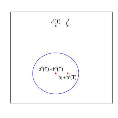
Figure 1: The plane $\mathcal{L}$. The radius of the blue circle is $r$.

It is possible to reach $y^{1}$ starting from $z^{c}(T)+h^{c}(T)$ in a short time interval $[T,T_{1}]$. Indeed, denote by $\mathcal{L}$ the two-dimensional plane spanning points $z^{c}(T)+h^{c}(T)$, $h_{1}+h^{c}(T)$, and $y^{1}$ (the case $h_{1}+h^{c}(T)=y^{1}$ is simpler and discussed below). The plane $\mathcal{L}$ is depicted on Figure 1. Note that $z^{c}(T)\in\mathcal{L}$ since $z^{c}(T)=(z^{c}(T)+h^{c}(T))+y^{1}-(h_{1}+h^{c}(T))$, and hence also $H\subset\mathcal{L}$. Let us only consider controls $u$ ensuring that $y(t)$ stays in $\mathcal{L}$, that is, $P_{\mathcal{L}^{\perp}}Bu(t)=-P_{\mathcal{L}^{\perp}}F(y(t))$, $t\geq T$. Denote by $\mathcal{K}$ a one-dimensional subspace of $\mathcal{L}$ orthogonal to $H$. Starting from $t=T$, we take $P_{\mathcal{K}}Bu(t)=-P_{\mathcal{K}}F(y(t))$ at the beginning, ensuring that $y(t)$ is moving on the interval $[z^{c}(T)+h^{c}(T),h_{1}+h^{c}(T)]$ toward $h_{1}+h^{c}(T)$ at a speed at least $s_{m}/2$.

At a time $\tau$ when $y(t)$ is near $h_{1}+h^{c}(T)$, we stop requiring $P_{\mathcal{K}}Bu(t)=-P_{\mathcal{K}}F(y(t))$ and instead take $P_{\mathcal{K}}Bu(t)=M(y^{1}-h_{1}-h^{c}(T))$ for a large number $M$. By an intermediate value theorem, for some $\tau>T$, $y(t)$ is going to pass through $y^{1}$ at a certain time $T_{1}$. By taking $\delta$ small and $M$ large, we can ensure that $T_{1}-T$ is small. Note that here it is important that $y^{1}$ is in the interior $\mathcal{C}^{\mathrm{o}}$, because otherwise even for large $M>0$, a trajectory of $y(t)$ hitting $y^{1}$ may cross the boundary of $\mathcal{C}$, violating the constraint condition.

In the case $h_{1}+h^{c}(T)=y^{1}$ we just require $P_{H^{\perp}}Bu(t)=-P_{H^{\perp}}F(y(t))$ for $t\geq T$, ensuring that $y(t)$ stays on the interval $[z^{c}(T)+h^{c}(T),h_{1}+h^{c}(T)]=[z^{c}(T)+h^{c}(T),y^{1}]$ and hits $y^{1}$.

We note here that in particular if $\langle P_{H}F(y^{1}),h_{1}-h_{0}\rangle<0$, it is important that $y^{1}\in\mathcal{C}^{\mathrm{o}}$, because the trajectory of $y(t)$ has to reach $y^{1}$ from ‘behind’, that is, from within the half-space $\left\{u\in\mathbb{R}^{n}:\langle u-h_{1},h_{1}-h_{0}\rangle>0\right\}$.

Therefore, $T_{\mathcal{C}}(y^{0},y^{1})=\widehat{T}_{\mathcal{C}}(y^{0},y^{1})=\overline{T}_{\mathcal{C}}(y^{0},y^{1})$, and $(i)$ follows from (12).

Having proved $(i)$, we now turn to $(ii)$. Let $h_{2}\in[h_{0},h_{1}]$ be such that $s(h_{2},h_{0},h_{1})\leq 0$. Since the boundary $\partial\mathcal{C}$ is assumed to be differentiable and $\mathcal{C}$ is convex, the Borel set valued map

$$[h_{0},h_{1}]\ni h\mapsto\mathcal{C}_{h}\in\mathscr{B}(H^{\perp})$$ (26)

defined by $\mathcal{C}_{h}=\{y\in\mathcal{C}\mid P_{H}y=h\}$ is Lipschitz continuous in Hausdorff distance (or Hausdorff metric, see e.g. [2]) with some constant $L_{1}$. Since $F$ is also Lipschitz continuous, it holds that

$$s(h,h_{0},h_{1})\leq(L_{F}+L_{1})|h-h_{2}|,\ \ \ h\in[h_{0},h_{2}].$$ (27)

It follows from (27) that any solution to (4) starting from $P_{H}y^{0}$ never reaches the location $h_{2}$: that is, for all $t\geq 0$,

$$\langle z(t)-h_{0},h_{1}-h_{0}\rangle<\langle h_{2}-h_{0},h_{1}-h_{0}\rangle.$$

Consequently, (13) has no solutions. Hence $\overline{T}_{\mathcal{C}}(y^{0},y^{1})=\infty$, and by Lemma 3.5, $T_{\mathcal{C}}(y^{0},y^{1})=\infty$. ∎

The purpose of following example is to demonstrate that the assumption $\dim H=1$ in Theorem 3.7 is necessary: without it the conclusion of the theorem need not be true.

Example 3.8.

Here we provide an example where all conditions of Theorem 3.7, $(i)$ are satisfied except $\dim H=1$, but the conclusions of $(i)$ are false, in particular,

$$\overline{T}_{\mathcal{C}}(y^{0},y^{1})=\widehat{T}_{\mathcal{C}}(y^{0},y^{1})\neq T_{\mathcal{C}}(y^{0},y^{1}).$$

Let $n=3$, $m=1$, $\mathcal{C}=[-2,2]^{3}$, $B:\mathbb{R}\to\mathbb{R}^{3}$, $Bu=(0,0,u)^{\top}$. Thus, $H=\{(\alpha,\beta,0)^{\top}\mid\alpha,\beta\in\mathbb{R}\}$, and $H^{\perp}=\{(0,0,\gamma)^{\top}\mid\gamma\in\mathbb{R}\}$. Note that $\dim H=2$. We impose the following conditions on $F$.

1. For $x\in\mathcal{C}$, $x\notin\Big{\{}(\alpha,0,1)\mid\alpha\in[-1,1]\Big{\}}\cup\Big{\{}(\alpha,0,0)\mid\alpha\in[-1,1]\Big{\}}$, we have $\langle F(x),(0,1,0)^{\top}\rangle>0$. Here and elsewhere, $\langle\cdot,\cdot\rangle$ is the scalar product in $\mathbb{R}^{n}$.

2. $F(\alpha,0,1)^{\top}=F(\beta,0,0)^{\top}=(1,0,0)^{\top}$ for $\alpha\in[-1,0]$, $\beta\in[0,1]$.

3. $F(\alpha,0,1)^{\top}=F(\beta,0,0)^{\top}=(-1,0,0)^{\top}$ for $\alpha\in[\frac{1}{2},1]$, $\beta\in[-1,-\frac{1}{2}]$.

Of course, many vector fields exist satisfying those conditions. Take now $y^{0}=(-1,0,1)^{\top}$ and $y^{1}=(1,0,0)^{\top}$. It is not difficult to see that $T_{\mathcal{C}}(y^{0},y^{1})=\infty$, since once the trajectory $y(t)$ of the solution to (1) leaves the segment $\{(\alpha,0,1)\mid\alpha\in[-1,1]\}$, the second coordinate of $y(t)$ becomes positive and stays positive forever: $\langle y(t),(0,1,0)^{\top}\rangle>0$. On the other hand, $\widehat{T}_{\mathcal{C}}(y^{0},y^{1})\leq 2$. Indeed, $z(t)=(-1+t,0,0)^{\top}\in H$ and

$$h^{\perp}(t)=\begin{cases}(0,0,1)^{\top},\ \ t<1,\\ (0,0,0)^{\top},\ \ t\geq 1,\end{cases}$$

give a solution to (6) with $z(0)=P_{H}y^{0}$ and $z(2)=P_{H}y^{1}$. Thus, $\widehat{T}_{\mathcal{C}}(y^{0},y^{1})\leq 2<\infty=T_{\mathcal{C}}(y^{0},y^{1})$. The equality $\widehat{T}_{\mathcal{C}}(y^{0},y^{1})=\overline{T}_{\mathcal{C}}(y^{0},y^{1})$ follows from Lemma 3.4. The example can of course be modified so that $T_{\mathcal{C}}(y^{0},y^{1})<\infty$ but still $T_{\mathcal{C}}(y^{0},y^{1})>2\geq\widehat{T}_{\mathcal{C}}(y^{0},y^{1})$. $\Diamond$

Example 3.9.

Let us also mention an annulus as an example where all conditions of Theorem 3.7 are satisfied except the convexity of $\mathcal{C}$, while the conclusions of Theorem 3.7 fail. Take $n=2$, $F((x_{1},x_{2})^{\top})\equiv(1,0)^{\top}$, $B=(0,1)^{\top}$,

$$\mathcal{C}=\left\{(x_{1},x_{2})^{\top}\middle|4\leq x_{1}^{2}+x_{2}^{2}\leq 16\right\},$$

$y^{0}=(-1,3)^{\top}$, $y^{1}=(1,-3)^{\top}$ (see Figure 2). Then indeed $T_{\mathcal{C}}(y^{0},y^{1})=\infty$ since starting from $y^{0}$ it is not possible to reach the part of the annulus below the hole. $\Diamond$

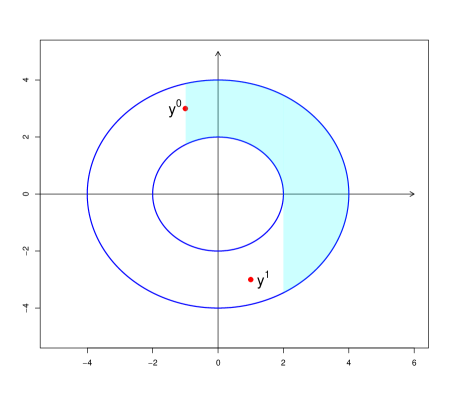
Figure 2: An illustration to Example 3.9. The boundaries of the annulus are blue. The shaded area are the points reachable under the state constraint $\mathcal{C}$.

We now introduce another reachability time. To start off, we define a solution satisfying the property that a small perturbation at any point does not break the reachability property. In the definition below we use the terms ‘reachability’ or ‘reachable’ with regard to system (1).

Definition 3.10.

Take $y^{0},y^{1}\in\mathcal{C}^{o}$, and let $z(t),h^{\perp}(t)$ be a solution of (6) with $z(0)=P_{H}y^{0}$, $z(T)=P_{H}y^{1}$. We call this solution pliable if

• $(i)$ for every $t_{1}$ and $t_{2}$, $0\leq t_{1}<t_{2}\leq T$, there exists $\varepsilon_{t_{1},t_{2}}>0$ and $\tau(t_{1},t_{2})>0$ with the property that for all $\varepsilon\leq\varepsilon_{t_{1},t_{2}}$ there is $\delta_{\varepsilon,t_{1},t_{2}}>0$ satisfying the following condition: for every $y_{t_{1}}\in\mathcal{B}(z(t_{1})+h^{\perp}(t_{1}),\delta_{\varepsilon,t_{1},t_{2}}){\cap\mathcal{C}^{\mathrm{o}}}$ there exists $y_{t_{2}}\in\mathcal{B}(z(t_{2})+h^{\perp}(t_{2}),\varepsilon){\cap\mathcal{C}^{\mathrm{o}}}$ such that $y_{t_{2}}$ is reachable from $y_{t_{1}}$ with state constraint $\mathcal{C}$ within the time $\tau(t_{1},t_{2})$ (that is, in a time not greater than $\tau(t_{1},t_{2})$).

• $(ii)$ For all $t\in[0,T]$ sufficiently close to $T$ there exists small $\delta_{t}>0$ such that $y^{1}$ is reachable from every point of $\mathcal{B}(z(t)+h^{\perp}(t),\delta_{t})$ with the state constraint $\mathcal{C}$, and

  $$\limsup\limits_{t\uparrow T}\sup\limits_{y\in\mathcal{B}(z(t)+h^{\perp}(t),\delta_{t}){\cap\mathcal{C}^{\mathrm{o}}}}T_{\mathcal{C}}(y,y^{1})=0.$$ (28)

• $(iii)$ The following inequality holds

  $$\limsup\limits_{\Delta t\to 0}\sup\limits_{t\in[0,T-\Delta t]}\frac{\tau(t,t+\Delta t)}{\Delta t}\leq 1.$$ (29)

While the definition of a pliable solution may seem unwieldy, intuitively it means that a solution to (6) can be approximate well by solutions to (1) along the entire trajectory without incurring significant loss of time.

Now we define

$$\begin{split}\widetilde{T}_{\mathcal{C}}(y^{0},y^{1})=\inf\big{\{}T:\text{there exists }z(t)\in C([0,T],H),h^{\perp}(t)\in L^{0}([0,T],H^{\perp})\text{ s.t. }z(0)=P_{H}y^{0},\\ z(T)=P_{H}y^{1},\text{ \eqref{system hat} holds and the solution is pliable}\big{\}}.\end{split}$$

The following result gives an upper bound of the reachability time $T_{\mathcal{C}}(y^{0},y^{1})$.

Proposition 3.11.

It holds that

$$T_{\mathcal{C}}(y^{0},y^{1})\leq\widetilde{T}_{\mathcal{C}}(y^{0},y^{1}).$$ (30)

Proof. Let $\varepsilon>0$ and let $z(t)\in C([0,T],H)$ and $h^{\perp}(t)\in L^{0}([0,T],H^{\perp})$ constitute a pliable solution to (6) with $z(0)=P_{H}y^{0}$, $z(T)=P_{H}y^{1}$, $T\leq\widetilde{T}_{\mathcal{C}}(y^{0},y^{1})+\varepsilon$. Take a partition $0=t_{0}<t_{1}<...<t_{k}<T$ such that

$$\sum\limits_{i=0}^{k-1}\tau(t_{i},t_{i+1})\leq T+\varepsilon,$$ (31)

and for some $\delta_{k}>0$

$$\sup\limits_{y\in\mathcal{B}(z(t_{k})+h^{\perp}(t_{k}),\delta_{k})}T_{\mathcal{C}}(y,y^{1})\leq\varepsilon.$$ (32)

We note that (31) and (32) are possible by items $(ii)$ and $(iii)$ of Definition 3.10, respectively. Next we define the sequence $r_{k},r_{k-1},...,r_{1}$ consecutively as follows: $r_{k}=\min(\delta_{k},\varepsilon_{t_{k-1},t_{k}})$, $r_{k-1}=\min(\delta_{r_{k},t_{k-1},t_{k}},\varepsilon_{t_{k-2},t_{k-1}})$, $r_{k-2}=\min(\delta_{r_{k-1},t_{k-2},t_{k-1}},\varepsilon_{t_{k-3},t_{k-2}})$ and so on, until $r_{1}=\min(\delta_{r_{2},t_{1},t_{2}},\varepsilon_{t_{0},t_{1}})$. It follows from Definition 3.10 that there is a solution $y(t)$ to (1) satisfying

$$y\left(\sum\limits_{i=0}^{j-1}\tau(t_{i},t_{i+1})\right)-(z(t_{j})+h^{\perp}(t_{j}))\leq r_{k},\ \ \ j=1,2,...,k-2,$$

and $y\left(\sum\limits_{i=0}^{k-1}\tau(t_{i},t_{i+1})\right)\in\mathcal{B}(z(t_{k})+h^{\perp}(t_{k}),\delta_{k})$. It follows from (32) that $y(t)$ can be extended to reach $y^{1}$ by the time $\sum\limits_{i=0}^{k-1}\tau(t_{i},t_{i+1})+\varepsilon$, that is, by the time $T+2\varepsilon$ if we take (31) into account. Since $\varepsilon>0$ is arbitrary, this completes the proof. ∎

Revisiting Example 3.8, we see by continuity of $F$ that the solution to (6) given there satisfies $(i)$ and $(iii)$ of Definition 3.10, but does not satisfy $(ii)$. Thus, if we modified $F$ near $y^{1}=(1,0,0)^{\top}$ in such a way that $(ii)$ of Definition 3.10 was satisfied, then by Proposition 3.11 we would have $T_{\mathcal{C}}(y^{0},y^{1})=2$.

In the next theorem we give a lower bound on the reachability time in the case $m<n-1$.

Theorem 3.12.

Let $m<n-1$. Denote $h_{k}=P_{H}y^{k}$, $k=0,1$. Denote also by $H_{\perp}$ the subspace of $H$ of co-dimension one such that $H_{\perp}\perp h_{1}-h_{0}$. Define

$$\bar{s}(h,h_{0},h_{1})=\frac{\max\langle F((h+H_{\perp}+H^{\perp})\cap\mathcal{C}),h_{1}-h_{0}\rangle}{|h_{1}-h_{0}|}.$$

Then

$$T_{\mathcal{C}}(y^{0},y^{1})\geq\int\limits_{h\in[h_{1},h_{2}]}\frac{dh}{\bar{s}(h,h_{0},h_{1})}.$$ (33)

Proof. Let $y(t)$, $t\in[0,T]$, be the a solution to (1) with constraint $y(t)\in\mathcal{C}$. Let $x(t)$ be the orthogonal projection of $y(t)$ on the line spanned by $h_{1}-h_{0}$. Then $x(0)=h_{0}$, $x(T)=h_{1}$, and

$$\dot{x}(t)\in F_{H}\left((x(t)+H_{\perp}+H^{\perp})\cap\mathcal{C}\right).$$

Hence

$$\begin{gathered}\frac{\langle\dot{x}(t),h_{1}-h_{0}\rangle}{|h_{1}-h_{0}|}\leq\sup\left\{\left\langle F_{H}\left((x(t)+H_{\perp}+H^{\perp})\cap\mathcal{C}\right),h_{1}-h_{0}\right\rangle\right\}\leq\bar{s}(x(t),h_{0},h_{1}).\end{gathered}$$

Since

$$\int\limits_{0}^{T}\frac{\langle\dot{x}(t),h_{1}-h_{0}\rangle}{|h_{1}-h_{0}|}dt=|h_{1}-h_{0}|,$$

the statement of the proposition follows from Lemma A1. ∎

Remark 3.13.

In the case $\overline{T}_{\mathcal{C}}(y^{0},y^{1})<\infty$, the signal $u(t)$ resulting in a time close to the infimum can be computed as follows: let $h\in[h_{0},h_{1}]$ be such that $P_{H}y(t)=h=h(t)$, $P_{H^{\perp}}y(t)=h^{\perp}=h^{\perp}(t)$ , $h\neq h_{0},h_{1}$. Then $u(t)$ is informally determined by $h,h^{\perp}$ from the system

$$\begin{cases}\sup\{\langle F_{H}\big{(}(h+H^{\perp})\cap\mathcal{C}\big{)},h_{1}-h_{0}\rangle\}=\langle F_{H}(h+h^{\perp}),h_{1}-h_{0}\rangle\\ h+h^{\perp}\in\mathcal{C},\\ \dot{h}+\dot{h}^{\perp}=F(h+h^{\perp})+Bu.\end{cases}$$ (34)

Note that the supremum in the first equation in (34) is not always achieved (for example, if $\mathcal{C}$ is open, the maximum need not be achieved). In this case, we may either consider the closure of $\mathcal{C}$, or replace $\sup\{\langle F_{H}\big{(}(h+H^{\perp})\cap\mathcal{C}\big{)},h_{1}-h_{0}\rangle\}$ with some $\sup\{\langle F_{H}\big{(}(h+H^{\perp})\cap\mathcal{C}\big{)},h_{1}-h_{0}\rangle\}-\delta$ for a small $\delta>0$.

After finding $u(t)$, we just set $y(t)=h(t)+Bu(t)$. We note that, typically, the infimum in (2) can not be achieved with an $L^{\infty}$ control, see [6] for the linear case. Most of the time system (34) would have a solution only if we allow the impulse control, i.e., we would allow $u$ to take value in some space of distribution. This is the approach taken in [7] for a linear system with a control constraint. In this way we could handle an instantaneous movement along a direction from $H^{\perp}$. To stay within $L^{\infty}$ controls, we may need to approximate the solution to (34) with $L^{\infty}$ controls. The approximation should be possible in most cases, however care needs to be taken to do the approximation properly, and it is impossible to do in certain situations as demonstrated by Example 3.8. The approximation is discussed in [7].

4 Examples

In this section we give three examples for which we compute the controllability time. In the next example we apply Theorem 3.7 to a three-dimensional control system.

Example 4.14.

Let $n=3$, $m=2$, $F(y)=Ay$,

$$\mathcal{C}=\left\{(x_{1},x_{2},x_{3})\mid x_{3}^{2}+\frac{x_{2}^{2}}{4}+\frac{x_{1}^{2}}{16}\leq 1\right\}.$$

$$A=(a_{ij})_{i,j=1,2,3}=\begin{pmatrix}-0.1&7.0&0\\ 0.0&0.8&7\\ 0.0&-10.0&-4\end{pmatrix},\ \ \ B=\begin{pmatrix}0&0\\ 1&2\\ 0&1\end{pmatrix},$$

and the initial and target state $y^{0}=(-1,0,0)^{T}$, $y^{1}=(1,0,0)^{T}$. In this example $H=\{(\kappa,0,0)^{T},\kappa\in\mathbb{R}\}$, and for $h\in[h_{0},h_{1}]$, $h=(\kappa,0,0)^{T}$, $\kappa\in[-1,1]$,

$$s(h,h_{0},h_{1})=\max\left\{a_{11}\kappa+a_{12}\beta+a_{13}\gamma:\frac{\kappa^{2}}{16}+\frac{\beta^{2}}{4}+\gamma^{2}\leq 1\right\}$$

$$=\max\left\{-0.1\kappa+7\beta:\frac{\beta^{2}}{4}\leq 1-\frac{\kappa^{2}}{16}\right\}=-0.1\kappa+14\sqrt{1-\frac{\kappa^{2}}{16}}.$$

Hence by Theorem 3.7

$$\begin{gathered}T_{\mathcal{C}}(y^{0},y^{1})=\int\limits_{h\in[h_{0},h_{1}]}\frac{dh}{s(h,h_{0},h_{1})}=\int\limits_{\kappa\in[-1,1]}\frac{d\kappa}{-0.1\kappa+14\sqrt{1-\frac{\kappa^{2}}{16}}}.\end{gathered}$$ (35)

$\Diamond$

In the next example some of the points are not reachable.

Example 4.15.

Let $n=2$, $m=1$, $\mathcal{C}$ be the square

$$\mathcal{C}=\{(x_{1},x_{2})\mid|x_{1}|\leq 1,|x_{2}|\leq 1\},$$

and let $F(y)=Ay$,

$$A=\begin{pmatrix}-2&3\\ -2&1\end{pmatrix},\ \ \ B=\begin{pmatrix}1\\ 1\end{pmatrix},$$ (36)

We have here $H=(\text{ran}(B))^{\perp}=\{(\kappa,-\kappa)^{\top}\mid\kappa\in\mathbb{R}\}$, and

$$P_{H}=\begin{pmatrix}0.5&-0.5\\ -0.5&0.5\end{pmatrix},\ \ \ A_{H}=P_{H}A=\begin{pmatrix}0&2\\ 0&-2\end{pmatrix}.$$ (37)

Take $y^{0}=(0.7,-0.5)^{\top}$, $y^{1}=(-0.5,0.3)^{\top}$. Then $h_{0}=(0.6,-0.6)^{\top}$, $h_{1}=(-0.4,0.4)^{\top}$. For $h=(\kappa,-\kappa)^{T}\in[h_{0},h_{1}]$, $\kappa\in[-0.4,0.6]$, we compute

$$s(h,h_{0},h_{1})=\frac{\max\{\langle A_{H}((h+H^{\perp})\cap\mathcal{C}),h_{1}-h_{0}\rangle\}}{|h_{1}-h_{0}|}=\frac{\max\{\langle A_{H}((h+H^{\perp})\cap\mathcal{C}),(-1,1)^{T}\rangle\}}{\sqrt{2}}$$

$$=\frac{1}{\sqrt{2}}\max\left\{\left\langle\begin{pmatrix}0&2\\ 0&-2\end{pmatrix}\begin{pmatrix}\kappa+\alpha\\ -\kappa+\alpha\end{pmatrix},\begin{pmatrix}-1\\ 1\end{pmatrix}\right\rangle\middle|\begin{pmatrix}\kappa+\alpha\\ -\kappa+\alpha\end{pmatrix}\in\mathcal{C}\right\}$$

$$=\sqrt{2}\max\Big{\{}2\kappa-2\alpha\Big{|}|\kappa+\alpha|\leq 1,|-\kappa+\alpha|\leq 1\Big{\}}=2\sqrt{2}(\kappa+1-|\kappa|),$$

where we used that the maximum is achieved for $\alpha=-1+|\kappa|$.

Thus, by Theorem 3.7

$$T_{\mathcal{C}}(y^{0},y^{1})=\frac{1}{2\sqrt{2}}\int\limits_{\kappa\in[-0.4,0.6]}\frac{d\kappa}{1+2\min(0,\kappa)}=\frac{1}{2\sqrt{2}}(0.6+\ln 5).$$

Now, in this example not every point within $\mathcal{C}$ is reachable from any other. Take for example $y^{2}=(-0.6,0.6)^{T}$, $h_{2}=y^{2}$. Then following the same steps as above, we find that for $h=(\kappa,-\kappa)^{T}\in[h_{0},h_{2}]$, $\kappa\in[-0.6,0.6]$

$$s(h,h_{0},h_{2})=2\sqrt{2}(\kappa+1-|\kappa|).$$

Thus, $s(h,h_{0},h_{2})<0$ for example for $h=(-0.55,0.55)^{T}$. Hence by Theorem 3.7, $T_{\mathcal{C}}(y^{0},y^{2})=\infty$, and $y^{2}$ is not reachable from $y^{0}$. This example is illustrated in Figure 3. $\Diamond$

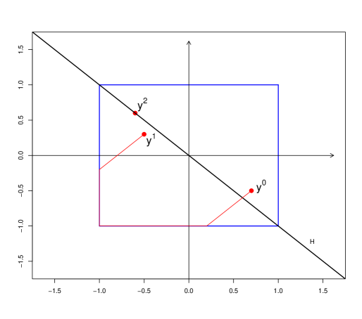
Figure 3: The optimal trajectory from $y^{0}$ to $y^{1}$ for (1) in Example 4.15. The boundaries of $\mathcal{C}$ are blue. The point $y^{2}$ is not reachable from $y^{0}$.

In the next example we deal with a non-linear system.

Example 4.16.

Let $n=2$, $m=1$,

$$\mathcal{C}=\{(x_{1},x_{2})\mid x_{1}^{2}+x_{2}^{2}\leq 5\},$$

and let

$$F(x)=\frac{1}{(10-x_{1})^{2}+(4-x_{2})^{2}}\frac{\left(10-x_{1},4-x_{2}\right)^{\top}}{|\left(10-x_{1},4-x_{2}\right)^{\top}|},$$

$B=\begin{pmatrix}0\\ 1\end{pmatrix}$, $y^{0}=(-4,-1)^{\top}$, $y^{1}=(4,-2)^{\top}$. Here $F$ represents attraction of a body located at $x=(x_{1},x_{2})^{\top}$ toward a source located at $\rm{S}=(10,4)^{\top}$ with the strength of attraction being reversely proportional to the square of the distance between $x$ and $\rm{S}$.

In this case $H=\{(\kappa,0)^{\top}\mid\kappa\in\mathbb{R}\}$, $h_{0}=(-4,0)^{\top}$, $h_{1}=(4,0)^{\top}$. We compute for $h=(\kappa,0)^{\top}$

$$s(h,h_{0},h_{1})=\begin{cases}\begin{aligned} &\frac{(10-\kappa)^{2}}{\big{(}(10-\kappa)^{2}+(4-\sqrt{25-\kappa^{2}})^{2}\big{)}^{2}},&-4\leq\kappa\leq 3\\ &\frac{1}{(10-\kappa)^{2}},&-3<\kappa<3,\\ &\frac{(10-\kappa)^{2}}{\big{(}(10-\kappa)^{2}+(4-\sqrt{25-\kappa^{2}})^{2}\big{)}^{2}},&3\leq\kappa\leq 4\end{aligned}\end{cases}$$ (38)

and hence by Theorem 3.7

$$T_{\mathcal{C}}(y^{0},y^{1})=\int\limits_{-4}^{-3}\frac{\big{(}(10-\kappa)^{2}+(4-\sqrt{25-\kappa^{2}})^{2}\big{)}^{2}}{(10-\kappa)^{2}}d\kappa+\int\limits_{-3}^{3}(10-\kappa)^{2}d\kappa+\int\limits_{3}^{4}\frac{\big{(}(10-\kappa)^{2}+(4-\sqrt{25-\kappa^{2}})^{2}\big{)}^{2}}{(10-\kappa)^{2}}d\kappa$$

$$\approx 182.9087+618+42.9122=843.8209.$$

This example is illustrated in Figure 4. $\Diamond$

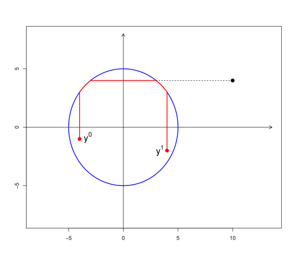
Figure 4: The optimal trajectory for Example 4.16. The source of attraction $\rm{S}$ is the big black dot on the right.

5 Conclusions and further comments

For a non-linear system with linear control and bounded convex state constraint we give results about the controllability time between two points. The results of [6] are extended in two directions: the system has a non-linear drift term, and the expression for the controllability time is valid in higher dimension. The main technique used in this paper consists in considering auxiliary systems obtained via orthogonal projection. Our results are exact in the case when the range of $B$ is of co-dimension one (Theorem 3.7). As shown in Example 3.8, the conclusions of Theorem 3.7 do not hold without the assumption $\dim H=1$.

We conclude with the following remarks about desirable extensions.

• In this paper we worked with a convex bounded constraint set. In our analysis we can replace the assumption that $\mathcal{C}$ is convex with the assumption that the projection of $\mathcal{C}$ on $H$ is convex. On the other hand, unbounded constraint sets require further considerations. We also expect the ideas developed here to be applicable to the case of a nice bounded constraint set with holes, for example an annulus.

• The case when $\dim H\geq 2$ is intriguing. Lemma 3.5 and Proposition 3.11 do shed some light on relation between equations (1) and (6), whereas Example 3.8 demonstrates pitfalls of trying to express $T_{\mathcal{C}}$ via $\overline{T}_{\mathcal{C}}$. Our intuitive guess is that Example 3.8 is rather contrived, and ‘in most cases’ the equality $T_{\mathcal{C}}=\overline{T}_{\mathcal{C}}$ should hold. This ‘in most cases’ could be formulated as certain parameters of the system being generic as in [6, Theorem 1] (that is, belonging to a dense open set), or, alternatively, as $T_{\mathcal{C}}=\overline{T}_{\mathcal{C}}$ holding with probability one when the parameters of the system are drawn from some continuous distributions.

Appendix

Here we formulate and prove a technical result used in Section 3. The next lemma is used to establish a lower bound for the time $T$ the system needs to travel a certain distance $M$.

Lemma A1.

Let $f$ be a non-negative differentiable function with $f(0)=0$, $\dot{f}(t)\leq g(f(t))$, and $f(T)=M$ for $T,M>0$ and a positive function $g$. Then $T\geq\int\limits_{0}^{M}\frac{dv}{g(v)}$, and the equality is achieved if $\dot{f}(t)=g(f(t))$.

Proof. Let $h$ be defined as the solution to

$$\dot{h}(t)=g(h(t)),\ \ \ {h(0)=0}.$$ (39)

By the comparison theorem, $f(t)\leq h(t)$, $t\geq 0$. It follows from (39) that $h$ is strictly increasing and thus inversible, and hence $\frac{dt}{d{h}}=\frac{1}{g(h)}$, $t=\int\limits_{0}^{h}\frac{dv}{g(v)}$. Hence for $T_{M}:=\int\limits_{0}^{M}\frac{dv}{g(v)}$ we get $h(T_{M})=M$. Thus, $f(T_{M})\leq h(T_{M})=M$, and therefore $f(T)=M$ implies $T\geq T_{M}=\int\limits_{0}^{M}\frac{dv}{g(v)}$. Finally, if $f=h$, then $T=T_{M}=\int\limits_{0}^{M}\frac{dv}{g(v)}$. ∎

References

BQRR [04]
Rainer Buckdahn, Marc Quincampoix, Catherine Rainer, and Aurel
Răşcanu.
Stochastic control with exit time and constraints, application to
small time attainability of sets.
Applied Mathematics and Optimization, 49(2):99–112, Apr 2004.
Hen [99]
Jeff Henrikson.
Completeness and total boundedness of the hausdorff metric.
MIT Undergraduate Journal of Mathematics, 1:69–80, 1999.
Hol [10]
Petr Holický.
Borel classes of uniformizations of sets with large sections.
Fund. Math., 207(2):145–160, 2010.
KB [07]
Sangho Ko and Robert R Bitmead.
State estimation for linear systems with state equality constraints.
Automatica, 43(8):1363–1368, 2007.
Kra [08]
Mikhail I Krastanov.
On the constrained small-time controllability of linear systems.
Automatica, 44(9):2370–2374, 2008.
LTZ [18]
Jérôme Lohéac, Emmanuel Trélat, and Enrique Zuazua.