FIRST CO-SPATIAL COMPARISON OF STELLAR, NEUTRAL-, AND IONIZED-GAS METALLICITIES IN A METAL-RICH GALAXY: M83¹¹1Based on observations made with the Hubble Space Telescope under program ID 14681.

Svea Hernandez AURA for ESA, Space Telescope Science Institute, 3700 San Martin Drive, Baltimore, MD 21218, USA Alessandra Aloisi Space Telescope Science Institute, 3700 San Martin Drive, Baltimore, MD 21218, USA Bethan L. James AURA for ESA, Space Telescope Science Institute, 3700 San Martin Drive, Baltimore, MD 21218, USA Nimisha Kumari AURA for ESA, Space Telescope Science Institute, 3700 San Martin Drive, Baltimore, MD 21218, USA Danielle Berg The Ohio State University, 4061 McPherson Chemical Laboratory, 140 W 18th Ave., Columbus, OH 43210 Angela Adamo Department of Astronomy, Oskar Klein Centre, Stockholm University, AlbaNova University Centre, SE-106 91 Stockholm, Sweden William P. Blair Department of Physics and Astronomy, The Johns Hopkins University, 3400 N. Charles Street, Baltimore, MD 21218 Claude-André Faucher-Giguère Department of Physics and Astronomy, Northwestern University, 2145 Sheridan Road, Evanston, IL 60208-3112 Andrew J. Fox AURA for ESA, Space Telescope Science Institute, 3700 San Martin Drive, Baltimore, MD 21218, USA Alexander B. Gurvich Department of Physics & Astronomy and CIERA, Northwestern University, 1800 Sherman Ave, Evanston, IL 60201, USA Zachary Hafen Department of Physics and Astronomy and Center for Interdisciplinary Exploration and Research in Astrophysics (CIERA), Northwestern University, 2145 Sheridan Road, Evanston, IL 60208, USA Timothy M. Heckman Center for Astrophysical Sciences, Department of Physics and Astronomy, The Johns Hopkins University, Baltimore, MD 21218, USA Vianney Lebouteiller AIM, CEA, CNRS, Université Paris-Saclay, Université Paris Diderot, Sorbonne Paris Cité, F-91191 Gif-sur-Yvette, France Knox S. Long Space Telescope Science Institute, 3700 San Martin Drive, Baltimore, MD 21218, USA Eureka Scientific, Inc. 2452 Delmer Street, Suite 100, Oakland, CA 94602-3017, USA Evan D. Skillman Minnesota Institute for Astrophysics, School of Physics and Astronomy, 116 Church Street S.E., University of Minnesota, Minneapolis, MN 55455, USA Jason Tumlinson Space Telescope Science Institute, 3700 San Martin Drive, Baltimore, MD 21218, USA Center for Astrophysical Sciences, Department of Physics and Astronomy, The Johns Hopkins University, Baltimore, MD 21218, USA Bradley C. Whitmore Space Telescope Science Institute, 3700 San Martin Drive, Baltimore, MD 21218, USA

Abstract

We carry out a comparative analysis of the metallicities from the stellar, neutral-gas, and ionized-gas components in the metal-rich spiral galaxy M83. We analyze spectroscopic observations taken with the Hubble Space Telescope (HST), the Large Binocular Telescope (LBT) and the Very Large Telescope (VLT). We detect a clear depletion of the H I gas, as observed from the H I column densities in the nuclear region of this spiral galaxy. We find column densities of log[ $N$ (H I) cm^-2] $<$ 20.0 at galactocentric distances of $<$ 0.18 kpc, in contrast to column densities of log[ $N$ (H I) cm^-2] $\sim$ 21.0 in the galactic disk, a trend observed in other nearby spiral galaxies. We measure a metallicity gradient of $-$ 0.03 $\pm$ 0.01 dex kpc^-1 for the ionized gas, comparable to the metallicity gradient of a local benchmark of 49 nearby star-forming galaxies of $-$ 0.026 $\pm$ 0.002 dex kpc^-1. Our co-spatial metallicity comparison of the multi-phase gas and stellar populations shows excellent agreement outside of the nucleus of the galaxy hinting at a scenario where the mixing of newly synthesized metals from the most massive stars in the star clusters takes longer than their lifetimes ( $\sim$ 10 Myr). Finally, our work shows that caution must be taken when studying the metallicity gradient of the neutral-gas component in star-forming galaxies, since this can be strongly biased, as these environments can be dominated by molecular gas. In these regions the typical metallicity tracers can provide inaccurate abundances as they may trace both the neutral- and molecular-gas components.

galaxies – abundances – ISM – starburst

^†^†journal: ApJ^†^†facilities: HST(COS)^†^†software: CLOUDY (Ferland et al., 2017), VoigtFit v.0.10.3.3 (Krogager, 2018), CALCOS pipeline (v.3.3.4)

1 Introduction

Understanding the formation and evolution of galaxies continues to be one of the main quests in modern astrophysics. Extragalactic abundance measurements have greatly contributed to uncover a variety of physical and evolutionary processes influencing events taking place within and among galaxies. Studies of galactic gradients and global metallicity relations (i.e., mass-metallicity relation, MZR) are widely used to investigate star-formation episodes, galactic winds, and accretion of pristine matter (Searle, 1971; McCall et al., 1985; Zaritsky et al., 1994; Tremonti et al., 2004; Andrews & Martini, 2013; Kudritzki et al., 2015).

The measurements from both the MZR and metallicity trends in star-forming galaxies (SFGs), have relied for decades on the analysis of emission lines from H II regions. Typically, when inferring the gas-phase metallicities from the most common heavy element, oxygen, two main techniques are applied: strong-line analysis, and the electron temperature based ( $T_{e}$ -based) method. The strong-line analysis is based on the flux ratios of some of the strongest forbidden lines, e.g., [O II] and [O III], with respect to hydrogen (Pagel et al., 1979; McGaugh, 1994). On the other hand, the “direct” method, or $T_{e}$ -based method, relies on the flux ratio of auroral to nebular lines, e.g., [O III] $\lambda$ 4363/[O III] $\lambda\lambda$ 4959, 5007, to measure the temperature of the high-excitation zone (Dinerstein et al., 1985; Rubin et al., 1994; Lee et al., 2004; Stasińska, 2005). Furthermore, in the last decades these nebular techniques have been extended to studies of star-forming galaxies at high redshift (Pettini et al., 2001; Kobulnicky & Kewley, 2004; Savaglio et al., 2005; Cowie & Barger, 2008). Although the analysis of H II regions have made invaluable contributions when it comes to investigating the present-day chemical state of starburst galaxies, these regions could be enhanced compared to the surrounding interstellar medium (ISM, Kunth & Sargent, 1986; Lebouteiller et al., 2013). And only in a few cases (e.g., Sánchez Almeida et al., 2015; Lagos et al., 2018) studies have found the metallicities in H II regions to be lower than the rest of the galaxy. This has been attributed to infall of cold metal-poor gas.

An alternative method for investigating the chemical composition of galaxies is to directly study the neutral gas in SFGs. The metal content of a galaxy can be examined through the analysis of the absorption lines in their far ultraviolet (UV) spectroscopic observations. A common technique is to use bright UV targets within these galaxies as background sources (Kunth et al., 1994). In such observations, the metals along the line of sight imprint absorption features on the UV continuum of such targets. This technique has been applied extensively to local galaxies (Aloisi et al., 2003; Lebouteiller et al., 2013; Werk et al., 2013; James et al., 2014). This approach not only allows us to study the metal contents accounting for the bulk of the mass of the galaxy, it also provides us with a view of the metal enrichment over large spatial scales and long timescales (dilution of abundances in H I regions).

A third approach to studying the metallicities of star-forming galaxies is the analysis of young stellar populations or individual stars. New techniques have been developed in the last decade to investigate the chemical contents of nearby galaxies using blue supergiants, BSGs, and red supergiants, RSGs, as metallicity tracers (Davies et al., 2010, 2015, 2017a, 2017b; Kudritzki et al., 2012, 2013, 2014; Hosek et al., 2014). Additionally, it is also possible to measure stellar metallicities from integrated-light spectroscopic observations of star clusters in nearby galaxies using high-resolution observations (Colucci et al., 2011, 2012; Larsen et al., 2006, 2008, 2012, 2014, 2017, 2018). This same technique has most recently been extended to intermediate-resolution observations of extragalactic stellar populations (Hernandez et al., 2017, 2018a, 2018b, 2019) as well as for populations at high redshifts (Halliday et al., 2008; Steidel et al., 2016; Chisholm et al., 2019).

In spite of the variety of tools available to investigate the chemical composition of star-forming galaxies, detailed comparisons of the abundances obtained from the ionized-gas, neutral-gas, and stellar components are needed to fully understand the chemical state and evolution of galaxies. The general expectation is that young populations of stars should have a similar chemical composition as their parent gas cloud and associated H II region. In this context, several studies in low-metallicity and chemically homogenous environments have shown agreement between the ionized-gas and young stellar population metallicities (Bresolin et al., 2006; Lee et al., 2006). Studies of different galaxies with higher metallicities, such as spiral galaxies, have shown a varying degree of agreement between their nebular and stellar metallicities, from excellent ( $<$ 0.1 dex) to differences as high as $\sim$ 0.2 dex (Bresolin et al., 2009, 2016; Hosek et al., 2014; Davies et al., 2017b). Even more intriguing is the fact that different studies have also hinted that for high-metallicity environments the T_e-based method underestimates the metallicities; this is suggested when compared to stellar abundances (Zurita & Bresolin, 2012; Simón-Díaz & Stasińska, 2011; García-Rojas et al., 2014). These high-metallicity environments are particularly challenging to study as the application of the direct method is limited given that the temperature-sensitive lines are typically too weak to be detected (Bresolin et al., 2005).

Studies comparing different metallicity diagnostics show conflicting results. Through a study of 30 SFGs at z $\sim$ 2, Steidel et al. (2016) found a factor of $\sim$ 4-5 difference between their inferred stellar and nebular metallicities, with a clear enhancement in the metallicities of the ionized gas. They argue that these artificially low stellar metallicities are observed due to the supersolar $\alpha$ /Fe abundance ratios of these galaxies at z $\sim$ 2. They assume that this behavior is expected at high redshift, and might be rare in low- $z$ environments due to systematic differences in the star-formation history of typical galaxies. In a more recent study, Chisholm et al. (2019) measure the metallicity of these same components, ionized-gas and stellar, in a sample of 61 SFGs at z $<$ 0.2, and 19 galaxies at z $\sim$ 2. In contrast to the work by Steidel et al. (2016), Chisholm et al. (2019) conclude that the stellar and nebular metallicities are similar to each other when assuming mixed-age stellar populations. Under the general assumption that young stellar populations have a similar chemical composition as their parent gas cloud and associated H II region, the work by Chisholm et al. (2019) hints at a scenario where the gas surrounding high-mass stars is not instantaneously metal-enriched by massive stars. This would imply that increasing the metallicity of the adjacent interstellar gas takes longer than the inferred lifetimes ( $\sim$ 10 Myr) of the massive stellar populations.

In this paper we analyze observations from the Cosmic Origin Spectrograph (COS) on Hubble, as well as data from the Multi-Object Double Spectrograph (MODS) on the Large Binocular Telescope (LBT) and the Multi Unit Spectroscopic Explorer (MUSE) on the Very Large Telescope (VLT) for a sample of pointings distributed across the face of the metal-rich spiral galaxy M83 (NGC 5236). M83 is our nearest face-on grand-design spiral and starburst galaxy (Dopita et al., 2010) at a distance of 4.9 Mpc (Jacobs et al., 2009, derived from the magnitudes of the tip of the red giant branch, TRGB). Its proximity and orientation allow for a spatially resolved study of its different components: stellar, neutral gas, and ionized gas. We present in Table 1 a detailed list of the general parameters of M83. Our main motivation is to understand how abundances from the different galaxy components relate to each other, particularly in a challenging environment as is the metal-rich regime. In Section 2 we describe the observations and data reduction. The analysis of the different observations and for the different metallicity components is detailed in Section 3. We discuss our findings in Section 4, and provide our concluding remarks in Section 5.

Table 1: General parameters for M83

Parameter	Value
R.A. (J2000.0)	204.253958^∘
Dec (J2000.0)	-29.865417^∘
Distance^a	4.9 Mpc
Morphological type	SAB(s)c
$R_{25}\>^{b}$	6.44 $\arcmin\;$ (9.18 kpc)
Inclination^b	24°
Position Angle^c	45°
Heliocentric radial velocity	512.95 km s^-1

Notes. All parameters from the NASA Extragalactic

Database (NED), except where noted.

^$a$Jacobs et al. (2009)

^$b$de Vaucouleurs et al. (1991)

^$c$Comte (1981)

2 Observations and Data Reduction

2.1 COS observations

The analysis done here relies on the observations taken as part of HST program ID (PID) 14681 (PI: Aloisi), collected between 2017 May–July. The targets were acquired using near-UV (NUV) imaging, and the spectroscopic data were observed with the G130M/1291 and G160M/1623 settings returning wavelength coverage from 1130 to 1800 Å. The data were collected at Lifetime Position 3 providing a wavelength-dependent resolution ranging between $R\sim$ 15,000 and 20,000. The targets observed in HST program ID 14681 were chosen from the list of young star clusters in the Wide Field Camera 3 (WFC3) Early Release Science Cycle 17 GO/DD PID 11360 (PI: O’Connell) and Cycle 19 GO PID 12513 (PI: Blair). An overview of this WFC3 multi-wavelength campaign is provided in Blair et al. (2014). Our selection criterion required targets to have magnitudes $m_{\rm F336W}\lesssim$ 17. We list in Table 2 the properties of our COS sample along with the information of their observations. We note that the spectroscopic observations for the M83-5 pointing were affected by a guide star filure after the science exposures began collecting data. This caused the S/N of the resulting spectroscopic data for this target to be lower than originally planned. For this reason we have excluded this target from our analysis.

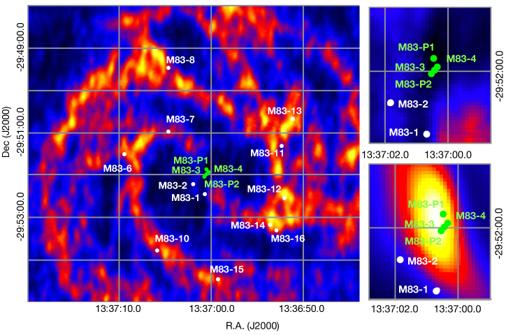
In addition to the targets from PID 14681, we extended our analysis to include two more COS pointings, M83-POS1 and M83-POS2, observed as part of HST PIDs 11579 and 15193 (PI: Aloisi). These additional observations were taken using the G130M/1291 and G160M/1623 setting with similar wavelength coverage as that from PID 14681. Our final COS sample is composed of 17 pointings distributed throughout the disk of M83 as indicated in Figure 1.

We retrieved the observations from the Mikulski Archive for Space Telescopes (MAST) and calibrated them using the HST pipeline, CALCOS v3.3.4 (Fox et al., 2015). More details on the reduction of the observations are provided by Hernandez et al. (2019). As a final step we bin the spectra by a COS resolution element (1 resel = 6 pixels), corresponding to the nominal point-spread function.

Refer to caption — Figure 1: $Left$ : Color-composite image observed with the 2.2m Max Planck-ESO Telescope, the 8.2m Subaru Telescope (NAOJ), and the Hubble Space Telescope. We marked with cyan circles the location of the star clusters observed with COS. We overlay the footprints of the MODS slits in red showing the position of the observed H II regions. MUSE FoV are shown in yellow. Processing and Copyright: Robert Gendler. $Right$ : Spitzer Local Volume Legacy Survey H $\alpha$ image of M83 (Dale et al., 2009). The footprint of the LBT/MODS mask is shown as a gray square, with sky slits (blue) and H II region slit locations (red) overlaid in comparison to the stellar clusters targeted with COS (cyan diamonds). The slit positions targeted H II regions associated with YMCs, although additional associated H II regions were added in order to maximize effective usage of mask real estate.

Table 2: Properties of the observed targets and their COS Observations

Cluster	R.A.^†	Dec^†	$m_{\rm F336W}^{a}$	$R/R_{25}$ ^b	$t_{\rm exp}$ (s)		S/N ^c (resel^-1)
	(^∘)	(^∘)	(mag)		G130M	G160M	G130M	G160M
M83-1	204.2527583	-29.8739111	17.00	0.08	2368	8114	1.5	1.3
M83-2	204.2576792	-29.8703833	16.14	0.06	2120	5652	2.2	1.5
M83-3	204.2517375	-29.8666222	15.10	0.02	400	1304	6.9	5.5
M83-4	204.2514333	-29.8662056	14.40	0.02	500	1208	3.1	2.2
M83-5	204.2504500	-29.8642500	14.85	0.04	1600	3072	0.9	0.6
M83-6	204.2895625	-29.8588083	16.46	0.34	1036	3645	4.0	3.5
M83-7	204.2692667	-29.8495917	14.79	0.21	540	1136	2.2	1.3
M83-8	204.2688667	-29.8246056	16.76	0.41	2987	7183	6.8	4.1
M83-9	204.2904083	-29.8187833	15.65	0.56	1056	3617	3.6	2.5
M83-10	204.2746000	-29.8959056	16.94	0.34	1780	5835	8.0	5.5
M83-11	204.2179875	-29.8557389	16.65	0.35	2092	5653	5.4	3.2
M83-12	204.2171125	-29.8764111	16.84	0.36	2892	7277	6.3	4.3
M83-13	204.2127208	-29.8444639	16.76	0.43	2232	5653	5.6	3.4
M83-14	204.2230583	-29.8863750	15.30	0.35	400	1296	2.8	1.7
M83-15	204.2465708	-29.9075222	16.24	0.40	1040	3644	2.1	1.6
M83-16	204.2204833	-29.8887472	16.79	0.38	2988	7169	5.4	3.4
M83-POS1	204.2519088	-29.8651611	16.15	0.02	4093	1240	20.7	3.3
M83-POS2	204.2521171	-29.8670056	15.52	0.02	2284	420	30.6	2.9

^$\dagger$Coordinates extracted from the Mikulski Archive at the Space Telescope Science Institute (MAST). We note that the HST performance has jitter of 0.008 $\arcsec\>$ RMS⁴⁴4https://hst-docs.stsci.edu/hsp.

^$a$Magnitudes are in the Vegamag system, calculated using a 2.5 $\arcsec\>$ aperture size.

^$b$Calculated adopting the parameters listed in Table 1.

^$c$Estimated at wavelengths of 1310 Å and 1700 Å for G130M and G160M, respectively.

2.2 MODS observations

Optical spectra of the H II regions in M83 were acquired with MODS (Pogge et al., 2010) on the LBT on the UT date of 2018 May 21. The primary goal was to obtain high signal-to-noise spectra, with detections of the intrinsically faint auroral lines (e.g., [O III] $\lambda$ 4363, [N II] $\lambda$ 5755, [S III] $\lambda$ 6312), in order to obtain accurate abundances of the gas surrounding the ionizing young massive clusters (YMCs) observed with COS and presented by Hernandez et al. (2019). To do so, we used the multi-object mode of MODS, which uses custom-designed, laser-milled slit masks, allowing multiple H II regions to be targeted simultaneously. We highlight that two masks were originally cut to cover the whole COS sample. However, due to poor weather conditions and other complications, only half of the data were collected. The M83 mask used, which targets 13 H II regions simultaneously, was observed for three exposures of 1200s, or a total integration time of 1-hour. At the latitude of the LBT, M83 stays below 30^∘ on the sky, and thus the observations were obtained at relatively high airmass ( $\sim$ 2–3). To compensate, slits were cut close to the median parallactic angle of the observing window (PA=0), minimizing flux lost due to differential atmospheric refraction between 3200 – 10,000 Å (Filippenko, 1982). Blue and red spectra were obtained simultaneously using the G400L (400 lines mm^-1, $R\sim 1850$ ) and G670L (250 lines mm^-1 $R\sim 2300$ ) gratings, respectively. The resulting combined spectra extend from 3200–10000 Å, with a resolution of $\sim 2$ Å(FWHM).

Broad R-band and continuum-subtracted H $\alpha$ images of M83 from The Spitzer Local Volume Legacy Survey (LVL; Dale et al., 2009) were used to identify the sample of target H II regions, as well as the alignment stars. H II regions were selected by prioritizing the knots of high H $\alpha$ surface brightness that are in the closest physical proximity to the YMCs. All target slits are 1.0″ wide, but with lengths varying according to the size of each H II region. The resulting multi-slit mask contained 13 H II region slits and 2 sky slits. We list in the Appendix in Table 9 the coordinates of each of the slits. The mask slit locations are shown in Figure 1 in comparison to the stellar clusters. Within the slit mask footprint, and avoiding aberration issues near the edges, we were able to target six distinct H II regions that directly correspond to YMC regions. To effectively use the mask real estate, we targeted six additional H II regions that do not clearly correspond to one the of YMCs (R4, R5, R9, R13, R14, and R15).

The M83 optical spectra were reduced and analyzed using the MODS reduction pipeline²²2 http://www.astronomy.ohio-state.edu/MODS/Software/modsIDL/ following the procedures detailed in Berg et al. (2015). Here, we summarize notable reduction steps. Given the crowding of bright H II regions in the disk of M83, diffuse nebular emission can complicate local sky subtraction. Therefore, the additional sky slits cut in the mask were used to provide a basis for clean sky subtraction. Continuum subtraction was performed in each slit by scaling the continuum flux from the sky-slit to the local background continuum level. One-dimensional spectra were then corrected for atmospheric extinction and flux calibrated based on observations of flux standard stars (Bohlin, 2014).

2.3 MUSE observations

To complement our COS and MODS observations we make use of archival MUSE data covering 12 out of 17 clusters in our COS sample with spectral resolution increasing between $R\sim$ 1770 at the bluest wavelengths (4800 Å) and $R\sim$ 3590 at the reddest wavelengths (9300 Å). The observations were taken during 2016 April and 2017 April–May as part of PID: 096.B-0057(A) with PI: Adamo. We downloaded the fully reduced datacubes from the European Southern Observatory (ESO) archive. The datacubes are reduced using the MUSE pipeline v.2.0.1, which performs removal of instrumental artifacts, astrometric calibration, sky-subtraction, wavelength and flux calibrations. We note that upon further inspection we found that the astrometric calibration for these archival datacubes was not correct, so we manually corrected their astrometry through a comparison with HST images.

We identify the location of the 12 clusters in our COS sample within the MUSE cubes and extract their spectra. The extraction was done by summing all spectra within circular apertures of diameter 2.5 $\arcsec$ co-spatial with the HST/COS pointings, taking into account the fractional level of overlap of the spatial pixel with the region. We identified a few bad pixels in the datacubes and excluded them from our analysis. In the left panel of Figure 1 we highlight in yellow the fields of view of MUSE.

3 Analysis

3.1 Neutral-gas Metallicities

3.1.1 Continuum and line-profile fitting

As part of the analysis performed we normalized the individual COS spectroscopic observations before fitting the different line profiles. We fit the continuum of the star clusters by interpolating between regions (nodes) strategically positioned to avoid stellar and ISM absorption. We make use of a spline function when interpolating between the manually defined nodes.

We derive the column densities for the different elements by fitting Voigt profiles using the recently developed Python software VoigtFit v.0.10.3.3 (Krogager, 2018). This relatively new code allows users to provide line spread function (LSF) tables to account for the broadening of the absorption lines introduced by the instrument itself. We convolve the COS LSF profiles with the FWHM of the source in the dispersion direction as measured from the acquisition images, similar to the approach described in Section 3.3 in Hernandez et al. (2020). We also note that VoigtFit allows for multi-component fitting, particularly useful for deblending different components along the same line of sight.

We note that although the COS observations allow us to access a variety of absorption lines of several heavy elements, our work focuses on measuring the metallicity of the neutral gas. Given that S/H traces metallicity reliably (Lebouteiller et al., 2013; James & Aloisi, 2018) we primarily study the S II and Ly $\alpha$ lines. We present in Table 3 the theoretical parameters for each of the lines analyzed as part of this work. We show in Figures 2 and 3 the best fitting profiles for the Lyman $\alpha$ and S II lines along with the COS observations.

Table 3: Atomic Data for UV absorption lines

Line ID	$\lambda_{\rm rest}$	$f^{a}$
	(Å)
Ly $\alpha$	1215.6710	4.16e-01
S II	1250.5780	5.43e-03
S II	1253.8050	1.09e-02

^$a$Oscillator strength values compiled by the Vienna Atomic

Line Database 3 (VALD3).

3.1.2 H I

The COS observations analyzed here cover the Ly $\alpha$ absorption line at $\lambda=$ 1215.671 Å originating from the multiple sightlines in M83. Given the close proximity of M83, the Ly $\alpha$ absorption from the MW is heavily blended with those from our M83 pointings. In order to extract precise column densities for the H I gas in M83 we simultaneously fit the MW and galaxy Ly $\alpha$ profiles. Following the approach adopted by James et al. (2014), we make use of the red wing of Ly $\alpha$ to constrain the fit of the H I column density intrinsic to the different targets, and adopt a fixed MW H I column density measured in James et al. (2014) in the direction of M83, $\log$ [ $N$ (H I)_MW cm^-2] = 20.57. Measurements of the H I column densities of the individual pointings in M83, $\log[$ $N$ (H I)], are listed in Table 4. Lastly, the best fitting profiles for the whole sample are shown in different panels in Figure 2.

3.1.3 S II

In general, direct measurements of the oxygen abundances in the neutral gas are difficult to access as the most easily observed O I line, 1302 Å, in the COS spectral coverage at low redshifts is typically saturated. On the other hand, O I at 1355 Å is too weak to be detected. As such, we use proxies for oxygen to indirectly derive the oxygen abundances (James & Aloisi, 2018). As part of our analysis we measure the column densities of the S II lines listed in Table 3 and make use of the solar ratio of $\log$ (S/O)_⊙ = $-$ 1.57 $\pm$ 0.06 to derive the O/H abundances in the neutral gas of M83.

3.1.4 Curve-of-growth Analysis

To assess if our measured abundances are affected by saturation, we plot the column density measurements along the curve-of-growth (COG) corresponding to the ion in question. For each ion we generate a COG showing the relation between the equivalent width, $\log$ ( $W/\lambda$ ), and the column density, $\log$ ( $fN$ ), where $f$ is the oscillator strength. When generating the individual COGs we adopt the $b$ parameters listed in Appendix B in Table 10 inferred from the simultaneous line-profile fitting of the S II lines.

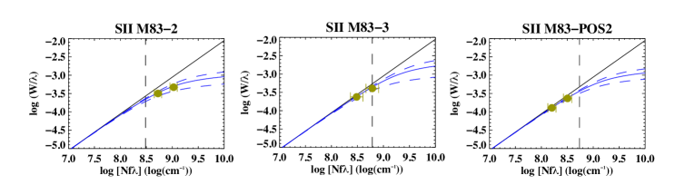
In Figure 4 we show a selected sample of COGs illustrating the line strength regimes encountered in our analysis. We primarily use the location of the S II transitions on their corresponding COG to determine if the column density estimates are reliable or if they need to be considered as lower limits due to saturation effects. For those pointings where both S II transitions are found on the right side of the vertical line, we consider them as saturated lines as they occupy the curved or saturated regime in the COG (see left panel in Figure 4). In those cases we are unable to constrain the column densities for S II and we consider them as lower limits. We also identified cases where one of the two transitions was found borderline or clearly in the saturated regime as shown in the middle panel of Figure 4. In such scenario we are still able to constrain the column densities as we fit the weakest transition, i.e., S II $\lambda$ 1250, avoiding hidden saturation effects. Lastly, we observed cases where both transitions were located on the linear part of the COG clearly showing an absence of saturation for those pointings.

Table 4: Column densities for the different pointings in M83.

Target	$\log$ [ $N$ (H I)]	$\log$ [ $N$ (S II)]	$\log$ [ $N$ (S II)]₂^a	$\log$ [ $N$ (S II)]_TOTAL	$\log$ [ $N$ (H I)]_ICF^b	$\log$ [ $N$ (S II)]_{TOTAL_ICF}^b
	(cm^-2)	(cm^-2)	(cm^-2)	(cm^-2)	(cm^-2)	(cm^-2)
M83-1	21.05 $\pm$ 0.08	15.99 $\pm$ 0.07^†	-	$>$ 15.99^†	21.17 $\pm$ 0.08	$>$ 16.09^†
M83-2	20.71 $\pm$ 0.08	15.89 $\pm$ 0.07^†	15.17 $\pm$ 0.11	$>$ 15.97^†	20.82 $\pm$ 0.08	$>$ 16.05^†
M83-3	18.99 $\pm$ 0.23	15.65 $\pm$ 0.12	-	15.65 $\pm$ 0.12	18.94 $\pm$ 0.23	15.25 $\pm$ 0.12
M83-4	19.56 $\pm$ 0.21	15.85 $\pm$ 0.08	-	15.85 $\pm$ 0.08	19.55 $\pm$ 0.21	15.68 $\pm$ 0.08
M83-5	21.01 $\pm$ 0.18	-	-	-	-	-
M83-6	20.60 $\pm$ 0.06	15.88 $\pm$ 0.07	-	15.88 $\pm$ 0.07	20.72 $\pm$ 0.06	15.96 $\pm$ 0.07
M83-7	20.65 $\pm$ 0.09	16.00 $\pm$ 0.05^†	15.38 $\pm$ 0.13	$>$ 16.09^†	20.65 $\pm$ 0.09	$>$ 16.06^†
M83-8	20.54 $\pm$ 0.03	15.79 $\pm$ 0.06	-	15.79 $\pm$ 0.06	20.65 $\pm$ 0.03	15.86 $\pm$ 0.06
M83-9	20.45 $\pm$ 0.07	15.70 $\pm$ 0.04	-	15.70 $\pm$ 0.04	20.56 $\pm$ 0.07	15.77 $\pm$ 0.04
M83-10	20.62 $\pm$ 0.02	15.88 $\pm$ 0.05^†	15.01 $\pm$ 0.22	$>$ 15.94^†	20.74 $\pm$ 0.02	$>$ 16.02^†
M83-11	20.05 $\pm$ 0.07	15.61 $\pm$ 0.04	-	15.61 $\pm$ 0.04	20.20 $\pm$ 0.07	15.68 $\pm$ 0.04
M83-12	20.85 $\pm$ 0.02	15.88 $\pm$ 0.03	-	15.88 $\pm$ 0.03	20.98 $\pm$ 0.02	15.97 $\pm$ 0.03
M83-13	20.63 $\pm$ 0.02	15.87 $\pm$ 0.05^†	-	$>$ 15.87^†	20.75 $\pm$ 0.02	$>$ 15.95^†
M83-14	20.43 $\pm$ 0.13	15.70 $\pm$ 0.05	14.96 $\pm$ 0.15	15.77 $\pm$ 0.05	20.43 $\pm$ 0.13	15.73 $\pm$ 0.05
M83-15	20.91 $\pm$ 0.05	15.81 $\pm$ 0.09	14.72 $\pm$ 0.47	15.84 $\pm$ 0.09	21.04 $\pm$ 0.05	15.94 $\pm$ 0.09
M83-16	21.05 $\pm$ 0.02	16.04 $\pm$ 0.04^†	-	$>$ 16.04^†	21.18 $\pm$ 0.02	$>$ 16.15^†
M83-POS1	19.93 $\pm$ 0.03	15.71 $\pm$ 0.06	15.02 $\pm$ 0.21	15.79 $\pm$ 0.06	19.92 $\pm$ 0.03	15.63 $\pm$ 0.06
M83-POS2	19.02 $\pm$ 0.03	15.37 $\pm$ 0.08	-	15.37 $\pm$ 0.08	18.91 $\pm$ 0.03	14.72 $\pm$ 0.08

^$a$Multi-component cases. A second S II component was identified for these pointings.

^$b$Column densities calculated after applying the ionization correction factors listed in Table 6.

^{^†}Column densities should be considered as lower limits.

3.1.5 Ionization corrections

In ISM abundance studies it is critical to take into account ionization effects due to contaminating ionized gas along the line of sight and/or contributing higher ionization ions present in the neutral gas, but not measured directly from the observations. Generating tailored photoionization models for a sample of nearby star-forming galaxies, Hernandez et al. (2020, hereafter H20) found ionization correction factors (ICFs) as high as $\sim$ 0.7 dex in the neutral gas, clearly demonstrating the importance of precise ICFs. To accurately infer the chemical abundances of the neutral gas along the different pointings throughout M83, as part of this work we investigate the amount of ionized gas contaminating the neutral abundance measurements (ICF_ionized), as well as the amount of higher ionization ions, compared to the dominant ion of a certain species in the H I gas (ICF_neutral).

To accurately estimate the ionization effects affecting our measured abundances we adopt a similar approach as that followed by H20. We generate tailored photoionization models for each of the pointings in our sample using the spectral synthesis code CLOUDY (Ferland et al., 2017). We adopt an overall metallicity of $Z$ = 3.24 $Z_{\odot}$ as measured from the ionized-gas component (Marble et al., 2010). The work of H20 takes advantage of newly acquired COS/FUV observations covering bluer wavelengths than our M83 COS/FUV data, which they use to measure the Fe III/Fe II ratio for the galaxies in their sample, including two M83 pointings in our analysis here (M83-POS1 and M83-POS2). This ratio is a critical indicator of the gas volume density of the targets and is essential to generate tailored photoionization models. Given that the Fe III line at $\lambda=$ 1122 $\rm\AA\;$ is not covered in our COS observations, we instead adopt an average value from the two M83 pointings in H20 of $\log$ [ $N$ (Fe III)/ $N$ (Fe II)] = $-$ 0.811 dex for the rest of the M83 targets studied here. Furthermore, H20 estimate the effective temperature of the star clusters observed in the two M83 pointings in their sample to be T ${}_{\rm eff}=$ 42,500 K. We adopt the same T_eff for the rest of our M83 pointings. We highlight that according to the work by H20, this physical parameter (T_eff) has minimal effects on the final ICF values calculated from the photoionization models. The rest of the input parameters are listed in Table 5. We estimate the log[L_UV] values from the $m_{\rm F336W}$ values listed in the Table 2, with the exception of M83-POS1 and M83-POS2; the log[L_UV] values for these two clusters were calculated using ACS/SBC frames observed with the F125LP filter. We measure the H I column densities directly from the COS observations as described in section 4.1. In the third column of Table 5 we show the measured volume densities using the assumed Fe III/Fe II ratios. For more details on the precise steps taken to generate the photoionzation models we refer the reader to Hernandez et al. (2020).

The different ICF values, ICF_ionized, ICF_neutral, and ICF_TOTAL, for the full M83 sample are listed on Table 6. Similar to the work of James et al. (2014) and H20 we calculate the final column densities for each element X using the following equation:

\log[N(X)_{\rm ICF}]=\log[N(X)]-\rm ICF_{\rm TOTAL}

(1)

In Table 6 we list the individual correction values, both ICF_ionized and ICF_neutral, for each ion and target. In the last two columns of Table 6 we show the total ionization correction factors to be applied to the measured column densities. And finally, we list in the last columns of Table 4 the ionization corrected column densities for H and S obtained after applying the inferred ICF_TOTAL using Equation 1.

Table 5: Input parameters for the CLOUDY models tailored to each of the M83 pointings in our sample

Target	$\log$ [L_UV]^a	log[ $n$ (H)]
	(erg s^-1)	(cm^-3)
M83-1	38.25	1.14
M83-2	38.60	2.31
M83-3	39.01	3.85
M83-4	39.30	3.97
M83-5	39.12	2.53
M83-6	38.48	2.29
M83-7	39.14	3.06
M83-8	38.36	2.22
M83-9	38.80	2.86
M83-10	38.28	2.00
M83-11	38.40	2.72
M83-12	38.32	1.70
M83-13	38.36	2.09
M83-14	38.94	3.05
M83-15	38.56	1.93
M83-16	38.34	1.20
M83-POS1	40.94^b	4.68^c
M83-POS2	41.40^b	5.72^c

^$a$Luminosities estimated from the $m_{\rm F336W}$ listed in Table 2.

^$b$Luminosities estimated from the ACS/SBC frames

observed with the F125LP filter (Hernandez et al., 2020).

^$c$Volume densities from Hernandez et al. (2020).

Table 6: Ionization Correction Factors for the M83 COS pointings

Target	H I	S II	H II	S III	H	S
	ICF_ionized		ICF_neutral		ICF_TOTAL
M83-1	0.00	0.00	0.12	0.10	$-$ 0.12	$-$ 0.10
M83-2	0.00	0.00	0.12	0.08	$-$ 0.12	$-$ 0.08
M83-3	0.08	0.40	0.04	0.01	0.04	0.40
M83-4	0.02	0.17	0.01	0.00	0.01	0.17
M83-5	0.00	0.00	0.12	0.10	$-$ 0.12	$-$ 0.10
M83-6	0.00	0.00	0.12	0.08	$-$ 0.12	$-$ 0.08
M83-7	0.00	0.03	0.00	0.00	$-$ 0.00	0.03
M83-8	0.00	0.00	0.12	0.08	$-$ 0.12	$-$ 0.08
M83-9	0.00	0.00	0.11	0.07	$-$ 0.11	$-$ 0.07
M83-10	0.00	0.00	0.12	0.08	$-$ 0.12	$-$ 0.08
M83-11	0.00	0.00	0.15	0.07	$-$ 0.15	$-$ 0.07
M83-12	0.01	0.00	0.12	0.10	$-$ 0.12	$-$ 0.10
M83-13	0.00	0.00	0.12	0.08	$-$ 0.12	$-$ 0.08
M83-14	0.00	0.04	0.01	0.00	$-$ 0.00	0.04
M83-15	0.00	0.00	0.12	0.10	$-$ 0.12	$-$ 0.10
M83-16	0.00	0.00	0.13	0.11	$-$ 0.13	$-$ 0.11
M83-POS1	0.02	0.16	0.01	0.00	0.01	0.15
M83-POS2	0.27	0.67	0.17	0.02	0.11	0.65

3.2 Nebular Metallicities

We measure the emission line fluxes from the optical observations (LBT and VLT) for the recombination and collisionally excited lines by fitting Gaussian profiles after subtracting the continuum and absorption features in the spectral region of interest. Equal weight is given to the flux in each spectral pixel while fitting the Gaussian profiles. We further propagate the uncertainties on the three Gaussian parameters (amplitude, centroid, and FWHM) to estimate the final uncertainty in the fluxes.

We use the attenuation curve by Fitzpatrick et al. (2019) along with the observed H $\alpha$ /H $\beta$ ratio to estimate the nebular emission line color excess, E(B-V), at an electron temperature and density of 10,000 K and 100 cm^-3, respectively (Case B recombination). We note that we have also tested our metallicity calculations assuming Case B recombination coefficients associated with an electron temperature of 5000 K (which may be more representative of the high metallicity gas within M83), and find that the final metallicity estimates are insensitive to the electron temperature adopted for the Case B recombination coefficient, within the uncertainties. The E(B-V) is then used to deredden the observed emission line fluxes. We include in Appendix C the tables listing the individual fluxes, dereddened fluxes and reddening values for each of the pointings studied here.

As part of our analysis we tested various diagnostics for estimating the gas-phase metallicities, which included R₂₃³³3([O II] $\lambda$ 3727+[O III] $\lambda\lambda$ 4959, 5007)/H $\beta$ , O3N2⁴⁴4([O III] $\lambda$ 5007/H $\beta$ )/([N II] $\lambda$ 6584/H $\alpha$ ), and N2⁵⁵5[N II] $\lambda$ 6584/H $\alpha$ (Pettini & Pagel, 2004; Curti et al., 2017). We note that the Curti et al. (2017) metallicity calibrations are only valid for 12+ $\log$ (O/H) $<$ 8.85, objects with metallicities of 12+ $\log$ (O/H) $=$ 8.85 need to be considered lower limits. This limitation drastically reduced the number of available metallicity measurements in our study, as we are primarily exploring a high-metallicity environment. In a previous metallicity study of M83 by Bresolin et al. (2016), they find that empirically calibrated strong-line diagnostics usually provide lower abundances than those inferred from the stellar populations. They attribute this behavior to the difficulties in selecting adequate samples when calibrating high metallicity environments. They note that among those strong-line methods tested in their work, the O3N2 calibration by Pettini & Pagel (2004) provides nebular abundances that are in best agreement with their BSG metallicities. For the rest of our study we adopt the O3N2 calibration by Pettini & Pagel (2004) as recommended by Bresolin et al. (2016). The uncertainties in the final nebular metallicities listed in the last two columns of Table 7 account for both the statistical and systematic components. We highlight that pointings M83-1 and M83-6 have been observed with both LBT and VLT. The metallicities calculated from these two sets of observations agree within their uncertainties.

Lastly, we performed a detailed inspection on possible contamination on our nebular fluxes due to nearby supernova remnants (SNRs). Using the catalogs by Blair et al. (2014), Blair et al. (2012), Dopita et al. (2010) and Russell et al. (2020) of previously identified SNRs in M83, we confirm that almost all of the slits and apertures are free of contamination, with the exception of LBT target R7 (see Table 9). We exclude this target from the rest of our analysis.

3.3 Stellar Metallicities

Hernandez et al. (2019) performed the first metallicity study of M83 using the integrated UV light of most of the YMCs we study here. More precisely they measure the metallicities of those targets observed in HST PID 14681. Hernandez et al. (2019) did not include the last two targets listed in Table 2 from HST PID: 11579 and 15193, M83-POS1 and M83-POS2. They applied the same full spectral fitting technique developed by Larsen et al. (2012), and previously applied to spectroscopic observations of stellar populations in the optical and NIR wavelength regime. Briefly summarized, this technique combines the information from the Hertzsprung-Russell diagram, stellar atmospheric models and synthetic spectra to derive abundances from the integrated light of single stellar populations.

In order to have stellar metallicities of our full M83 sample, we apply the same approach as that described in Hernandez et al. (2019) to measure the overall metallicities of the two missing clusters, M83-POS1 and M83-POS2. After some inspection of the individual targets and their acquisition images, we discovered that the 2.5″ COS aperture for M83-POS2 encompassed more than one YMC. Given that the COS observations for this target contained multiple stellar population, we were unable to estimate the stellar metallicity for this pointing as the analysis technique by Larsen et al. (2012) is optimized for single stellar populations.

We adopt an age of 3 Myr (Wofford et al., 2011) when fitting for the stellar metallicity of M83-POS1, and measure an overall metallicity of [Z] = $\log$ Z/Z_⊙ = $+$ 0.18 $\pm$ 0.12 dex. We adopt the solar oxygen abundance by Asplund et al. (2009), 12+ $\log$ (O/H) = 8.69, and obtain an oxygen abundance of 12+ $\log$ (O/H) = 8.87 for M83-POS1.

We list the final metallicities from all three components in Table 7.

Table 7: M83 metallicities of the stellar, neutral-gas, ionized-gas components for the COS pointings.

Target	12+log(O/H)_stellar	12+log(O/H)_neutral	12+log(O/H)_ionized	12+log(O/H)_ionized
	HST/COS	HST/COS	VLT/MUSE	LBT/MODS
			O3N2	O3N2
M83-1	9.26 $\pm$ 0.10	$>$ 8.48^†	8.80 $\pm$ 0.15	8.97 $\pm$ 0.14
M83-2	8.55 $\pm$ 0.17	$>$ 8.80^†	–	–
M83-3	9.02 $\pm$ 0.15	9.88 $\pm$ 0.27	8.85 $\pm$ 0.15	–
M83-4	8.71 $\pm$ 0.16	9.70 $\pm$ 0.23	8.86 $\pm$ 0.14	–
M83-5	–	–	–	–
M83-6	8.74 $\pm$ 0.12	8.81 $\pm$ 0.11	8.86 $\pm$ 0.20	9.00 $\pm$ 0.16
M83-7	8.90 $\pm$ 0.18	$>$ 8.99^†	–	–
M83-8	8.65 $\pm$ 0.14	8.78 $\pm$ 0.09	–	8.93 $\pm$ 0.14
M83-9	8.35 $\pm$ 0.08	8.77 $\pm$ 0.10	–	8.64 $\pm$ 0.14
M83-10	8.89 $\pm$ 0.15	$>$ 8.85^†	8.84 $\pm$ 0.14	–
M83-11	8.66 $\pm$ 0.09	9.05 $\pm$ 0.10	–	–
M83-12	8.81 $\pm$ 0.14	8.57 $\pm$ 0.07	8.84 $\pm$ 0.15	–
M83-13	8.75 $\pm$ 0.13	$>$ 8.77^†	–	–
M83-14	8.81 $\pm$ 0.19	8.87 $\pm$ 0.15	8.89 $\pm$ 0.14	–
M83-15	8.62 $\pm$ 0.08	8.47 $\pm$ 0.12	–	–
M83-16	8.87 $\pm$ 0.14	$>$ 8.53^†	8.86 $\pm$ 0.14	–
M83-POS1	8.87 $\pm$ 0.12	9.28 $\pm$ 0.09	9.00 $\pm$ 0.14	–
M83-POS2	–	9.38 $\pm$ 0.10	8.89 $\pm$ 0.14	–

^{^†}Metallicities should be considered as lower limits.

4 Discussion

4.1 H I distribution

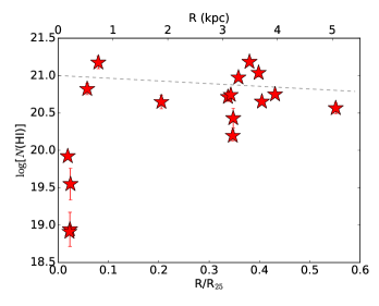
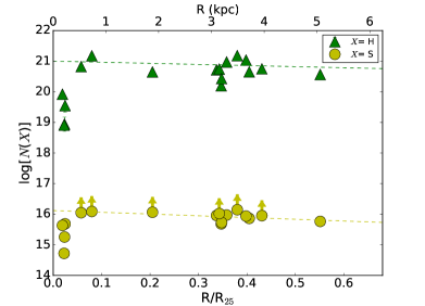
We show in Figure 5 the H I column density as a function of galactocentric distance, normalized to isophotal radius (see Table 1). We find a depletion of H I gas in the nuclear region of M83, with column densities of $\log$ [ $N$ (H I) cm^-2] $<$ 20.0. Our data indicate a general trend where at galactocentric distances R/R ${}_{\rm 25}>$ 0.02 the column density of H I increases to values of the order of $\log$ [ $N$ (H I) cm^-2] $\sim$ 21.0, typical of the disks of spiral galaxies (Kamphuis & Briggs, 1992; Bigiel et al., 2008; Ianjamasimanana et al., 2018), with a relatively flat gradient to larger galactocentric distances of $-$ 0.4 $\pm$ 1.1 dex $R_{\rm 25}^{-1}$ (dashed line in Figure 5).

Lundgren et al. (2004) found that the CO emission in M83, which is assumed to be linearly proportional to the mass surface density intensity of the molecular hydrogen (H₂), and the H I column density follow each other tightly with one clear exception at the nucleus, where they observed a clear depletion of H I. The low column densities reported in our study in the center of M83 clearly agree with the molecular- and neutral-gas maps in Lundgren et al. (2004).

To further investigate this anti-correlation between H I and molecular gas at the center of M83 we inspected the integrated 21-cm H I map observed and calibrated as part of The H I Nearby Galaxy Survey⁶⁶6http://www.mpia.de/THINGS/Overview.html (THINGS, Walter et al., 2008). In Figure 6 we show a map of the atomic hydrogen from THINGS using the Very Large Array (VLA) and a synthesized beam of 10.4″ $\times$ 5.6″. The archival image was made with natural weighting of the visibilities. In the top right image of Figure 6 we show a zoomed-in version of the nuclear region of M83. We mark with green circles the location of the four M83 pointings with $\log$ [ $N$ (H I) cm^-2] $<$ 20.0. We also show with white dots two pointings with $\log$ [ $N$ (H I) cm^-2] $>$ 20.0. From the H I map it is clear that a depletion of neutral hydrogen is present in the center of this spiral galaxy.

We contrast these results with the CO observations obtained with the Atacama Large Millimeter/submillimeter Array (ALMA) with an extremely high beam resolution of 2.03″ $\times$ 1.15″and published by Hirota et al. (2018). We obtained the calibrated CO map resulting after applying a mask to discard velocity pixels dominated by noise (kindly provided by A. Hirota). However, in order to perform a direct comparison with the lower-resolution H I map, we convolve the high-resolution CO map with a kernel created using the Gaussian profiles from both maps, H I and CO. As a last step we place the CO image in the same pixel scale as that from the H I map. The final CO map is shown in the lower right panel in Figure 6. Similar to the zoomed frame of the H I map, we also show in this CO image the location of the COS pointings with low column densities of H I with green dots. We confirm the strong contrast between the depletion of atomic hydrogen gas, and the excess of molecular gas at the core of M83.

Neutral atomic hydrogen has been observed to be depleted within the inner regions of many spiral galaxies (Morris & Lo, 1978; Sage & Solomon, 1991; Crosthwaite et al., 2000; Crosthwaite & Turner, 2007), however, the precise reason for this depletion is not completely understood. The most natural explanation would be the conversion of atomic gas to molecular gas in regions with high metallicities and dust contents. Since molecular gas is the primary driver of star-formation, star-forming regions are known to have higher molecular gas content (Kumari et al., 2020), naturally explaining the depletion in atomic gas in the center of M83. Moreover, given that H₂ molecules are created on the surface of dust, one crucial parameter regulating the formation of H₂ is the amount of dust, which is assumed to be proportional to the metallicity (Honma et al., 1995). This trend is clear in the work of Casasola et al. (2017), where they find a high concentration of dust in the core of M83, along with a depletion of H I in these same regions. Considering that in the nucleus of M83 we find the highest metallicities (see Section 4.2), a scenario where H I is converted to H₂ is the most reasonable explanation for the strong depletion observed in our H I column densities. Lastly, the column densities of $\log$ [ $N$ (H I) cm^-2] $\sim$ 21.0 observed just outside of the nuclear region of M83 correspond to the usual threshold where local galaxies begin to experience the H I–H₂ transition (Schaye, 2001; Krumholz et al., 2009a, b).

In the MW similar H I voids have been observed in the inner Galaxy (Lockman, 1984; Lockman & McClure-Griffiths, 2016). It has been proposed that the lack of H I in the central regions of the MW, compared to the rest of the Galactic disk, might hint at an excavation by Galactic winds (Bregman, 1980; Lockman & McClure-Griffiths, 2016). In addition to the scenario provided above, a second explanation for the depletion of H I observed in the center of M83 could be the excavation by galactic winds, as observed in the MW. This scenario would be supported by studies confirming the existence of an ongoing starburst in the center of this spiral galaxy (Dopita et al., 2010; Wofford et al., 2011) causing high cluster formation efficiencies (from about $\sim$ 26% in the inner region to 8% outside of this region) and a significant steepening of the initial cluster mass function in the inner regions of M83 (Adamo et al., 2015). The stellar feedback from these young massive star clusters in the core of M83 can generate energetic winds capable of ejecting large fractions of the neutral gas. Furthermore, through the analysis of high-resolution hydrodynamical simulations of the multiphase components of galactic winds, Schneider & Robertson (2017) find that momentum does not transfer efficiently, and therefore the momentum in the galactic winds is unable to accelerate the dense phase to the wind velocity, failing to entrain the cool dense gas. Until recently, the results from Schneider & Robertson (2017) were supported by the lack of evidence of cold dense molecular gas in the Galactic nuclear wind. Although this same process could possibly explain the excess in molecular gas observed in the nuclear regions of M83, a recent study by Di Teodoro et al. (2020) reports for the first time on the detection of molecular gas outflowing from the center of the MW. Di Teodoro et al. (2020) confirm that their results pose a challenge for current theoretical models of galactic winds in regular SFGs, as no process is currently able to explain the existence of fast-moving molecular gas in the MW nuclear wind.

4.2 Metallicity gradients in the multi-phase gas and stellar component

The discovery of the inhomogeneity of metals in the ISM throughout the MW (Shaver et al., 1983) has become a fundamental concept in our understanding of galaxy interactions, accretion, mergers and gas flows. Studies of nearby spiral galaxies have shown relatively higher metallicities in the inner regions compared to the outer disk, with gradients typically of the order of $\sim-$ 0.05 dex kpc^-1 (Pilkington et al., 2012). Most of the studies investigating metallicity gradients in local galaxies have focused on their ionized-gas component (H II regions, e.g., Walsh & Roy, 1997; Bresolin et al., 2005; Bresolin, 2007; Kewley et al., 2010; Ho et al., 2015; Bresolin, 2019; Kreckel et al., 2019), and to a lesser degree on the stellar component (Mollá et al., 1999; Carrera et al., 2008; Sánchez-Blázquez et al., 2011; Davies et al., 2017a). In contrast, metallicity gradients imprinted in the neutral gas of nearby galaxies have been rather unexplored.

In this section we will describe in detail the different metallicity trends presented in Figure 7 as inferred from the neutral gas (top left), ionized gas (top right), and stellar populations (lower left) in M83.

Assuming a single gradient (one without breaks), we also show in Figure 7 linear regressions for the different metallicity components. As previously discussed, given the high metallicities in the core of the galaxy, particularly in the neutral gas, we find a steep gradient of the order of $-$ 1.6 $\pm$ 0.4 dex $R_{\rm 25}^{-1}$ (dashed yellow line in upper left panel). We estimate a slightly shallower gradient for the stellar component of $-$ 1.0 $\pm$ 0.3 dex $R_{\rm 25}^{-1}$ (dotted-dashed red line in lower left panel), and a much shallower one for the ionized-gas component of $-$ 0.2 $\pm$ 0.1 dex $R_{\rm 25}^{-1}$ (dashed blue line in upper right panel). We note that to obtain an accurate view of the metallicity gradients, we exclude the lower limit values when fitting the neutral-gas measurements.

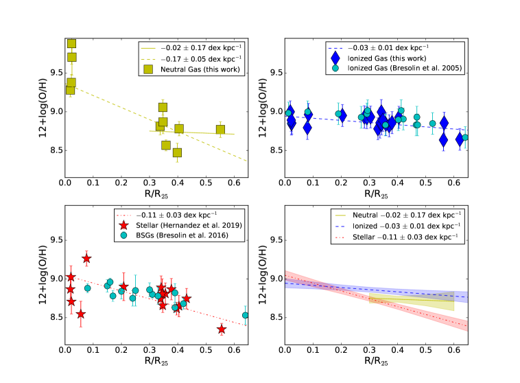
4.2.1 Neutral-gas metallicity gradient

The steep gradient observed in the neutral gas (upper left panel in Figure 7, $-$ 1.6 $\pm$ 0.4 dex $R_{\rm 25}^{-1}$ or $-$ 0.17 $\pm$ 0.05 dex kpc^-1) appears to be primarily driven by the low column densities of H I in the nucleus of the galaxy (discussed in Section 4.1). In an effort to better understand the derived neutral-gas metallicities in the core of M83 we display the column densities of H and S as a function of galactocentric distance in Figure 8. Figure 8 shows that the neutral metals, traced by S, are depleted at the center, to a lesser degree than H. To help guide the eye we apply linear regressions to the column densities of H and S at R/R ${}_{\rm 25}>0.02$ excluding the highly depleted pointings, and including the lower limits in S to have a better galactocentric coverage. We note that the inclusion of the lower limits in S returns a gradient which should be considered as a lower limit as well.

Following the trends in Figure 8, shown as dashed lines, and assuming the radial profile of H should hold in the center of M83, we would expect column densities of H of the order of $\log$ [ $N$ (H) cm^-2] $\sim$ 21.0, and instead we measure $\log$ [ $N$ (H) cm^-2] $\sim$ 18.9. This implies that $\sim 99\%$ of the neutral H has been depleted. Using S as a metallicity tracer in the neutral gas, from Figure 8 we would expect column densities of $\log$ [ $N$ (S) cm^-2] $\gtrsim$ 16.2, and instead measure column densities as low as $\log$ [ $N$ (S) cm^-2] $\sim$ 14.7. Note that for S, we basically assume that the S/H ratio is approximately constant. The observed trend hints at a depletion in the neutral metals of $\gtrsim 97\%$ . One possible explanation for the differences observed in the fraction of depleted neutral H and S might be linked to the high concentration of molecular gas in the nucleus of M83 discussed in Section 4.1.

Given that the medium in the center of this spiral galaxy is mainly in molecular form (Casasola et al., 2017), it is possible that a significant fraction of the measured S might be tracing the CO-dark H₂ gas, providing a biased estimate of the metals in the neutral gas. In the neutral gas, ions such as C⁺, Si⁺ and O⁰ can exist in both the H I and H₂ phases, particularly in regions where CO is photodissociated and molecular hydrogen is self-shielded (and shielded by dust) from UV photodissociation, typically called CO-dark H₂ gas (Madden et al., 1997; Wolfire et al., 2010). Since the ionization potential of S⁺ is comparable to that of C⁺, Si⁺ and O⁰, we might also expect S⁺ to coexist in the CO-dark H₂ phase. In such a scenario, and based on the calculations presented above, we estimate that from the measured column density of $\log$ [ $N$ (S) cm^-2] $\sim$ 14.7 and assuming a similar fraction of S and H, i.e., 99 $\%$ depletion, we can then infer that the column density of S arising from the CO-dark H₂ phase is of the order of $\log$ [ $N$ (S) cm^-2] $\sim$ 14.6. If this hypothesis proves to be accurate, we are possibly probing an intercloud or clumpy medium, where the matter is in the molecular (CO-dark) but diffuse phase. If we assume an efficient conversion from H I to H₂, we can expect a column density for the molecular hydrogen of the order of $\log$ [ $N$ (H₂) cm^-2] $\sim$ 21. We contrast this expected column density of H₂, with those observed from high-resolution CO maps (with a synthesized beam of 2.0 $\arcsec$ $\times$ 1.1 $\arcsec$ in full width at half maximum) by Egusa et al. (2018) where at the peak of the emission they observe column densities of the order of $\log$ [ $N$ (H₂) cm^-2] $\gtrsim$ 22, and between the peaks values of $\log$ [ $N$ (H₂) cm^-2] $\sim$ 20-21. We note that these column densities of H₂ are obtained assuming the Galactic conversion factor ( $X_{\rm CO}$ ) by Dame et al. (2001). These values would suggest that the medium in the center of M83 could be $\sim$ 10 $\%$ CO-dark H₂ gas towards the peaks observed in the CO maps, and 100 $\%$ CO-dark H₂ gas between the peaks. This hypothesis could be put to test by probing H₂ in absorption, which should trace both phases, the CO-dark and CO-bright. Finally, if such a high fraction of our inferred S column densities originates from the CO-dark H₂ gas, we may assume that in active and star-forming environments dominated by molecular gas, the typical neutral-gas metallicity tracers (e.g., S and O) provide a biased view of the total metal contents in the neutral ISM.

Regarding the neutral-gas trend, to confirm if indeed there is a gradient present outside the nuclear region of M83, we analyze the gradient of the neutral gas excluding those pointings in the nuclear region. We find instead a relatively flatter neutral-gas metallicity gradient of $-$ 0.02 $\pm$ 0.17 dex kpc^-1 (shown as solid yellow line in the upper right panel in Figure 7). Although we provide a value for a possible gradient in the neutral gas, outside of the nucleus of M83, we note that our measurement is limited by a low number of pointings available, primarily clustered around R $\sim$ 0.4 R₂₅. A larger sample, spanning a much broader galactocentric range, will be needed to reduce the uncertainties in our measurements allowing us to draw firmer conclusions and better characterize the metallicity gradient of the neutral gas.

Overall, our work shows that caution must be taken when studying the abundance gradients of spiral galaxies, as the intense activity in the center of these star-forming galaxies (outflows, high star-formation rates, high concentrations of molecular gas) can strongly bias the inferred neutral-gas gradients.

4.2.2 Ionized-gas metallicity gradient

In the upper right panel in Figure 7 we show with blue diamonds our inferred ionized-gas metallicities and with a blue dashed line the corresponding metallicity gradient, $-$ 0.3 $\pm$ 0.1 dex $R_{\rm 25}^{-1}$ or $-$ 0.03 $\pm$ 0.01 dex kpc^-1. We find an excellent agreement between our inferred abundances and those calculated by Bresolin et al. (2016) using the O3N2 calibration by Pettini & Pagel (2004) and the line fluxes from Bresolin et al. (2005), shown as cyan circles. Bresolin et al. (2016) calculate an ionized-gas metallicity gradient of $-$ 0.24 $\pm$ 0.06 dex $R_{\rm 25}^{-1}$ , similar to that measured here.

It is known that ionized-gas metallicity gradients in local galaxies are correlated with Hubble type, particularly bar strength and merging episodes. Studies have shown that relatively flatter gradients are found for barred galaxies and merging pairs than other types (Kewley et al., 2010; Rupke et al., 2010a). In a recent study by Ho et al. (2015), they inferred metallicity gradients from H II regions in 49 local star-forming galaxies and find a strong correlation between their stellar mass and the observed gradients. They provide a local benchmark of metallicity gradients where galaxies with stellar masses of log( $M_{*}/M_{\odot}$ ) $>$ 9.6 are expected to have gradients of the order of $-$ 0.026 $\pm$ 0.002 dex kpc^-1, in agreement with the median slope inferred for an isolated spiral control sample by Rupke et al. (2010b). M83 has a stellar mass of log( $M_{*}/M_{\odot}$ ) $=$ 10.55 (Bresolin et al., 2016) and, based on our analysis, an ionized-gas metallicity gradient of $-$ 0.03 $\pm$ 0.01 dex kpc^-1, well within the range of the masses defined by Ho et al. (2015) and with a gradient comparable to their benchmark value. The common slopes between the sample in Ho et al. (2015) and M83 imply that, in general, disk galaxies evolve in a similar manner when developing their disks, possibly following an inside-out disk growth model (Sánchez et al., 2014).

4.2.3 Stellar metallicity gradient

Hernandez et al. (2019) estimate a stellar metallicity gradient for M83 of $-$ 0.38 $\pm$ 0.20 dex $R_{\rm 25}^{-1}$ , the main difference between their study and the work presented here is the galactocentric ranges considered. Hernandez et al. (2019) examine the stellar metallicities at $R/R_{\rm 25}<$ 0.5, excluding the low metallicity cluster at $R/R_{\rm 25}\sim$ 0.55, whereas in this work we include all of the pointings when calculating the stellar gradient. The main driver for excluding the stellar cluster at $R/R_{\rm 25}$ $\sim$ 0.55 is justified by a proposed break in the abundance gradient (Hernandez et al., 2019). Given that such a break is less visible in the nebular metallicities calculated as part of this work, we decide to include this stellar cluster at $R/R_{\rm 25}$ $\sim$ 0.55 in our analysis.

In the lower left panel of Figure 7 we compare the stellar metallicities from our YMC sample (red stars) with those from the BSG sample (cyan circles) by Bresolin et al. (2016). To accurately compare the results from the two studies, we homogenize the inferred metallicities to a single abundance scale using equation 6 in Hernandez et al. (2019). We highlight the clear agreement between the two independent studies.

In the stellar metallicity study by Bresolin et al. (2016), they compare their measurements with those from the ionized gas using different strong-line indicators. In general, Bresolin et al. (2016) find that the H II abundance gradients are significantly shallower than those from the blue supergiants or those obtained from the direct T_e-method. In spite of the shallower gradient obtained using the O3N2 calibration, they suggest that the radial metallicity distribution and the scatter in their stellar abundances resemble those observed in the H II abundances inferred with O3N2 diagnostic. This pattern is similar to what we see in the work presented here, where the stellar metallicity gradient is slightly steeper (lower left panel in Figure 7) than that inferred for the ionized gas (upper right panel in Figure 7) using the O3N2 calibration.

In addition to observing a similar trend to that in Bresolin et al. (2016) when comparing our ionized-gas gradient with the stellar metallicity gradient, we also highlight the agreement between our inferred values. Bresolin et al. (2016) measure an abundance gradient of $-$ 0.66 $\pm$ 0.13 dex $R_{25}^{-1}$ using BSGs, and $-$ 0.81 $\pm$ 0.57 dex $R_{25}^{-1}$ from H II regions using the T_e-based method, well within the uncertainties of our stellar metallicity gradient, $-$ 1.0 $\pm$ 0.3 dex $R_{\rm 25}^{-1}$ .

4.2.4 Comparison of Global Metallicity Gradients

Lastly, in the lower right panel in Figure 7 we compare the metallicity gradients from the three different components: neutral-gas (solid yellow line), ionized-gas (dashed blue line), and stellar (dotted dashed red line). Overall, our work proves to be consistent with previous studies where metallicity gradients inferred from stellar populations are steeper than those measured in the ionized gas using strong-line calibrators. Furthermore, comparing the observed gradient for the stellar populations ( $-$ 0.11 $\pm$ 0.03 dex kpc^-1) in M83 to the benchmark gradient for nearby SFGs by Ho et al. (2015), we find that the stellar value is much higher than what is expected from the ionized-gas component, $-$ 0.026 $\pm$ 0.002 dex kpc^-1. On the other hand, the benchmark gradient and that inferred from the neutral-gas component, $-$ 0.02 $\pm$ 0.17 dex kcp^-1, agree within the large uncertainties of the inferred neutral-gas metallicity gradient.

Our work shows that it is critical to examine in detail the effects and activity in the nuclear regions of star-forming galaxies when studying metallicity gradients imprinted in the neutral-gas component, as these might be strongly biased if the dominant phase is molecular. And finally, we highlight that even when the inferred gradients for the different components appear to be dissimilar, we note that outside of the central regions the abundances of the multiphase gas and stellar populations appear to be more homogenized, with similar metallicities (within the uncertainties of our measurements) throughout the different components, e.g., at R $>$ 0.2 R₂₅. We discuss the metallicities of the individual pointings and their different components in the following section.

4.3 Co-spatial comparisons: Stellar, Neutral- and Ionized-gas Metallicities

We now compare the metallicities of the multi-phase ISM with those from the stellar populations for each individual COS pointing. This provides a co-spatial comparison on the small galactic scales of the star clusters ( $\sim$ 100 pc).

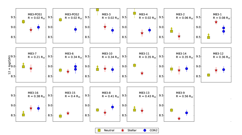
In Figure 9, we display individual panels comparing the metallicities of each phase, neutral-gas (yellow squares), stellar (red stars), and ionized-gas (blue diamonds). We can see that with the exception of two pointings, M83-1 and M83-9, the stellar metallicities and the nebular metallicities agree within their uncertainties. We note the contrast between these two pointings, M83-1 is close to the nuclear region of M83, and M83-9 is the pointing at the largest galactocentric distances in our sample. In general, the clear agreement we observed in our study supports a scenario where the gas surrounding these young populations of stars (average age $\sim$ 7 Myr), particularly the hot gas, is not instantaneously enriched by the most massive stars. We arrive at a similar conclusion to that in Chisholm et al. (2019), where the agreement between the abundances of the stellar populations and the ionized gas in a SFG sample at low ( $<$ 0.2) and high ( $\sim$ 2) redshifts indicate that the gas adjacent to the young stars is enriched at longer timescales than the lifetimes of the most massive stars. Our work shows that at least on small galactic scales of $\sim$ 100 pc it takes $>$ 10⁷ yr to fully mix the newly processed metals from the massive stars into the ISM. These longer than expected timescales imply caution must be taken when assuming instantaneous recycling approximations when generating galactic chemical evolution models (Kobulnicky & Skillman, 1997).

We find a similar trend for the neutral gas. The metallicities inferred for the neutral-gas component of M83 also show an overall agreement with those from both the stellar, and the ionized-gas component, once we accurately consider the lower limits. The exception to this general trend is found primarily in the nucleus of M83. We find that particularly at the core of M83, the metallicity of the neutral gas is more enhanced than that for the stellar and ionized-gas components. This is clearly seen in the first four top panels in Figure 9, M83-POS1, M83-POS2, M83-3 and M83-4. This enhancement in the metallicity of the neutral gas is discussed above in Section 4.2. Given that in the center of M83 the dominant phase is clearly molecular (Figure 6), the S column densities observed in these four pointings trace both the neutral and (CO-dark) molecular gas, providing a biased view of the neutral-gas metallicities.

Lastly, to further investigate a possible spatial difference between the neutral gas and the stellar populations, we look at the radial velocities of the neutral-gas and stellar components listed in Table 8. We find that the average radial velocity difference between the neutral gas and the stars is $\Delta\bar{v}$ = $v_{\rm neutral}-v_{\rm stellar}$ = $-$ 13.0 km s^-1 with a standard deviation of $\sigma$ = 34.4 km s^-1. For pointings M83-3 and M83-4 we find a radial velocity difference of $\Delta v$ = $-$ 42.9 km s^-1 and $-$ 40.4 km s^-1, respectively, within the standard deviation of the mean $\Delta\bar{v}$ in our sample. For M83-POS1, we estimate a larger velocity difference between the two components of $\Delta v$ = $-$ 65.1 km s^-1, potentially indicating that the neutral gas along the line of sight of M83-POS1 is occupying a spatially different region than that of the star cluster.

Overall, our co-spatial comparison shows that the three different components, neutral gas, ionized gas, and stellar populations, are chemically homogeneous on small scales ( $\sim$ 100 pc), with the exception of the nuclear region in M83. In the galactic center we are unable to make a direct comparison between the metallicity of the neutral gas and that of the ionized gas and stellar populations, as the inferred neutral-gas abundances are strongly biased due to the dominant molecular phase in these regions.

Table 8: Radial velocities for the neutral-gas and stellar component.

Target	$v_{\rm neutral}$	$v_{\rm stellar}^{a}$
	(km s^-1)	(km s^-1)
M83-1	497 $\pm$ 13	468 $\pm$ 43
M83-2	517 $\pm$ 9	503 $\pm$ 8
M83-3	465 $\pm$ 13	508 $\pm$ 9
M83-4	490 $\pm$ 15	530 $\pm$ 3
M83-5	–	–
M83-6	447 $\pm$ 9	443 $\pm$ 7
M83-7	477 $\pm$ 7	455 $\pm$ 17
M83-8	381 $\pm$ 15	464 $\pm$ 12
M83-9	442 $\pm$ 12	407 $\pm$ 22
M83-10	504 $\pm$ 14	514 $\pm$ 1
M83-11	513 $\pm$ 8	524 $\pm$ 22
M83-12	562 $\pm$ 7	539 $\pm$ 13
M83-13	523 $\pm$ 9	517 $\pm$ 1
M83-14	512 $\pm$ 8	560 $\pm$ 15
M83-15	538 $\pm$ 20	570 $\pm$ 4
M83-16	530 $\pm$ 6	539 $\pm$ 4
M83-POS1	430 $\pm$ 20	495 $\pm$ 10
M83-POS2	493 $\pm$ 19	–

^$a$Taken from Hernandez et al. (2019).

5 Conclusion

The work presented here aims at providing a comparative study of the multi-phase gas and the stellar component in the nearby spiral galaxy M83. We analyze HST/COS, LBT/MODS, and VLT/MUSE observations to estimate the metallicities of the neutral gas, ionized gas and stellar populations throughout the disk of this metal-rich galaxy. We summarize our results as follows:

1.

We find a clear depletion of H I gas as observed from the H I column densities in the core of M83. At galactocentric distances of R/R₂₅ $<$ 0.02 (R $<$ 0.18 kpc) we estimate column densities of the order of log[ $N$ (H I) cm^-2] $<$ 20.0. At galactocentric distances of R/R₂₅ $>$ 0.02 we find that the H I column densities increase to values of log[ $N$ (H I) cm^-2] $\sim$ 21.0, typical of spiral galaxies.
2.

After comparing the H I and molecular gas maps, we find a clear anti-correlation at the core of M83 where the region with depleted H I column densities shows a significant excess of molecular gas.
3.

Using the O3N2 calibration by Pettini & Pagel (2004) we measure a metallicity gradient of $-$ 0.03 $\pm$ 0.01 dex kpc^-1 for the ionized gas, comparable to the local benchmark of metallicity gradients of nearby star-forming galaxies by Ho et al. (2015), implying that disk galaxies evolve in a similar manner, following an inside-out model.
4.

Our work shows that outside of the nuclear region of M83 the metallicity of the neutral-gas, ionized-gas and stellar populations are comparable (within the uncertainties of our measurements) and more homogenized than in the nucleus of the galaxy. These findings call for caution when studying abundance gradients, particularly for the neutral-gas component, which can be strongly biased by the observed metallicities in the center as these are greatly affected by the efficient conversion from atomic to molecular gas.
5.

We find a slightly steeper stellar metallicity gradient, $-$ 0.11 $\pm$ 0.03 dex kpc^-1, compared to that observed in the ionized gas, $-$ 0.03 $\pm$ 0.01 dex kpc^-1, using the strong-line calibration of O3N2. This trend is similar to that observed in previous studies, where the abundance gradients inferred from strong-line calibrations are shallower than those observed from stellar populations.
6.

A co-spatial comparison of the metallicities of the multi-phase gas and the stellar populations show excellent agreement outside of the nucleus of the galaxy. This hints at a scenario where on small galactic scales ( $\sim$ 100 pc) it takes longer than the lifetime of the most massive stars ( $\sim$ 10 Myr) to fully mix the newly synthesized metals.

Overall, we observe homogeneous metallicities in the multi-phase gas and stellar component on small scales similar to those of stellar clusters in the high-metallicity environment of M83. Studies similar to that detailed in this paper are critical for validating this trend in a variety of other environments in the Local Universe. Lastly, we highlight that studies like the one presented here would benefit greatly from multiphase high spatial resolution simulations to further understand the feedback mechanisms and processes taking place as well as mixing timescales in much more detail.

These data are associated with the HST GO programs 14681, 11579, and 15193 (PI: A. Aloisi). Support for this program was provided by NASA through grants from the Space Telescope Science Institute. Some of the data presented in this paper were obtained from the Mikulski Archive at the Space Telescope Science Institute (MAST). This paper uses data taken with the MODS spectrographs built with funding from NSF grant AST-9987045 and the NSF Telescope System Instrumentation Program (TSIP), with additional funds from the Ohio Board of Regents and the Ohio State University Office of Research. This paper made use of the modsIDL spectral data reduction pipeline developed by Kevin V Croxall in part with funds provided by NSF Grant AST-1108693. This work was based in part on observations made with the Large Binocular Telescope (LBT). The LBT is an international collaboration among institutions in the United States, Italy, and Germany. The LBT Corporation partners are: the University of Arizona on behalf of the Arizona university system; the Istituto Nazionale di Astrofisica, Italy; the LBT Beteiligungsgesellschaft, Germany, representing the Max Planck Society, the Astrophysical Institute Potsdam, and Heidelberg University; the Ohio State University; and the Research Corporation, on behalf of the University of Notre Dame, the University of Minnesota, and the University of Virginia. CAFG was additionally supported by NSF through grants AST-1715216 and CAREER award AST-1652522; by NASA through grant 17-ATP17-0067; and by a Cottrell Scholar Award from the Research Corporation for Science Advancement. This work made use of THINGS, ‘The H I Nearby Galaxy Survey’.

Appendix A Observed LBT/MODS targets

We present the coordinates of the MODS pointings observed as part of PID: LBT-2018A- I0037-0 (PI: Skillman and Berg), and analyzed as part of our work. In Table 9 we list the coordinates of the MODS slits.

Table 9: LBT/MODS slit coordinates

Target	R.A.	Dec
	(^∘)	(^∘)
R1 (M83-9)	204.2917833	$-$ 29.8183306
R2 (M83-8)	204.2702875	$-$ 29.8247167
R3	204.3253625	$-$ 29.8080694
R4	204.2265583	$-$ 29.8412944
R5	204.2821417	$-$ 29.8543528
R6 (M83-6)	204.2900583	$-$ 29.8586167
R7	204.2508208	$-$ 29.8640583
R8 (M83-1)	204.2527333	$-$ 29.8754000
R9	204.2849000	$-$ 29.8696306
R10	204.3261792	$-$ 29.8812833
R11	204.2286583	$-$ 29.8860306
R12	204.2693667	$-$ 29.8498333
R13	204.2330833	$-$ 29.8316361
R14	204.2240375	$-$ 29.8126472
R15	204.2445000	$-$ 29.7994694

Appendix B Doppler $b$ parameter

As part of the neutral-gas analysis done on the COS observations, the VoigtFit software estimates the Doppler parameter, $b$ . In Table 10 we list the Doppler $b$ values obtained for the different M83 pointings. We do not include the Doppler parameter, $b$ , for the H I fits, as the line is in the damped part of the COG (James et al., 2014).

Table 10:

b

parameters for the M83 pointings.

Target	S II	S II₂^a
	(km s^-1)	(km s^-1)
M83-1	105.73 $\pm$ 21.55	–
M83-2	68.27 $\pm$ 9.85	101.30 $\pm$ 28.27
M83-3	139.74 $\pm$ 41.58	–
M83-4	124.33 $\pm$ 20.23	–
M83-5	–	–
M83-6	123.84 $\pm$ 31.97	–
M83-7	79.81 $\pm$ 16.72	53.94 $\pm$ 74.77
M83-8	109.62 $\pm$ 19.52	–
M83-9	163.28 $\pm$ 17.07	–
M83-10	118.69 $\pm$ 11.92	29.30 $\pm$ 23.59
M83-11	96.67 $\pm$ 7.49	–
M83-12	116.61 $\pm$ 8.88	–
M83-13	91.19 $\pm$ 10.63	–
M83-14	85.17 $\pm$ 11.70	54.29 $\pm$ 17.56
M83-15	111.33 $\pm$ 26.15	14.33 $\pm$ 38.41
M83-16	105.28 $\pm$ 11.02	–
M83-POS1	127.29 $\pm$ 15.56	88.73 $\pm$ 39.19
M83-POS2	127.21 $\pm$ 28.32	–

^$a$Multi-component cases. A second S II component was identified for these pointings.

Appendix C Optical emission line fluxes

We present tables detailing the individual emission line measurements for both the LBT/MODS (Tables 11–12) and VLT/MUSE observations (Tables 13–14).

\movetabledown

=2.2in {rotatetable}

Table 11: Emission line measurements (relative to H

\beta

= 100) for the LBT spectra. Line fluxes (F_λ) are extinction corrected using E(B-V) to calculate I_λ.

Target	$[OII]$		$H\beta$		$[OIII]$		$[NII]$		$H\alpha$
	(3726.03 Å)		(4861.33 Å)		(5006.84 Å)		(6548.03 Å)		(6562.80 Å)
	F_λ	I_λ	F_λ	I_λ	F_λ	I_λ	F_λ	I_λ	F_λ	I_λ
R1	$139.25\pm 35.64$	$188.66\pm 54.43$	$100.00\pm 3.45$	$100.00\pm 8.06$	$67.73\pm 3.05$	$64.56\pm 10.05$	$43.39\pm 4.19$	$30.73\pm 3.49$	$404.77\pm 15.61$	$286.00\pm 28.42$
R2	$86.23\pm 4.70$	$130.84\pm 25.07$	$100.00\pm 2.68$	$100.00\pm 12.97$	$9.23\pm 0.67$	$8.64\pm 1.38$	$54.26\pm 6.02$	$33.79\pm 6.38$	$460.77\pm 16.04$	$286.00\pm 45.77$
R3	–	–	–	–	–	–	–	–	–
R4	$73.17\pm 1.72$	$113.85\pm 12.22$	$100.00\pm 0.69$	$100.00\pm 6.37$	$27.55\pm 0.52$	$25.70\pm 2.47$	$59.35\pm 5.58$	$35.92\pm 4.65$	$474.20\pm 10.27$	$286.00\pm 25.14$
R5	$66.09\pm 5.48$	$100.46\pm 19.04$	$100.00\pm 3.62$	$100.00\pm 13.51$	$8.95\pm 0.84$	$8.38\pm 1.87$	$54.61\pm 6.71$	$33.95\pm 6.80$	$461.68\pm 20.13$	$286.00\pm 49.63$
R6	$100.67\pm 9.06$	$120.61\pm 29.51$	$100.00\pm 3.85$	$100.00\pm 13.22$	$5.22\pm 2.84$	$5.08\pm 2.83$	$40.94\pm 4.43$	$33.34\pm 6.09$	$351.64\pm 15.37$	$286.00\pm 44.19$
R7	$30.31\pm 6.85$	$71.36\pm 15.66$	$100.00\pm 0.94$	$100.00\pm 4.00$	$10.19\pm 0.39$	$8.90\pm 0.57$	$4121.12\pm 4.80$	$45.81\pm 2.85$	$761.52\pm 10.60$	$286.00\pm 13.49$
R8	$41.20\pm 7.59$	$79.13\pm 19.14$	$100.00\pm 2.21$	$100.00\pm 12.24$	$7.61\pm 1.04$	$6.86\pm 1.24$	$78.39\pm 7.08$	$37.36\pm 6.15$	$603.37\pm 17.91$	$286.00\pm 39.63$
R9	$63.45\pm 5.39$	$137.20\pm 22.16$	$100.00\pm 2.43$	$100.00\pm 8.51$	$11.64\pm 0.85$	$10.31\pm 1.38$	$93.73\pm 3.87$	$39.04\pm 3.87$	$690.95\pm 17.63$	$286.00\pm 27.73$
R10	–	–	–	–	–	–	–	–	–
R11	$57.80\pm 19.29$	$77.15\pm 23.81$	$100.00\pm 2.10$	$100.00\pm 8.30$	$8.59\pm 0.55$	$8.21\pm 0.84$	$47.81\pm 2.43$	$34.44\pm 3.49$	$397.99\pm 9.19$	$286.00\pm 25.85$
R12	$49.35\pm 5.31$	. $59.42\pm 9.71$	$100.00\pm 3.20$	$100.00\pm 8.68$	$5.30\pm 0.55$	$5.14\pm 0.69$	$30.37\pm 4.70$	$24.60\pm 4.32$	$353.68\pm 14.04$	$286.00\pm 31.73$
R13	$80.49\pm 4.08$	$93.88\pm 13.98$	$100.00\pm 1.20$	$100.00\pm 9.16$	$18.07\pm 0.67$	$17.64\pm 2.29$	$37.29\pm 4.66$	$31.31\pm 4.43$	$341.02\pm 9.18$	$286.00\pm 28.90$
R14	$115.59\pm 2.50$	$151.47\pm 17.87$	$100.00\pm 1.29$	$100.00\pm 6.85$	$17.54\pm 0.49$	$16.81\pm 1.50$	$52.78\pm 4.80$	$38.83\pm 5.06$	$389.60\pm 9.62$	$286.00\pm 25.53$
R15	$134.84\pm 1.45$	$205.98\pm 12.85$	$100.00\pm 0.59$	$100.00\pm 4.98$	$73.52\pm 0.93$	$68.78\pm 4.40$	$55.61\pm 3.39$	$34.38\pm 3.15$	$464.31\pm 6.50$	$286.00\pm 16.62$

\movetabledown

=2.2in {rotatetable}

Table 12: Emission line measurements (relative to H

\beta

= 100) for the LBT spectra. Line fluxes (F_λ) are extinction corrected using E(B-V) to calculate I_λ.

Target	$[NII]$		$[SII]$		$[SII]$		$E(B-V)$	F( $H\beta$ )
	(6583.41 Å)		(6716.47 Å)		(6730.85 Å)
	F_λ	I_λ	F_λ	I_λ	F_λ	I_λ		F_λ	I_λ
R1	$133.09\pm 6.30$	$93.71\pm 10.58$	$51.77\pm 2.20$	$35.66\pm 4.00$	$36.12\pm 1.79$	$24.82\pm 2.58$	$0.324\pm 0.029$	$4.99\pm 0.17$	$15.07\pm 1.21$
R2	$166.45\pm 7.90$	$102.82\pm 16.15$	$48.07\pm 1.99$	$28.81\pm 4.17$	$34.50\pm 1.77$	$20.61\pm 3.17$	$0.446\pm 0.033$	$24.56\pm 0.66$	$111.73\pm 14.49$
R3	–	–	–	–	–	–	–	–
R4	$176.06\pm 6.35$	$105.65\pm 9.31$	$43.66\pm 1.43$	$25.37\pm 2.41$	$31.81\pm 1.42$	$18.42\pm 1.75$	$0.472\pm 0.021$	$14.61\pm 0.010$	$72.81\pm 4.63$
R5	$167.42\pm 9.38$	$103.22\pm 16.80$	$53.17\pm 2.64$	$31.80\pm 5.07$	$39.26\pm 2.28$	$23.40\pm 3.89$	$0.448\pm 0.038$	$13.69\pm 0.49$	$62.66\pm 8.46$
R6	$122.48\pm 6.58$	$99.41\pm 15.57$	$48.24\pm 2.46$	$38.65\pm 6.47$	$35.25\pm 2.09$	$28.20\pm 4.75$	$0.193\pm 0.046$	$2.29\pm 0.09$	$4.41\pm 0.58$
R7	$376.16\pm 6.56$	$139.90\pm 6.99$	$87.81\pm 1.54$	$30.69\pm 1.48$	$86.61\pm 1.53$	$30.08\pm 1.61$	$0.915\pm 0.012$	$32.37\pm 0.30$	$726.68\pm 29.03$
R8	$226.87\pm 9.19$	$106.74\pm 14.32$	$62.44\pm 2.17$	$28.02\pm 3.65$	$44.84\pm 1.92$	$20.02\pm 2.74$	$0.698\pm 0.022$	$3.58\pm 0.08$	$38.41\pm 4.70$
R9	$287.21\pm 7.84$	$117.84\pm 12.00$	$73.17\pm 1.94$	$28.39\pm 2.79$	$55.09\pm 1.54$	$21.25\pm 1.99$	$0.824\pm 0.021$	$10.51\pm 0.26$	$173.18\pm 14.73$
R10	–	–	–	–	–	–	–	–
R11	$141.14\pm 3.84$	$101.09\pm 9.18$	$38.13\pm 0.97$	$26.74\pm 2.44$	$28.53\pm 0.81$	$19.97\pm 1.82$	$0.309\pm 0.020$	$19.35\pm 0.41$	$55.29\pm 4.59$
R12	$90.05\pm 5.68$	$72.66\pm 8.56$	$21.32\pm 1.19$	$16.97\pm 1.93$	$16.52\pm 1.12$	$13.13\pm 1.59$	$0.198\pm 0.030$	$29.15\pm 0.93$	$57.24\pm 4.96$
R13	$114.11\pm 5.30$	$95.53\pm 11.85$	$42.35\pm 1.64$	$35.06\pm 3.87$	$29.67\pm 1.58$	$24.54\pm 2.90$	$0.164\pm 0.024$	$11.50\pm 0.14$	$20.10\pm 1.84$
R14	$161.02\pm 5.82$	$117.84\pm 9.76$	$38.67\pm 1.20$	$27.75\pm 2.44$	$28.24\pm 1.16$	$20.22\pm 1.72$	$0.289\pm 0.020$	$33.96\pm 0.44$	$90.67\pm 6.21$
R15	$171.92\pm 3.91$	$105.38\pm 6.28$	$42.21\pm 0.80$	$25.09\pm 1.37$	$30.61\pm 0.78$	$18.14\pm 1.19$	$0.452\pm 0.012$	$22.75\pm 0.13$	$106.07\pm 5.28$

Note. — F(H $\beta$ ) in units of $\times$ 10^-16 erg cm^-2 s^-1.

\movetabledown

=2.2in {rotatetable}

Table 13: Emission line measurements (relative to H

\beta

= 100) for MUSE spectra. Line fluxes (F_λ) are extinction corrected using E(B-V) to calculate I_λ. M83-2 is not included here because emission lines such as H

\beta

and [OIII] 5007 were not detected with S/N

>3

, therefore we can not present emission line flux estimates relative to H

\beta

and can not correct for dust-extinction.

Target	$H\beta$		$[OIII]$		$[OIII]$		$[NII]$		$H\alpha$
	(4861.33 Å)		(4958.92 Å)		(5006.84 Å)		(6548.03 Å)		(6562.80 Å)
	F_λ	I_λ	F_λ	I_λ	F_λ	I_λ	F_λ	I_λ	F_λ	I_λ
M83-POS1	$100.00\pm 0.43$	$100.00\pm 2.93$	$2.82\pm 0.29$	$2.70\pm 0.30$	$7.86\pm 0.46$	$7.34\pm 0.49$	$78.30\pm 3.28$	$47.94\pm 2.54$	$468.80\pm 5.81$	$286.00\pm 10.68$
M83-POS2	$100.00\pm 3.13$	$100.00\pm 8.80$	–	–	$15.38\pm 3.54$	$14.60\pm 2.78$	$63.62\pm 3.75$	$43.69\pm 5.61$	$417.61\pm 14.15$	$286.00\pm 32.49$
M83-1	$100.00\pm 5.48$	$100.00\pm 9.75$	–	–	–	–	$37.97\pm 2.71$	$22.80\pm 3.53$	$478.10\pm 26.41$	$286.00\pm 37.04$
M83-2	–	–	–	–	–	–	–	–
M83-3	$100.00\pm 1.93$	$100.00\pm 17.11$	$11.67\pm 1.54$	$11.25\pm 3.42$	$24.65\pm 2.24$	$23.31\pm 6.20$	–	–	$429.41\pm 22.35$	$286.00\pm 65.06$
M83-4	$100.00\pm 1.51$	$100.00\pm 9.13$	$8.81\pm 1.13$	$8.42\pm 1.77$	$19.90\pm 1.69$	$18.59\pm 2.52$	$69.80\pm 4.13$	$42.80\pm 5.41$	$468.08\pm 9.79$	$286.00\pm 28.28$
M83-5	$100.00\pm 1.80$	$100.00\pm 12.35$	$7.89\pm 1.40$	$7.37\pm 1.78$	$15.59\pm 1.97$	$14.08\pm 2.82$	$87.48\pm 6.69$	$41.83\pm 6.38$	$601.30\pm 15.53$	$286.00\pm 38.29$
M83-6	$100.00\pm 10.03$	$100.00\pm 42.03$	–	–	–	–	$55.37\pm 7.08$	$26.64\pm 15.25$	$597.47\pm 60.47$	$286.00\pm 151.10$
M83-10	$100.00\pm 1.82$	$100.00\pm 4.45$	$5.69\pm 1.23$	$5.52\pm 0.93$	$12.87\pm 1.83$	$12.27\pm 1.90$	$37.52\pm 1.95$	$26.70\pm 2.12$	$402.91\pm 8.05$	$286.00\pm 19.02$
M83-12	$100.00\pm 3.87$	$100.00\pm 9.62$	–	–	$13.16\pm 3.94$	$12.31\pm 4.08$	$42.06\pm 1.93$	$25.97\pm 3.12$	$464.87\pm 18.08$	$286.00\pm 31.98$
M83-14	$100.00\pm 1.44$	$100.00\pm 4.08$	$4.26\pm 0.95$	$4.14\pm 1.00$	$10.68\pm 1.46$	$10.21\pm 1.41$	$41.78\pm 1.21$	$30.29\pm 1.76$	$395.38\pm 5.99$	$286.00\pm 17.25$
M83-16	$100.00\pm 3.03$	$100.00\pm 9.39$	$8.83\pm 2.44$	$8.50\pm 3.40$	$15.00\pm 3.23$	$14.16\pm 2.40$	$50.26\pm 1.68$	$33.23\pm 3.40$	$433.81\pm 13.20$	$286.00\pm 31.17$

\movetabledown

=2.2in {rotatetable}

Table 14: Emission line measurements (relative to H

\beta

= 100) for MUSE spectra. Line fluxes (F_λ) are extinction corrected using E(B-V) to calculate I_λ. M83-2 is not included here because emission lines such as H

\beta

and [OIII] 5007 were not detected with S/N

>3

, therefore we can not present emission line flux estimates relative to H

\beta

and can not correct for dust-extinction.

Target	$[NII]$		$[SII]$		$[SII]$		$E(B-V)$	F( $H\beta$ )
	(6583.41 Å)		(6716.47 Å)		(6730.85 Å)
	F_λ	I_λ	F_λ	I_λ	F_λ	I_λ		F_λ	I_λ
M83-POS1	$240.96\pm 4.04$	$146.28\pm 5.86$	$34.83\pm 0.76$	$20.49\pm 0.86$	$38.22\pm 0.76$	$22.41\pm 0.93$	$0.462\pm 0.009$	$1290.12\pm 5.51$	$6201.11\pm 181.94$
M83-POS2	$196.98\pm 7.21$	$134.39\pm 15.17$	$40.86\pm 1.79$	$27.22\pm 3.05$	$42.55\pm 1.84$	$28.27\pm 3.04$	$0.354\pm 0.030$	$616.45\pm 19.31$	$2052.09\pm 180.54$
M83-1	$118.61\pm 6.76$	$70.59\pm 10.37$	$48.12\pm 2.94$	$27.72\pm 4.21$	$38.96\pm 2.51$	$22.37\pm 3.15$	$0.480\pm 0.042$	$11.5\pm 0.63$	$58.85\pm 5.74$
M83-2	–	–	–	–	–	–	–	–	–
M83-3	$232.51\pm 21.16$	$154.23\pm 31.38$	$51.78\pm 1.99$	$33.47\pm 6.74$	$56.59\pm 2.05$	$36.48\pm 7.01$	$0.38\pm 0.048$	$940.14\pm 18.18$	$3419.31\pm 585.15$
M83-4	$215.40\pm 5.69$	$130.96\pm 13.55$	$51.98\pm 1.67$	$30.63\pm 3.38$	$53.78\pm 1.68$	$31.59\pm 3.28$	$0.460\pm 0.022$	$854.20\pm 12.86$	$4085.82\pm 373.02$
M83-5	$270.34\pm 9.01$	$127.63\pm 17.29$	$57.17\pm 1.87$	$25.75\pm 3.41$	$53.89\pm 1.84$	$24.15\pm 3.44$	$0.694\pm 0.029$	$267.25\pm 4.82$	$2832.69\pm 349.87$
M83-6	$169.90\pm 17.69$	$80.73\pm 36.57$	$49.27\pm 5.29$	$22.34\pm 10.12$	$40.53\pm 4.50$	$18.29\pm 8.79$	$0.688\pm 0.112$	$12.95\pm 1.3$	$134.49\pm 56.53$
M83-10	$111.70\pm 3.10$	$79.02\pm 5.30$	$35.87\pm 0.77$	$24.83\pm 1.75$	$26.13\pm 0.62$	$18.04\pm 1.11$	$0.320\pm 0.021$	$46.57\pm 0.85$	$138.34\pm 6.16$
M83-12	$126.50\pm 5.02$	$77.45\pm 9.36$	$48.51\pm 2.00$	$28.80\pm 3.18$	$36.44\pm 1.56$	$21.56\pm 2.36$	$0.454\pm 0.029$	$22.86\pm 0.88$	$106.98\pm 10.29$
M83-14	$126.77\pm 2.16$	$91.40\pm 5.00$	$46.77\pm 0.89$	$33.04\pm 1.78$	$33.51\pm 0.77$	$23.62\pm 1.32$	$0.303\pm 0.014$	$59.50\pm 0.86$	$166.48\pm 6.78$
M83-16	$157.12\pm 4.83$	$103.16\pm 10.85$	$65.62\pm 2.09$	$41.96\pm 4.47$	$47.44\pm 1.57$	$30.25\pm 3.11$	$0.389\pm 0.023$	$26.69\pm 0.81$	$100.27\pm 9.41$

Note. — F(H $\beta$ ) in units of $\times$ 10^-16 erg cm^-2 s^-1.

References

Adamo et al. (2015) Adamo, A., Kruijssen, J. M. D., Bastian, N., Silva-Villa, E., & Ryon, J. 2015, MNRAS, 452, 246, doi: 10.1093/mnras/stv1203
Aloisi et al. (2003) Aloisi, A., Savaglio, S., Heckman, T. M., et al. 2003, ApJ, 595, 760, doi: 10.1086/377496
Andrews & Martini (2013) Andrews, B. H., & Martini, P. 2013, ApJ, 765, 140, doi: 10.1088/0004-637X/765/2/140
Asplund et al. (2009) Asplund, M., Grevesse, N., Sauval, A. J., & Scott, P. 2009, ARA&A, 47, 481, doi: 10.1146/annurev.astro.46.060407.145222
Berg et al. (2015) Berg, D. A., Skillman, E. D., Croxall, K. V., et al. 2015, ApJ, 806, 16
Bigiel et al. (2008) Bigiel, F., Leroy, A., Walter, F., et al. 2008, AJ, 136, 2846, doi: 10.1088/0004-6256/136/6/2846
Blair et al. (2012) Blair, W. P., Winkler, P. F., & Long, K. S. 2012, ApJS, 203, 8, doi: 10.1088/0067-0049/203/1/8
Blair et al. (2014) Blair, W. P., Chandar, R., Dopita, M. A., et al. 2014, ApJ, 788, 55, doi: 10.1088/0004-637X/788/1/55
Bohlin (2014) Bohlin, R. C. 2014, AJ, 147, 127, doi: 10.1088/0004-6256/147/6/127
Bregman (1980) Bregman, J. N. 1980, ApJ, 237, 280, doi: 10.1086/157867
Bresolin (2007) Bresolin, F. 2007, ApJ, 656, 186, doi: 10.1086/510380
Bresolin (2019) —. 2019, MNRAS, 488, 3826, doi: 10.1093/mnras/stz1947
Bresolin et al. (2009) Bresolin, F., Gieren, W., Kudritzki, R.-P., et al. 2009, ApJ, 700, 309, doi: 10.1088/0004-637X/700/1/309
Bresolin et al. (2016) Bresolin, F., Kudritzki, R.-P., Urbaneja, M. A., et al. 2016, ApJ, 830, 64, doi: 10.3847/0004-637X/830/2/64
Bresolin et al. (2006) Bresolin, F., Pietrzyński, G., Urbaneja, M. A., et al. 2006, ApJ, 648, 1007, doi: 10.1086/506200
Bresolin et al. (2005) Bresolin, F., Schaerer, D., González Delgado, R. M., & Stasińska, G. 2005, A&A, 441, 981, doi: 10.1051/0004-6361:20053369
Carrera et al. (2008) Carrera, R., Gallart, C., Aparicio, A., et al. 2008, AJ, 136, 1039, doi: 10.1088/0004-6256/136/3/1039
Casasola et al. (2017) Casasola, V., Cassarà, L. P., Bianchi, S., et al. 2017, A&A, 605, A18, doi: 10.1051/0004-6361/201731020
Chisholm et al. (2019) Chisholm, J., Rigby, J. R., Bayliss, M., et al. 2019, ApJ, 882, 182, doi: 10.3847/1538-4357/ab3104
Colucci et al. (2011) Colucci, J. E., Bernstein, R. A., Cameron, S. A., & McWilliam, A. 2011, ApJ, 735, 55, doi: 10.1088/0004-637X/735/1/55
Colucci et al. (2012) —. 2012, ApJ, 746, 29, doi: 10.1088/0004-637X/746/1/29
Comte (1981) Comte, G. 1981, A&AS, 44, 441
Cowie & Barger (2008) Cowie, L. L., & Barger, A. J. 2008, ApJ, 686, 72, doi: 10.1086/591176
Crosthwaite & Turner (2007) Crosthwaite, L. P., & Turner, J. L. 2007, AJ, 134, 1827, doi: 10.1086/521645
Crosthwaite et al. (2000) Crosthwaite, L. P., Turner, J. L., & Ho, P. T. P. 2000, AJ, 119, 1720, doi: 10.1086/301302
Curti et al. (2017) Curti, M., Cresci, G., Mannucci, F., et al. 2017, MNRAS, 465, 1384, doi: 10.1093/mnras/stw2766
Dale et al. (2009) Dale, D. A., Cohen, S. A., Johnson, L. C., et al. 2009, ApJ, 703, 517, doi: 10.1088/0004-637X/703/1/517
Dame et al. (2001) Dame, T. M., Hartmann, D., & Thaddeus, P. 2001, ApJ, 547, 792, doi: 10.1086/318388
Davies et al. (2010) Davies, B., Kudritzki, R.-P., & Figer, D. F. 2010, MNRAS, 407, 1203, doi: 10.1111/j.1365-2966.2010.16965.x
Davies et al. (2015) Davies, B., Kudritzki, R.-P., Gazak, Z., et al. 2015, ApJ, 806, 21, doi: 10.1088/0004-637X/806/1/21
Davies et al. (2017a) Davies, B., Kudritzki, R.-P., Lardo, C., et al. 2017a, ApJ, 847, 112, doi: 10.3847/1538-4357/aa89ed
Davies et al. (2017b) —. 2017b, ApJ, 847, 112, doi: 10.3847/1538-4357/aa89ed
de Vaucouleurs et al. (1991) de Vaucouleurs, G., de Vaucouleurs, A., Corwin, Jr., H. G., et al. 1991, Third Reference Catalogue of Bright Galaxies. Volume I: Explanations and references. Volume II: Data for galaxies between 0^h and 12^h. Volume III: Data for galaxies between 12^h and 24^h.
Di Teodoro et al. (2020) Di Teodoro, E. M., McClure-Griffiths, N. M., Lockman, F. J., & Armillotta, L. 2020, Nature Astronomy, 584, 364, doi: 10.1038/s41586-020-2595-z
Dinerstein et al. (1985) Dinerstein, H. L., Lester, D. F., & Werner, M. W. 1985, ApJ, 291, 561, doi: 10.1086/163096
Dopita et al. (2010) Dopita, M. A., Blair, W. P., Long, K. S., et al. 2010, ApJ, 710, 964, doi: 10.1088/0004-637X/710/2/964
Egusa et al. (2018) Egusa, F., Hirota, A., Baba, J., & Muraoka, K. 2018, ApJ, 854, 90, doi: 10.3847/1538-4357/aaa76d
Ferland et al. (2017) Ferland, G. J., Chatzikos, M., Guzmán, F., et al. 2017, Rev. Mexicana Astron. Astrofis., 53, 385. https://arxiv.org/abs/1705.10877
Filippenko (1982) Filippenko, A. V. 1982, PASP, 94, 715
Fitzpatrick et al. (2019) Fitzpatrick, E. L., Massa, D., Gordon, K. D., Bohlin, R., & Clayton, G. C. 2019, ApJ, 886, 108, doi: 10.3847/1538-4357/ab4c3a
Fox et al. (2015) Fox et al. 2015, COS Data Handbook, Version 3.0, (Baltimore: STScI)
García-Rojas et al. (2014) García-Rojas, J., Simón-Díaz, S., & Esteban, C. 2014, A&A, 571, A93, doi: 10.1051/0004-6361/201424660
Halliday et al. (2008) Halliday, C., Daddi, E., Cimatti, A., et al. 2008, A&A, 479, 417, doi: 10.1051/0004-6361:20078673
Hernandez et al. (2020) Hernandez, S., Aloisi, A., James, B. L., et al. 2020, ApJ, 892, 19, doi: 10.3847/1538-4357/ab77c6
Hernandez et al. (2017) Hernandez, S., Larsen, S., Trager, S., Groot, P., & Kaper, L. 2017, A&A, 603, A119, doi: 10.1051/0004-6361/201730550
Hernandez et al. (2018a) Hernandez, S., Larsen, S., Trager, S., Kaper, L., & Groot, P. 2018a, MNRAS, 473, 826, doi: 10.1093/mnras/stx2397
Hernandez et al. (2018b) —. 2018b, MNRAS, 476, 5189, doi: 10.1093/mnras/sty519
Hernandez et al. (2019) Hernandez, S., Larsen, S., Aloisi, A., et al. 2019, ApJ, 872, 116, doi: 10.3847/1538-4357/ab017a
Hirota et al. (2018) Hirota, A., Egusa, F., Baba, J., et al. 2018, PASJ, 70, 73, doi: 10.1093/pasj/psy071
Ho et al. (2015) Ho, I. T., Kudritzki, R.-P., Kewley, L. J., et al. 2015, MNRAS, 448, 2030, doi: 10.1093/mnras/stv067
Honma et al. (1995) Honma, M., Sofue, Y., & Arimoto, N. 1995, A&A, 304, 1. https://arxiv.org/abs/astro-ph/9507099
Hosek et al. (2014) Hosek, Jr., M. W., Kudritzki, R.-P., Bresolin, F., et al. 2014, ApJ, 785, 151, doi: 10.1088/0004-637X/785/2/151
Ianjamasimanana et al. (2018) Ianjamasimanana, R., Walter, F., de Blok, W. J. G., Heald, G. H., & Brinks, E. 2018, AJ, 155, 233, doi: 10.3847/1538-3881/aabbaa
Jacobs et al. (2009) Jacobs, B. A., Rizzi, L., Tully, R. B., et al. 2009, AJ, 138, 332, doi: 10.1088/0004-6256/138/2/332
James & Aloisi (2018) James, B., & Aloisi, A. 2018, ApJ, 853, 124, doi: 10.3847/1538-4357/aa9ffb
James et al. (2014) James, B. L., Aloisi, A., Heckman, T., Sohn, S. T., & Wolfe, M. A. 2014, ApJ, 795, 109, doi: 10.1088/0004-637X/795/2/109
Kamphuis & Briggs (1992) Kamphuis, J., & Briggs, F. 1992, A&A, 253, 335
Kewley et al. (2010) Kewley, L. J., Rupke, D., Zahid, H. J., Geller, M. J., & Barton, E. J. 2010, ApJ, 721, L48, doi: 10.1088/2041-8205/721/1/L48
Kobulnicky & Kewley (2004) Kobulnicky, H. A., & Kewley, L. J. 2004, ApJ, 617, 240, doi: 10.1086/425299
Kobulnicky & Skillman (1997) Kobulnicky, H. A., & Skillman, E. D. 1997, ApJ, 489, 636, doi: 10.1086/304830
Kreckel et al. (2019) Kreckel, K., Ho, I. T., Blanc, G. A., et al. 2019, ApJ, 887, 80, doi: 10.3847/1538-4357/ab5115
Krogager (2018) Krogager, J.-K. 2018, arXiv e-prints. https://arxiv.org/abs/1803.01187
Krumholz et al. (2009a) Krumholz, M. R., McKee, C. F., & Tumlinson, J. 2009a, ApJ, 699, 850, doi: 10.1088/0004-637X/699/1/850
Krumholz et al. (2009b) —. 2009b, ApJ, 693, 216, doi: 10.1088/0004-637X/693/1/216
Kudritzki et al. (2015) Kudritzki, R.-P., Ho, I.-T., Schruba, A., et al. 2015, MNRAS, 450, 342, doi: 10.1093/mnras/stv522
Kudritzki et al. (2014) Kudritzki, R.-P., Urbaneja, M. A., Bresolin, F., Hosek, Jr., M. W., & Przybilla, N. 2014, ApJ, 788, 56, doi: 10.1088/0004-637X/788/1/56
Kudritzki et al. (2012) Kudritzki, R.-P., Urbaneja, M. A., Gazak, Z., et al. 2012, ApJ, 747, 15, doi: 10.1088/0004-637X/747/1/15
Kudritzki et al. (2013) —. 2013, ApJ, 779, L20, doi: 10.1088/2041-8205/779/2/L20
Kumari et al. (2020) Kumari, N., Irwin, M. J., & James, B. L. 2020, A&A, 634, A24, doi: 10.1051/0004-6361/201732467
Kunth et al. (1994) Kunth, D., Lequeux, J., Sargent, W. L. W., & Viallefond, F. 1994, A&A, 282, 709
Kunth & Sargent (1986) Kunth, D., & Sargent, W. L. W. 1986, ApJ, 300, 496, doi: 10.1086/163828
Lagos et al. (2018) Lagos, P., Scott, T. C., Nigoche-Netro, A., et al. 2018, MNRAS, 477, 392, doi: 10.1093/mnras/sty601
Larsen et al. (2014) Larsen, S. S., Brodie, J. P., Forbes, D. A., & Strader, J. 2014, A&A, 565, A98, doi: 10.1051/0004-6361/201322672
Larsen et al. (2012) Larsen, S. S., Brodie, J. P., & Strader, J. 2012, A&A, 546, A53, doi: 10.1051/0004-6361/201219895
Larsen et al. (2017) —. 2017, A&A, 601, A96, doi: 10.1051/0004-6361/201630130
Larsen et al. (2018) Larsen, S. S., Brodie, J. P., Wasserman, A., & Strader, J. 2018, A&A, 613, A56, doi: 10.1051/0004-6361/201731909
Larsen et al. (2008) Larsen, S. S., Origlia, L., Brodie, J., & Gallagher, J. S. 2008, MNRAS, 383, 263, doi: 10.1111/j.1365-2966.2007.12528.x
Larsen et al. (2006) Larsen, S. S., Origlia, L., Brodie, J. P., & Gallagher, J. S. 2006, MNRAS, 368, L10, doi: 10.1111/j.1745-3933.2006.00148.x
Lebouteiller et al. (2013) Lebouteiller, V., Heap, S., Hubeny, I., & Kunth, D. 2013, A&A, 553, A16, doi: 10.1051/0004-6361/201220948
Lee et al. (2006) Lee, H., Skillman, E. D., & Venn, K. A. 2006, ApJ, 642, 813, doi: 10.1086/500568
Lee et al. (2004) Lee, J. C., Salzer, J. J., & Melbourne, J. 2004, ApJ, 616, 752, doi: 10.1086/425156
Lockman (1984) Lockman, F. J. 1984, ApJ, 283, 90, doi: 10.1086/162277
Lockman & McClure-Griffiths (2016) Lockman, F. J., & McClure-Griffiths, N. M. 2016, ApJ, 826, 215, doi: 10.3847/0004-637X/826/2/215
Lundgren et al. (2004) Lundgren, A. A., Wiklind, T., Olofsson, H., & Rydbeck, G. 2004, A&A, 413, 505, doi: 10.1051/0004-6361:20031507
Madden et al. (1997) Madden, S. C., Poglitsch, A., Geis, N., Stacey, G. J., & Townes, C. H. 1997, ApJ, 483, 200, doi: 10.1086/304247
Marble et al. (2010) Marble, A. R., Engelbracht, C. W., van Zee, L., et al. 2010, ApJ, 715, 506, doi: 10.1088/0004-637X/715/1/506
McCall et al. (1985) McCall, M. L., Rybski, P. M., & Shields, G. A. 1985, ApJS, 57, 1, doi: 10.1086/190994
McGaugh (1994) McGaugh, S. S. 1994, ApJ, 426, 135, doi: 10.1086/174049
Mollá et al. (1999) Mollá, M., Hardy, E., & Beauchamp, D. 1999, ApJ, 513, 695, doi: 10.1086/306882
Morris & Lo (1978) Morris, M., & Lo, K. Y. 1978, ApJ, 223, 803, doi: 10.1086/156313
Pagel et al. (1979) Pagel, B. E. J., Edmunds, M. G., Blackwell, D. E., Chun, M. S., & Smith, G. 1979, MNRAS, 189, 95, doi: 10.1093/mnras/189.1.95
Pettini & Pagel (2004) Pettini, M., & Pagel, B. E. J. 2004, MNRAS, 348, L59, doi: 10.1111/j.1365-2966.2004.07591.x
Pettini et al. (2001) Pettini, M., Shapley, A. E., Steidel, C. C., et al. 2001, ApJ, 554, 981, doi: 10.1086/321403
Pilkington et al. (2012) Pilkington, K., Few, C. G., Gibson, B. K., et al. 2012, A&A, 540, A56, doi: 10.1051/0004-6361/201117466
Pogge et al. (2010) Pogge, R. W., Atwood, B., Brewer, D. F., et al. 2010, in Society of Photo-Optical Instrumentation Engineers (SPIE) Conference Series, Vol. 7735, Proc. SPIE, 77350A
Rubin et al. (1994) Rubin, R. H., Simpson, J. P., Lord, S. D., et al. 1994, ApJ, 420, 772, doi: 10.1086/173601
Rupke et al. (2010a) Rupke, D. S. N., Kewley, L. J., & Barnes, J. E. 2010a, ApJ, 710, L156, doi: 10.1088/2041-8205/710/2/L156
Rupke et al. (2010b) Rupke, D. S. N., Kewley, L. J., & Chien, L. H. 2010b, ApJ, 723, 1255, doi: 10.1088/0004-637X/723/2/1255
Russell et al. (2020) Russell, T. D., White, R. L., Long, K. S., et al. 2020, MNRAS, 495, 479, doi: 10.1093/mnras/staa1177
Sage & Solomon (1991) Sage, L. J., & Solomon, P. M. 1991, ApJ, 380, 392, doi: 10.1086/170598
Sánchez et al. (2014) Sánchez, S. F., Rosales-Ortega, F. F., Iglesias-Páramo, J., et al. 2014, A&A, 563, A49, doi: 10.1051/0004-6361/201322343
Sánchez Almeida et al. (2015) Sánchez Almeida, J., Elmegreen, B. G., Muñoz-Tuñón, C., et al. 2015, ApJ, 810, L15, doi: 10.1088/2041-8205/810/2/L15
Sánchez-Blázquez et al. (2011) Sánchez-Blázquez, P., Ocvirk, P., Gibson, B. K., Pérez, I., & Peletier, R. F. 2011, MNRAS, 415, 709, doi: 10.1111/j.1365-2966.2011.18749.x
Savaglio et al. (2005) Savaglio, S., Glazebrook, K., Le Borgne, D., et al. 2005, ApJ, 635, 260, doi: 10.1086/497331
Schaye (2001) Schaye, J. 2001, ApJ, 562, L95, doi: 10.1086/338106
Schneider & Robertson (2017) Schneider, E. E., & Robertson, B. E. 2017, ApJ, 834, 144, doi: 10.3847/1538-4357/834/2/144
Searle (1971) Searle, L. 1971, ApJ, 168, 327, doi: 10.1086/151090
Shaver et al. (1983) Shaver, P. A., McGee, R. X., Newton, L. M., Danks, A. C., & Pottasch, S. R. 1983, MNRAS, 204, 53, doi: 10.1093/mnras/204.1.53
Simón-Díaz & Stasińska (2011) Simón-Díaz, S., & Stasińska, G. 2011, A&A, 526, A48, doi: 10.1051/0004-6361/201015512
Stasińska (2005) Stasińska, G. 2005, A&A, 434, 507, doi: 10.1051/0004-6361:20042216
Steidel et al. (2016) Steidel, C. C., Strom, A. L., Pettini, M., et al. 2016, ApJ, 826, 159, doi: 10.3847/0004-637X/826/2/159
Tremonti et al. (2004) Tremonti, C. A., Heckman, T. M., Kauffmann, G., et al. 2004, ApJ, 613, 898, doi: 10.1086/423264
Walsh & Roy (1997) Walsh, J. R., & Roy, J. R. 1997, MNRAS, 288, 726, doi: 10.1093/mnras/288.3.726
Walter et al. (2008) Walter, F., Brinks, E., de Blok, W. J. G., et al. 2008, AJ, 136, 2563, doi: 10.1088/0004-6256/136/6/2563
Werk et al. (2013) Werk, J. K., Prochaska, J. X., Thom, C., et al. 2013, ApJS, 204, 17, doi: 10.1088/0067-0049/204/2/17
Wofford et al. (2011) Wofford, A., Leitherer, C., & Chandar, R. 2011, ApJ, 727, 100, doi: 10.1088/0004-637X/727/2/100
Wolfire et al. (2010) Wolfire, M. G., Hollenbach, D., & McKee, C. F. 2010, ApJ, 716, 1191, doi: 10.1088/0004-637X/716/2/1191
Zaritsky et al. (1994) Zaritsky, D., Kennicutt, Jr., R. C., & Huchra, J. P. 1994, ApJ, 420, 87, doi: 10.1086/173544
Zurita & Bresolin (2012) Zurita, A., & Bresolin, F. 2012, MNRAS, 427, 1463, doi: 10.1111/j.1365-2966.2012.22075.x

FIRST CO-SPATIAL COMPARISON OF STELLAR, NEUTRAL-, AND IONIZED-GAS METALLICITIES IN A METAL-RICH GALAXY: M83111Based on observations made with the Hubble Space Telescope under program ID 14681.

Abstract

1 Introduction

2 Observations and Data Reduction

2.1 COS observations

2.2 MODS observations

2.3 MUSE observations

3 Analysis

3.1 Neutral-gas Metallicities

3.1.1 Continuum and line-profile fitting

3.1.2 H I

3.1.3 S II

3.1.4 Curve-of-growth Analysis

3.1.5 Ionization corrections

3.2 Nebular Metallicities

3.3 Stellar Metallicities

4 Discussion

4.1 H I distribution

4.2 Metallicity gradients in the multi-phase gas and stellar component

4.2.1 Neutral-gas metallicity gradient

4.2.2 Ionized-gas metallicity gradient

4.2.3 Stellar metallicity gradient

4.2.4 Comparison of Global Metallicity Gradients

4.3 Co-spatial comparisons: Stellar, Neutral- and Ionized-gas Metallicities

5 Conclusion

Appendix A Observed LBT/MODS targets

Appendix B Doppler b𝑏b parameter

Appendix C Optical emission line fluxes

References

FIRST CO-SPATIAL COMPARISON OF STELLAR, NEUTRAL-, AND IONIZED-GAS METALLICITIES IN A METAL-RICH GALAXY: M83¹¹1Based on observations made with the Hubble Space Telescope under program ID 14681.

Appendix B Doppler $b$ parameter