Analytic description of spin waves in dipolar/octupolar pyrochlore magnets

Abstract

We derive analytic forms for spin waves in pyrochlore magnets with dipolar-octupolar interactions, such as Nd₂Zr₂O₇. We obtain full knowledge of the diagonalized magnonic Hamiltonian within the linear spin wave approximation. We also consider the effect of a “breathing mode” as a perturbation of this system. The breathing mode lifts the degeneracy of the upper band of the spin wave dispersion along the direction $X\to W$ in $k$-space.

I Introduction

Rare earth pyrochlore oxides are systems with chemical formula ${\rm A_{2}B_{2}O_{7}}$, where ${\rm A}$ is a rare earth (RE) ion, and ${\rm B}$ refers to a transition metal ion. Both the rare-earth the transition metal ions are arranged on lattices which are corner-sharing tetrahedral networks, an arrangement that may lead to geometrical frustration. Depending on the choice of the RE, these compounds show a range of interesting states at low temperature, including spin ice in ${\rm Ho_{2}Ti_{2}O_{7}}$, and ${\rm Dy_{2}Ti_{2}O_{7}}$, Harris et al. (1997); Ramirez et al. (1999) a quantum spin liquid state in ${\rm Tb_{2}Ti_{2}O_{7}}$, Gardner et al. (2001) and antiferromagnetic ordering in ${\rm Er_{2}Ti_{2}O_{7}}$Champion et al. (2003) and $\rm Nd_{2}Zr_{2}O_{7}$. E. Lhotel, S. Petit, S. Guitteny, O. Florea, M. Ciomaga Hatnean, C. Colin, E. Ressouche, M. R. Lees, and G. Balakrishnan (2015); J. Xu, Owen Benton, V. K. Anand, A. T. M. N. Islam, T. Guidi, G. Ehlers, E. Feng, Y. Su, A. Sakai, P. Gegenwart, and B. Lake (2019)

Magnetic order arises from interactions between the rare earth spins. The most general, symmetry-allowed form of the exchange interaction on the pyrochlore lattice has four independent exchange constants,S. H. Curnoe (2008) and much effort has been spent to determine these constants for different pyrochlore crystals and to find the phase diagram for this four-parameter space. Recently, Yan et al.H. Yan, O. Benton, L. Jaubert, and N. Shannon (2017) have determined the phase space that encompasses different kinds of magnetically ordered states. The exchange interaction can also account for excitations (i.e., magnons) above the magnetically ordered ground state. In fact, the measurement of the dispersion relation of magnons in Yb₂Ti₂O₇ and Er₂Ti₂O₇ was used to determine the value of the exchange constants for those materials.K. A. Ross, L. Savary, B. D. Gaulin, and L. Balents (2011); L. Savary, K. A. Ross, B. D. Gaulin, J. P. C. Ruff, and L. Balents (2012)

In pyrochlores, the crystal electric field (CEF) at the rare site lifts the $2J+1$-fold degeneracy of the rare-earth spin $J$ into singlets and doublets. The CEF states are associated with irreducible representations of $D_{3}^{\prime}$, the point group symmetry of the CEF. For integer $J$, there are $\Gamma_{1}$ or $\Gamma_{2}$ singlet states, as well as non-Kramers doublets, $\Gamma_{3}$. For half-integer $J$ there are two kinds of Kramers doublets, $\Gamma_{4}$ (spin-1/2) and $\Gamma_{5,6}$ (dipolar/octupolar). When the energy difference between the ground state and the first excited state is large (of the order of 100 K) one can neglect all of the CEF levels except the lowest. When the CEF ground state is a doublet, the result is a frustrated lattice of interacting two-state systems which may be treated as pseudo-spins. General forms of nearest-neighbour interactions for all three kinds of pseudo-spin doublets have been found.S. H. Curnoe (2008); Huang et al. (2014); Onoda and Tanaka (2010)

In this work, we consider systems that have a dipolar-octupolar ($\Gamma_{5,6}$) CEF ground state doublet. Several of these systems order in an “all-in-all-out” (AIAO) magnetically ordered state - a state where the spins on each tetrahedron alternate between configurations in which they all either point toward the tetrahedron centre, or away from it, including Nd₂Sn₂O₇, which orders below $T_{C}=0.91$ K, A. Bertin, P. Dalmas de Réotier, B. Fåk, C. Marin, A. Yaouanc, A. Forget, D. Sheptyakov, B. Frick, C. Ritter, A. Amato, C. Baines, and P. J. C. King (2015) Nd₂Hf₂O₇, with $T_{C}=0.55$ K,V. K. Anand, A. K. Bera, J. Xu, T. Herrmannsdörfer, C. Ritter, and B. Lake (2015) Nd₂Ir₂O₇ with $T_{C}=15$ K,K. Tomiyasu, K. Matsuhira, K. Iwasa, M. Watahiki, S. Takagi, M. Wakeshima, Y. Hinatsu, M. Yokoyama, K. Ohoyama, and K. Yamada (2012) and Nd₂Zr₂O₇ which enters this magnetic state below 0.285 K.E. Lhotel, S. Petit, S. Guitteny, O. Florea, M. Ciomaga Hatnean, C. Colin, E. Ressouche, M. R. Lees, and G. Balakrishnan (2015) In this work, we will consider Nd₂Zr₂O₇ as an illustrative example as its exchange constants are known.S. Petit, E. Lhotel, B. Canals, M. Ciomaga Hatnean, J. Ollivier, H. Mutka, E. Ressouche, A. R. Wildes, M. R. Lees and G. Balakrishnan (2016); Benton (2016); E. Lhotel, S. Petit, M. Ciomaga Hatnean, J. Ollivier, H. Mutka, E. Ressouche, M. R. Lees, and G. Balakrishnan (2018); J. Xu, Owen Benton, V. K. Anand, A. T. M. N. Islam, T. Guidi, G. Ehlers, E. Feng, Y. Su, A. Sakai, P. Gegenwart, and B. Lake (2019)

We will also consider the effect of a breathing mode on the pyrochlore lattice. The phenomena of a breathing pyrochlore lattice was first realized in spinel oxides LiGaCr₄O₈ and LiInCr₄O₈ in which alternating tetrahedra expand and contract.Y. Okamoto, G. J. Nilsen, J. P. Attfield, and Z. Hiroi (2013) Other materials that exhibit the breathing mode include Ba₃Yb₂Zn₅O₁₁K. Kimura, S. Nakatsuji, and T. Kimura (2014); T. Haku, K. Kimura, Y. Matsumoto, M. Soda, M. Sera, D. Yu, R. A. Mole, T. Takeuchi, S. Nakatsuji, Y. Kono, T. Sakakibara, L.-J. Chang, and T. Masuda (2016) and chromium spinel sulfides.Y. Okamoto,, M. Mori, N. Katayama, A. Miyake, M. Tokunaga, A. Matsuo, K. Kindo, and K. Takenaka (2018) In recent years the breathing mode has been explored theoretically and experimentally in many different contexts.S. H. Curnoe (2008); Benton and Shannon (2015); Li et al. (2016); Savary et al. (2016); Rau et al. (2016); Essafi et al. (2017a); Jian and Nie (2018); Ezawa (2018); Aoyama and Kawamura (2019); Hirschberger et al. (2019); Talanov and Talanov (2020); Yan et al. (2020); Wakao et al. (2020); Gen et al. (2020); Reschke et al. (2020); Shahzad et al. (2020) The breathing mode can be parameterized in terms of a breathing factor which is the ratio between the exchange constants on the alternating tetrahedra (see Fig. 1). In the general anisotropic exchange model, for each independent exchange constant there is an independent breathing factor.S. H. Curnoe (2008)

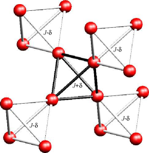
Figure 1: The pyrochlore structure. The tetrahedra alternate between two orientations (black/white). In the presence of a breathing mode the coupling constants associated with each exchange path will differ depending on which tetrahedron orientation they belong to.

In the following, we present analytic calculations of magnon dispersions for the $\Gamma_{5,6}$ ground state doublet in the presence of an AIAO magnetic state. A bosonic Hamiltonian describing magnons is obtained from the exchange Hamiltonian using the Holstein-Primakoff transformation.T. Holstein and H. Primakoff (1940); Benton (2016) The quadratic bosonic Hamiltonian is exactly diagonalizable for all $\vec{k}$, i.e. the dispersion and the Bogoliubov transformation are presented in analytic form. We find that the breathing mode lifts the degeneracy which otherwise occurs in the upper band along the path between the $X$-point and the $W$-point in $\vec{k}$-space.Lastly, we compute the dynamical structure factor for inelastic neutron scattering.

II Spin Hamiltonian

Considering short-range interactions only, the Hamiltonian for the rare-earth spins has three contributions, the crystal electric field ${\mathcal{H}}_{\rm CEF}$, the nearest-neighbour exchange interaction ${\mathcal{H}}_{\rm ex}$, and the Zeeman term ${\mathcal{H}}_{\rm Z}$,

$${\mathcal{H}}={\mathcal{H}}_{\rm CEF}+{\mathcal{H}}_{\rm ex}+{\mathcal{H}}_{\rm Z}.$$ (1)

For the rare-earth site symmetry $D_{3d}$, there are six independent terms in ${\mathcal{H}}_{\rm CEF}$ which are expressed as Stevens operators.K. W. H. Stevens (1951) The six CEF parameters have been determined (via inelastic neutron scattering experiments) for many compounds in the pyrochlore family.

The energy scale of ${\mathcal{H}}_{\rm CEF}$ is higher than the other terms in ${\mathcal{H}}$, so to lowest order in perturbation theory, we consider the restriction of ${\mathcal{H}}$ to the degenerate ground state of ${\mathcal{H}}_{\rm CEF}$. The result has different forms depending on the symmetry of the CEF of ground state.S. H. Curnoe (2018)For the $\Gamma_{5,6}$ CEF ground state the restricted exchange Hamiltonian takes the general formHuang et al. (2014)

$${\mathcal{H}}^{\Gamma_{5,6}}_{\rm ex} = \sum_{\langle ij\rangle}[J_{z}S_{iz}S_{jz}+J_{y}S_{iy}S_{jy}+J_{x}S_{ix}S_{jx}$$ (2)

$$+J_{zx}(S_{iz}S_{jx}+S_{ix}S_{jz})]$$

where $J_{z}$,$J_{y}$, $J_{x}$ and $J_{zx}$ are exchange constants; the sum is over pairs of nearest-neighbour spins and the subscripts $x,y,z$ refer to local coordinates where the local $z$ axis points along the 3-fold axis of the CEF (see Appendix A). The pseudospin operator $\vec{S}$ acts within the space of the ground state doublet, and is represented by the $2\times 2$ Pauli matrices, $\vec{S}=\frac{1}{2}\vec{\sigma}$. The last term in Eq. 2 can be eliminated by a rotation by an angle $\theta=\frac{1}{2}\tan^{-1}\left(\frac{J_{zx}}{J_{x}-J_{y}}\right)$ about the local $y$-axis, yieldingHuang et al. (2014)

$${\mathcal{H}}_{\rm ex}^{\Gamma_{5,6}}=\sum_{\langle ij\rangle}\left[\tilde{J}_{z}\tilde{S}_{iz}\tilde{S}_{jz}+\tilde{J}_{y}\tilde{S}_{iy}\tilde{S}_{jy}+\tilde{J}_{x}\tilde{S}_{ix}\tilde{S}_{jx}\right]$$ (3)

where $\tilde{S}_{x}$ and $\tilde{S}_{z}$ are rotated operators and $\tilde{J}_{x}$ and $\tilde{J}_{z}$ are renormalized exchange constants resulting from the rotation, which are related to the original constants by $J_{x}=\tilde{J}_{x}\cos^{2}\theta+\tilde{J}_{z}\sin^{2}\theta$ and $J_{z}=\tilde{J}_{x}\sin^{2}\theta+\tilde{J}_{z}\cos^{2}\theta$. Huang et al. (2014); Benton (2016) We also take $\tilde{J}_{y}\equiv J_{y}$ and $\tilde{S}_{y}\equiv S_{y}$. For Nd₂Zr₂O₇, the value of $\theta=0.98$ rad was recently reported, and the exchange constants are $\tilde{J}_{x}=0.091$ meV, $\tilde{J}_{y}=0.014$ meV, and $\tilde{J}_{z}=-0.046$ meV.J. Xu, Owen Benton, V. K. Anand, A. T. M. N. Islam, T. Guidi, G. Ehlers, E. Feng, Y. Su, A. Sakai, P. Gegenwart, and B. Lake (2019)

The pseudospin operators $S_{i\alpha}$ correspond to different dipolar and octupolar physical operators that act on the space of the ground state doublet, in particular $\hat{J}_{z}=jS_{z}+tS_{x}$, where $j$ and $t$ are material dependent parameters that can be computed given an explicit form of the CEF doublet. For example, the CEF ground state for Nd₂Zr₂O₇ isE. Lhotel, S. Petit, S. Guitteny, O. Florea, M. Ciomaga Hatnean, C. Colin, E. Ressouche, M. R. Lees, and G. Balakrishnan (2015)

$$\ket{\pm}=-.878\ket{\mp 9/2}\mp.05\ket{\mp 3/2}+.476\ket{\pm 3/2}\pm.009\ket{\pm 9/2}$$ (4)

from which we compute $j=\langle+|\hat{J}_{z}|+\rangle=-3.13$, and $t=\langle+|\hat{J}_{z}|-\rangle=0.000282$.

For the breathing pyrochlores, we consider the Hamiltonian (3) with the exchange constants replaced by $\tilde{J}_{\alpha}\pm\delta_{\alpha}$ for $\alpha=x,y,z$, where the $\pm$ signs are used at alternating tetrahedra, so that the breathing factors are each of the form $1+2\delta_{\alpha}/\tilde{J}_{\alpha}$. In this work we will make the simplifying assumption that all three $\delta$’s are equal, so the Hamiltonian can be expressed as

$${\mathcal{H}}^{\Gamma_{5,6}}_{\rm Breath}={\mathcal{H}}_{\rm ex}^{\Gamma_{5,6}}+\Delta\mathcal{H},$$ (5)

where

$$\Delta\mathcal{H}=\delta\left[\sum_{\langle ij\rangle\in B}\tilde{\bf S}_{i}\cdot\tilde{\bf S}_{j}-\sum_{\langle ij\rangle\in A}\tilde{\bf S}_{i}\cdot\tilde{\bf S}_{j}\right]$$ (6)

The general case for where the three $\delta$’s are different can be analyzed following the same procedure presented in this work.

III Magnons

To study the low energy excitations of the system we use the Holstein-Primakoff (HP) transformationT. Holstein and H. Primakoff (1940)

$$\tilde{S}_{i+}=\left(\sqrt{2S-a_{i}^{\dagger}a_{i}}\right)a_{i},\tilde{S}_{iz}=S-a_{i}^{\dagger}a_{i}$$ (7)

where $S=1/2$ is the spin quantum number and $a_{i}$ and $a_{i}^{\dagger}$ are bosonic annihilation and creation operators, respectively. The operator defined in Eq. 7 is cumbersome to deal with due to the square root; hence, we rely on the linear spin wave approximation (LSWA) where $\tilde{S}_{i+}\approx\sqrt{2S}a_{i}$. In magnetic states, the direction for the pseudospin operators is generally not the same as the direction of the physical momentum. For example, in Nd₂Zr₂O₇ the pseudospin operators aligned at an angle $\theta$ with respect to the local $z$-direction defined in Appendix A, which is the direction of the physical momenta in the AIAO ground state.Benton (2016); E. Lhotel, S. Petit, M. Ciomaga Hatnean, J. Ollivier, H. Mutka, E. Ressouche, M. R. Lees, and G. Balakrishnan (2018); J. Xu, Owen Benton, V. K. Anand, A. T. M. N. Islam, T. Guidi, G. Ehlers, E. Feng, Y. Su, A. Sakai, P. Gegenwart, and B. Lake (2019)

Applying the LSWA to the Hamiltonian in Eq. (3), we obtain a bosonic Hamiltonian

$${\mathcal{H}}_{\rm ex}^{\Gamma_{5,6}}\approx\frac{3N}{4}\tilde{J}_{z}+{\mathcal{H}}_{2}$$ (8)

where $N$ is the total number of magnetic ions and ${\mathcal{H}}_{2}$ is quadratic in $a$ and $a^{\dagger}$. Using the Fourier transform of the bosonic operators, the quadratic bosonic Hamiltonian is

$${\mathcal{H}}_{2}=\sum_{\vec{k}}L^{\dagger}_{\vec{k}}M(\vec{k})L_{\vec{k}}$$ (9)

where

$$L_{\vec{k}}=\left(\begin{array}[]{ c c c c l r }a_{1}(\vec{k}),..,a_{4}(\vec{k}),a^{\dagger}_{1}(-\vec{k}),..,a^{\dagger}_{4}(-\vec{k})\end{array}\right)^{T},$$ (10)

and

$$M(\vec{k})=\left(\begin{array}[]{ c c c c c c l r }\mathcal{J}^{+}R-3\tilde{J}_{z}{\mathbf{1}}&\mathcal{J}^{-}R\\ \mathcal{J}^{-}R&\mathcal{J}^{+}R-3\tilde{J}_{z}{\mathbf{1}}\\ \end{array}\right).$$ (11)

Here ${\mathbf{1}}$ is the $4\times 4$ identity matrix, $\mathcal{J}^{\pm}=\frac{\tilde{J}_{x}\pm\tilde{J}_{y}}{2}$, and $R(\vec{k})$ is a $4\times 4$ matrix with components

$$R_{ij}(\vec{k})=\cos\left[\vec{k}\cdot(\vec{r}_{i}-\vec{r}_{j})\right]-\delta_{ij},$$ (12)

where $\vec{r}_{i}$ is the position within a primitive unit cell of the $i$th ($i=1,2,3,4$) magnetic ion.

The next step is to diagonalize ${\mathcal{H}}_{2}$ by finding a Bogoliubov transformation of the form $L_{\vec{k}}=Z{\mathcal{L}}_{\vec{k}}$, where $Z$ is an $8\times 8$ matrix containing the Bogoliubov coefficients and

$${\mathcal{L}}_{\vec{k}}=\left(\begin{array}[]{ c c c c l r }b_{1}(\vec{k}),..,b_{4}(\vec{k}),b^{\dagger}_{1}(-\vec{k}),..,b^{\dagger}_{4}(-\vec{k})\\ \end{array}\right)^{T}$$ (13)

defines a new set of new bosonic operators. The construction of the Bogoliubov matrix $Z$ is discussed in Appendix B. The diagonalized version of Eq. 9 is

$${\mathcal{H}}_{2}=\sum_{\vec{k}}\sum_{\nu}\varepsilon_{\nu}(\vec{k})\left[b_{\nu}^{\dagger}(\vec{k})b_{\nu}(\vec{k})+b_{\nu}^{\dagger}(-\vec{k})b_{\nu}(-\vec{k})\right]$$ (14)

up to some additive constant.

For the breathing lattice, we find that to $M(k)$ (Eq. 11) we add the matrix

$$W(\vec{k})=i\delta\left(\begin{array}[]{cc}\eta(\vec{k})&0\\ 0&\eta(\vec{k})\end{array}\right)$$ (15)

where $\eta(\vec{k})$ is a $4\times 4$ matrix with components $\eta_{ij}(\vec{k})=\sin\left[\vec{k}\cdot(\vec{r}_{i}-\vec{r}_{j})\right]$.

In the next section, we apply the procedure presented in the Appendices to analytically determine the Bogoliubov transformation matrix and magnon dispersions for an AIAO magnetic state with a $\Gamma_{5,6}$ CEF ground state doublet. We also examine the effect of a breathing mode on the dispersion.

IV Results and Discussion

IV.1 Energy Dispersion

IV.1.1 Undistorted Lattice

We first consider magnons described by the bosonic Hamiltonian (9) in the absence of any breathing mode. According to the results derived in Appendix C, the magnon dispersions are

$$\varepsilon_{\nu}(\vec{k})=\sqrt{(3\tilde{J}_{z}-\tilde{J}_{x}r_{\nu})(3\tilde{J}_{z}-\tilde{J}_{y}r_{\nu})}$$ (16)

where $r_{1,2}=-1$ and $r_{3,4}=1\pm\gamma(\vec{k})$, with

$$\gamma^{2}(\vec{k}) = 1+\cos(ak_{x}/2)\cos(ak_{y}/2)+\cos(ak_{y}/2)\cos(ak_{z}/2)$$ (17)

$$+\cos(ak_{z}/2)\cos(ak_{x}/2),$$

in agreement with numerical results previously reported.Benton (2016); H. Yan, O. Benton, L. Jaubert, and N. Shannon (2017) Two bands are doubly degenerate and non-dispersive,

$$\varepsilon_{1,2}=\sqrt{(3\tilde{J}_{z}+\tilde{J}_{x})(3\tilde{J}_{z}+\tilde{J}_{y})}.$$ (18)

IV.1.2 Breathing lattice

Here we present the solution to the magnonic Hamilton on a breathing lattice,

$${\mathcal{H}}_{\rm breath}=\sum_{\vec{k}}L^{\dagger}_{\vec{k}}(M(\vec{k})+W(\vec{k}))L_{\vec{k}}$$ (19)

where $L(\vec{k})$, $M(\vec{k})$ and $W(\vec{k})$ are given by Eqs. 10, 11 and 15. Analytic expressions for the band dispersions are derived in Appendix E. The degenerate non-dispersive bands $\varepsilon_{1,2}$ remain unchanged in the presence of a breathing mode, at least within the LSWA and other assumptions used here. However, the presence of a breathing mode is reflected in the dispersive bands, which are modified to

$$\varepsilon^{2}_{3,4}(\vec{k})=b(\vec{k})\pm\sqrt{b^{2}(\vec{k})-c(\vec{k})},$$ (20)

where

$$b(\vec{k})=\sigma(\tilde{J}_{x},\tilde{J}_{y},\tilde{J}_{z},\vec{k})-6\tilde{J}_{z}(\tilde{J}_{x}+\tilde{J}_{y})+2\tilde{J}_{x}\tilde{J}_{y}+18\tilde{J}_{z}^{2},$$ (21)

$$c(\vec{k})=\sigma(\tilde{J}_{x},\tilde{J}_{x},\tilde{J}_{z},\vec{k})\sigma(\tilde{J}_{y},\tilde{J}_{y},\tilde{J}_{z},\vec{k}),$$ (22)

and

$$\sigma(J_{x},J_{y},J_{z},\vec{k}) = \left(\gamma^{2}(\vec{k})-1\right)\left(J_{x}J_{y}-\delta^{2}\right)$$ (23)

$$+3\left(\delta^{2}+(J_{x}+J_{y})J_{z}-3J_{z}^{2}\right).$$

As an example, we compute the magnon spectrum using the exchange constants of ${\rm Nd_{2}Zr_{2}O_{7}}$ which were reported in Ref. J. Xu, Owen Benton, V. K. Anand, A. T. M. N. Islam, T. Guidi, G. Ehlers, E. Feng, Y. Su, A. Sakai, P. Gegenwart, and B. Lake, 2019. In Fig. 2 we plot the magnon energies using $\delta=0$ (no distortion) and $\delta=0.004$ meV. We find that a breathing mode distortion is reflected on the $k$-space path between the $X$ and $W$ points, where the degeneracy of the top band is lifted, resulting in a gap between the two upper bands, similar to the findings in Ref. Essafi et al., 2017b. The gap $\Delta$ between the upper bands along the path $X\to W$ is linear in $\delta$,

$$\Delta\approx\frac{2(\tilde{J}_{x}+\tilde{J}_{y}-6\tilde{J}_{z})}{\sqrt{(\tilde{J}_{x}-3\tilde{J}_{z})(\tilde{J}_{y}-3\tilde{J}_{z})}}\delta.$$ (24)

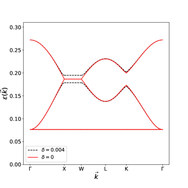
Figure 2: Magnon dispersions computed using the exchange constants of Nd₂Zr₂O₇ (discussed in the text) with $\delta=0$ (red solid) and $\delta=0.004$ meV (black dashed).

IV.2 The dynamical structure factor

An important quantity that is experimentally accessible through inelastic neutron scattering is the dynamical structure factor,H. Yan, O. Benton, L. Jaubert, and N. Shannon (2017)

$$\mathcal{S}(\vec{q},\omega) = \int dte^{-i\omega t}\sum_{\alpha\beta}\left(\delta_{\alpha\beta}-\frac{q_{\alpha}q_{\beta}}{q^{2}}\right)$$ (25)

$$\times\sum_{i,j=1}^{4}\langle\hat{J}_{i}^{\alpha}(-\vec{q},0)\hat{J}_{j}^{\beta}(\vec{q},t)\rangle$$

where $i=1,2,3,4$ is the site number within the primitive unit cell, and $\alpha=x,y,z$ refer to global axes. Eqn. 25 can be expressed in terms of the momenta for local axes $\hat{J}_{i\alpha}$ using the definitions in Appendix A, however in the restriction to the dipolar-octupolar ($\Gamma_{5,6}$) CEF doublet, the only non-vanishing component of the physical angular momentum is $\hat{J}_{iz}$. Finally, these are related to the pseudo-spin operators introduced in Eqs. 2 and 3. In the LSWA, only the transverse components components (perpendicular to $\tilde{S}_{z}$) contribute to the spin-spin correlation function. Our analytic form of the Bogoluibov transformation (contructed in Appendices D and E) is used to express the spin-spin correlation function in terms of the normal modes (magnons). The dynamical structure factor is shown in Fig. 3 for different values of the lattice distortion.

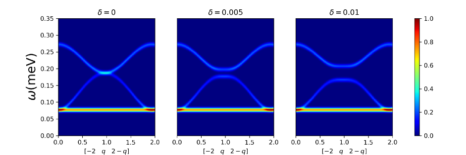
(a)

Figure 3: The dynamical structure factor along the direction computed using $\tilde{J}_{x}=0.091$ meV, $\tilde{J}_{y}=0.014$ meV, and $\tilde{J}_{z}=-0.046$ meV, $\theta=0.98$ rad, and lattice distortion $\delta=0$ meV (left), $\delta=0.005$ meV (middle), and $\delta=0.010$ meV (right). We set the temperature to 0 K and a Gaussian standard deviation of 0.004.

Fig. 3 shows the intensity map of the dynamical structure factor along the line $[-2\,\,q\,\,2-q]$. The most pronounced changes to the magnon dispersions occur in the vicinity of $[-2\,\,1\,\,1]$, which is equivalent to the $X$-point of the first Brillioun zone. Here in the presence of a breathing mode the degeneracy is lifted and there is a distinct flattening of the bands.

V Conclusions

In this work we presented the exact analytic diagonalization of the magnon Hamiltonian for magnetic pyrochlores in the linear spin wave approximation, applied to the special case where the magnetic ions have a $\Gamma_{5,6}$ CEF ground state doublet with an ordered AIAO magnetic ground state.Benton (2016); H. Yan, O. Benton, L. Jaubert, and N. Shannon (2017) As an illustration, we applied our findings to Nd₂Zr₂O₇ for which the exchange constants and the CEF states are known.Benton (2016); E. Lhotel, S. Petit, M. Ciomaga Hatnean, J. Ollivier, H. Mutka, E. Ressouche, M. R. Lees, and G. Balakrishnan (2018); J. Xu, Owen Benton, V. K. Anand, A. T. M. N. Islam, T. Guidi, G. Ehlers, E. Feng, Y. Su, A. Sakai, P. Gegenwart, and B. Lake (2019) We also considered the breathing pyrochlore lattice and found the analytic form of the energy dispersion for all $\vec{k}$. In the special case we considered, the signature of a lattice distortion is the degeneracy-lifting of the upper magnon band between the $X$ and $W$ points in $k$-space.

Appendix A The local reference frame

The primitive unit cell of the RE system is a single tetrahedron with the four rare earth ions at the positions $(5/8,5/8,5/8)$, $(3/8,3/8,5/8)$, $(3/8,5/8,3/8)$ and $(5/8,3/8,3/8)$ for site numbers 1, 2, 3, and 4 respectively. We define a local coordinate system such that the local $z$-axes are the the $C_{3}$ axes for each site:

$$\hat{x}_{1}=(1,1,-2)/\sqrt{6} \hat{x}_{2}=(-1,-1,-2)/\sqrt{6}$$

$$\hat{y}_{1}=(-1,1,0)/\sqrt{2} \hat{y}_{2}=(1,-1,0)/\sqrt{2}$$

$$\hat{z}_{1}=(1,1,1)/\sqrt{3} \hat{z}_{2}=(-1,-1,1)/\sqrt{3}$$

$$\hat{x}_{3}=(-1,1,2)/\sqrt{6} \hat{x}_{4}=(1,-1,2)/\sqrt{6}$$

$$\hat{y}_{3}=(1,1,0)/\sqrt{2} \hat{y}_{4}=(-1,-1,0)/\sqrt{2}$$

$$\hat{z}_{3}=(-1,1,-1)/\sqrt{3} \hat{z}_{4}=(1,-1,-1)/\sqrt{3}$$

Appendix B The Bogoliubov transformation matrix

The main task here is to find the Bogoliubov transformation matrix $Z$ which satisfies the following conditions simultaneously:

$$Z^{-1}{\mathcal{G}}MZ = \left(\begin{array}[]{cc}{\mathcal{E}}&0\\ 0&-{\mathcal{E}}\\ \end{array}\right)$$ (28)

$$Z{\mathcal{G}}Z^{\dagger} = {\mathcal{G}}=\left(\begin{array}[]{ c c c c c c l r }{\mathbf{1}}&\mathbf{0}\\ \mathbf{0}&-{\mathbf{1}}\\ \end{array}\right),$$ (31)

$$Z^{\dagger}MZ = \left(\begin{array}[]{cc}{\mathcal{E}}&0\\ 0&{\mathcal{E}}\\ \end{array}\right)$$ (34)

where $M$ is the $8\times 8$ matrix given by Eq. 11. We assume that ${\mathcal{G}}M$ has $q$ distinct eigenvalues (where $q\leq 8$), each with degeneracy $d_{i}$.Del Maestro and Gingras (2004) We begin by finding the normalized eigenvectors of ${\mathcal{G}}M$ and arranging their components in columns, such that the eigenvectors belonging to the same eigenvalue are next to each other. We call this matrix $\tilde{Z}$. Next, we assume that there is a block-diagonal matrix $P$, such that $Z=\tilde{Z}P$, where the sizes of the blocks of $P$ are $d_{i}\times d_{i}$. Considering Eq. 31 and that ${\mathcal{G}}^{-1}={\mathcal{G}}$, we haveDel Maestro and Gingras (2004)

$$P{\mathcal{G}}P^{\dagger}=(\tilde{Z}^{\dagger}{\mathcal{G}}\tilde{Z})^{-1}.$$ (35)

By construction, the matrix $W=(\tilde{Z}^{\dagger}{\mathcal{G}}\tilde{Z})^{-1}$ is Hermitian and block-diagonal, with $q$ blocks with dimensions $d_{i}\times d_{i}$. For each block we write

$$\pm P_{i}P_{i}^{\dagger}=W_{i}$$ (36)

where the sign is positive for blocks in the upper half of $P$ and negative otherwise. Since each block $W_{i}$ is Hermitian, each $W_{i}$ can be diagonalized by a unitary matrix $X_{i}$,

$$W_{i}=X_{i}D_{i}X_{i}^{-1}$$ (37)

where $D_{i}$ is a diagonal matrix containing the eigenvalues of $W_{i}$. Consequently, the solution of $P_{i}$ isDel Maestro and Gingras (2004)

$$P_{i}=X_{i}\sqrt{\pm D_{i}}X_{i}^{-1}.$$ (38)

Thus, we can construct the Bogoliubov transformation matrix $Z=\tilde{Z}P$.

Appendix C Eigenvalues and eigenvectors of $R$ and $\eta$

In this appendix we present analytic forms for the eigenvalues and eigenvectors of the matrix $R$ (see Eq. 11). The results will be used in Appendix D to find the analytic form of the magnon dispersions and to construct the Bogliubov transformation. To shorten the notation we use $\{\cos(ak/4),\sin(ak/4)\}=\{c(k),s(k)\}$. The eigenvalues of $R$ are

$$r_{1}=r_{2}=-1,\;\;\;r_{3,4}\equiv r_{\pm}=1\pm\gamma$$ (39)

where $\gamma^{2}=1+c(2k_{x})c(2k_{y})+c(2k_{y})c(2k_{z})+c(2k_{z})c(2k_{x})$ (as in Eq. 17). The eigenvectors of $R$ corresponding to $r_{1,2}=-1$ are

$$\Bigg{\{}\left[\begin{array}[]{cccc}s\left(k_{x}-k_{z}\right)\\ s\left(k_{y}+k_{z}\right)\\ 0\\ -s\left(k_{x}+k_{y}\right)\\ \end{array}\right],\left[\begin{array}[]{cccc}s\left(k_{y}-k_{z}\right)\\ s\left(k_{x}+k_{z}\right)\\ -s\left(k_{x}+k_{y}\right)\\ 0\\ \end{array}\right]\Bigg{\}}.$$ (40)

Note that these are not orthogonal as they correspond to the same eigenvalue. However, orthogonal eigenvectors can be easily found as simple linear combinations. We call the orthonormalized eigenvectors $\vec{v}_{1}$ and $\vec{v}_{2}$.

We write the other two eigenvectors (corresponding to $r_{3,4}$) as

$$\vec{u}_{3,4}=\vec{u}_{\pm}=\left[\begin{array}[]{cccc}f_{1}^{\pm},f_{2}^{\pm},f_{3}^{\pm},f_{4}^{\pm}\end{array}\right]^{T}$$ (41)

where

$$f_{n}^{\pm}(\vec{k})=g_{n}(\vec{k})+r_{\pm}c(\vec{k}\cdot\vec{r}_{n})$$ (42)

and $\vec{r}_{n}$ is the position of the $n$th rare-earth ion within the primitive cell. The functions $g_{n}(\vec{k})$ are

$$g_{n}(\vec{k})=\begin{cases}\phi(k_{x},k_{y}-k_{z},k_{y}+k_{z})&\quad n=1\\ -\phi(k_{z},k_{y}-k_{x},\pi/2)&\quad n=2\\ -\phi(-k_{y},k_{z}-k_{x},\pi/2)&\quad n=3\\ -\phi(-k_{x},k_{y}-k_{z},\pi/2)&\quad n=4\\ \end{cases}$$ (43)

where

$$\phi(x,y,z)=c(2x+z)c(y)+c^{2}(z).$$ (44)

The normalized eigenvectors are $\vec{v}_{\pm}=\frac{\vec{u}_{\pm}}{||\vec{u}_{\pm}||}$. One can easily verify that $\vec{v}_{\pm}\cdot\vec{v}_{1,2}=0$ for all $\vec{k}$. The orthonormalized version of this set of eigenvectors is needed for the analytic calculation of the Bogoliubov matrix $Z$, as discussed in Appendices D and E.

$R$ and $\eta$ share the eigenvectors $\vec{v}_{1,2}$ (Eq. 40) and the corresponding eigenvalues for $\eta$ are $0$ (doubly degenerate), i.e. $\eta\vec{v}_{1,2}=0$. To find the other two eigenvectors of $\eta$ we consider the following. One can easily verify the relations between $\eta$ and $R$:

$$\{R-\bm{1},\eta\}=0,\quad\eta^{2}=R^{2}-2R-3.$$ (45)

Also, the action of $\eta$ on $\vec{v}_{\pm}$ is

$$\eta\vec{v}_{\pm}=\sqrt{\gamma^{2}-4}\vec{v}_{\mp}.$$ (46)

Consequently, the other two eigenvectors of $\eta$ are

$$\vec{z}_{3,4}=\vec{v}_{+}\pm\vec{v}_{-}$$ (47)

with eigenvalues $\pm\sqrt{\gamma^{2}-4}$, which are generally complex away from the $\Gamma$ point.

Appendix D Analytic diagonalization of the magnonic Hamiltonian for an undistorted lattice

We can write the matrix ${\mathcal{G}}M$ in the form

$${\mathcal{G}}M(k)=\left(\begin{array}[]{ c c c c c c l r }\mathcal{A}&\mathcal{B}\\ -\mathcal{B}&-\mathcal{A}\\ \end{array}\right)$$ (48)

where $\mathcal{A}={\cal J}^{+}R-3\tilde{J}_{z}{\bf 1}$, $\mathcal{B}={\cal J}^{-}R$, and $R$ and ${\cal J}^{\pm}$ are defined after Eq. 11. The eigenvalue equation for a matrix of this form (with $\mathcal{A}$ and $\mathcal{B}$ commuting matrices) reduces to the secular determinantI. Kovacs, D. S. Silver, and S. G. Williams (1999)

$$|(\mathcal{A}^{2}-\mathcal{B}^{2})-\varepsilon^{2}\mathbf{1}|=(\tilde{J}_{x}\tilde{J}_{y})^{4}|R^{2}-aR+b\mathbf{1}|=0,$$ (49)

where $a=\frac{3\tilde{J}_{z}(\tilde{J}_{x}+\tilde{J}_{y})}{\tilde{J}_{x}\tilde{J}_{y}}$ and $b=\frac{(9\tilde{J}_{z}^{2}-\varepsilon^{2})}{\tilde{J}_{x}\tilde{J}_{y}}$. This reduces to $b=r(a-r)$, where $r$ are the eigenvalues of $R$. Solving for $\varepsilon$, we obtain the general form of the magnon dispersions given in Eq. 16.

To find the full Bogoliubov transformation, we first apply the unitary transformation

$${\mathcal{U}}=\frac{1}{\sqrt{2}}\left(\begin{array}[]{ c c c c c c l r }\mathbf{1}&\mathbf{1}\\ -\mathbf{1}&\mathbf{1}\\ \end{array}\right)$$ (50)

to ${\mathcal{G}}M(k)$. We obtain

$${\mathcal{U}}{\mathcal{G}}M{\mathcal{U}}^{\dagger}=\left(\begin{array}[]{cc}\mathbf{0}&-(\mathcal{A}-\mathcal{B})\\ -(\mathcal{A}+\mathcal{B})&\mathbf{0}\\ \end{array}\right).$$ (51)

Now, one can easily verify that the normalized eigenvectors of the $8\times 8$ matrix ${\mathcal{U}}{\mathcal{G}}M{\mathcal{U}}^{\dagger}$ are

$$\vec{\tilde{X}}^{\pm}_{i}=\left[1+\left(\frac{-\tilde{J}_{x}r_{i}+3\tilde{J}_{z}}{\varepsilon_{i}}\right)^{2}\right]^{-\frac{1}{2}}\Bigg{(}\begin{array}[]{ c c c c c c l r }\vec{v}_{i}\\ \pm\frac{-\tilde{J}_{x}r_{i}+3\tilde{J}_{z}}{\varepsilon_{i}}\vec{v}_{i}\\ \end{array}\Bigg{)},$$ (52)

where $\vec{v}_{i}$ are the orthonormal eigenvectors of the matrix $R$ (see Eqns. 40 and 41). Consequently, using the unitary matrix ${\mathcal{U}}$, we find the normalized eigenvectors of ${\mathcal{G}}M$ to be

$$\vec{X}_{i}^{\pm}={\mathcal{U}}^{\dagger}\vec{\tilde{X}}^{\pm}_{i}=\left(\begin{array}[]{ c c c c c c l r }\vec{w}_{i}^{\mp}\\ \vec{w}_{i}^{\pm}\\ \end{array}\right)$$ (53)

where

$$\vec{w}_{i}^{\pm}=\frac{1\pm\frac{-\tilde{J}_{x}r_{i}+3\tilde{J}_{z}}{\varepsilon_{i}}}{\sqrt{2+2\left(\frac{-\tilde{J}_{x}r_{i}+3\tilde{J}_{z}}{\varepsilon_{i}}\right)^{2}}}\vec{v}_{i}.$$

Next, we use the eigenvectors of ${\mathcal{G}}M$ to construct the matrix $\tilde{Z}$ (see Appendix B). Lastly, to find the Bogoliubov matrix $Z$, we follow the procedure described in Appendix B by which we find the matrix $P$ and calculate $Z=\tilde{Z}P$. The matrix ${\mathcal{G}}M$ has 6 unique eigenvalues of which two are doubly degenerate (corresponding to the flat bands). Thus, the matrix $P$ has six blocks where two of them are $2\times 2$ diagonal blocks and the rest are $1\times 1$. Thus, $P$ is a diagonal matrix of the form $P={\rm diag}[p_{1},..,p_{4},p_{1},..p_{4}]$, where

$$p_{i}=\frac{1}{2}\sqrt[4]{\frac{3\tilde{J}_{z}-\tilde{J}_{y}r_{i}}{3\tilde{J}_{z}-\tilde{J}_{x}r_{i}}}\sqrt{2+2\left(\frac{-\tilde{J}_{x}r_{i}+3\tilde{J}_{z}}{\varepsilon_{i}}\right)^{2}}.$$ (54)

Defining $\vec{z}_{i}^{\pm}=p_{i}\vec{w}_{i}^{\pm}$, and $Q_{\pm}=\left(\begin{array}[]{cccc}\vec{z}_{1}^{\pm}&\vec{z}_{2}^{\pm}&\vec{z}_{3}^{\pm}&\vec{z}_{4}^{\pm}\end{array}\right)$, we write the Bogoliubov matrix in block form as

$$Z=\left(\begin{array}[]{cc}Q_{-}&Q_{+}\\ Q_{+}&Q_{-}\\ \end{array}\right)$$ (55)

which satisfies Eqs. (28-34).

Appendix E Analytic Diagonalization for breathing lattice

Following the same procedure in the previous appendix, we find that

$${\mathcal{U}}{\mathcal{G}}M{\mathcal{U}}^{\dagger}=\left(\begin{array}[]{cc}\mathbf{0}&-(\mathcal{A}+i\delta\eta-\mathcal{B})\\ -(\mathcal{A}+i\delta\eta+\mathcal{B})&\mathbf{0}\\ \end{array}\right).$$ (56)

The eigenvalue equation $|{\mathcal{U}}{\mathcal{G}}M{\mathcal{U}}^{\dagger}-\varepsilon|=0$ reduces to the following $4\times 4$ secular determinantI. Kovacs, D. S. Silver, and S. G. Williams (1999)

$$|({\mathcal{A}}+i\delta\eta(k))^{2}-{\mathcal{B}}^{2}\pm i\delta\mathcal{J}^{-}[R,\eta]-\varepsilon^{2}(k)|=0,$$ (57)

where the $\pm$ follows from the properties of Schur determinants.I. Kovacs, D. S. Silver, and S. G. Williams (1999) Without loss of generality, we will consider the $+$ sign and solve the eigenvalue equation $|\Lambda-\varepsilon^{2}(k)|=0$, where $\Lambda=({\mathcal{A}}+i\delta\eta(k))^{2}-{\mathcal{B}}^{2}+i\delta\mathcal{J}^{-}[R,\eta]$. The general form of the eigenvectors is a linear combination of the orthonormalized eigenvectors of $R$:

$$\vec{y}=c_{1}\vec{v}_{1}+c_{2}\vec{v}_{2}+c_{3}\vec{v}_{3}+c_{4}\vec{v}_{4}.$$ (58)

Defining $\vec{c}=(c_{1},c_{2},c_{3},c_{4})^{T}$, we map the eigenvalue equation to one using the eigenvectors of $R$ as the basis vectors:

$$\left(\begin{array}[]{cc}\Omega_{1}&\bm{0}\\ \bm{0}&\Omega_{2}\\ \end{array}\right)\vec{c}=\varepsilon^{2}\vec{c}$$ (59)

where $\Omega_{1}$ and $\Omega_{2}$ are $2\times 2$ matrices,

$$\Omega_{1} = \left[(\mathcal{J}^{+}+3\tilde{J}_{z})^{2}-(\mathcal{J}^{-})^{2}\right]\bm{1},$$ (60)

$$\Omega_{2} = \left(\begin{array}[]{cc}a_{-}^{2}-\delta^{2}t^{2}-b_{-}^{2}&i\delta t\left[a_{+}+a_{-}-2\gamma\mathcal{J}^{-}\right]\\ i\delta t\left[a_{+}+a_{-}+2\gamma\mathcal{J}^{-}\right]&a_{+}^{2}-\delta^{2}t^{2}-b_{+}^{2}\end{array}\right)$$ (63)

and $a_{\pm}=\mathcal{J}^{+}r_{\pm}-3\tilde{J}_{z}$, $b_{\pm}=\mathcal{J}^{-}r_{\pm}$, and $t=\sqrt{\gamma^{2}-4}$. The eigenvalues of $\Omega_{1}$ are $(\mathcal{J}^{+}+3\tilde{J}_{z})^{2}-(\mathcal{J}^{-})^{2}$ (doubly degenerate) producing the flat bands in Eq. 18, and the eigenvalues of $\Omega_{2}$ are the dispersive bands energies (squared) given by Eqs. 20 - 23.

Next, we calculate the Bogoliubov matrix $Z$. Let $X=\left(\begin{array}[]{cc}x_{11}&x_{12}\\ x_{21}&x_{22}\\ \end{array}\right)$ be a $2\times 2$ matrix that diagonalizes $\Omega_{2}$; that is, $\Omega_{2}=XDX^{-1}$, where $D$ is a diagonal matrix containing the eigenvalues of $\Omega_{2}$. For a $2\times 2$ matrix $X$ is easily found. Then the matrix that diagonalizes the $4\times 4$ matrix in Eq. 59 is

$$W=\left(\begin{array}[]{cc}\bm{1}&\bm{0}\\ \bm{0}&X\\ \end{array}\right).$$ (65)

Thus, we conclude that the four eigenvectors of $\Lambda$ are

$$\vec{y}_{1}=\vec{v}_{1}, \vec{y}_{2}=\vec{v}_{2},$$ (66)

$$\vec{y}_{3}=x_{11}\vec{v}_{3}+x_{21}\vec{v}_{4}, \quad{\rm and}\quad \vec{y}_{4}=x_{12}\vec{v}_{3}+x_{22}\vec{v}_{4}.$$ (67)

Using this information, we find that the eigenvectors of ${\mathcal{G}}M$ are of the form

$$\vec{X}^{\pm}_{i}=\frac{1}{\sqrt{2}}\left(\begin{array}[]{cc}\pm\varepsilon_{i}^{-1}{\mathcal{C}}&-\mathbf{1}\\ \pm\varepsilon_{i}^{-1}{\mathcal{C}}&\mathbf{1}\\ \end{array}\right)\left(\begin{array}[]{cc}\vec{y}_{i}\\ \vec{y}_{i}\\ \end{array}\right),$$ (68)

where ${\mathcal{C}}=-({\mathcal{A}}+i\delta\eta-{\mathcal{B}})$. Using these vectors, we can determine $\tilde{Z}=\left(\begin{array}[]{ccccccccccccc}\vec{X}^{+}_{1}&\cdots&\vec{X}^{+}_{4}&\vec{X}^{-}_{1}&\cdots&\vec{X}^{-}_{4}\end{array}\right)$, which we then use to find the matrix

$$\tilde{Z}^{\dagger}{\mathcal{G}}\tilde{Z}=\left(\begin{array}[]{cc}F^{(1)}&F^{(2)}\\ F^{(3)}&F^{(4)}\\ \end{array}\right),$$ (69)

where $F^{(1)}_{ij}=-(\varepsilon_{i}^{-1}+\varepsilon_{j}^{-1})\vec{y}_{i}\cdot{\mathcal{C}}\vec{y}_{j}$, $F^{(2)}_{ij}=-(\varepsilon_{i}^{-1}-\varepsilon_{j}^{-1})\vec{y}_{i}\cdot{\mathcal{C}}\vec{y}_{j}=0=F^{(3)}_{ij}$ and $F^{(4)}_{ij}=(\varepsilon_{i}^{-1}+\varepsilon_{j}^{-1})\vec{y}_{i}\cdot{\mathcal{C}}\vec{y}_{j}=-F^{(1)}_{ij}$. Using the relation $W^{-1}=\tilde{Z}^{\dagger}{\mathcal{G}}\tilde{Z}$ together with Eq. 36, we find $P={\rm diag}[p_{1},..,p_{4},p_{1},..p_{4}]$, where

$$p_{i}=\sqrt{-\frac{\varepsilon_{i}}{2\vec{y}_{i}\cdot{\mathcal{C}}\vec{y}_{i}}}.$$ (70)

Finally the Bogoliubov matrix for the breathing lattice is $Z=\tilde{Z}P$.

References

- Harris et al. (1997) M. J. Harris, S. T. Bramwell, D. F. McMorrow, T. Zeiske, and K. W. Godfrey, Phys. Rev. Lett. 79, 2554 (1997).
- Ramirez et al. (1999) A. P. Ramirez, A. Hayashi, R. J. Cava, R. Siddharthan, and B. S. Shastry, Nature 399, 333 (1999).
- Gardner et al. (2001) J. S. Gardner, B. D. Gaulin, A. J. Berlinsky, P. Waldron, S. R. Dunsiger, N. P. Raju, and J. E. Greedan, Phys. Rev. B 64, 224416 (2001).
- Champion et al. (2003) J. D. M. Champion, M. J. Harris, P. C. W. Holdsworth, A. S. Wills, G. Balakrishnan, S. T. Bramwell, E. Čižmár, T. Fennell, J. S. Gardner, J. Lago, D. F. McMorrow, M. Orendáč, A. Orendáčová, D. M. Paul, R. I. Smith, M. T. F. Telling, and A. Wildes, Phys. Rev. B 68, 020401 (2003).
- E. Lhotel, S. Petit, S. Guitteny, O. Florea, M. Ciomaga Hatnean, C. Colin, E. Ressouche, M. R. Lees, and G. Balakrishnan (2015) E. Lhotel, S. Petit, S. Guitteny, O. Florea, M. Ciomaga Hatnean, C. Colin, E. Ressouche, M. R. Lees, and G. Balakrishnan, Phys. Rev. Lett. 115, 197202 (2015).
- J. Xu, Owen Benton, V. K. Anand, A. T. M. N. Islam, T. Guidi, G. Ehlers, E. Feng, Y. Su, A. Sakai, P. Gegenwart, and B. Lake (2019) J. Xu, Owen Benton, V. K. Anand, A. T. M. N. Islam, T. Guidi, G. Ehlers, E. Feng, Y. Su, A. Sakai, P. Gegenwart, and B. Lake, Phys. Rev. B 99, 144420 (2019).
- S. H. Curnoe (2008) S. H. Curnoe, Phys. Rev. B 78, 094418 (2008).
- H. Yan, O. Benton, L. Jaubert, and N. Shannon (2017) H. Yan, O. Benton, L. Jaubert, and N. Shannon, Phys. Rev. B 95, 094422 (2017).
- K. A. Ross, L. Savary, B. D. Gaulin, and L. Balents (2011) K. A. Ross, L. Savary, B. D. Gaulin, and L. Balents, Phys. Rev. X 1, 021002 (2011).
- L. Savary, K. A. Ross, B. D. Gaulin, J. P. C. Ruff, and L. Balents (2012) L. Savary, K. A. Ross, B. D. Gaulin, J. P. C. Ruff, and L. Balents, Phys. Rev. Lett. 109, 167201 (2012).
- Huang et al. (2014) Y.-P. Huang, G. Chen, and M. Hermele, Phys. Rev. Lett. 112, 167203 (2014).
- Onoda and Tanaka (2010) S. Onoda and Y. Tanaka, Phys. Rev. Lett. 105, 047201 (2010).
- A. Bertin, P. Dalmas de Réotier, B. Fåk, C. Marin, A. Yaouanc, A. Forget, D. Sheptyakov, B. Frick, C. Ritter, A. Amato, C. Baines, and P. J. C. King (2015) A. Bertin, P. Dalmas de Réotier, B. Fåk, C. Marin, A. Yaouanc, A. Forget, D. Sheptyakov, B. Frick, C. Ritter, A. Amato, C. Baines, and P. J. C. King, Phys. Rev. B 92, 144423 (2015).
- V. K. Anand, A. K. Bera, J. Xu, T. Herrmannsdörfer, C. Ritter, and B. Lake (2015) V. K. Anand, A. K. Bera, J. Xu, T. Herrmannsdörfer, C. Ritter, and B. Lake, Phys. Rev. B 92, 184418 (2015).
- K. Tomiyasu, K. Matsuhira, K. Iwasa, M. Watahiki, S. Takagi, M. Wakeshima, Y. Hinatsu, M. Yokoyama, K. Ohoyama, and K. Yamada (2012) K. Tomiyasu, K. Matsuhira, K. Iwasa, M. Watahiki, S. Takagi, M. Wakeshima, Y. Hinatsu, M. Yokoyama, K. Ohoyama, and K. Yamada, J. Phys. Soc. Jpn. 81, 034709 (2012).
- S. Petit, E. Lhotel, B. Canals, M. Ciomaga Hatnean, J. Ollivier, H. Mutka, E. Ressouche, A. R. Wildes, M. R. Lees and G. Balakrishnan (2016) S. Petit, E. Lhotel, B. Canals, M. Ciomaga Hatnean, J. Ollivier, H. Mutka, E. Ressouche, A. R. Wildes, M. R. Lees and G. Balakrishnan, Nat. Phys. 12, 746 (2016).
- Benton (2016) O. Benton, Phys. Rev. B 94, 104430 (2016).
- E. Lhotel, S. Petit, M. Ciomaga Hatnean, J. Ollivier, H. Mutka, E. Ressouche, M. R. Lees, and G. Balakrishnan (2018) E. Lhotel, S. Petit, M. Ciomaga Hatnean, J. Ollivier, H. Mutka, E. Ressouche, M. R. Lees, and G. Balakrishnan, Nature Communications 9, 3786 (2018).
- Y. Okamoto, G. J. Nilsen, J. P. Attfield, and Z. Hiroi (2013) Y. Okamoto, G. J. Nilsen, J. P. Attfield, and Z. Hiroi, Phys. Rev. Lett. 110, 097203 (2013).
- K. Kimura, S. Nakatsuji, and T. Kimura (2014) K. Kimura, S. Nakatsuji, and T. Kimura, Phys. Rev. B 90, 060414 (2014).
- T. Haku, K. Kimura, Y. Matsumoto, M. Soda, M. Sera, D. Yu, R. A. Mole, T. Takeuchi, S. Nakatsuji, Y. Kono, T. Sakakibara, L.-J. Chang, and T. Masuda (2016) T. Haku, K. Kimura, Y. Matsumoto, M. Soda, M. Sera, D. Yu, R. A. Mole, T. Takeuchi, S. Nakatsuji, Y. Kono, T. Sakakibara, L.-J. Chang, and T. Masuda, Phys. Rev. B 93, 220407 (2016).
- Y. Okamoto,, M. Mori, N. Katayama, A. Miyake, M. Tokunaga, A. Matsuo, K. Kindo, and K. Takenaka (2018) Y. Okamoto,, M. Mori, N. Katayama, A. Miyake, M. Tokunaga, A. Matsuo, K. Kindo, and K. Takenaka, J. Phys. Soc. Jpn. 87, 034709 (2018).
- Benton and Shannon (2015) O. Benton and N. Shannon, J. Phys. Soc. Jpn 84, 104710 (2015).
- Li et al. (2016) F.-Y. Li, Y.-D. Li, Y. B. Kim, L. Balents, Y. Yu, and G. Chen, Nature Communications 7, 12691 (2016).
- Savary et al. (2016) L. Savary, X. Wang, H.-Y. Kee, Y. B. Kim, Y. Yu, and G. Chen, Phys. Rev. B 94, 075146 (2016).
- Rau et al. (2016) J. G. Rau, L. S. Wu, A. F. May, L. Poudel, B. Winn, V. O. Garlea, A. Huq, P. Whitfield, A. E. Taylor, M. D. Lumsden, M. J. P. Gingras, and A. D. Christianson, Phys. Rev. Lett. 116, 257204 (2016).
- Essafi et al. (2017a) K. Essafi, L. D. C. Jaubert, and M. Udagawa, J. Phys.: Condensed Matter 29, 315802 (2017a), publisher: IOP Publishing.
- Jian and Nie (2018) S.-K. Jian and W. Nie, Phys. Rev. B 97, 115162 (2018).
- Ezawa (2018) M. Ezawa, Physical Review Letters 120, 026801 (2018), publisher: American Physical Society.
- Aoyama and Kawamura (2019) K. Aoyama and H. Kawamura, Phys. Rev. B 99, 144406 (2019).
- Hirschberger et al. (2019) M. Hirschberger, T. Nakajima, S. Gao, L. Peng, A. Kikkawa, T. Kurumaji, M. Kriener, Y. Yamasaki, H. Sagayama, H. Nakao, K. Ohishi, K. Kakurai, Y. Taguchi, X. Yu, T.-h. Arima, and Y. Tokura, Nat. Commun. 10, 5831 (2019).
- Talanov and Talanov (2020) M. V. Talanov and V. M. Talanov, Cryst. Eng. Comm. 22, 1176 (2020).
- Yan et al. (2020) H. Yan, O. Benton, L. D. C. Jaubert, and N. Shannon, Phys. Rev. Lett. 124, 127203 (2020).
- Wakao et al. (2020) H. Wakao, T. Yoshida, H. Araki, T. Mizoguchi, and Y. Hatsugai, Phys. Rev. B 101, 094107 (2020).
- Gen et al. (2020) M. Gen, Y. Okamoto, M. Mori, K. Takenaka, and Y. Kohama, Phys. Rev. B 101, 054434 (2020).
- Reschke et al. (2020) S. Reschke, F. Meggle, F. Mayr, V. Tsurkan, L. Prodan, H. Nakamura, J. Deisenhofer, C. A. Kuntscher, and I. Kézsmárki, Phys. Rev. B 101, 075118 (2020).
- Shahzad et al. (2020) M. Shahzad, K. Barros, and S. H. Curnoe, Phys. Rev. B 102, 144436 (2020).
- T. Holstein and H. Primakoff (1940) T. Holstein and H. Primakoff, Phys. Rev. 58, 1098 (1940).
- K. W. H. Stevens (1951) K. W. H. Stevens, Proc. Phys. Soc. LXV 3-A (1951).
- S. H. Curnoe (2018) S. H. Curnoe, J. Phys.: Condensed Matter 30, 235803 (2018).
- Essafi et al. (2017b) K. Essafi, L. D. C. Jaubert, and M. Udagawa, J. Phys.: Condensed Matter 29, 315802 (2017b).
- Del Maestro and Gingras (2004) A. G. Del Maestro and M. J. Gingras, J. Phys.: Condensed Matter 16, 3339 (2004).
- I. Kovacs, D. S. Silver, and S. G. Williams (1999) I. Kovacs, D. S. Silver, and S. G. Williams, The American Mathematical Monthly 106, 950 (1999).