Finding Key Structures in MMORPG Graph with Hierarchical Graph Summarization

Abstract

What are the key structures existing in a large real-world MMORPG (Massively Multiplayer Online Role-Playing Game) graph? How can we compactly summarize an MMORPG graph with hierarchical node labels, considering consistent substructures at different levels of hierarchy? Recent MMORPGs generate complex interactions between entities inducing a heterogeneous graph where each entity has hierarchical labels. Succinctly summarizing a heterogeneous MMORPG graph is crucial to better understand its structure; however it is a challenging task since it needs to handle complex interactions and hierarchical labels efficiently. Although there exist few methods to summarize a large-scale graph, they do not deal with heterogeneous graphs with hierarchical node labels.

We propose GSHL, a novel method that summarizes a heterogeneous graph with hierarchical labels. We formulate the encoding cost of hierarchical labels using MDL (Minimum Description Length). GSHL exploits the formulation to identify and segment subgraphs, and discovers compact and consistent structures in the graph. Experiments on a large real-world MMORPG graph with multi-million edges show that GSHL is a useful and scalable tool for summarizing the graph, finding important and interesting structures in the graph, and finding similar users.

1 Introduction

What does a large real-world MMORPG (Massively Multiplayer Online Role-Playing Game) graph look like? What are the key structures existing in a large real-world MMORPG (Massively Multiplayer Online Role-Playing Game) graph? How can we compactly summarize an MMORPG graph with hierarchical node labels, considering consistent substructures at different levels of hierarchy? A large number of interactions between heterogeneous entities appear in MMORPGs, and they are often represented as a heterogeneous graph. For example, a user has several characters, and each character with various equipment visits dungeons. Moreover, each entity has hierarchical labels (i.e., character-dealer-destroyer, and equipment-weapon). Summarizing a heterogeneous graph with hierarchical node labels is a crucial problem to understand its characteristics. A better understanding helps us identify important structures and obtain meaningful insights.

Several approaches have been proposed to summarize graphs using significant structures (vocabularies) commonly found in real-world graphs. VoG [1, 2] is the first approach to summarize a homogeneous graph with vocabulary terms by compressing the graph in terms of Minimum Description Length (MDL) principle. TimeCrunch [3] extended VoG method to summarize dynamic graphs. Both methods, however, fail to summarize a heterogeneous graph with hierarchical labels since they do not excogitate labels of nodes nor the hierarchy of labels.

We propose GSHL (Graph Summarization with Hierarchical Labels), a summarization method for a heterogeneous graph with hierarchical node labels. Based on the MDL principle that good compression leads to good summarization, we precisely define the encoding cost for heterogeneous graphs with hierarchical node labels. GSHL decomposes a heterogeneous graph into subgraphs using a graph decomposition method, and encodes each subgraph as a structure (e.g., star, clique, bipartite core, chain, etc.). Then GSHL further segments each structure by considering hierarchical labels of nodes in the structure, and summarizes the graph using the encoding cost. Thanks to GSHL, we analyze a large real-world MMORPG graph and find its key structures as well as similar users. Our contributions are as follows:

Problem formulation. We formulate the problem of summarizing a heterogeneous graph with hierarchical labels. We use a large real-world graph extracted from Blade & Soul, a popular MMORPG played worldwide. This is the first work in literature that summarizes a large real-world MMORPG graph, to the best of our knowledge.

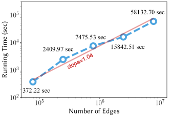
Scalable Method. We propose GSHL, a novel algorithm to summarize a heterogeneous graph with hierarchical node labels. GSHL carefully exploits MDL to encode hierarchical labels, and generates a succinct summary by segmenting subgraphs at different levels of hierarchy. GSHL is near-linear on the number of edges (see Fig. 9).

Experiment. Experiments on the real-world MMORPG graph reveals that GSHL is a useful tool for succinctly summarizing the graph (see Table 4). GSHL discovers interesting patterns (see Fig. 1 and 8), and similar users with similar structures (see Fig. 2).

In the rest of this paper, we describe data, MDL formulation, summary generation, experimental results, related works, and conclusion.

Figure 1: Our hierarchical graph summarization finds more precise and detailed graph structures, compared to non-hierarchical graph summarization. (a) Non-hierarchical graph summarization only finds that an equipment is shared by many characters. It does not recognize the underlying substructures in the characters. (b, c, d) Hierarchical graph summarization finds structures in the lower-level labels of the characters and decomposes the character group into three major substructures with different subgroups.

(a) The most similar account id $3602$

(b) The second most similar account id $9$

Figure 2: The two most similar accounts for account id $0$ share common characters which have similar equipment and visited dungeons. They often share common friends as well.

2 Data Description

Our target data is from Blade & Soul (https://www.bladeandsoul.com/en/), a popular MMORPG played in more than $60$ countries worldwide and earning revenue worth USD $75$ million in $2019$.

2.1 Blade & Soul

Blade & Soul entails multiple characters simultaneously interacting with each other in an open-world environment. Each character carries a variety of equipment acquired throughout its playtime; it enters various dungeons with other characters in order to acquire new equipment or items. Such game design encourages users to repetitively visit dungeons.

A user associated with an account can possess multiple in-game characters with different jobs. These jobs are divided into three types of play-styles: dealer, tanker, and buffer. A dealer mainly afflicts damage to the enemies of its party (a group of multiple characters), while a tanker taunts enemies so the party members can freely afflict damage, and a buffer aids other party members. A party needs to have balanced types of jobs to successfully enter a dungeon and fight with enemies.

Figure 3: Graph structure of Blade & Soul. Accounts have characters which have equipment and dungeons they visited. Accounts are connected to each other via friendship.

(a) Degree distribution of nodes for each level-$1$ label type

(b) Degree distribution of all nodes

(c) Result of SlashBurn

Figure 4: Blade & Soul graph shows a skewed degree distribution.

2.2 Dataset

We collect $3$ months of data from January to March in 2019, and extract the following four relationships.

• account - character: which character(s) each account possesses.

• account - account: friendship between accounts.

• character - dungeon: which dungeons each character visited.

• character - equipment: which equipment each character is equipped with.

We extract $4$ types of entities: account, character, dungeon and equipment. An account represents a user, and a user can have multiple characters. A dungeon entity belongs to a type based on its difficulty where an advanced dungeon is a more difficult version of the corresponding normal dungeon.

2.2.1 Hierarchical Labels

Each label is further divided into sub-labels, and this leads to a hierarchical label structure summarized in Table  1. The four types of entities (account, character, dungeon, and equipment) extracted from the dataset represent level-$1$ of the hierarchy. The account type has no sub-labels. The character type has level-$2$ sub-labels based on play-styles. Each of the level-$2$ label of the character has level-$3$ sub-labels. The dungeon type has $3$ level-$2$ sub-labels. The equipment type has $14$ level-$2$ sub-labels.

Table 1: Hierarchical labels in Blade & Soul graph.

Level-1	Level-2	Level-3	Node Count
Account	$\times$	$\times$	$83,970$
Character	Dealer	Force Master	$19,147$
		Destroyer	23,327
		Summoner	6,266
		Blade Dancer	5,822
		Zen Archer	11,023
	Tanker	Blade Master	11,854
		Kung Fu Master	17,845
		Warden	6,689
	Buffer	Assassin	18,460
		Warlock	15,868
		Soul Fighter	18,249
Dungeon	Normal	$\times$	154
	Advanced	$\times$	12
	Others	$\times$	133
Equipment	Weapon	$\times$	3,219
	Soul Shield	$\times$	3,400
	Ring	$\times$	431
	Bracelet	$\times$	398
	Earring	$\times$	455
	Belt	$\times$	95
	Necklace	$\times$	430
	Soul	$\times$	171
	Heart	$\times$	47
	Pet	$\times$	269
	Glove	$\times$	26
	Soul Badge	$\times$	927
	Mystic Badge	$\times$	739
	Talisman	$\times$	29
Total			$249,455$

Table 2: Number of edges between level-1 labels in Blade & Soul graph.

	Account	Character	Dungeon	Equipment
Account	229,338	154,550	0	0
Character	154,550	0	2,680,520	4,821,079
Dungeon	0	2,680,520	0	0
Equipment	0	4,821,079	0	0
Total				7,885,487

2.2.2 Graph

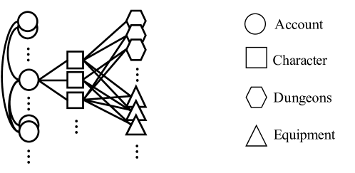
An entity, which is either account, character, dungeon, or equipment, becomes a node in the graph. A relationship between two entities forms an edge. There are four types of relationships: 1) (account - account), 2) (account - character), 3) (character - dungeon), and 4) (character - equipment) as shown in Fig. 3. Table 2 represents the number of edges between level-$1$ labels. The formed graph contains $249,455$ nodes and $7,885,487$ edges.

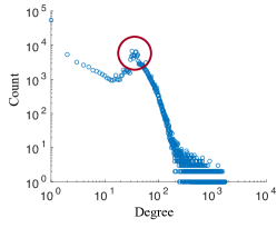
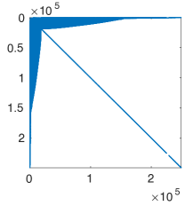
Fig. 4 shows the characteristics of the graph. The degree distributions of nodes for each level-1 label type are shown in Fig. 4(a). Note that degree distributions of all node types except character follow power-law. The degree distribution of character type nodes has a mode around the degrees $30\sim 40$ due to the following reasons: 1) the number of items a character can have is limited, and 2) the number of dungeons a character can visit is limited. Fig. 4(b) shows the degree distribution of all nodes. Even though there is a mode around the degrees $30\sim 40$, the graph shows a skewed degree distribution which is also verified in Fig. 4(c) which shows the reordered adjacency matrix from SlashBurn [4, 5] method. Note that a reordered adjacency matrix with a thin arrow shape like Fig. 4(c) means there are few high degree nodes in the graph which can be used for decomposing (or ‘shattering’) it [4].

3 Proposed Method: MDL Formulation

3.1 Overview

Our goal is to construct a concise summary of an MMORPG graph with hierarchical node labels. There are several challenges for the goal.

How can we summarize an MMORPG graph with a few key subgraphs (vocabularies)?

In designing an optimization objective for the summary, how can we incorporate hierarchical node labels?

Given a subgraph, how can we extract consistent substructures at different levels of hierarchy?

Our ideas to solve the challenges are as follows.

Exploiting Minimum Description Length (MDL) allows us to extract key structures (e.g., clique, star, bipartite core, etc.) from the MMORPG graph. We add the formulation for hierarchical labels while exploiting the formulation for structures used in VoG [1].

Considering label consistency of structures enables us to evaluate various structures in depth. We carefully formulate label consistency for each key structure.

Segmenting labels of an inconsistent structure from higher to lower levels generates consistent substructures. By determining segmentation at each level of the hierarchy, we extract pivotal structures from a heterogeneous graph.

In the following sections, we present the problem formulation for heterogeneous graph summarization based on the MDL, and how to design an optimization objective for the summary. We describe how to encode the connectivity of each structure, hierarchical labels, and errors. Then, we describe how to generate a summary of the graph based on the formulation. We describe subgraph generation, subgraph identification based on the encoding cost of structures, structure segmentation for label consistent structures by considering hierarchical labels, and model construction approaches. Table 3 shows the symbols used.

Table 3: Symbol description.

Symbol	Description
$G=(\mathcal{V},\mathcal{E})$	Graph with node set $\mathcal{V}$ and edge set $\mathcal{E}$
$\Omega$	Set of structure types
$st,ch$	Star & chain resp.
$fc,nc$	Full & near clique resp.
$bc,nb$	Full & near bipartite core resp.
$M$	Model
$\mathcal{M}$	Set of all possible models
$\mathbf{A}$	Adjacency matrix of $G$
$s$	Structure
$area(s)$	Edges of $G$ included in a structure $s$
$\mathbf{M}$	Approximate adjacency matrix of $\mathbf{A}$ induced by $M$
$\mathbf{E}$	Error matrix, $\mathbf{E}=\mathbf{M}\oplus\mathbf{A}$
$\oplus$	Exclusive OR
$L(G,M)$	# of bits to encode $G$ using $M$
$L(M)$	# of bits to encode model $M$
$L_{t}(s)$	# of bits to encode a structure $s$
$L_{a}(s)$	# of bits to encode node labels in a structure $s$
$|s|$	# of nodes in a structure $s$
$h$	# of levels
$\mathbf{E}^{+},\mathbf{E}^{-}$	Edges that were over-modeled and under-modeled resp.
$L(\mathbf{E}^{+}),L(\mathbf{E}^{-})$	Error encoding cost for $\mathbf{E}^{+}$ and $\mathbf{E}^{-}$ resp.
$L(\mathbf{E}^{a})$	Encoding cost for labeling error

3.2 MDL for Heterogeneous Graph Summarization with Hierarchical Labels

Minimum Description Length (MDL)  [6] is a model selection method where the best model $\hat{M}$ is the one that gives the best lossless compression:

$$\hat{M}=\operatorname*{arg\,min}_{M\in\mathcal{M}}{(L(M)+L(D|M))}$$

$M$ is a model, $\mathcal{M}$ is the set of all possible models, $D$ is the given data, $L(M)$ is the length in bits of $M$, and $L(D|M)$ is the length in bits of $D$ when encoded using $M$.

Our target model $M\in\mathcal{M}$ is an ordered list of graph structures each having a type from $\Omega$ [1]. Each structure $s\in M$ corresponds to a certain portion of the adjacency matrix $\mathbf{A}$ describing its node’s labels and interconnectivity; there may be overlapped nodes between different structures, but there is no edge overlap. Each node has a hierarchical label (e.g., Table 1).

Following the MDL principle, our method for transmitting the adjacency matrix $\mathbf{A}$ is the following. We 1) transmit model $M$, 2) induce the approximate adjacency matrix $\mathbf{M}$ of $\mathbf{A}$ by filling out the connectivity of each structure in $M$, 3) transmit the error $\mathbf{E}$ which is derived from taking the exclusive OR between $\mathbf{M}$ and $\mathbf{A}$ as MDL requires lossless encoding, and 4) transmit labeling error $\mathbf{E}^{a}$ which is the label information for nodes not included in model $M$. We opt for a model $M$ that minimizes the encoding length of model $M$, error $\mathbf{E}$, and labeling error $\mathbf{E}^{a}$. Our problem definition is as follows.

Problem 1 (Minimum Hierarchical Graph Description)

Given a heterogeneous graph $G$ with hierarchical labels on its nodes, its adjacency matrix $\mathbf{A}$, and set of structure types $\Omega$, find model $M$ that minimizes the total encoding length

$$L(G,M)=L(M)+L(\mathbf{E})+L(\mathbf{E}^{a})$$

where $\mathbf{E}$ is the error matrix derived by $\mathbf{E}=\mathbf{M}\oplus\mathbf{A}$, $\mathbf{M}$ is the approximate adjacency matrix of $\mathbf{A}$ induced by $M$, and $\mathbf{E}^{a}$ is the labeling error.

3.3 Encoding the Model

Full encoding length of a model $M\in\mathcal{M}$ is the following:

$$\begin{split}L(M)\;=\;&L_{\mathbb{N}}(|M|+1)+\log{|M|+|\Omega|-1\choose|\Omega|-1}\\ &+\sum_{s\in M}{(-\log(P(x(s)|M))+L_{t}(s)+L_{a}(s))}\end{split}$$ (1)

We encode 1) the total number of structures in $M$ using $L_{\mathbb{N}}$, Rissanen’s optimal encoding [7] for integers greater than $0$, 2) the number of structures for each type using an index over a weak number composition for each structure type $x\in\Omega$ in model $M$, and 3) the structure type $x(s)$ for each structure $s\in M$ using optimal prefix code, 4) its connectivity $L_{t}(s)$, and 5) the hierarchical labels $L_{a}(s)$ of nodes in it. The detailed encodings for connectivity and hierarchical labels are described in the following two sections, respectively.

3.4 Encoding Connectivity

We describe how to encode the connectivity of each structure $s$ and derive its cost $L_{t}(s)$.

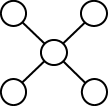
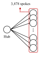
Stars. A star has a distinct characteristic of having a single ”hub” node surrounded by 2 or more ”spoke” nodes. We compute $L_{t}(st)$ of a star $st$ as follows, where $|st|$ is the number of nodes inside the star and $|\mathcal{V}|$ is the number of nodes inside the given graph $G$:

$$L_{t}(st)\;=\;L_{\mathbb{N}}(|st|-1)+\log|\mathcal{V}|+\log{|\mathcal{V}|-1\choose|st|-1}$$

We encode 1) the number of spokes in the star, 2) the index of the hub node over all $|\mathcal{V}|$ nodes, and 3) which nodes are included in the star’s spokes (spoke id).

Cliques. A full clique is a subset of vertices where every two distinct vertices are adjacent. We compute $L_{t}(fc)$ of a full clique $fc$ as follows, where $|fc|$ is the number of nodes inside the full clique:

$$L_{t}(fc)\;=\;L_{\mathbb{N}}(|fc|)+\log{|\mathcal{V}|\choose|fc|}$$

We encode 1) the number of nodes in the full clique, and 2) the index of a permutation to select $|fc|$ nodes out of $|\mathcal{V}|$ nodes.

Near cliques. A near clique has several missing edges from a full clique. We compute $L_{t}(nc)$ of a near clique $nc$ as follows:

$$\begin{split}L_{t}(nc)\;=\;&L_{\mathbb{N}}(|nc|)+\log{|\mathcal{V}|\choose|nc|}+\log(|area(nc)|)+||nc||\epsilon_{1}+||nc||^{\prime}\epsilon_{0}\end{split}$$

where $|nc|$ represents number of nodes inside $nc$, and $|area(nc)|$ is the number of edges in $nc$. We use $||nc||$ and $||nc||^{\prime}$, respectively, for the number of observable and non-observable edges in $nc$. $\epsilon_{1}$ and $\epsilon_{0}$ represent the lengths of the optimal prefix code for observable and non-observable edges, respectively.

$$\begin{aligned} \epsilon_{1}=-\log(\frac{||nc||}{||nc||+||nc||^{\prime}})\;\end{aligned}\;\;\begin{aligned} \;\epsilon_{0}=-\log(\frac{||nc||^{\prime}}{||nc||+||nc||^{\prime}})\end{aligned}$$

We encode 1) the number of nodes in the near clique, 2) the index of a permutation to select $|nc|$ nodes out of $|\mathcal{V}|$ nodes, 3) the number of edges, 4) the observable edges using the optimal prefix code, and 5) the non-observable edges.

Bipartite cores. A bipartite core consists of two sets of nodes $A$ and $B$ where edges exist only between the sets and not within them. A full bipartite core is a fully connected bipartite core. We compute $L_{t}(fb)$ of a full bipartite core $fb$ as follows.

$$L_{t}(fb)\;=\;L_{\mathbb{N}}(|A|)+L_{\mathbb{N}}(|B|)+\log{|\mathcal{V}|\choose|A|}+\log{|\mathcal{V}|\choose|B|}$$

where we encode 1) the number of nodes in node sets $A$ and $B$, and 2) ids of nodes in $A$ and $B$.

Near bipartite cores. A near bipartite core has several missing edges from a full bipartite core. We compute $L_{t}(nb)$ of a near bipartite core $nb$ as follows, similarly to a near clique:

$$\begin{split}L_{t}(nb)\;=\;&L_{\mathbb{N}}(|nb|)+\log{|\mathcal{V}|\choose|nb|}+\log(|area(nb)|)+||nb||\epsilon_{1}+||nb||^{\prime}\epsilon_{0}\end{split}$$

Chains. A chain is a sequence of nodes where each node is connected to the previous and the next node of it. We compute $L_{t}(ch)$ of a chain $ch$ as follows, where $|ch|$ is the number of nodes in $ch$:

$$L_{t}(ch)\;=\;L_{\mathbb{N}}(|ch|-1)+\sum_{i=1}^{|ch|}{\log{(|\mathcal{V}|-i+1)}}$$

We encode 1) the number of nodes in the chain, and 2) their ordered connectivity.

(a) Consistent star

(b) Role-consistent star

(c) Inconsistent star

Figure 5: Examples of label consistency in GSHL.

3.5 Encoding Hierarchical Labels

We describe how to encode the hierarchical labels for the nodes in a structure $s$ and derive its cost $L_{a}(s)$. Each node in our target graph has a hierarchical label: e.g., a character node may have a three-level hierarchical label ”character-tanker-blade master”. Furthermore, we assume that a different node may have a different depth of its label: e.g., a dungeon node may have only two-levels of hierarchy, like ”dungeon-advanced”. When transmitting a graph to the recipient, we assume that the recipient also knows how the hierarchical labels are structured. We start by formalizing label encoding costs for node labels in level-$k$, and describe a full label encoding cost $L_{a}(s)$ for hierarchical labels.

Base encoding. In level-$k$, the base label encoding cost of a structure $s$ is given by

$$\begin{split}L^{base}_{a}(s,k)=\sum_{m=1}^{|s|}{\log(l^{b}_{k,m})}\end{split}$$

where $|s|$ represents the number of nodes in the structure $s$. $l^{b}_{k,m}$ is the number of unique sibling labels for the level-$k$ label of the $m$-th node of the structure, where sibling labels of a label are those with the same upper level label (e.g. dealer, tanker, and buffer are sibling labels as they branch from character). For example, $l^{b}_{1,m}$, $l^{b}_{2,m}$, and $l^{b}_{3,m}$ are $4$, $3$ and $5$, respectively, when the labels of the $m$-th node are character-dealer-destroyer (see Table  1).

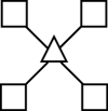
Label consistency. We define the label encoding costs for two special cases: 1) consistent structure, and 2) role-consistent structure. The two special cases allow us to reduce the label encoding cost. A consistent structure is the one containing only nodes with the same label, as shown in Fig. 5(a). A role-consistent structure is the one where nodes with the same role have the same label, as shown in Fig. 5(b). We define 4 roles in this work: 1) hub in a star structure, 2) spoke (neighbor of a star) in a star structure, 3) node belonging to the first set in a bipartite core, and 4) node belonging to the second set in a bipartite core. An inconsistent structure is the one that is neither consistent nor role-consistent, as shown in Fig. 5(c).

The label encoding cost for a consistent structure in level-$k$ is given by

$$L^{c}_{a}(s,k)=\log(l^{c}_{k})$$

where $l^{c}_{k}$ of a consistent structure is the number of unique sibling labels for the level-$k$ label. For a consistent structure, substituting $L^{c}_{a}(s,k)$ for $L^{base}_{a}(s,k)$ reduces the label encoding cost.

Next, the label encoding cost for a role-consistent structure in level-$k$ is given by

$$L^{rc}_{a}(s,k)=\log(l^{rc}_{k,1})+\log(l^{rc}_{k,2}-1)$$

where $l^{rc}_{k,1}$ and $l^{rc}_{k,2}$ of a role-consistent structure are the number of unique sibling labels for the level-$k$ labels of the two roles that a role-consistent structure can have, respectively. For a role-consistent structure, substituting $L^{rc}_{a}(s,k)$ for $L_{a}(s,k)$ reduces the label encoding cost.

Hierarchical label. We define the full encoding cost $L_{a}(s)$ for hierarchical labels as follows:

$$\begin{split}&L_{a}(s)\;=\;\log{|s|+l_{1}-1\choose l_{1}-1}+\sum_{i=1}^{h_{1}}{L^{c}_{a}(s,i)}+\sum_{j=h_{1}+1}^{h_{2}}{L^{rc}_{a}(s,j)}\\ &+\Big{(}\sum_{k=h_{2}+1}^{h}{L^{base}_{a}(s,k)}\Big{)}+2\log(h)\end{split}$$

where $h_{1}$ and $h_{2}$ mark the level in which consistent and role-consistent structures end, respectively; $h_{1}$ and $h_{2}$ are set to $0$ when consistent and role-consistent cases do not exist, respectively. $l_{1}$ is the number of unique labels in level-$1$ and $h$ is the number of levels. We encode 1) the number of each label at level-$1$ by using an index over a weak number composition, 2) consistent cases’ labels from level-$1$ to level-$h_{1}$, 3) role-consistent cases’ labels from level-$(h_{1}+1)$ to level-$h_{2}$, 4) remaining levels using the base encoding for inconsistent cases, and 5) $h_{1}$ and $h_{2}$. We consider the cases in the order of consistent, role-consistent, and inconsistent cases when moving from higher (e.g. level-1) to lower (e.g. level-3) levels.

3.6 Encoding Errors

Given the summary $M$ of $G$, it is vital to encode edges that are under or over-modeled by the model $M$ which we refer to as errors. Specifically, there are two types of errors to consider. The first type of error transpires in connectivity; if $area(s)$ is not identical to the regarding patch in $\mathbf{A}$, we encode the relevant errors. Another error type arises from labeling, where nodes that failed to be included in at least a structure lack label information.

3.6.1 Encoding Connectivity Errors

The encoding length $L(\mathbf{E})$ of connectivity error of a model is the following:

$$L(\mathbf{E})\;=\;L(\mathbf{E}^{+})+L(\mathbf{E}^{-})$$

$\mathbf{E}^{+}$ and $\mathbf{E}^{-}$ are edges that are over-modeled and under-modeled, respectively; $L(\mathbf{E}^{+})$ and $L(\mathbf{E}^{-})$ are the error encoding costs for $\mathbf{E}^{+}$ and $\mathbf{E}^{-}$, respectively. We encode $\mathbf{E}^{+}$ and $\mathbf{E}^{-}$ separately as they are likely to have different distributions. Note that we ignore the errors from near cliques and near bipartite cores as they have been encoded exactly. $L(\mathbf{E}^{+})$ and $L(\mathbf{E}^{-})$ are defined as follows.

$$L(\mathbf{E}^{+})\;=\;\log(|\mathbf{E}^{+}|)+||\mathbf{E}^{+}||\epsilon_{1}+||\mathbf{E}^{+}||^{\prime}\epsilon_{0}$$

$$L(\mathbf{E}^{-})\;=\;\log(|\mathbf{E}^{-}|)+||\mathbf{E}^{-}||\epsilon_{1}+||\mathbf{E}^{-}||^{\prime}\epsilon_{0}$$

We encode first the number of 1s in $\mathbf{E}^{+}$ or $\mathbf{E}^{-}$, and the 1s and 0s using the optimal prefix code.

3.6.2 Encoding Labeling Errors

We discuss encoding the labeling errors which occur for nodes that the model fails to cover, thus lacking the label information. Our idea is to include all considering nodes into one structure and apply base encoding for label encoding cost $L_{a}(s)$. Labeling error encoding cost $L(\mathbf{E}^{a})$ is the following:

$$\begin{split}L(\mathbf{E}^{a})\;=\;&\log{|en|+l_{1}-1\choose l_{1}-1}+\sum_{k=1}^{h}{{\sum_{m=1}^{|en|}\log(l^{b}_{k,m})}}\end{split}$$

where $|en|$ is the number of nodes in labeling error node set $en$, $l_{1}$ is the number of unique labels in level-$1$, and $l^{b}_{k,m}$ is the number of unique sibling labels for the level-$k$ label of the $m$-th node.

10:  A heterogeneous graph $G$ with hierarchical node labels 20:  Model $M$ 1:  Subgraph generation. Given the graph $G$, generate subgraphs using a graph decomposition method. 2:  Subgraph identification. For each subgraph obtained from step 1, we pick the structure which minimizes the local encoding cost of the subgraph. 3:  Structure segmentation. For each candidate structure, we segment it if the segmentation reduces the total encoding cost by considering the trade-off between the label encoding cost and the structure encoding cost. 4:  Model summary. We construct a model $M$ using summary approaches Vanilla, Top-k, and Benefit.

Algorithm 1 Graph Summarization with Hierarchical Labels

4 Proposed Method: Summary Generation

We present GSHL (Graph Summarization with Hierarchical Labels), our proposed summarization algorithm for heterogeneous graphs with hierarchical node labels. Algorithm 1 describes GSHL.

4.1 Subgraph Generation

We first decompose a given large graph into several subgraphs using a graph decomposition algorithm. We leverage SlashBurn [4] whose complexity is $O(T(m+n\log n))$ to generate subgraphs, where $m$ is the number of edges, $n$ is the number of nodes, and $T$ is the number of SlashBurn iterations. SlashBurn has been used for many graph tasks [8, 9, 10]; [1, 3] demonstrate that SlashBurn successfully decomposes real-world graphs for graph summarization. However, using other algorithms like SUBDUE [11] and BIGCLAM [12] is possible.

4.2 Subgraph Identification

For each generated subgraph, we find an appropriate structure in $\Omega$ to minimize the encoding cost. For each subgraph, we 1) compute the encoding cost for all structure types, 2) compare the encoding costs, and 3) encode the subgraph as the structure type with the minimum encoding cost. We assume that each subgraph corresponds to one structure among the six ones.

We determine the role of each node in a given subgraph to encode the subgraph as one of the structure types. For example, which node is the hub of a star? Which nodes are included in set A or set B of a bipartite core? How to determine the order of nodes in a chain? We determine the role of each node in the following ways.

Stars. We encode the highest-degree node of the subgraph as the hub, and the remaining nodes as the spokes.

Cliques. All nodes have the same structural role in a clique.

Bipartite cores. We determine which nodes are included in set A or set B using binary classification for bipartite cores [1, 3]. We add the highest degree nodes to set A, and its neighbors to set B. Then, we perform Fast Belief Propagation (FaBP) [13] to propagate classes and add nodes to set A or B.

Chains. We adopt a heuristic approach [1, 3] to encode a subgraph as a chain. We 1) randomly pick a node and find a farthest node using breadth first search (BFS), 2) set the discovered node as starting node $n_{s}$, 3) find a farthest node from $n_{s}$ and set it as end node $n_{e}$, and 4) designate the shortest path from $n_{s}$ to $n_{e}$ as the initial chain. Additionally, we extend the initial chain. We construct an induced subgraph by removing all nodes included in the initial chain except for $n_{e}$. We extend the chain by concatenating the shortest path from $n_{e}$ to a farthest node in the induced subgraph. We repeat the aforementioned process for $n_{s}$.

After obtaining the structures from a subgraph, we compute and compare the encoding costs of them. Given a subgraph $G^{\prime}$, we compute the local cost $L(M_{s})+L(\mathbf{E}_{M_{s}})$ [1, 3] to encode it as a structure $s$, where $M_{s}$ is the model consisting only of the subgraph $G^{\prime}$ encoded as $s$, and $\mathbf{E}_{M_{s}}$ is the error matrix derived by $\mathbf{E}_{M_{s}}=\mathbf{M}_{s}\oplus\mathbf{A}_{G^{\prime}}$. $\mathbf{A}_{G^{\prime}}$ is the adjacency matrix of the subgraph $G^{\prime}$ and $\mathbf{M}_{s}$ is the approximate adjacency matrix of $\mathbf{A}_{G^{\prime}}$ induced by $M_{s}$. Note that the labeling errors are ignored since nodes in a structure are connected and thus there are no uncovered nodes inside the structure. We compute $L(M_{s})$ by adding $L_{t}(s)$ and $L_{a}(s)$ (e.g., $L_{t}(st)+L_{a}(st)$ for $st$). The remaining terms except for $L_{t}(s)$ and $L_{a}(s)$ in Equation (1) are negligible, since $M_{s}$ consists only of the structure $s$. $L(\mathbf{E}_{M_{s}})$ is equal to $L(E^{+}_{M_{s}})+L(E^{-}_{M_{s}})$; $L(E^{+}_{M_{s}})$ and $L(E^{-}_{M_{s}})$ are the error encoding costs for $E^{+}_{M_{s}}$ and $E^{-}_{M_{s}}$, respectively, which are edges being over-modeled and under-modeled in the given subgraph $G^{\prime}$, respectively.

We add the best structure $s$ minimizing the local encoding cost $L(M_{s})+L(\mathbf{E}_{M_{s}})$ to the set $\mathcal{C}$ of structures.

Figure 6: GSHL chooses small segmented star structures in the right rather than a large inconsistent star in the left since the right ones minimize the encoding cost.

Figure 7: GSHL chooses the best structure with the minimum encoding cost among the 4 possible cases of segmentation in a bipartite core.

4.3 Structure Segmentation

We describe the segmentation of a structure considering hierarchical labels of nodes. The objective is to further reduce the label encoding cost for a structure considering the consistency of labels. Fig. 6 shows an example of comparison between a large inconsistent structure and small consistent structures. The inconsistent star graph in the left with 9 nodes has a low structure encoding cost, but a high label encoding cost. In contrast, the two decomposed star structures in the right have higher total structure encoding costs, but a lower total label encoding costs than the left case. We compare the total encoding costs before and after segmentation, and determine whether to segment or not by selecting the option leading to the minimum cost. We describe how to segment each structure, and how to extend the segmentation idea to hierarchical labels in the following two subsection, respectively.

4.3.1 Label Segmentation

We describe the segmentation of each structure in a level. We divide a structure into smaller structures of the same type only when the smaller structures provide a lower encoding cost.

Stars. We divide spokes of a star into two groups considering the consistency of labels, and construct two stars which have the same hub, but different spokes. We assign spoke nodes of the majority label to the first group and the remaining spoke nodes to the second group.

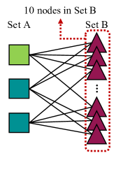
Bipartite cores. Bipartite cores have two sets of nodes. For each set, we search for the majority label in the set and divide the nodes of the set into the nodes with the majority label and the rest. As shown in Fig. 7, we consider $4$ cases depending on the segmentation for each set: 1) no segmentation, 2) segmenting only the first set, 3) segmenting only the second set, and 4) segmenting both sets. We choose the option with the minimum encoding cost among the 4 possible cases.

Cliques and chains. Contrary to star and bipartite core structures, all the nodes in cliques and chains have the same role. We first find the majority label, and then divide the structure into nodes of the majority label and the rest. We segment the given structure when the sum of the encoding costs of the two segmented structures is lower than that of the given structure.

4.3.2 Hierarchical Consideration

Given a structure with hierarchical labels, we segment the structure from higher to lower levels. For each level, we perform label segmentation to determine whether the structure should be segmented or not. Hierarchical label segmentation follows the following rules.

If a structure is consistent or role-consistent at the current level, the structure is challenged for label segmentation at the next lower level.

If an inconsistent structure is segmented and the current level is not the lowest the segmented structures are independently challenged for segmentation at the next lower level.

If an inconsistent structure is not segmented, we terminate the procedure and insert the structure in the set $\mathcal{C}$ of the candidate structures.

At the lowest level, we compare the encoding costs and insert the structure or the segmented structures in the set $\mathcal{C}$ of the candidate structures.

4.4 Model Summary

We construct the final model which summarizes the given heterogeneous graph by carefully selecting structures among the candidate structures $\mathcal{C}$. Finding the best model exactly by exploring all possible subsets of candidate structures is intractable. Thus we propose the following heuristics to choose a subset of candidate structures in a scalable way.

• Vanilla: All candidate structures are included in our summary, thus $M$ is equals to the set $C$ of the candidate structures.

• Top-k: We pick the top-$k$ structures by sorting the local encoding gains of candidate structures in descending order. A local encoding gain is the number of bits reduced by encoding a subgraph as a structure $x$.

• Benefit: We pick all structures whose local encoding gains are greater than zero.

GSHL uses the above approaches to finalize the model.

Table 4: Comparison of structures and costs of GSHL and the original graph. GSHL-Vanilla explains 99% of 7,885,487 edges using 25,740 structures. GSHL-Top-100 uses only 100 structures to explain 56% of edges. GSHL-Benefit uses 4,382 structures to explain 95% of edges.

		Description	Relative	Unexplained
Method	# of structures	cost (bits)	cost	edges
Original	$-$	$106,444,727$	$100\%$	$0\%$
GSHL-Vanilla	$25,740$	$52,124,308$	$49\%$	$1\%$
GSHL-Top-100	$100$	$75,781,149$	$71\%$	$56\%$
GSHL-Benefit	$4,382$	$52,237,349$	$49\%$	$5\%$

5 Experiment

We evaluate GSHL to answer the following questions:

• Graph summarization. How well does GSHL summarize the Blade & Soul graph?

• Discovery. What are the discovery results of analyzing Blade & Soul graph with GSHL?

• Finding similar users. How can we find similar users using the summary by GSHL?

• Scalability. How well does GSHL scale up in terms of the number of edges?

Table 5: Summarization results of Blade & Soul graph by GSHL. $st$, $fc$, $nc$, $bc$, $nb$, and $ch$ indicate star, full clique, near clique, bipartite core, near bipartite core, and chain, respectively.

st	fc	nc	bc	nb	ch
$22,787$	$21$	$-$	$-$	$2,467$	$465$

(a) GSHL-Vanilla

st	fc	nc	bc	nb	ch
$100$	$-$	$-$	$-$	$-$	$-$

(b) GSHL-Top-100

st	fc	nc	bc	nb	ch
$3,917$	$-$	$-$	$-$	$-$	$465$

(c) GSHL-Benefit

We use the Blade & Soul graph for experiments. We run experiments on a workstation with an Intel Xeon E5-2630 v4 @ 2.2GHz CPU and 512GB memory.

5.1 Graph Summarization (Q1)

We evaluate the description cost and edge coverage of Blade & Soul graph by GSHL. Our baseline is Original model where the original edges are encoded with $L(\mathbf{E}^{-})$ and the labels are encoded with $L(\mathbf{E}^{a})$.

Table 4 compares the number of structures, the description cost, and the ratio of unexplained edges by Original and the three proposed models (GSHL-Vanilla, GSHL-Top-100, and GSHL-Benefit). GSHL-Vanilla summarizes the given graph with only $49\%$ of the bits w.r.t. Original and explains all but $1\%$ of the edges which are not modeled by $M$. GSHL-Top-100 explains $44\%$ of the edges and summarizes the given graph with $71\%$ of the bits w.r.t. Original, while containing only $100$ structures out of $25,740$ structures. Each structure in GSHL-Top-100 contains a larger number of nodes and edges compared to the structures not included. Compared to GSHL-Vanilla, GSHL-Top-100 has fewer number of structures but a larger cost. GSHL-Benefit shows a reasonable balance between the description cost and the number of structures. Compared to GSHL-Vanilla, it has a similar description cost, but contains $5.9\times$ smaller number of structures.

(a) $st$

(b) $fc$

(c) $nb$

Figure 8: Meaningful structures from the summary. (a) $st$ (star) structure consisting only of accounts, where the hub node represents an influential account. (b) $fc$ (full clique) structure consisting of $8$ account nodes constituting a small clan. The $4$ accounts on the right possess characters which visited $6$ common dungeons. (c) $nb$ (near bipartite core) structure where a blade master and two wardens in set A (which are tankers) are equipped with several soul shields from set B, representing similar preferences for the three characters and similar properties for the $10$ soul shields.

5.2 Discovery (Q2)

We present the discovery results of Blade & Soul graph using GSHL.

5.2.1 Major Structures

How does GSHL summarize the Blade & Soul graph, and which structures can we discover? Table 5 shows the structures from our proposed methods GSHL-Vanilla, GSHL-Top-100, and GSHL-Benefit. Note that GSHL-Vanilla contains the most diverse structures including star, full cliques, near bipartite cores, and chains. GSHL-Top-100 contains only stars as they are the dominant structures when using SlashBurn for graph decomposition. GSHL-Benefit contains mainly stars, but it also contains several chains; it means that there are clear chain-like structures in the decomposed subgraphs.

5.2.2 Meaningful Structures

What interpretations can we make out of the summary? We report meaningful structures of Blade & Soul graph discovered by GSHL.

Popular dungeons and equipment. We observe that the hub node labels of star structures in GSHL-Top-100 mainly consist of popular dungeon and equipment nodes, surrounded only by character nodes. This is due to the nature of Blade & Soul where characters cooperate with other characters visiting various dungeons, while having various equipment.

Influential account. Fig. 8(a) shows a star structure consisting only of account nodes. The hub node is an influential account connected to $3,878$ other accounts.

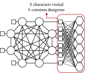
Small clan. Fig. 8(b) shows $8$ account nodes forming a full clique structure. The $4$ accounts on the right possess characters which visited $6$ common dungeons. This represents a small clan where the accounts play together frequently.

Near bipartite core of characters and equipment. Fig. 8(c) shows a bipartite core; a blade master and two wardens are tankers in set A, and they are equipped with several soul shields in set B. This indicates that all the three characters have the same preference for the equipment.

Segmented star. We analyze structures segmented by considering hierarchical labels. Fig. 1 shows that a large star structure whose hub is an equipment node with soul label is divided into three smaller star structures. The spokes of each star structure consist of: a) zen archers, b) dealers except for zen archers, and c) all jobs in tanker and buffer. This segmentation occurs since $37\%$ $(760/2041)$ of the spokes in the star structure are zen archers (out of the $11$ total jobs). Although any jobs can have this soul equipment, zen archers prefer this soul equipment the most.

5.3 Finding Similar Users (Q3)

How can we exploit the result of summarization for finding similar accounts in Blade & Soul? We measure account similarities as follows:

1. Matrix construction. Given the found structures, we first construct a node-structure matrix $\mathbf{B}$. The $(i,s)$-th element of the matrix $\mathbf{B}$ is set to a value $\gamma^{\alpha_{i,s}}$ where $\gamma$ is set to $0.7$ in this experiment and $\alpha_{i,s}$ is the minimum length of the shortest paths between account $i$ and nodes in structure $s$. If node $i$ is in structure $s$, $\alpha_{i,s}$ is set to $0$.

2. Randomized SVD for features. We compute a randomized SVD for the matrix $\mathbf{B}$ to obtain features of accounts.

3. Cosine similarity. We compute the cosine similarity of the two account feature vectors.

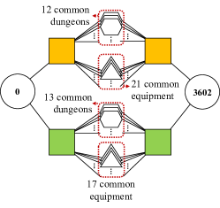
We pick a target account with id $0$, and find the two most similar accounts which have ids 3602 and 9. We observe that they share common characters, equipment, and often friends. Fig. 2(a) shows the relation of accounts 0 and 3602. Note that they have the characters with the same jobs (destroyer and blade master). The corresponding characters have common equipment and visited the same dungeons; e.g., the two destroyers have $21$ identical equipment, and visited $12$ identical dungeons. Fig. 2(b) shows the relation of accounts 0 and 9. We observe the similar patterns of characters and their related equipment and dungeons. They also share 18 common friends as well.

5.4 Scalability (Q4)

We measure the running times of GSHL varying the number of edges for scalability experiments. We generate 4 synthetic subgraphs using Forest Fire Sampling (FFS) [14], where (# of nodes, # of edges) are $(34203,78000)$, $(62339,246480)$, $(109764,780000)$, $(162759,2464800)$ and $(249455,7885487)$. Note that FFS enables generated subgraphs to follow the properties of real world graphs: heavy-tailed distributions, densification law, effective shrinking diameters [14]. As shown in Fig. 9, GSHL scales near-linearly with the number of edges.

6 Related Work

We present related works on four main categories: minimal description length, graph compression and summarization, hierarchical graph, and game data mining.

Minimal description length. MDL  [7] principle is a model selection method, where the best model is considered the one that gives the best lossless compression. Its use for compression  [15] is related to summarization and pattern discovery. GSHL exploits the MDL principle for summarizing a heterogeneous graph with hierarchical node labels.

Graph compression and summarization. Works like eigendecomposition  [16], modularity-based optimization  [17], and cross association  [18] find dense structures, such as cliques and bipartite cores. SUBDUE [11] discovers the best substructure that compresses a graph with node labels based on the MDL principle. Slashburn [4] reorders nodes of a graph to efficiently compress the graph by exploiting the characteristics of real-world graphs. [19] summarizes RDF graphs and [20] performs graph summarization for hashtag recommendation on social graphs. VoG [1] leverages the MDL principle to summarize a homogeneous graph with common structures. Shah et al. [3] propose TimeCrunch that extends VoG method for dynamic graphs. None of the above methods target a heterogeneous MMORPG graph, a heterogeneous graph with hierarchical labels, which GSHL focuses on.

Figure 9: GSHL provides near-linear scalability with regard to the number of edges.

Hierarchical graph. Hierarchical graphs have been studied for node embedding and classification. To effectively learn node embeddings in a graph, GNN methods use hierarchical structures. HGP-SL [21] and DiffPool [22] improve the performance of predicting unknown graph labels using hierarchical representations of graphs. StructureNet  [23] proposes a generator using hierarchical graph, which produces diverse and realistic mesh geometries. Zhang et al. [24] use hierarchical information of labels to improve multi-label classification performance. Wendt et al. [25] propose a hierarchical label propagation algorithm for document classification. Our work is the first one to summarize a heterogeneous graph with hierarchical labels. Unlike GSHL, none of the above methods address the problem of hierarchical graph summarization.

Game data mining. There have been several works for analyzing game data. Drachen et al. [26] analyze the behaviors of players in MMORPGs using a clustering approach. Bernardi [27] propose a bot detection algorithm by analyzing the behaviors of players. Yang et al. [28] cluster game players by analyzing their purchase records. Thompson et al. [29] analyze chat messages of players in StarCraft 2 using a lexicon-based approach. We represent a popular MMORPG data as a heterogeneous graph, and analyze the graph for summarization.

7 Conclusion

In this paper, we analyze a massive real-world MMORPG graph using hierarchical graph summarization. For the purpose, we propose GSHL, a novel graph summarization algorithm for a heterogeneous graph with hierarchical node labels. Based on the MDL principle, GSHL decomposes a heterogeneous graph into subgraphs, identifies each subgraph as a structure, segments each structure by considering hierarchical labels of its nodes, and summarizes the graph. Through extensive experiments on a large real-world MMORPG graph, we show that GSHL is a useful and scalable tool for graph summarization. Thanks to GSHL, we find key structures and similar users in the MMORPG graph.

References

- [1] D. Koutra, U. Kang, J. Vreeken, C. Faloutsos, VOG: summarizing and understanding large graphs, in: SDM, 2014, pp. 91–99.
- [2] D. Koutra, U. Kang, J. Vreeken, C. Faloutsos, Summarizing and understanding large graphs, Statistical Analysis and Data Mining: The ASA Data Science Journal 8 (3) (2015) 183–202.
- [3] N. Shah, D. Koutra, T. Zou, B. Gallagher, C. Faloutsos, Timecrunch: Interpretable dynamic graph summarization, in: SIGKDD, 2015, pp. 1055–1064.
- [4] U. Kang, C. Faloutsos, Beyond ’caveman communities’: Hubs and spokes for graph compression and mining, in: ICDM, 2011, pp. 300–309.
- [5] Y. Lim, U. Kang, C. Faloutsos, Slashburn: Graph compression and mining beyond caveman communities, IEEE Trans. Knowl. Data Eng. 26 (12) (2014) 3077–3089.
- [6] J. Rissanen, Modeling by shortest data description, Automatica 14 (5) (1978) 465 – 471.
- [7] J. Rissanen, A universal prior for integers and estimation by minimum description length, The Annals of statistics (1983) 416–431.
- [8] K. Shin, J. Jung, L. Sael, U. Kang, BEAR: block elimination approach for random walk with restart on large graphs, in: SIGMOD, 2015, pp. 1571–1585.
- [9] J. Jung, K. Shin, L. Sael, U. Kang, Random walk with restart on large graphs using block elimination, ACM Trans. Database Syst. 41 (2) (2016) 12.
- [10] J. Jung, N. Park, L. Sael, U. Kang, Bepi: Fast and memory-efficient method for billion-scale random walk with restart, in: SIGMOD, 2017, pp. 789–804.
- [11] D. J. Cook, L. B. Holder, Substructure discovery using minimum description length and background knowledge, J. Artif. Intell. Res. 1 (1994) 231–255.
- [12] J. Yang, J. Leskovec, Overlapping community detection at scale: a nonnegative matrix factorization approach, in: WSDM, 2013, pp. 587–596.
- [13] D. Koutra, T. Ke, U. Kang, D. H. Chau, H. K. Pao, C. Faloutsos, Unifying guilt-by-association approaches: Theorems and fast algorithms, in: ECML-PKDD, 2011, pp. 245–260.
- [14] J. Leskovec, J. M. Kleinberg, C. Faloutsos, Graphs over time: densification laws, shrinking diameters and possible explanations, in: SIGKDD, 2005, pp. 177–187.
- [15] C. Faloutsos, V. Megalooikonomou, On data mining, compression, and kolmogorov complexity, Data mining and knowledge discovery 15 (1) (2007) 3–20.
- [16] N. Shah, A. Beutel, B. Gallagher, C. Faloutsos, Spotting suspicious link behavior with fbox: An adversarial perspective, in: ICDM, 2014, pp. 959–964.
- [17] V. D. Blondel, J.-L. Guillaume, R. Lambiotte, E. Lefebvre, Fast unfolding of communities in large networks, Journal of statistical mechanics: theory and experiment 2008 (10) (2008) P10008.
- [18] D. Chakrabarti, S. Papadimitriou, D. S. Modha, C. Faloutsos, Fully automatic cross-associations, in: SIGKDD, 2004, pp. 79–88.
- [19] Š. Čebirić, F. Goasdoué, P. Guzewicz, I. Manolescu, Compact summaries of rich heterogeneous graphs.
- [20] M. Al-Dhelaan, H. Alhawasi, Graph summarization for hashtag recommendation, in: 3rd International Conference on Future Internet of Things and Cloud, FiCloud 2015, Rome, Italy, August 24-26, 2015, IEEE Computer Society, 2015, pp. 698–702.
- [21] Z. Zhang, J. Bu, M. Ester, J. Zhang, C. Yao, Z. Yu, C. Wang, Hierarchical graph pooling with structure learning, arXiv preprint arXiv:1911.05954.
- [22] Z. Ying, J. You, C. Morris, X. Ren, W. Hamilton, J. Leskovec, Hierarchical graph representation learning with differentiable pooling, in: Advances in Neural Information Processing Systems 31, 2018, pp. 4800–4810.
- [23] K. Mo, P. Guerrero, L. Yi, H. Su, P. Wonka, N. Mitra, L. J. Guibas, Structurenet: Hierarchical graph networks for 3d shape generation, arXiv preprint arXiv:1908.00575.
- [24] L. Zhang, S. K. Shah, I. A. Kakadiaris, Hierarchical multi-label classification using fully associative ensemble learning, Pattern Recognition 70 (2017) 89–103.
- [25] J. B. Wendt, M. Bendersky, L. G. Pueyo, V. Josifovski, B. Miklos, I. Krka, A. Saikia, J. Yang, M. Cartright, S. Ravi, Hierarchical label propagation and discovery for machine generated email, in: WSDM, 2016, pp. 317–326.
- [26] A. Drachen, R. Sifa, C. Bauckhage, C. Thurau, Guns, swords and data: Clustering of player behavior in computer games in the wild, in: CIG, 2012, pp. 163–170.
- [27] M. L. Bernardi, M. Cimitile, F. Martinelli, F. Mercaldo, A time series classification approach to game bot detection, in: WIMS, 2017, pp. 6:1–6:11.
- [28] W. Yang, G. Yang, T. Huang, L. Chen, Y. E. Liu, Whales, dolphins, or minnows? towards the player clustering in free online games based on purchasing behavior via data mining technique, in: Big Data, 2018, pp. 4101–4108.
- [29] J. J. Thompson, B. H. M. Leung, M. R. Blair, M. Taboada, Sentiment analysis of player chat messaging in the video game starcraft 2: Extending a lexicon-based model, Knowl.-Based Syst. 137 (2017) 149–162.