IIRC: Incremental Implicitly-Refined Classification

Abstract

We introduce the “Incremental Implicitly-Refined Classification (IIRC)” setup, an extension to the class incremental learning setup where the incoming batches of classes have two granularity levels. i.e., each sample could have a high-level (coarse) label like “bear” and a low-level (fine) label like “polar bear”. Only one label is provided at a time, and the model has to figure out the other label if it has already learned it. This setup is more aligned with real-life scenarios, where a learner usually interacts with the same family of entities multiple times, discovers more granularity about them, while still trying not to forget previous knowledge. Moreover, this setup enables evaluating models for some important lifelong learning challenges that cannot be easily addressed under the existing setups. These challenges can be motivated by the example ”if a model was trained on the class bear in one task and on polar bear in another task, will it forget the concept of bear, will it rightfully infer that a polar bear is still a bear? and will it wrongfully associate the label of polar bear to other breeds of bear?”. We develop a standardized benchmark that enables evaluating models on the IIRC setup. We evaluate several state-of-the-art lifelong learning algorithms and highlight their strengths and limitations. For example, distillation-based methods perform relatively well but are prone to incorrectly predicting too many labels per image. We hope that the proposed setup, along with the benchmark, would provide a meaningful problem setting to the practitioners.

1 Introduction

Figure 1: Humans incrementally accumulate knowledge over time. They encounter new entities and discover new information about existing entities. In this process, they associate new labels with entities and refine or update their existing labels, while ensuring the accumulated knowledge is coherent.

Figure 2: IIRC setup showing how the model expands its knowledge and associates and re-associates labels over time. The top right label shows the label model sees during training, and the bottom label (annotated as “Target”) is the one that model should predict during evaluation. The right bottom panel for each task shows the set classes that model is evaluated on and the dashed line shows different tasks.

Deep learning algorithms have led to transformational breakthroughs in computer vision [12, 17], natural language processing [19, 50], speech processing [3, 5], reinforcement learning [36, 44], robotics [16, 1], recommendation systems [11, 18] etc. On several tasks, deep learning models have either matched or surpassed human performance. However, such super-human performance is still limited to some very narrow and well-defined setups. Moreover, humans can continually learn and accumulate knowledge over their lifetime, while the current learning algorithms are known to suffer from several challenges when training over a sequence of tasks [33, 15, 8, 45]. These challenges are broadly studied under the domain of Lifelong Learning [47], also called Incremental Learning [42], Continual Learning [48], and Never Ending Learning [35]. In the general lifelong learning setup, the model experiences new knowledge, in terms of new tasks, from the same domain or different domains. The model is expected to learn and solve new tasks while retaining useful knowledge from previous tasks.

There are two popular paradigms in lifelong learning [49]: i) task incremental learning, where the model has access to a task delimiter (say a task id), which distinguish between tasks. Models for this setup are generally multi-headed, where there exists a separate classification layer for each task. ii) class incremental learning, where the model does not have access to a task delimiter, so it needs to discriminate between all classes from all tasks at inference time. Therefore, models developed for this paradigm are generally single-headed. The class incremental setup is more closely aligned with the real-life scenarios and is more challenging than the task incremental scenario.

Several useful benchmarks have been proposed for evaluating models in the lifelong learning setting [4, 25]. While useful for measuring high-level aggregate quantities, these benchmarks take a narrow and limited view on the broad problem of lifelong learning. One common assumption that many class incremental setups make is “information about a given sample (say label) can not change across tasks”. For example, an image of a bear is always labeled as “bear”, no matter how much knowledge the model has acquired.

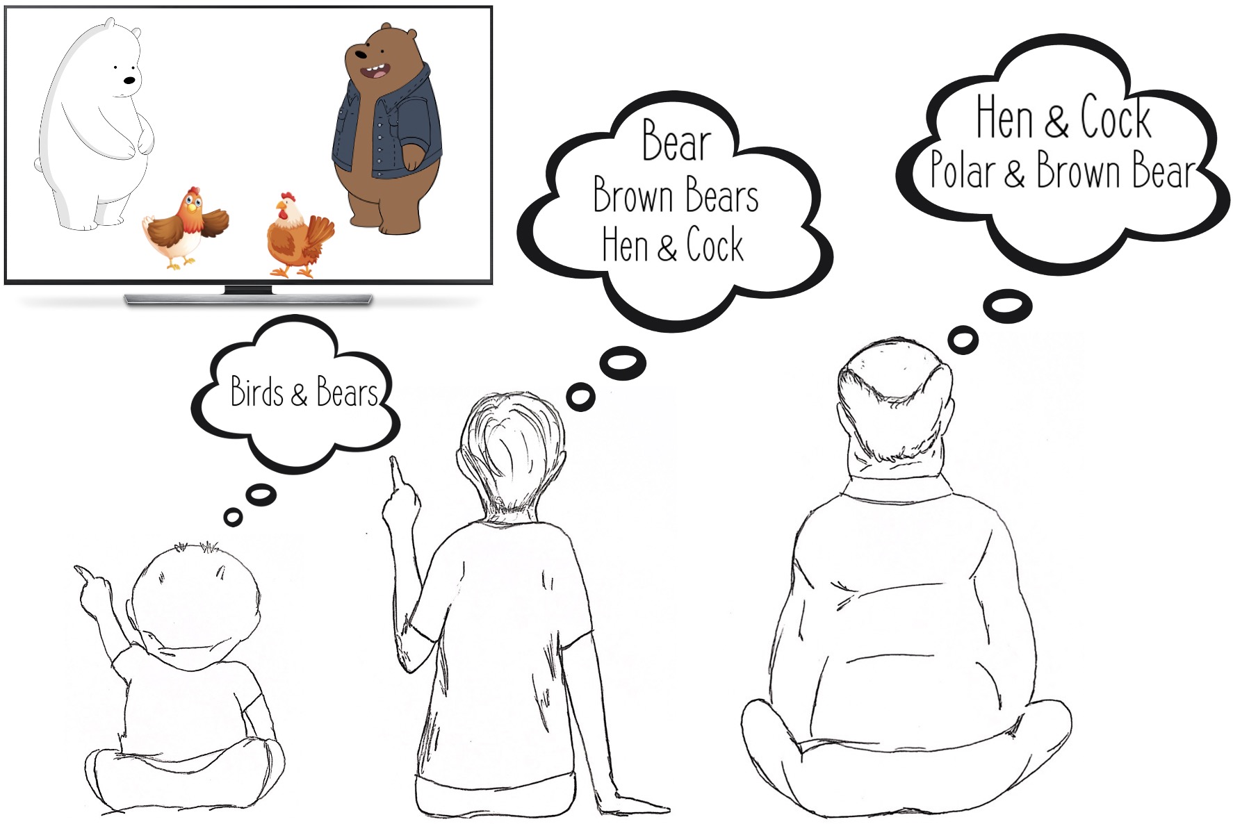
While this assumption appears to be “obviously correct” in the context of the supervised learning paradigm (where each sample generally has a fixed label), the assumption is not always satisfied in real-life scenarios. We often interact with the same entities multiple times and discover new information about them. Instead of invalidating the previous knowledge or outright rejecting the new information, we refine our previous knowledge using the new information. Figure 1 illustrates an example where a child may recognize all bears as “bear” (and hence label them as “bear”). However, while growing up, they may hear different kinds of bear being called by different names, and so they update their knowledge as: “Some bears are brown bears, some bears are polar bears, and other bears are just bears. Brown bears and polar bears are both still bears but they are distinct”. This does not mean that their previous knowledge was wrong (or that previous label “bear” was “incorrect”), but they have discovered new information about an entity and have coherently updated their knowledge. This is the general scheme of learning in humans.

A concrete instantiation of this learning problem is that two similar or even identical input samples have two different labels across two different tasks. We would want the model to learn the new label, associate it with the old label without forgetting the old label. Evaluating lifelong learning models for these capabilities is generally outside the scope of existing benchmarks. We propose the Incremental Implicitly-Refined Classification (IIRC) setup to fulfill this gap. We adapt the publicly available CIFAR100 and ImageNet datasets to create a benchmark instance for the IIRC setup and evaluate several well-known algorithms on the benchmark. Our goal is not to develop a new state-of-the-art model but to surface the challenges posed by the IIRC setup.

The main contributions of our work are as follows:

1. We propose the Incremental Implicitly-Refined Classification (IIRC) setup, where the model starts training with some coarse, high-level classes and observes new, fine-grained classes as it trains over new tasks. During the lifetime of the model, it may encounter a new sample or an old sample with a fine-grained label.

2. We provide a standardized benchmark to evaluate a lifelong model in the IIRC setup. We adapt the commonly used ImageNet and CIFAR datasets, and provide the benchmark setup compatible with several major deep learning frameworks (PyTorch, Tensorflow, and Jax).

3. We evaluate well-known lifelong learning algorithms on the benchmark and highlight their strengths and limitations, while ensuring that the models are compared in a fair and standardized setup.

2 Incremental Implicitly-Refined Classification (IIRC)

While class incremental learning is a challenging and close-to-real-life formulation of the lifelong learning setup, most existing benchmarks do not explore the full breadth of the complexity. They tend to over-focus on catastrophic forgetting (which is indeed an essential aspect) at the expense of several other unique challenges to the class incremental learning. In this work, we highlight those challenges and propose the Incremental Implicitly-Refined Classification (IIRC) setting, an extension of the class incremental learning setting, that enables us to study these under-explored challenges, along with the other well-known challenges like catastrophic forgetting. We provide an instantiation of the setup, in the form of a benchmark, and evaluate several well-known lifelong learning algorithms on it.

2.1 Under-explored challenges in class incremental learning setting

In class incremental learning, the model encounters new classes as it trains over new tasks. The nature of the class distributions and the relationship between classes (across tasks) can lead to several interesting challenges for the learning model: If the model is trained on a high-level label (say “bear”) in the initial task and then trained on a low-level label, which is a refined category of the previous label (say “polar bear”), what kind of associations will the model learn and what associations will it forget? Will the model generalize and label the images of polar bear as both “bear” and “polar bear”? Will the model catastrophically forget the concept of “bear”? Will the model infer the spurious correlation: “all bears are polar bears”? What happens if the model sees different labels (at different levels of granularity) for the same sample (across different tasks)? Does the model remember the latest label or the oldest label or does it remember all the labels? These challenges can not be trivially overcome by removing restrictions on memory or replay buffer capacity (as we show in Section 6).

2.2 Terminology

We describe the terminology used in the paper with the help of an example. As shown in Figure 2, at the start, the model trains on data corresponding to classes “bear”, “bus” and “dog”. Training the model on data corresponding to these three classes is the first task. After some time, a new set of classes (“polar bear”, “lamp” and “whippet”) is encountered, forming the second task. Since “whippet” is a type of “dog”, it is referred as the subclass, while “dog” is refereed as the superclass. The “dog-whippet” pair is referred to as the superclass-subclass pair. Note that not all classes have a superclass (example “lamp”). We refer to these classes as subclasses as well, though they do not have any superclasses. When training the model on an example of a “whippet”, we may provide only “whippet” as the supervised learning label. This setup is referred to as the incomplete information setup, where if a task sample has two labels, only the label that belongs to the current task is provided. Alternatively, we may provide both “whippet” and “dog” as the supervised learning labels. This setup is referred as the complete information setup, where if a task sample has two labels, labels that belong to the current and previous tasks are provided. Note that majority of our experiments are performed in the incomplete information setup as that is closer to the real life setup, requiring the model to recall the previous knowledge when it encounters some new information about a known entity. We want to emphasize that the use of the word task in our setup refers to the arrival of a new batch of classes for the model to train on in a single-head setting, and so it is different from it’s use to indicate a distinct classification head in the task incremental learning.

As the model is usually trained in an incomplete information setup, it would need access to a validation set to monitor the progress in training that is still an incomplete information set, otherwise there would be some sort of labels leakage. On the other hand, after training on a specific task, the model has to be be evaluated on a complete information set, hence a complete information validation set is needed to be used during the process of model development and tweaking, so as to not overfit on the test set. We provide both in the benchmark, where we call the first one the in-task validation set, while the latter one the post-task validation set.

2.3 Setup

We describe the high-level design of the IIRC setup (for a visual illustration, see Figure 2). We have access to a series of $N$ tasks denoted as $T_{1},\cdots,T_{N}$. Each task comprises of three collections of datasets, for training, validation and testing. Each sample can have one or two labels associated with it. In the case of two labels, one label is a subclass and the other label is a superclass. For any superclass-subclass pair, the superclass is always introduced in an earlier task, with the intuition that a high-level label should be relatively easier to learn. Moreover, the number of samples for a superclass is always more than the number of samples for a subclass (it increases with the number of subclasses, up to a limit). During training, we always follow the incomplete information setup. During the first task, only a subset of superclasses (and no sublcasses) are used to train the model. The first task has more classes (and samples), as compared to the other tasks and it can be seen as a kind of pretraining task. The subsequent tasks have a mix of superclasses and subclasses. During the training phase, the model is evaluated on the in-task validation set (with incomplete information), and during the evaluation phase, the model is evaluated on the post-task validation set and the test set (both with complete information).

3 Related Work

Lifelong Learning is a broad, multi-disciplinary, and expansive research domain with several synonyms: Incremental Learning [42], Continual Learning [48], and Never Ending Learning [35]. One dimension for organizing the existing literature is whether the model has access to explicit task delimiters or not, where the former case is referred to as task incremental learning, and the latter case, which is closely related to our setup IIRC, is referred to as class incremental learning.

In terms of learning methods, there are three main approaches [23]: i) replay based, ii) regularization based, and iii) parameter isolation methods. Parameter isolation methods tend to be computationally expensive and require access to a task identifier, making them a good fit for the task incremental setup. Prominent works that follow this approach include Piggyback [29], PackNet [30], HAT [43], TFM [32], DAN [40], PathNet [14]. The replay and regularization based approaches can be used with both task and class incremental setups, however, replay based approaches usually perform better in the class incremental setup [31]. Among the regularization based approaches, LwF [24] uses finetuning with distillation. LwM [13] improves LwF by adding an attention loss. MAS [2], EWC [21], SI [52] and RWalk [8] estimate the importance of network parameters, and penalize changes to important ones. As for the replay based approaches, iCaRL [38] is considered an important baseline in the field. iCaRL selects exemplars for the replay buffer using herding strategy, and alleviates catastrophic forgetting by using distillation loss during training, and using a nearest-mean-of-exemplars classifier during inference. EEIL [7] modifies iCaRL by learning the feature extractor and the classifier jointly in an end to end manner. LUCIR [20] applies the distillation loss on the normalized latent space rather than the output space, proposes to replace the standard softmax layer with a cosine normalization layer, and uses a margin ranking loss to ensure a large margin between the old and new classes. Other works include LGM [37], IL2M [6], BIC [51], and ER [39]. GEM is another replay-based method, which solves a constrained optimization problem. It uses the replay buffer to constrain the gradients on the current task so that the loss on the previous tasks does not increase. A-GEM [9] improves over GEM by relaxing some of the constraints, and hence increasing the efficiency, while retaining the performance. Finally, [10] shows that vanilla experience replay, where the model simply trains on the replay buffer along with the new task data, is by itself a very strong baseline. In this work, we include variants of iCaRL, LUCIR, A-Gem, and vanilla experience replay as baselines.

We propose a benchmark for evaluating a model’s performance in the IIRC setup, as having a realistic, standardized, and large-scale benchmark helps provide a fair and reproducible comparison for the different approaches. Existing efforts for benchmarking the existing lifelong learning setups include CORe50 benchmark [25], and  [4] that proposes a benchmark for continual few-shot learning.

Our work is also related to knowledge (or concept) drift, where the statistical properties of the data changes over time and old knowledge can become “irrelevant”  [28, 27]. Unlike those works, we focus on learning new associations and updating existing associations as new tasks are learnt. As the model acquires new knowledge, the old knowledge does not become ‘irrelevant”. Recently, BREEDS [41] proposed a benchmark to evaluate model’s generalization capabilities in the context of subpopulation shift. Specifically, they define a hierarchy and train the model on samples corresponding to some subpopulations (e.g. “poodles” and “terriers” are subpopulations of “dogs”). The model is then evaluated on samples from an unseen subpopulation. e.g. it should label “dalmatians” as “dogs”. While at a quick glance, IIRC might appear similar to BREEDS, there are several differences. IIRC focuses on the lifelong learning paradigm while BREEDS focuses on generalization. Moreover, the training and evaluation setups are also different. If we were to extend the dogs example to IIRC, the model may first train on some examples of “poodles“ and “terriers” (labeled as “dogs”). In the next task, it may train on some exampled of “poodles” (labeled as “poodles”). When the model is evaluated on both tasks, it should predict both labels (“poodles” and “dogs”) for the images of poodles.

4 Benchmark

4.1 Dataset

We use two popular computer vision datasets in our benchmark - ImageNet [12] and CIFAR100 [22]. For both the datasets, we create a two-level hierarchy of class labels, where each label starts as a leaf-node and similar labels are assigned a common parent. The leaf-nodes are the subclasses and the parent-nodes are the super-classes. Some of the subclasses do not have a corresponding superclass, so as to enrich the setup and make it more realistic. While the datasets come with a pre-defined hierarchy (e.g. ImageNet follow the WordNet hierarchy), we develop a new hierarchy as the existing hierarchy focuses more on the semantics of the labels and less on the visual similarity (e.g, “sliding door” and “fence” are both grouped under “barriers”). We refer to these adapted datasets as IIRC-ImageNet and IIRC-CIFAR.

Figure 3: The distribution of the number of subclasses per superclass on IIRC-Imagenet.

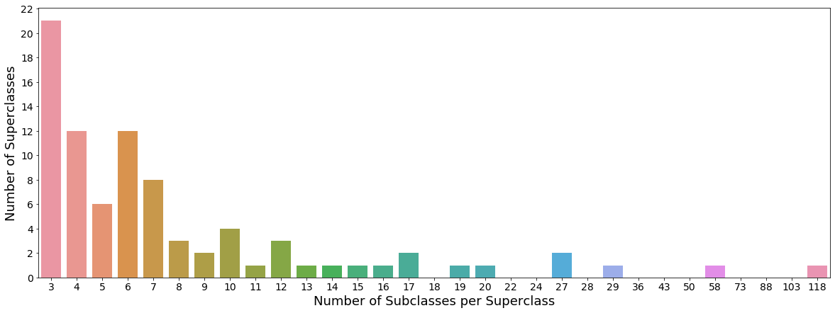
In IIRC-CIFAR, each superclass has similar number of subclasses (four to eight). However, the sub-class distribution for IIRC-ImageNet is very skewed (Figure 3) and number of sublcasses varies from 3 to 118. We explicitly decided not to fix this imbalance to ensure that visually similar classes are grouped together. Moreover, in the real life, not all classes are observed at the same frequency, making our setup more realistic. More statistics and the full class hierarchies for both IIRC-ImageNet and IIRC-CIFAR are provided in Appendix-C and G.

As mentioned in Section 2, we use two validation sets - one with incomplete information (for model selection and monitoring per-task performance) and one with complete information (for the model evaluation after each task). Each validation dataset comprises 10% of the training data for CIFAR, and 4% of the training data for ImageNet, and is fixed through all the runs. Some aggregate information about the splits is provided in Table 1 in Appendix.

Since we are creating the class hierarchy, superclasses do not have any samples assigned to them. For the training set and the in-task validation set, we assign 40% of samples from each subclass to its superclass, while retaining 80% of the samples for the subclass. This means that subclass-superclass pairs share about 20% of the samples or, for 20% of the cases, the model observes the same sample with different labels (across different tasks). Since some superclasses have an extremely large number of subclasses, we limit the total number of samples in a superclass. A superclass with more than eight subclasses, uses $\frac{8}{\text{number of subclasses}}\times 40\%$ of samples from its subclasses. We provide the pseudo code for the dataloader in Appendix F.

Now that we have a dataset with superclasses and subclasses, and with samples for both kind of classes, the tasks are created as follows: The first task is always the largest task with 63 superclasses for IIRC-ImageNet and 10 superclasses for IIRC-CIFAR. In the supsequent tasks, each new task introduces 30 classes for IIRC-ImageNet and 5 classes for IIRC-CIFAR. Recall that each task introduces a mix of superclasses and subclasses. IIRC-ImageNet has a total of 35 tasks, while IIRC-CIFAR has a total of 22 tasks. Since the order of classes can have a bearing on the models’ evaluation, we create 5 preset class orders (called task configurations) for IIRC-ImageNet and 10 task configurations for IIRC-CIFAR, and report the average (and standard deviation) of the performance on these configurations.

Finally, we acknowledge that while IIRC-ImageNet provides interesting challenges in terms of data diversity, training on the dataset could be difficult and time consuming. Hence, we provide a shorter, lighter version which has just ten tasks (with five tasks configurations). We shall call the original version IIRC-ImageNet-full, and the lighter version IIRC-ImageNet-lite, while referring to both collectively as IIRC-ImageNet. Although we do not recommend the use of this lighter version for benchmarking the model performance, we hope that it will make it easier for others to perform quick, debugging experiments. We report all the metrics on IIRC-ImageNet-lite as well.

4.2 Metrics

Figure 4: Average performance using the precision-weighted Jaccard Similarity. (left) IIRC-Imagenet-lite and (right) IIRC-Imagenet-full. We run experiments on five different task configurations and report the mean and standard deviation.

Figure 5: Average performance on IIRC-CIFAR. We run experiments on ten different task configurations and report the mean and standard deviation.

Most lifelong learning benchmarks operate in the single-label classification setup, making accuracy the appropriate metric. In our setup, the model should be able to predict multiple labels for each sample, even if those labels are seen across different tasks. We considered using the Exact-Match Ratio ($MR$) metric [46], a multi-label extension of the accuracy metric. $MR$ is defined as $\frac{1}{n}\sum_{i=1}^{n}I(Y_{i}==\hat{Y}_{i})$ where $I$ is the indicator function, $\hat{Y}_{i}$ are the set of (model) predictions for the $i_{th}$ sample, $Y_{i}$ are the ground truth labels, and $n$ is the total number of samples. One limitation is that it does not differentiate between partially incorrect predictions and completely incorrect predictions.

Another popular metric (for multi-label classification) is the Jaccard similarity($JS$), also called “intersection over union”[46]. $JS$ is defined as $\frac{1}{n}\sum_{i=1}^{n}\frac{|Y_{i}\cap\hat{Y}_{i}|}{|Y_{i}\cup\hat{Y}_{i}|}$. To further penalize the imprecise models, we weight the Jaccard similarity by the per sample precision (i.e., the ratio of true positives over the sum of true positives and false positives). We refer to this metric as the precision-weighted Jaccard similarity (pw-JS).

We measure the performance of a model on task $k$ after training on task $j$ using the precision-weighted Jaccard similarity, denoted $R_{jk}$, as follow:

$$R_{jk}=\frac{1}{n_{k}}\sum_{i=1}^{n_{k}}\frac{|Y_{ki}\cap\hat{Y}_{ki}|}{|Y_{ki}\cup\hat{Y}_{ki}|}\times\frac{|Y_{ki}\cap\hat{Y}_{ki}|}{|\hat{Y}_{ki}|}\,,$$ (1)

where ($j\geq k$), $\hat{Y}_{ki}$ is the set of (model) predictions for the $i_{th}$ sample in the $k_{th}$ task, $Y_{ki}$ are the ground truth labels, and $n_{k}$ is number of samples in the task. $R_{jk}$ can be used as a proxy for the model’s performance on the $k^{th}$ task as it trains on more tasks (i.e. as the $j$ increases).

We evaluate the overall performance of the model after training till the task $j$, as the average precision-weighted Jaccard similarity over all the classes that the model has encountered so far. Note that during this evaluation, the model has to predict all the correct labels for a given sample, even if the labels were seen across different tasks (i.e. the evaluation is performed in the complete information setup). We denote this metric as $R_{j}$ and computed it as follow:

$$R_{j}=\frac{1}{n}\sum_{i=1}^{n}\frac{|Y_{i}\cap\hat{Y}_{i}|}{|Y_{i}\cup\hat{Y}_{i}|}\times\frac{|Y_{i}\cap\hat{Y}_{i}|}{|\hat{Y}_{i}|}\,,$$ (2)

where $n$ is the total number of evaluation samples for all the tasks seen so far.

5 Baselines

Figure 6: Per task performance over the test samples of a specific task $j$, after training on that task ($R_{jj}$ using Equation 1). (left) IIRC-Imagenet-full and (right) IIRC-CIFAR.

We evaluate several well-known lifelong learning baselines. We also consider two training setups where the model has access to all the labels for a given sample (complete information setup): i) joint where the model is jointly trained on all the classes/tasks at once and ii) incremental joint where as the model trains across tasks, it has access to all the data from the previous tasks in a complete information setup. In the Finetune baseline, the model continues training on new batches of classes without using any replay buffer. Vanilla Experience Replay (ER) method finetunes the model on new classes, while keeping some older samples in the replay buffer and rehearsing on them. Experience Replay with infinite buffer (ER-infinite) is similar to incremental joint, but in incomplete information setup as in ER. This means that if a new label is introduced that applies to an old sample, the target for that sample will be updated with that new label in the incremental joint baseline but not in the ER-infinte baseline . We also have A-GEM [9] that is a constrained optimization method in the replay-based methods category. It provides an efficient version of GEM [26] by minimizing the average memory loss over the previous tasks at every training step. Another baseline is iCaRL [38] that proposed using the exemplar rehearsal along with a distillation loss. LUCIR [20] is a replay-based class incremental method that alleviates the catastrophic forgetting and the negative effect of the imbalance between the older and newer classes. More details about the baselines can be found in Appendix-B.

5.1 Model Adaptations

The earlier-stated baselines were proposed for the single label class incremental setup, while IIRC setup requires the model to be able to make multi-label predictions. Therefore, some changes have to be applied to the different models to make them applicable in the IIRC setup. To this end, we use the binary cross-entropy loss (BCE) as the classification loss. This loss is averaged by the number of observed classes so that it doesn’t increase as the number of classes increases during training. During prediction, a sigmoid activation is used and classes with values above 0.5 are considered the predicted labels. Using the nearest-mean-classifier strategy for classifying samples in iCaRL is not feasible for our setting, as the model should be able to predict a variable number of labels. To overcome this issue, we use the output of the classification layer, which was used during training, and call this variant as iCaRL-CNN. We further consider a variant of iCaRL-CNN, called iCaRL-norm, which uses cosine normalization in the last layer.  [20] suggests that using this normalization improves the performance in the context of incremental learning. Hence the classification score is calculated as:

$$p_{i}(x)=\sigma(\eta\langle\bar{\theta}_{i}\,,\bar{f}(x)\rangle)\,,$$ (3)

where $\sigma$ is the sigmoid function, $\bar{\theta}_{i}$ are the normalized weights of the last layer that correspond to label $i$, and $\bar{f}(x)$ is the output of the last hidden layer for sample $x$. $\eta$ is a learnable scalar that controls the peakiness of the sigmoid. It is important to have $\eta$ since $\langle\bar{\theta}_{i}\,,\bar{f}(x)\rangle$ is restricted to $[-1,1]$. We can either fix the $\eta$ or consider it as a learnable parameter. We observed that learning $\eta$ works better in practice.

(a) ground truth

(b) ER

(c) iCaRL-norm

(d) LUCIR

Figure 7: Confusion matrix after training on task 10 of IIRC-CIFAR. The y-axis is the correct label (or one of the correct labels). The x-axis is the model predicted labels. Labels are arranged by their order of introduction. Only 25 labels are shown for better visibility. See Appendix D.2 for the full resolution figures with labels.

6 Experiments

We design our experimental setup to surface challenges that lifelong learning algorithms face when operating in the IIRC setup. Our goal is neither to develop a new state-of-the-art model nor to rank existing models. We aim to highlight the strengths and weakness of the dominant lifelong learning algorithms, with the hope that this analysis will spur new research directions in the field. We use the ResNet architecture [17], with ResNet-50 for IIRC-ImageNet and reduced ResNet-32 for IIRC-CIFAR. Additional implementation details and hyperparameters can be found in Section A in the Appendix. Data used to plot the figures is provided in Appendix H for easier future comparisons.

6.1 Results and Discussion

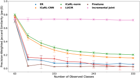
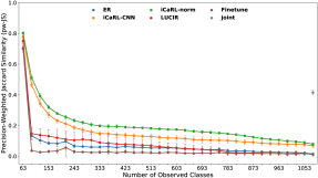
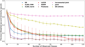
We start by analyzing how well does the model perform over all the observed classes as it encounters new classes. Specifically, as the model finishes training on the $j^{th}$ task, we report the average performance $R_{j}$, as measured by the pw-JS metric using Equation 2, over the evaluation set of all the tasks the model has seen so far (Figures 4 and 5). Recall that when computing $R_{j}$, the model has to predict all the correct labels for a given sample, even if the labels were seen across different tasks. This makes $R_{j}$ a challenging metric as the model can not achieve a good performance just by memorizing the older labels, but it has to learn the relationship between labels.

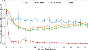
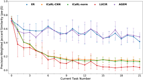
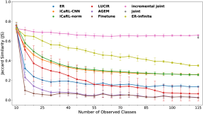
In Figures 4 and 5, we observe that the iCaRL-CNN and iCaRL-norm models perform relatively better than the other methods, with iCaRL-norm having the edge in the case of IIRC-ImageNet. However, this trend does not describe the full picture, as the iCaRL family of models is usually predicting more labels (some of which are incorrect). This behaviour can be observed for the IIRC-CIFAR setup in Figure 7(c) where they tend to predict too many labels incorrectly, which penalize their performance with respect to the PW-JS metric as opposed to the JS metric (see Figure A.8 in the Appendix). We also note that A-GEM model performs poorly in the case of IIRC-CIFAR, even when compared to vanilla ER, and hence we didn’t run A-GEM on IIRC-Imagenet.

One thing to notice in Figure 5, is the discrepancy between the performance of the ER-infinite baseline and the incremental joint baseline. Recall from section 5 that although both baselines don’t discard previous tasks samples, incremental joint is using the complete information setup, and hence it updates the older samples with the newly learned labels if applicable, while ER-infinite is using the incomplete information setup. This result tells us that dealing with the memory constraint is not sufficient by itself for a model to be able to perform well in the IIRC setup.

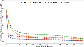
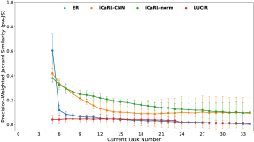
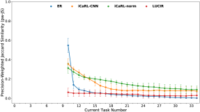
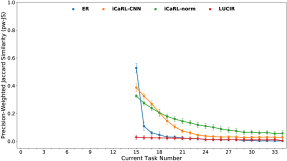
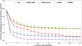
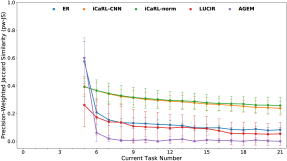
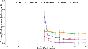
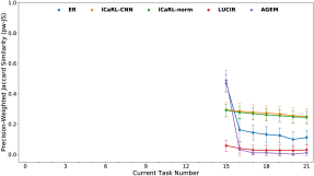
In lifelong learning setups, the model should retain the previous knowledge as it learns new tasks. Our setup is even more challenging because the model should not only retain previous knowledge, but it should incorporate the new labels as well in this previous knowledge. In Figure A.9 and A.10, we track how well the model performs on a specific task, as it is trained on subsequent tasks. Unlike the standard class incremental setup, the model should be able to re-associate labels across different tasks to keep performing well on a previous task. The key takeaway is that, while the baselines are generally expected to reasonably alleviate catastrophic forgetting, their performance degrades rapidly as the model trains on more tasks. ER’s poor performance may be accounted for by two hypothesis: i) The model is trained on a higher fraction of samples per class for classes that belong to the current task, than those of previous tasks, causing bias towards newer classes. ii) The model sometimes gets conflicting supervising signal, as the model might observe samples that belong to the same subclass (ex. “polar bear”), once with the superclass label from the buffer (“bear”), and another with the subclass label from the current task data (“polar bear’), and it doesn’t connect these two pieces of information together. In the case of LUCIR, we hypothesize that the model’s performance deteriorates because the model fails to learn new class labels. We confirm this hypothesis in Figure 6 and Figure A.15, where we observe that while the model is able to retain the labels encountered in the previous tasks, it is not able to learn the labels it encounters during the new tasks. We can see as well in Figure 6 the performance of each model on the current task $j$, after training on that task ($R_{jj}$ using Equation 1). The general trend is that the less a model is regularized, the higher it can perform on the current task, which is intuitive.

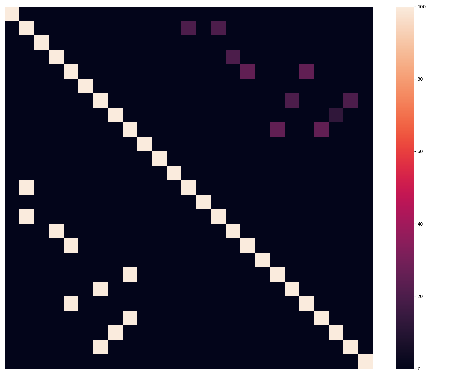
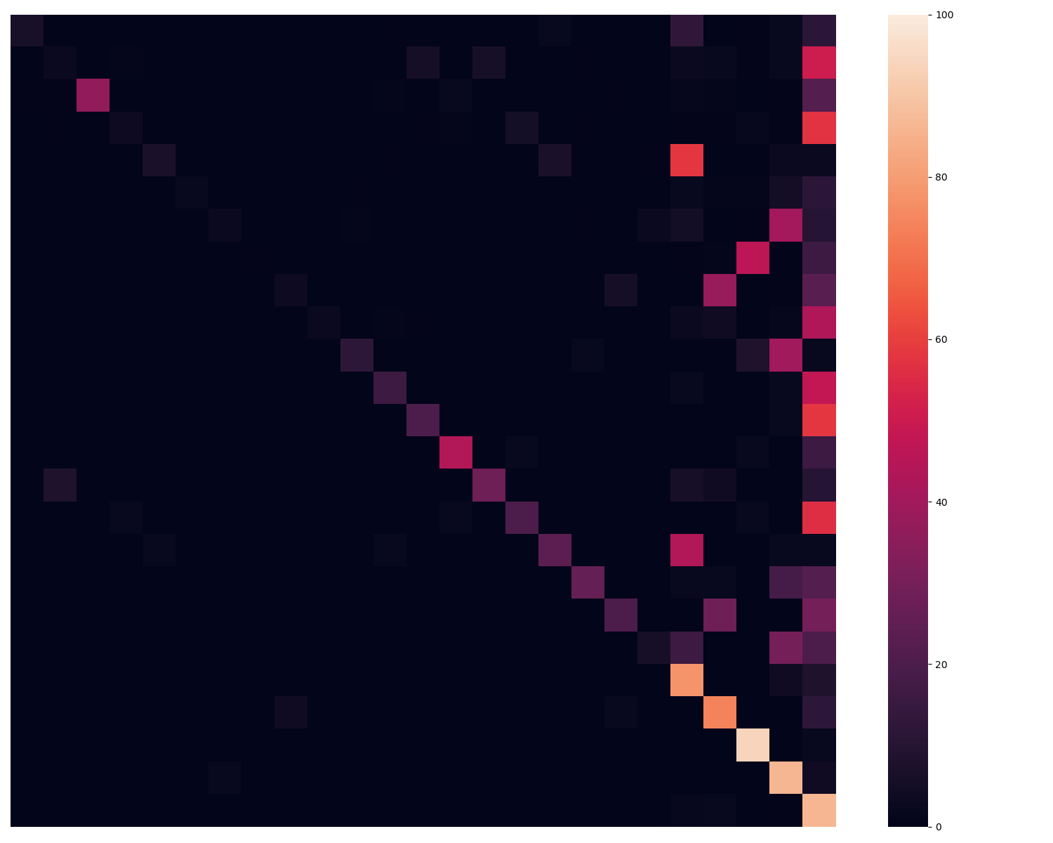
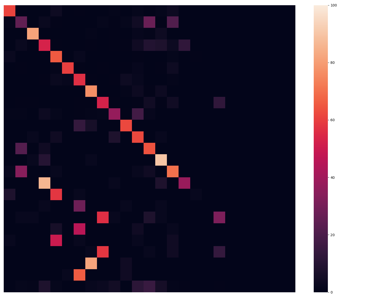
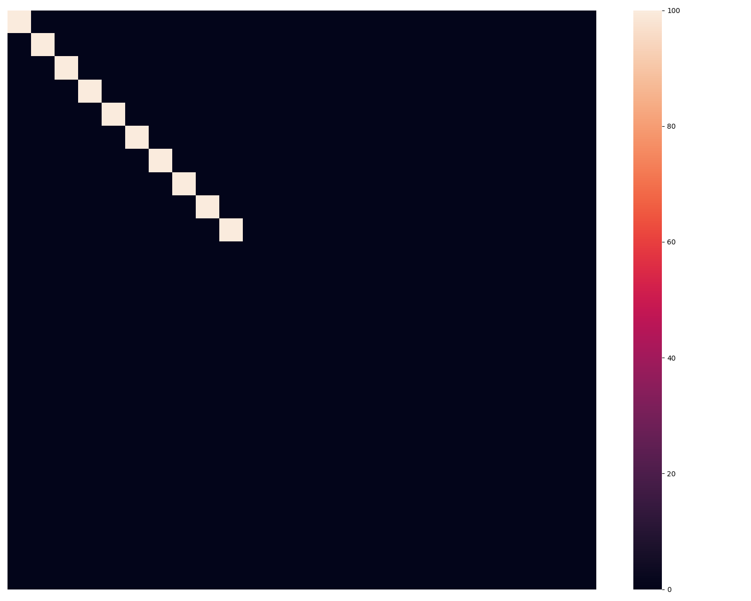
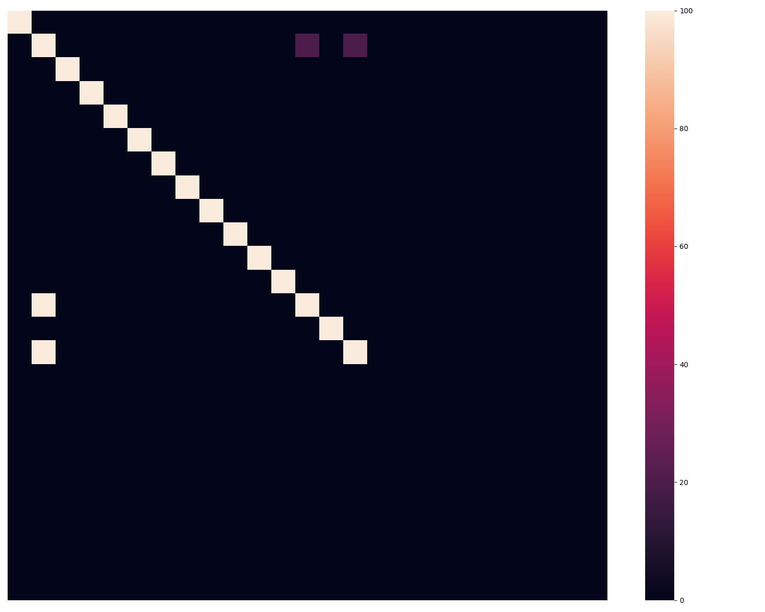
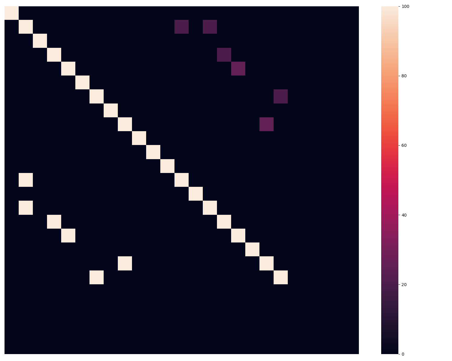
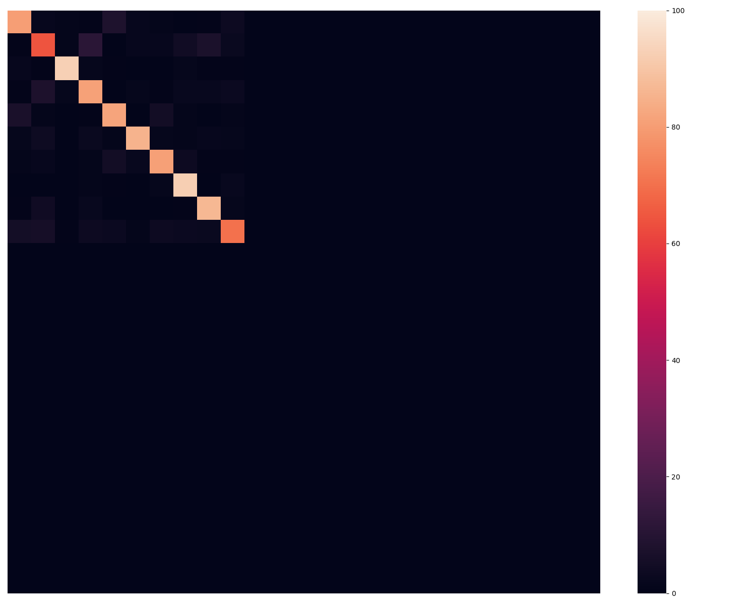
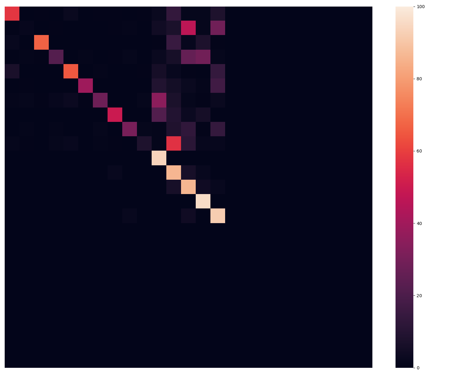
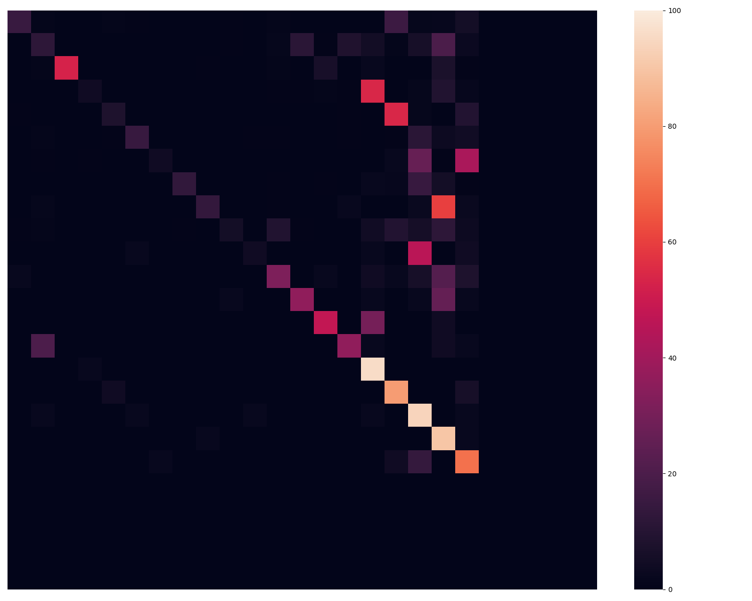
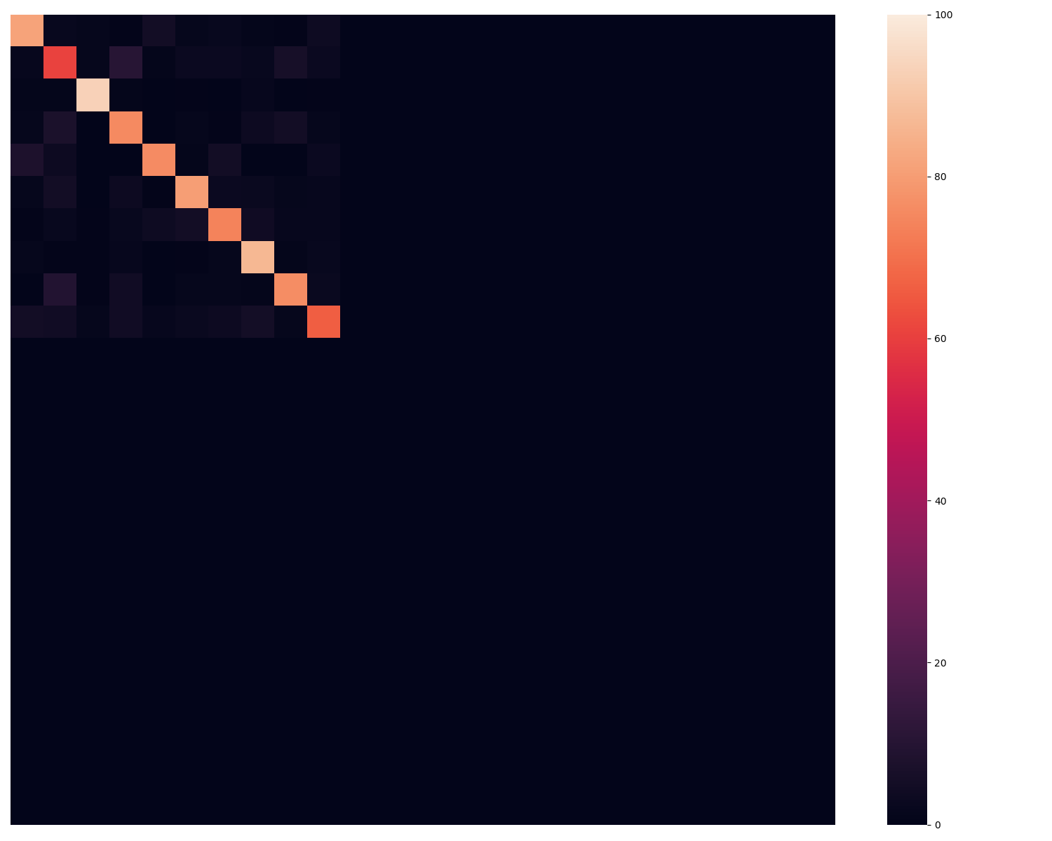
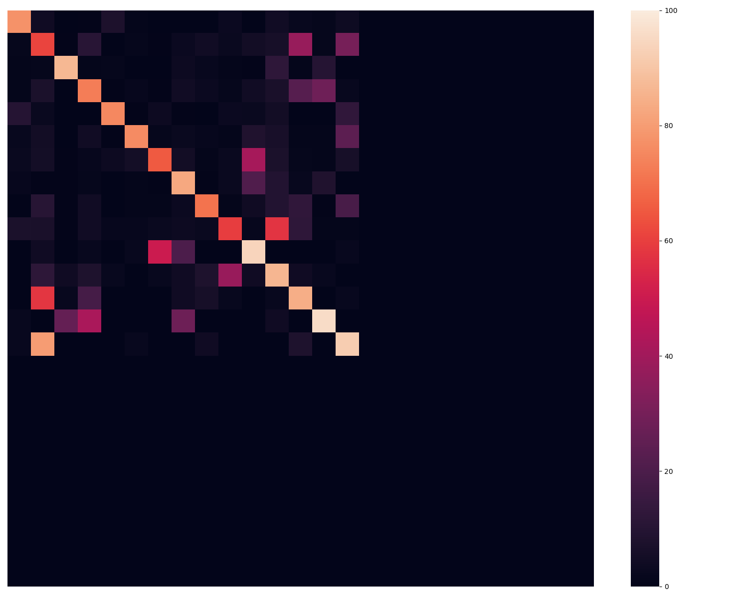
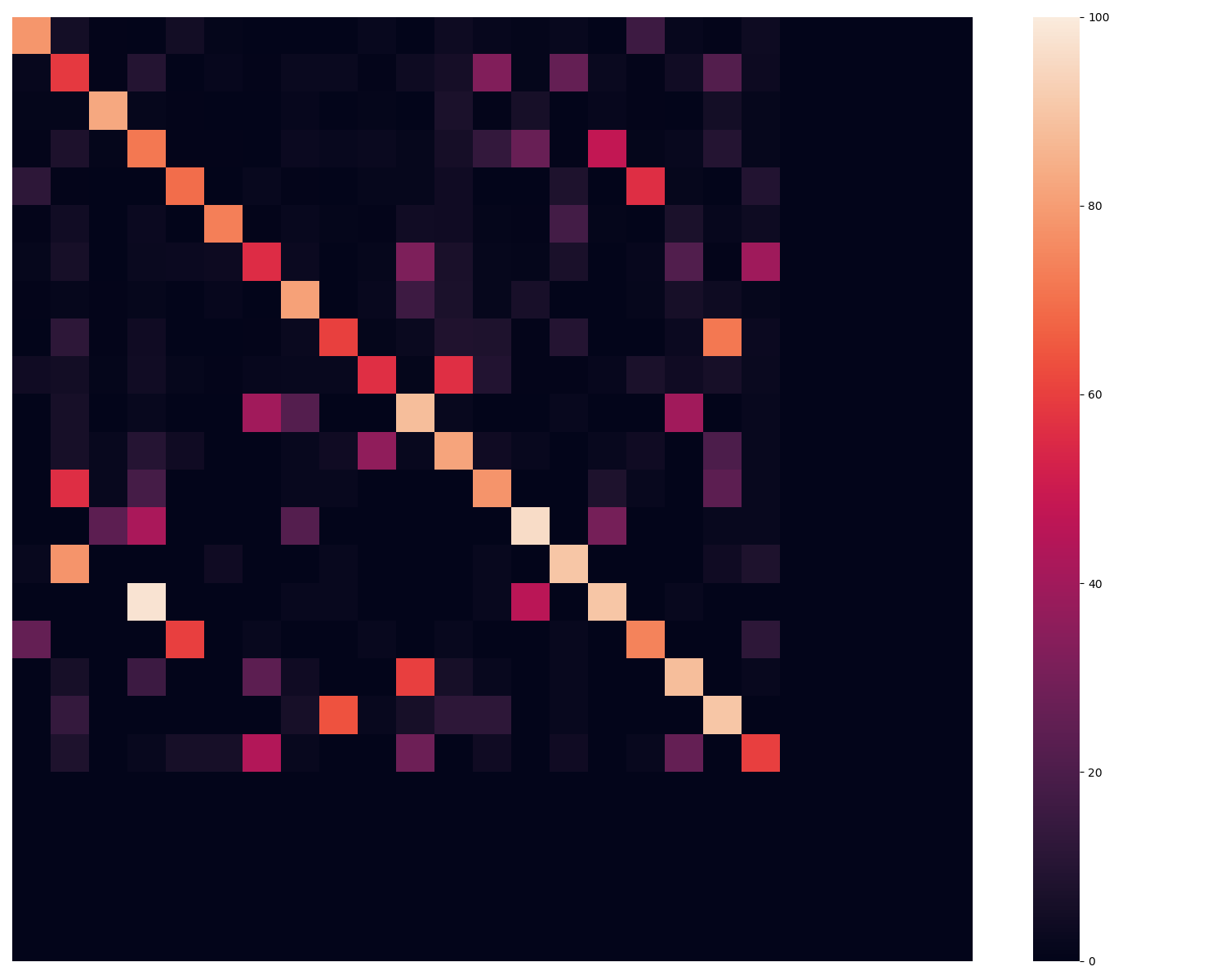
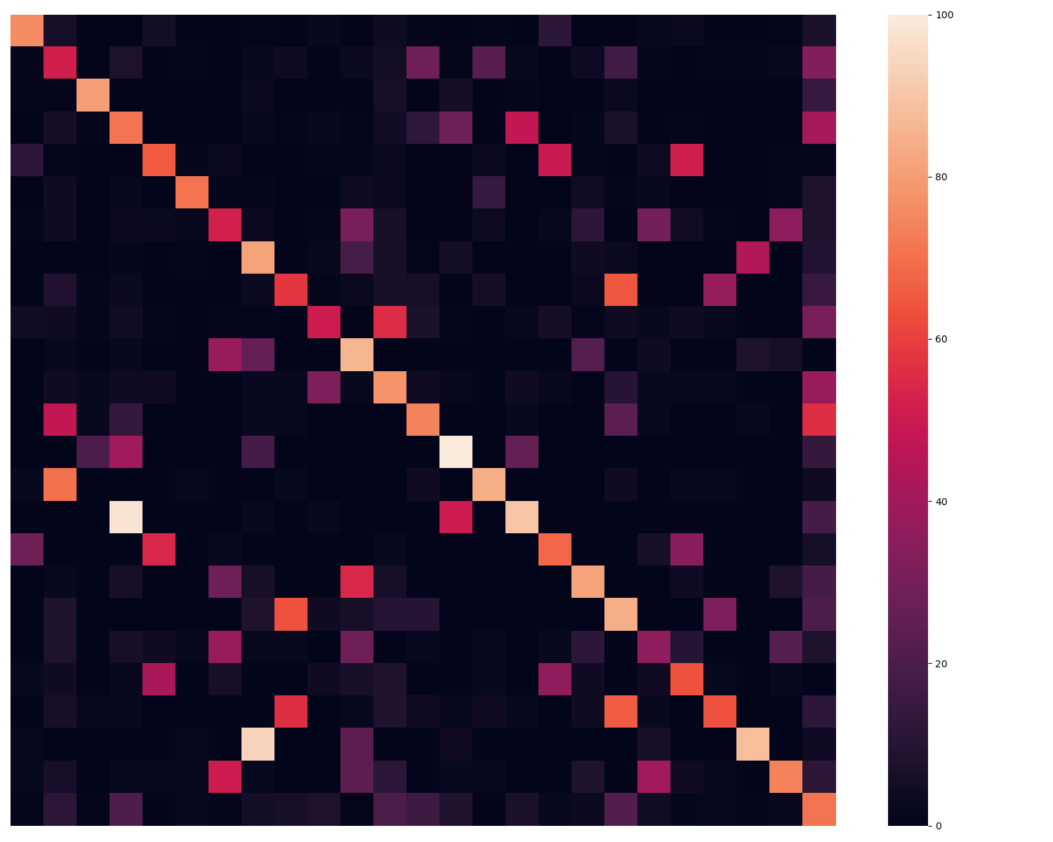
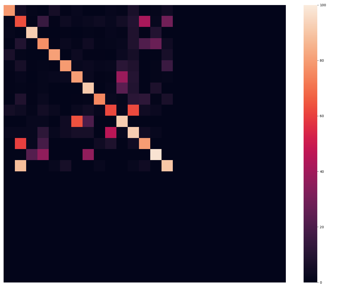
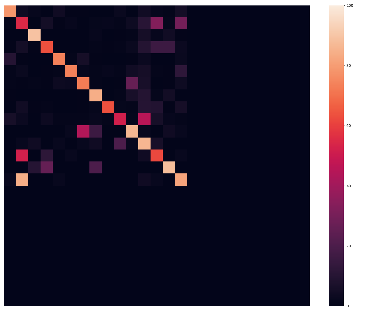
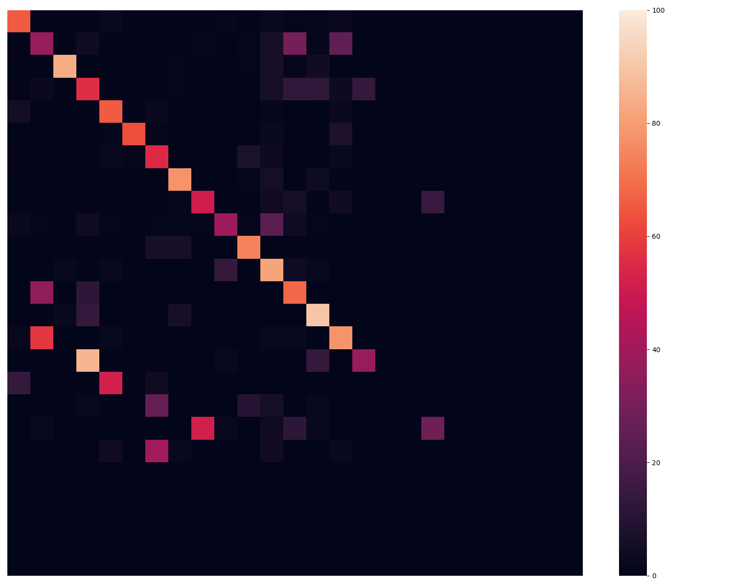
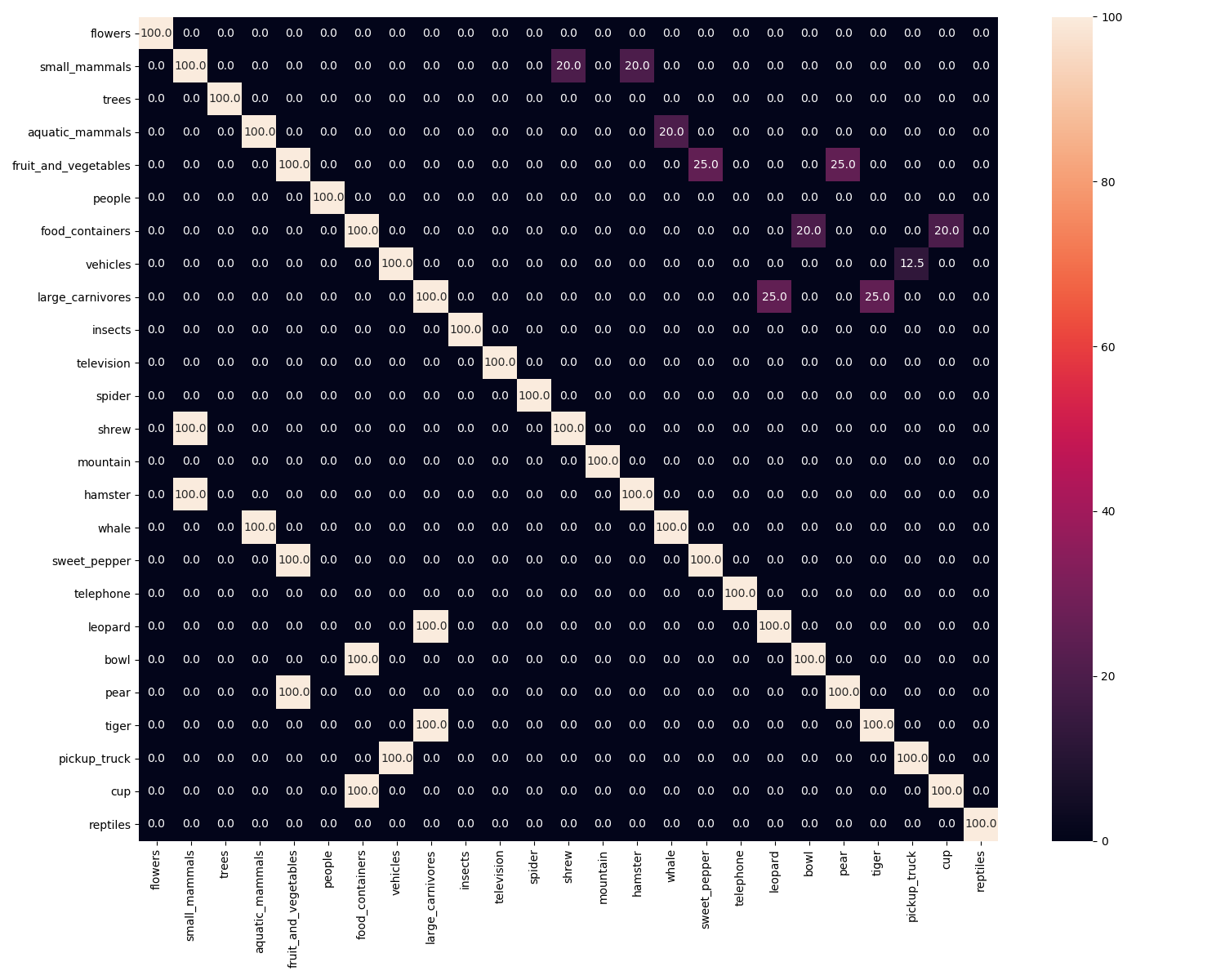
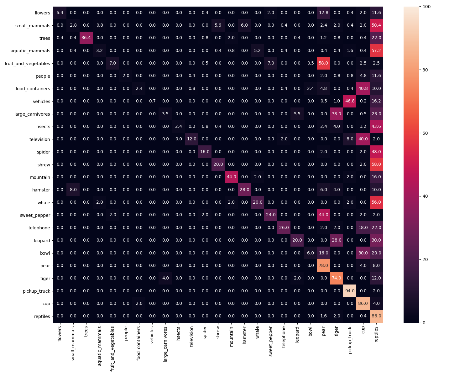
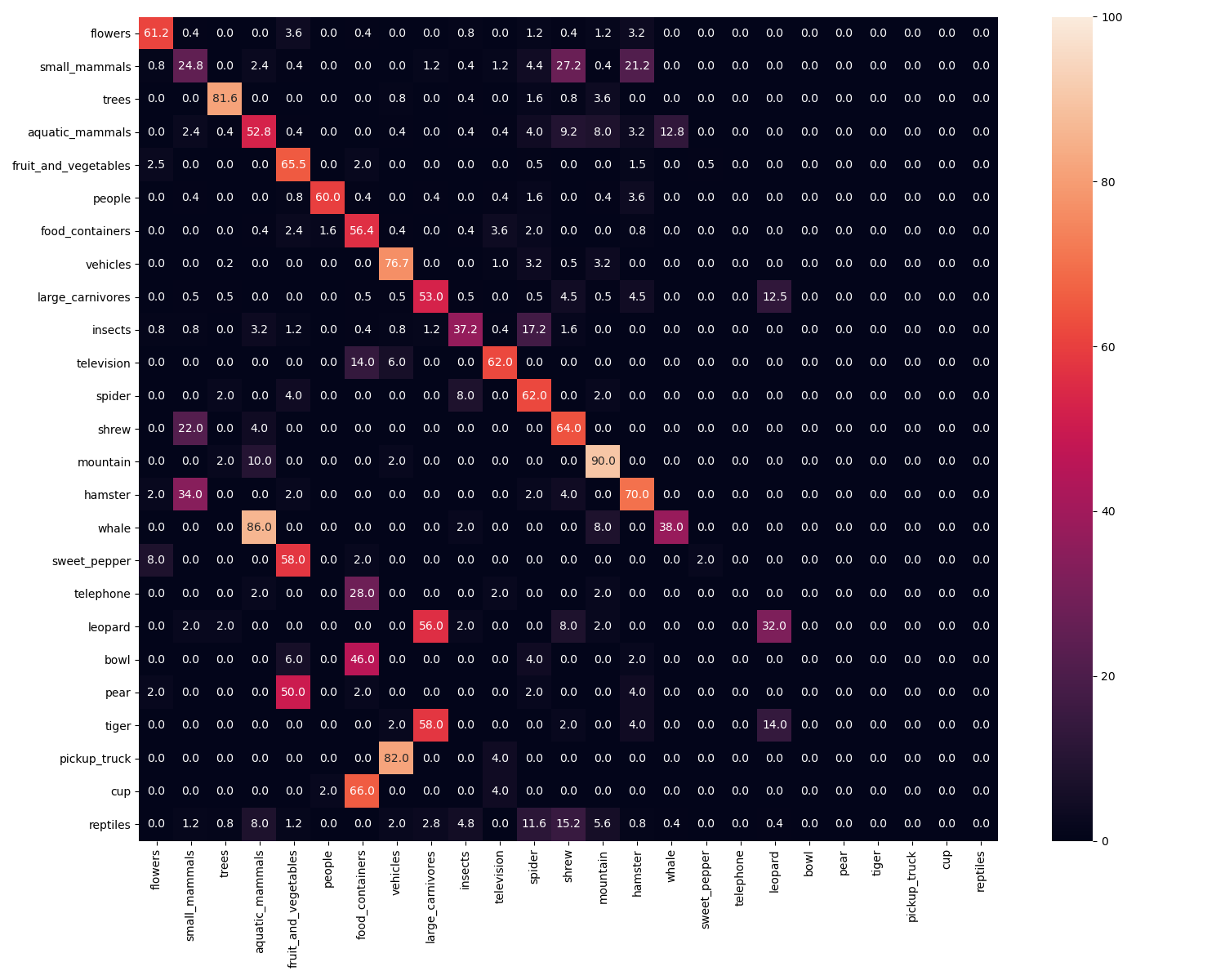
Some other important questions are whether the model correctly associates the newly learned subclass labels to their previously learned superclass, and whether it incorrectly associates the newly learned subclass label with other previously learned subclasses (that have the same superclass). We dig deeper into the confusion matrix (Figure 7) for the predictions of the different models after training on ten tasks of IIRC-CIFAR. Note that in Figure 7, the lower triangular matrix shows the percentage the model predicts older labels for the newly introduced classes, while the upper triangular matrix represents the percentage the model predict newer labels to older classes, with the ground truth being Figure 7(a). The ER method predictions always lie within the newly learned labels (last five classes), as shown in Figure 7(b)) The iCaRL-norm model, as shown in Figure 7(c), performs relatively well in terms of associating (previosuly learned) superclasses to (newly learned) subclasses. For example, whales are always correctly labeled as aquatic mammals, and pickup trucks are correctly labeled as vehicles 94% of the time. However, these models learn some spurious associations as well. For instance, “television” is often mislabeled as “food containers”. Similarly, the model in general correctly associates newer subclasses with older superclasses, but many times it incorrectly associates the subclasses (eg associating “ aquatic mammals” with “whales” 48% of the time and “vehicles” with “pickup trucks” 44% of the time, while by looking at figure 7(a), we see that they only represent 20% and 12.5% of their superclasses respectively) The LUCIR model provides accurate superclass labels to the subclasses. This is shown in Figure 7(d) where LUCIR follows the trends of the ground truth more closely than iCaRL-norm in the lower trianglular part of the confusion matrix. However, it fails to learn new associations. We provide more instances of such plots in the Appendix D.1, which shows that the observed trends are quite general. The full resolution figures for Figure 7 are provided in Appendix D.2.

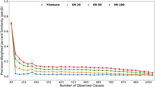
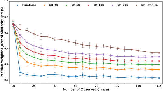
Finally, we provide some ablations for the effect of the buffer size using ER in Appendix E. We can see that using ER even with a buffer size of 100 samples per class gives very poor performance in the case of IIRC-ImageNet, and hence a smarter strategy is needed for this setup.

7 Conclusion

We introduced the “Incremental Implicitly-Refined Classification (IIRC)” setup, a novel extension for the class incremental learning setup where incoming batches of classes have labels at different granularity. Our setup enables studying different challenges in the lifelong learning setup that are difficult to study in the existing setups. Moreover, we proposed a standardized benchmark for evaluating the different models on the IIRC setup. We analyze the performance of several well-known lifelong learning models to give a frame of reference for future works and to bring out the strengths and limitations of different approaches. We hope this work will provide a useful benchmark for the community to focus on some important but under-studied problems in lifelong learning.

Appendix

Appendix A Models Hyperparameter Details

We use SGD as optimizer, as it performs better in the continual learning setups [34], with a momentum value of $0.9$. For the IIRC-CIFAR experiments, The learning rate starts with $1.0$ and is decayed by a factor of $10$ on plateau of the performance of the peri-task validation subset that corresponds to the current task. For the IIRC-ImageNet experiments, the learning rate starts with $0.5$ in the case of iCaRL-CNN and iCaRL-norm, and $0.1$ in the case of finetune, ER and LUCIR, and is decayed by a factor of $10$ on plateau. The number of training epochs per task is $140$ for IIRC-CIFAR and $100$ for IIRC-ImageNet, with the first task always trained for double the number of epochs (due to its larger size). We set the batch size to $128$ and the weight decay parameter to $1e-5$. Moreover, We set the A-GEM memory batch size, which is used to calculate the reference gradient, to $128$. For LUCIR, the margin threshold $m$ is set to $0.5$, and $\lambda_{\text{base}}$ is set to 5. All the hyperparameters were tuned based on the validation performance in experiments that include only the first four tasks.

During training, data augmentations are applied as follows: for IIRC-ImageNet, a random crop of size ($224\times 224$) is sampled from an image, a random horizontal flip is applied, then the pixels are normalized by a pre-calculated per-channel mean and standard deviation. In IIRC-CIFAR, a padding of size $4$ is added to each size, then a random crop of size ($32\times 32$) is sampled, a random horizontal flip is applied, then the pixels are normalized.

We keep a fixed number of samples per class in the replay buffer (20, except otherwise indicated). Hence, the capacity increases linearly as the model learns more classes. These samples are chosen randomly, except for iCaRL and LUCIR which use the herding approach. IIRC-CIFAR experiments are averaged over ten task configurations and the each version of IIRC-ImageNet is averaged over $5$ task configurations (see 4 for details).

Appendix B Baselines Details

Following are three well known baselines that we used to evaluate in the IIRC setup along other baselines including finetune, joint and incremental joint, Vanilla Experience Re-play (ER), and Experience Replay with infinite buffer (ER-infinite).

iCaRL:

iCaRL [38] was among the first deep learning methods to use exemplar rehearsal in order to alleviate the catastrophic forgetting in the class incremental learning setup. iCaRL model updates the model parameters using the distillation loss, where the outputs of the previous network are used as soft labels for the current network. Moreover, it uses the nearest-mean-of-exemplars classifications (NMC) strategy to classify test samples during inference. Since it is difficult to use NMC when the number of labels is variable (not a single label setup), we use the classification layer used during training during inference as well.

Unified learning via rebalancing (LUCIR):

LUCIR [20] is a class incremental method that exploits three components to alleviate the catastrophic forgetting and reduce the negative effect of the imbalance between the old and new classes, since the number of samples in the replay buffer is much less than the current task samples. LUCIR uses the cosine normalization to get balanced magnitudes for classes seen so far. It also uses the less forget constraint, where the distillation loss is applied in the feature space instead of the output space, and a margin ranking loss to ensure interclass separation.

A-GEM:

A-GEM [9] is an improved version of GEM that is a constrained optimization method in the Replay-based approach. GEM uses memory to constrain gradients so as to update the model parameters to not interfere with previous tasks. GEM is a very computationally expensive approach that is not applicable to the large-scale setup. Hence, Averaged GEM (A-GEM) provides an efficient version of GEM, where it only requires computing the gradient on a random subset of memory examples, and it does not need as well to solve any quadratic program but just an inner product. Since A-GEM is a very well known constrained optimization method that has reasonable guarantees in terms of average accuracy in comparison to GEM, we selected it as a candidate to evaluate its performance in our more realistic large scale setting.

Appendix C IIRC Dataset Statistics

	with duplicates		without duplicates
dataset	train	in-task validation	train	in-task validation	post-task validation	test
IIRC-CIFAR	46,160	5,770	40,000	5,000	5,000	10,000
IIRC-Imagenet-full	1,215,123	51,873	1,131,966	48,802	51,095	49,900

Table 1: The number of samples for each split of the training set. with duplicates represents the number of samples including the dublicates between some superclasses and their subclasses (the samples that the model see two times with two different labels). This doesn’t happen for the post-task validation set and test set as they are in the complete information setup

dataset	superclasses	subclasses (under superclasses)	subclasses (with no superclasses)	total
IIRC-CIFAR	15	77	23	115
IIRC-Imagenet-full	85	788	210	1083

Table 2: For each dataset, these are the number of superclasses, the number of subclasses that belong to these superclasses, the number of subclasses that don’t have a superclass, and the total number of superclasses and subclasses

dataset	superclass	num of subclasses	superclass size	subclass	subclass size
IIRC-CIFAR	vehicles	8	1,280	bus	320
IIRC-CIFAR	small mammals	5	800	squirrel	320
IIRC-CIFAR	-	-	-	mushroom	400
IIRC-ImageNet	bird	58	3,762	ostrich	956
IIRC-ImageNet	big cat	6	2,868	leopard	956
IIRC-ImageNet	keyboard instrument	4	1,912	grand piano	956
IIRC-ImageNet	-	-	-	wooden spoon	1,196

Table 3: Several examples for classes and the number of samples they have in the training set. The subclass on the right is a subclass that belongs to the superclass on the left. The left side is blank for subclasses that have no superclasses.

Appendix D More Figures

Figure A.8: Average performance on IIRC-CIFAR. (left) the precision-weighted Jaccard Similarity and (right) the Jaccard Similarity. We run experiments ten times using ten different task configurations to report the performance with the mean and the standard deviation.

(a) Task 0

(b) Task 5

(c) Task 10

(d) Task 15

Figure A.9: IIRC-ImageNet-full Performance on four middle tasks throughout the whole training process, to measure their catastrophic forgetting and backward transfer. Note that a degradation in performance is not necessarily caused by catastrophic forgetting, as a new subclass of a previously observed superclass might be introduced and the model would be penalized for not applying that label retroactively. We run experiments on ten different task configurations and report the performance with the mean and the standard deviation.

(a) Task 0

(b) Task 5

(c) Task 10

(d) Task 15

Figure A.10: IIRC-CIFAR Performance on four middle tasks throughout the whole training process, to measure their catastrophic forgetting and backward transfer. Note that a degradation in performance is not necessarily caused by catastrophic forgetting, as a new subclass of a previously observed superclass might be introduced and the model would be penalized for not applying that label retroactively. We run experiments on ten different task configurations and report the performance with the mean and the standard deviation.

D.1 Confusion Matrix Over time

(a) After task 0

(b) After task 1

(c) After task 5

(d) After task 10

Figure A.11: Ground Truth confusion matrix after introducing tasks 0, 1, 5, 10 of IIRC-CIFAR respectively. The y-axis is the correct label (or one of the correct labels). The x-axis is the model predicted labels. Labels are arranged by their order of introduction. Only 25 labels are shown for better visibility.

(a) After task 0

(b) After task 1

(c) After task 5

(d) After task 10

Figure A.12: ER confusion matrix after introducing tasks 0, 1, 5, 10 of IIRC-CIFAR respectively. The y-axis is the correct label (or one of the correct labels). The x-axis is the model predicted labels. Labels are arranged by their order of introduction. Only 25 labels are shown for better visibility.

(a) After task 0

(b) After task 1

(c) After task 5

(d) After task 10

Figure A.13: iCaRL-CNN confusion matrix after introducing tasks 0, 1, 5, 10 of IIRC-CIFAR respectively. The y-axis is the correct label (or one of the correct labels). The x-axis is the model predicted labels. Labels are arranged by their order of introduction. Only 25 labels are shown for better visibility.

(a) After task 0

(b) After task 1

(c) After task 5

(d) After task 10

Figure A.14: iCaRL-norm confusion matrix after introducing tasks 0, 1, 5, 10 of IIRC-CIFAR respectively. The y-axis is the correct label (or one of the correct labels). The x-axis is the model predicted labels. Labels are arranged by their order of introduction. Only 25 labels are shown for better visibility.

(a) After task 0

(b) After task 1

(c) After task 5

(d) After task 10

Figure A.15: LUCIR confusion matrix after introducing tasks 0, 1, 5, 10 of IIRC-CIFAR respectively. The y-axis is the correct label (or one of the correct labels). The x-axis is the model predicted labels. Labels are arranged by their order of introduction. Only 25 labels are shown for better visibility.

D.2 Full Resolution Confusion Matrix

Figure A.16: Confusion matrix (ground truth) after training on task 10 of IIRC-CIFAR. the y-axis is the correct label (or one of the correct labels), the x-axis is the model predicted labels, The classes are arranged by their order of introduction. Only 25 classes are shown for better visibility. The y-axis represents the true label (or one of the true labels), while the x-axis represents the model predictions.

Figure A.17: Confusion matrix (ER) after training on task 10 of IIRC-CIFAR. the y-axis is the correct label (or one of the correct labels), the x-axis is the model predicted labels, The classes are arranged by their order of introduction. Only 25 classes are shown for better visibility. The y-axis represents the true label (or one of the true labels), while the x-axis represents the model predictions.

Figure A.18: Confusion matrix (iCaRL-norm) after training on task 10 of IIRC-CIFAR. The x-axis is the model predicted labels, The classes are arranged by their order of introduction. Only 25 classes are shown for better visibility. The y-axis represents the true label (or one of the true labels), while the x-axis represents the model predictions.

Figure A.19: Confusion matrix (LUCIR) after training on task 10 of IIRC-CIFAR. The x-axis is the model predicted labels, The classes are arranged by their order of introduction. Only 25 classes are shown for better visibility. The y-axis represents the true label (or one of the true labels), while the x-axis represents the model predictions.

Appendix E Effect of Buffer

Figure A.20: Imagenet average performance using different buffer sizes, The number next to ER indicates the number of samples per class used for the replay buffer

Figure A.21: CIFAR average performance using different buffer sizes, The number next to ER indicates the number of samples per class used for the replay buffer

Appendix F Pseudo Codes

Require : $tasks$  // A list of the classes to-be-introduced at each task

$trainSet,\;validSet_{inTask},\;validSet_{postTask},\;testSet$ $\leftarrow$ LoadDatasets()

$model$ $\leftarrow$ CreateModel()

/* create an empty buffer */

$buffer$ $\leftarrow$ CreateBuffer()

for $task$ in $tasks$ do

       $model$ $\leftarrow$ TrainOnTask($model,\;buffer,\;trainingSet,\;validSet_{inTask}$)

       /* add randomly selected samples to buffer */

       $buffer$ $\leftarrow$ AddToBuffer ($buffer,\;trainingSet$)

       PostTaskEvaluate($model,\;validSet_{postTask},\;testSet$)

      

end for

Algorithm 1 IncrementalTrain

input : $rawData_{train}$   // The default single-label full dataset (train)

input : $rawData_{test}$  // The default single-label full dataset (test)

input : $classHierarchy$  // A dictionary that maps each superclass to its constituent subclasses

$multilabeledData_{train}$ $\leftarrow$ AddSuperclassLabels($rawData_{train},\;classHierarchy$)

$multilabeledData_{test}$ $\leftarrow$ AddSuperclassLabels($rawData_{test},\;classHierarchy$)

$multilabeledData_{train},\;multilabeledData_{valid_{inTask}},\;multilabeledData_{valid_{postTask}}$ $\leftarrow$ SplitData($multilabeledData_{train}$)

$trainSet$ $\leftarrow$ IncompleteInfoIncrementalDataset($multilabeledData_{train}$)

$validSet_{inTask}$ $\leftarrow$ IncompleteInfoIncrementalDataset($multilabeledData_{valid_{inTask}}$)

$validSet_{postTask}$ $\leftarrow$ CompleteInfoIncrementalTestDataset($multilabeledData_{valid_{postTask}}$)

$testSet$ $\leftarrow$ CompleteInfoIncrementalTestDataset($multilabeledData_{test}$)

output : $trainSet$  // The incomplete information incremental learning training set

output : $validSet_{inTask}$  // The incomplete information incremental learning validation set (for in-task performance)

output : $validSet_{postTask}$  // The complete information incremental learning validation set (for post-task performance)

output : $testSet$  // The complete information incremental learning test set

Algorithm 2 LoadDatasets

input : $multilabelData$  // A list of samples with each sample in the form of ($image$, ($superclassLabel,\;subclassLabel$)) or ($image$, ($subclassLabel$)))

input : $superclassToSubclass$  // a mapping that maps superclasses to their constituent subclasses

input : $tasks$  // The classes to-be-introduced at each task

Require : $subclasses$  // All refined subclasses (those who have a superclass as well as those who don’t)

output : a dataset object with the data changing along the tasks

Initialization:

$classToDataIndices$ $\leftarrow$ EmptyDictionary

$currentTaskId$ $\leftarrow$ 0

$dataIndices_{task}$ $\leftarrow$ []

for $subclass$ in $subclasses$ do

       /* get the indices of the samples which correspond to this subclass */

       $dataIndices_{subclass}$ $\leftarrow$ GetSamplesIndices($mtultilabelData,\;subclass$)

       if $subclass$ has superclass then

             $dataSubsetLength_{superclass}$ $\leftarrow$ 0.4 * Length($dataIndices_{subclass}$)

             $dataSubsetLength_{subclass}$ $\leftarrow$ 0.8 * Length($dataIndices_{subclass}$)

             $dataIndices_{subclass}$ $\leftarrow$ Shuffle($dataIndices_{subclass}$)

             $dataSubsetIndices_{subclass}$ $\leftarrow$ $dataIndices_{subclass}$[:$dataSubsetLength_{subclass}$]

             $dataSubsetIndices_{superclass}$ $\leftarrow$ $dataIndices_{subclass}$[-$dataSubsetLength_{superclass}$:]

             $classToDataIndices$[$subclass$] $\leftarrow$ $dataIndices_{subclass}$

             $classToDataIndices$[$superclass$] $\leftarrow$ $classToDataIndices$[$superclass$] $\cup$ $dataSubsetIndices_{superclass}$

            

       end if

      else if $subclass$ has no superclass then

             $classToDataIndices$[subclass] $\leftarrow$ $dataIndices_{subclass}$

            

       end if

      

end for

IncrementTask:

$currentTaskId$ $\leftarrow$ $currentTaskId+1$

$dataIndices_{task}$ $\leftarrow$ []

for $class$ in $tasks$[$currentTaskId$] do

       $dataIndices_{task}$ $\leftarrow$ $dataIndices_{task}$ $\cup$ $classToDataIndices$[$class$]

      

end for

GetItem:

Require : $classes_{task}$  // The classes present in the current task

input : $index$  // an index in the range of length of $dataIndices_{task}$

$image,\;labels$ $\leftarrow$ $multilabelData$[$dataIndices_{task}$[$index$]]

$label$ $\leftarrow$ $labels\cap classes_{task}$

output : $image$  // The sample image

output : $label$  // The label corresponding to this image that exists in the current task

Algorithm 3 IncompleteInfoIncrementalDataset

input : $multilabelData$  // A list of samples with each sample in the form of ($image$, ($superclassLabel,\;subclassLabel$)) or ($image$, ($subclassLabel$)))

input : $superclassToSubclass$  // a mapping that maps superclasses to their constituent subclasses

input : $tasks$  // The classes available at each task

Require : $subclasses$  // All refined subclasses (those who have a superclass as well as those who don’t)

output : a test dataset object which keeps collecting data along the tasks

Initialization:

$classToDataIndices$ $\leftarrow$ empty_dictionary

$classes_{observed}$ $\leftarrow$ []

$dataIndices_{accessible}\leftarrow$ []

for $subclass$ in $subclasses$ do

       /* get the indices of the samples which correspond to this subclass */

       $dataIndices_{subclass}$ $\leftarrow$ GetSamplesIndices($multilabelData,\;subclass$)

       $classToDataIndices$[$subclass$] $\leftarrow$ $dataIndices_{subclass}$

       if subclass has superclass then

             $classToDataIndices$[$superclass$] $\leftarrow$ $classToDataIndices$[$superclass$] $\cup$ $classToDataIndices$[$subclass$]

            

       end if

      

end for

LoadTask

input : $taskId$  // The index of the task to load

$dataIndices_{accessible}$ $\leftarrow$ []

$classes_{observed}$ $\leftarrow$ $classes_{observed}$ $\cup$ $tasks$[$taskId$]

for $class$ in $tasks$[$taskId$] do

       $dataIndices_{accessible}$ $\leftarrow$ $dataIndices_{accessible}\cup classToDataIndices$[$class$]

end for

LoadAllObservedData

Require : $classes_{observed}$  // All classes observed till now in all previous tasks

$dataIndices_{accessible}$ $\leftarrow$ []

for $class$ in $classes_{observed}$ do

       $dataIndices_{accessible}\leftarrow dataIndices_{accessible}\cup classToDataIndices$[$class$]

end for

$dataIndices_{accessible}\leftarrow$ RemoveDuplicates($dataIndices_{accessible})$

GetItem

Require : $classes_{observed}$  // All classes observed till now in all previous tasks

input : $index$  // an index in the range of task_data_indices

$image,\;labels$ $\leftarrow$ $multilabelData$[$dataIndices_{accessible}$[$index$]]

$labels$ $\leftarrow$ $labels$ $\cap$ $classes_{observed}$

output : $image$  // The sample image

output : $labels$  // The labels corresponding to this image that exist in the $classes_{observed}$

Algorithm 4 CompleteInfoIncrementalTestDataset

Appendix G IIRC Datasets Hierarchies

G.1 IIRC-CIFAR Hierarchy

superclass	subclasses
aquatic mammals	beaver, dolphin, otter, seal, whale
fish	aquarium fish, flatfish, ray, shark, trout
flowers	orchid, poppy, rose, sunflower, tulip
food containers	bottle, bowl, can, cup, plate
fruit and vegetables	apple, orange, pear, sweet pepper
household furniture	bed, chair, couch, table, wardrobe
insects	bee, beetle, butterfly, caterpillar, cockroach
large carnivores	leopard, lion, tiger, wolf
large omnivores and herbivores	bear, camel, cattle, chimpanzee, elephant, kangaroo
medium sized mammals	fox, porcupine, possum, raccoon, skunk
people	baby, boy, girl, man, woman
reptiles	crocodile, dinosaur, lizard, snake, turtle
small mammals	hamster, mouse, rabbit, shrew, squirrel
trees	maple tree, oak tree, palm tree, pine tree, willow tree
vehicles	bicycle, bus, motorcycle, pickup truck, train, streetcar, tank, tractor
-	mushroom, clock, keyboard, lamp, telephone, television, bridge, castle, house, road, skyscraper, cloud, forest, mountain, plain, sea, crab, lobster, snail, spider, worm, lawn mower, rocket

G.2 IIRC-ImageNet Hierarchy

superclass	subclasses
dog	dalmatian, basenji, pug, Leonberg, Newfoundland, Great Pyrenees, Mexican hairless, Brabancon griffon, Pembroke, Cardigan, Chihuahua, Japanese spaniel, Maltese dog, Pekinese, Shih-Tzu, toy terrier, papillon, Blenheim spaniel, Rhodesian ridgeback, boxer, bull mastiff, Great Dane, Saint Bernard, Eskimo dog, Tibetan mastiff, French bulldog, malamute, Siberian husky, Samoyed, Pomeranian, chow, keeshond, toy poodle, miniature poodle, standard poodle, Afghan hound, basset, beagle, bloodhound, bluetick, redbone, Ibizan hound, Norwegian elkhound, otterhound, Saluki, Scottish deerhound, Weimaraner, black-and-tan coonhound, Walker hound, English foxhound, borzoi, Irish wolfhound, Italian greyhound, whippet, Bedlington terrier, Border terrier, Kerry blue terrier, Irish terrier, Norfolk terrier, Norwich terrier, Yorkshire terrier, Airedale, cairn, Australian terrier, Dandie Dinmont, Boston bull, Scotch terrier, Tibetan terrier, silky terrier, soft-coated wheaten terrier, West Highland white terrier, Lhasa, Staffordshire bullterrier, American Staffordshire terrier, wire-haired fox terrier, Lakeland terrier, Sealyham terrier, German short-haired pointer, vizsla, kuvasz, schipperke, Doberman, miniature pinscher, affenpinscher, Brittany spaniel, clumber, cocker spaniel, Sussex spaniel, English springer, Welsh springer spaniel, Irish water spaniel, English setter, Irish setter, Gordon setter, flat-coated retriever, curly-coated retriever, golden retriever, Labrador retriever, Chesapeake Bay retriever, miniature schnauzer, giant schnauzer, standard schnauzer, Greater Swiss Mountain dog, Bernese mountain dog, Appenzeller, EntleBucher, briard, kelpie, komondor, Old English sheepdog, Shetland sheepdog, collie, Border collie, Bouvier des Flandres, Rottweiler, German shepherd, groenendael, malinois
bird	cock, hen, ostrich, bee eater, hornbill, hummingbird, jacamar, toucan, coucal, quail, partridge, peacock, black grouse, ptarmigan, ruffed grouse, prairie chicken, water ouzel, robin, bulbul, jay, magpie, chickadee, brambling, goldfinch, house finch, junco, indigo bunting, black swan, European gallinule, goose, drake, red-breasted merganser, pelican, albatross, king penguin, spoonbill, flamingo, limpkin, bustard, white stork, black stork, American coot, oystercatcher, red-backed sandpiper, redshank, dowitcher, ruddy turnstone, little blue heron, bittern, American egret, African grey, macaw, sulphur-crested cockatoo, lorikeet, vulture, kite, bald eagle, great grey owl
garment	suit, abaya, kimono, cardigan, feather boa, stole, jersey, sweatshirt, poncho, brassiere, jean, gown, military uniform, pajama, apron, academic gown, vestment, bow tie, Windsor tie, fur coat, lab coat, trench coat, hoopskirt, miniskirt, overskirt, sarong, cloak
beverage	espresso, red wine, cup, eggnog
aircraft	airship, balloon, airliner, warplane, wing, space shuttle
bear	brown bear, American black bear, ice bear, sloth bear
fox	red fox, kit fox, Arctic fox, grey fox
wolf	timber wolf, white wolf, red wolf, coyote
bag	backpack, mailbag, plastic bag, purse, sleeping bag
footwear	clog, cowboy boot, Loafer, running shoe, sandal
toiletry	hair spray, lotion, perfume, face powder, sunscreen, lipstick
box	carton, chest, crate, mailbox, pencil box, safe
rodent	hamster, porcupine, marmot, beaver, guinea pig, fox squirrel
bottle	beer bottle, pill bottle, pop bottle, water bottle, wine bottle, water jug, whiskey jug
fabric	velvet, wool, bib, dishrag, handkerchief, bath towel, paper towel
cup	beer glass, goblet, cocktail shaker, measuring cup, pitcher, beaker, coffee mug
fungus	coral fungus, gyromitra, stinkhorn, earthstar, hen-of-the-woods, bolete, agaric
musteline	weasel, mink, polecat, black-footed ferret, otter, skunk, badger
truck	fire engine, garbage truck, pickup, tow truck, trailer truck, moving van, police van, recreational vehicle, forklift, harvester, snowplow, tractor
headdress	crash helmet, football helmet, bearskin, bonnet, cowboy hat, sombrero, bathing cap, mortarboard, shower cap, pickelhaube
ball	baseball, basketball, croquet ball, golf ball, ping-pong ball, punching bag, rugby ball, soccer ball, tennis ball, volleyball
car	ambulance, beach wagon, cab, convertible, jeep, limousine, Model T, racer, sports car, minivan, grille, golfcart
measuring instrument	barometer, scale, odometer, rule, sundial, digital watch, hourglass, parking meter, stopwatch, analog clock, digital clock, wall clock
tool	hammer, plunger, screwdriver, shovel, cleaver, letter opener, can opener, corkscrew, hatchet, chain saw, plane, scabbard, power drill, carpenter’s kit
watercraft	schooner, catamaran, trimaran, fireboat, gondola, canoe, yawl, lifeboat, speedboat, pirate, wreck, container ship, liner, aircraft carrier, submarine, amphibian, paddle
dish	Petri dish, mixing bowl, soup bowl, tray
bus	minibus, school bus, trolleybus
cart	horse cart, jinrikisha, oxcart
tracked vehicle	snowmobile, half track, tank
lamp	candle, spotlight, jack-o’-lantern, lampshade, table lamp
optical instrument	binoculars, projector, sunglasses, lens cap, loupe, Polaroid camera, reflex camera
gymnastic apparatus	balance beam, horizontal bar, parallel bars
swine	hog, wild boar, warthog
rabbits	hare, wood rabbit, Angora
echinoderm	starfish, sea urchin, sea cucumber
wild dog	dingo, dhole, African hunting dog
pouched mammal	wombat, wallaby, koala
aquatic mammal	dugong, grey whale, killer whale, sea lion
person	ballplayer, scuba diver, groom
mollusk	chiton, chambered nautilus, conch, snail, slug, sea slug
weapon	bow, projectile, cannon, missile, rifle, revolver, assault rifle, holster
bovid	bison, water buffalo, ram, ox, bighorn, ibex, hartebeest, impala, gazelle
salamander	European fire salamander, common newt, eft, spotted salamander, axolotl
frog	tree frog, tailed frog, bullfrog
big cat	leopard, snow leopard, jaguar, lion, tiger, cheetah
domestic cat	tabby, tiger cat, Persian cat, Siamese cat, Egyptian cat
cooking utensil	spatula, frying pan, wok, Crock Pot, Dutch oven, caldron, coffeepot, teapot
primate	Madagascar cat, indri, gibbon, siamang, orangutan, gorilla, chimpanzee, marmoset, capuchin, howler monkey, titi, spider monkey, squirrel monkey, guenon, patas, baboon, macaque, langur, colobus, proboscis monkey
fish	barracouta, electric ray, stingray, hammerhead, great white shark, tiger shark, sturgeon, gar, puffer, rock beauty, anemone fish, lionfish, eel, tench, goldfish, coho
lizard	banded gecko, common iguana, American chameleon, whiptail, agama, frilled lizard, alligator lizard, Gila monster, green lizard, African chameleon, Komodo dragon
turtle	mud turtle, terrapin, box turtle, loggerhead, leatherback turtle
spider	black and gold garden spider, barn spider, garden spider, black widow, tarantula, wolf spider, spider web
insect	ringlet, sulphur butterfly, lycaenid, cabbage butterfly, monarch, admiral, dragonfly, damselfly, lacewing, cicada, leafhopper, cockroach, mantis, walking stick, grasshopper, cricket, bee, ant, fly, tiger beetle, ladybug, ground beetle, long-horned beetle, leaf beetle, weevil, dung beetle, rhinoceros beetle
green groceries	acorn, hip, ear, fig, pineapple, banana, jackfruit, custard apple, pomegranate, strawberry, orange, lemon, Granny Smith, buckeye, rapeseed, corn, cucumber, artichoke, cardoon, mushroom, bell pepper, mashed potato, zucchini, spaghetti squash, acorn squash, butternut squash, broccoli, cauliflower, head cabbage
keyboard instrument	accordion, organ, grand piano, upright
percussion instrument	chime, drum, gong, maraca, marimba, steel drum
stringed instrument	banjo, acoustic guitar, electric guitar, cello, violin, harp
wind instrument	ocarina, harmonica, flute, panpipe, bassoon, oboe, sax, cornet, French horn, trombone
crustacean	isopod, crayfish, hermit crab, spiny lobster, American lobster, Dungeness crab, rock crab, fiddler crab, king crab
pen	ballpoint, fountain pen, quill
display	desktop computer, laptop, notebook, screen, television, monitor
electronic equipement	cassette player, CD player, modem, oscilloscope, tape player, iPod, printer, joystick, dial telephone, pay-phone, cellular telephone, mouse, hand-held computer
snake	sea snake, horned viper, boa constrictor, rock python, Indian cobra, green mamba, diamondback, sidewinder, thunder snake, ringneck snake, hognose snake, green snake, king snake, garter snake, water snake, vine snake, night snake
geological formation	cliff, geyser, lakeside, seashore, valley, promontory, alp, volcano, coral reef, sandbar
food	dough, guacamole, chocolate sauce, carbonara, French loaf, bagel, pretzel, plate, trifle, ice cream, ice lolly, pizza, potpie, burrito, consomme, hot pot, hotdog, cheeseburger, meat loaf
white home appliances	dishwasher, refrigerator, washer, stove
kitchen appliances	microwave, toaster, waffle iron, espresso maker
wheel	car wheel, paddlewheel, pinwheel, potter’s wheel, reel, disk brake
seat	toilet seat, studio couch, park bench, barber chair, folding chair, rocking chair, throne
baby bed	bassinet, cradle, crib
cabinet	medicine chest, wardrobe, china cabinet, bookcase, chiffonier, file, entertainment center, plate rack
table	desk, pool table, dining table
bridges	steel arch bridge, suspension bridge, viaduct
fence	chainlink fence, picket fence, stone wall, worm fence
long structures	beacon, obelisk, totem pole
movable homes	mountain tent, mobile home, yurt
building	planetarium, barn, cinema, boathouse, palace, monastery, castle, dome, church, mosque, stupa, bell cote, thatch, tile roof, triumphal arch
body armor	chain mail, cuirass, bulletproof vest, breastplate
mask	mask, oxygen mask, gasmask, ski mask
curtain-screen	window shade, shower curtain, theater curtain
bike	moped, bicycle-built-for-two, tricycle, unicycle, mountain bike, motor scooter
train	passenger car, freight car, electric locomotive, bullet train, streetcar, steam locomotive
swimsuit	bikini, maillot, swimming trunks
socks mittens	Christmas stocking, mitten, sock
keyboard	computer keyboard, space bar, typewriter keyboard
-	African crocodile, American alligator, triceratops, trilobite, harvestman, scorpion, tick, centipede, tusker, echidna, platypus, jellyfish, sea anemone, brain coral, flatworm, nematode, crane, hyena, cougar, lynx, mongoose, meerkat, sorrel, zebra, hippopotamus, Arabian camel, llama, armadillo, three-toed sloth, Indian elephant, African elephant, lesser panda, giant panda, abacus, altar, apiary, ashcan, bakery, Band Aid, bannister, barbell, barbershop, barrel, barrow, bathtub, binder, birdhouse, bobsled, bolo tie, bookshop, bottlecap, brass, breakwater, broom, bucket, buckle, butcher shop, car mirror, carousel, cash machine, cassette, chain, cliff dwelling, coil, combination lock, confectionery, crutch, dam, diaper, dock, dogsled, doormat, drilling platform, drumstick, dumbbell, electric fan, envelope, fire screen, flagpole, fountain, four-poster, gas pump, go-kart, greenhouse, grocery store, guillotine, hair slide, hamper, hand blower, hard disc, home theater, honeycomb, hook, iron, jigsaw puzzle, knee pad, knot, ladle, lawn mower, library, lighter, loudspeaker, lumbermill, magnetic compass, manhole cover, matchstick, maypole, maze, megalith, microphone, milk can, mortar, mosquito net, mousetrap, muzzle, nail, neck brace, necklace, nipple, oil filter, packet, padlock, paintbrush, parachute, patio, pedestal, pencil sharpener, photocopier, pick, pier, piggy bank, pillow, plow, pole, pot, prayer rug, prison, puck, quilt, racket, radiator, radio, radio telescope, rain barrel, remote control, restaurant, rotisserie, rubber eraser, safety pin, saltshaker, scoreboard, screw, seat belt, sewing machine, shield, shoe shop, shoji, shopping basket, shopping cart, ski, slide rule, sliding door, slot, snorkel, soap dispenser, solar dish, space heater, spindle, stage, stethoscope, strainer, stretcher, sunglass, swab, swing, switch, syringe, teddy, thimble, thresher, tobacco shop, torch, toyshop, tripod, tub, turnstile, umbrella, vacuum, vase, vault, vending machine, wallet, washbasin, water tower, whistle, wig, window screen, wooden spoon, web site, comic book, crossword puzzle, street sign, traffic light, book jacket, menu, hay, bubble, daisy, yellow lady’s slipper, toilet tissue

Appendix H Results in Tables

task	model
	ER	iCaRL-CNN	iCaRL-norm	LUCIR	AGEM	incremental joint	ER-infinite
0	0.72 (0.039)	0.71 (0.042)	0.75 (0.037)	0.74 (0.036)	0.72 (0.032)	0.71 (0.032)	0.72 (0.033)
1	0.31 (0.046)	0.47 (0.032)	0.5 (0.035)	0.5 (0.101)	0.15 (0.024)	0.7 (0.035)	0.64 (0.067)
2	0.23 (0.054)	0.36 (0.017)	0.39 (0.024)	0.35 (0.178)	0.1 (0.023)	0.67 (0.029)	0.63 (0.029)
3	0.2 (0.027)	0.3 (0.022)	0.32 (0.026)	0.3 (0.162)	0.07 (0.028)	0.66 (0.021)	0.58 (0.054)
4	0.17 (0.024)	0.26 (0.022)	0.27 (0.024)	0.27 (0.148)	0.05 (0.01)	0.66 (0.02)	0.55 (0.04)
5	0.18 (0.024)	0.23 (0.017)	0.24 (0.027)	0.25 (0.13)	0.07 (0.034)	0.65 (0.019)	0.55 (0.027)
6	0.19 (0.03)	0.21 (0.022)	0.21 (0.028)	0.23 (0.133)	0.07 (0.031)	0.64 (0.02)	0.52 (0.02)
7	0.17 (0.035)	0.19 (0.021)	0.19 (0.027)	0.19 (0.141)	0.06 (0.045)	0.63 (0.029)	0.51 (0.019)
8	0.16 (0.02)	0.18 (0.02)	0.18 (0.026)	0.18 (0.135)	0.04 (0.014)	0.63 (0.022)	0.49 (0.026)
9	0.15 (0.021)	0.17 (0.018)	0.18 (0.022)	0.15 (0.134)	0.04 (0.018)	0.63 (0.021)	0.47 (0.033)
10	0.17 (0.035)	0.16 (0.017)	0.17 (0.017)	0.14 (0.118)	0.06 (0.039)	0.62 (0.019)	0.45 (0.036)
11	0.15 (0.018)	0.16 (0.017)	0.16 (0.018)	0.13 (0.117)	0.04 (0.019)	0.62 (0.023)	0.44 (0.043)
12	0.15 (0.03)	0.16 (0.017)	0.16 (0.015)	0.12 (0.109)	0.05 (0.033)	0.62 (0.022)	0.43 (0.035)
13	0.15 (0.025)	0.15 (0.016)	0.16 (0.016)	0.13 (0.094)	0.05 (0.025)	0.62 (0.016)	0.43 (0.02)
14	0.14 (0.017)	0.15 (0.011)	0.15 (0.014)	0.11 (0.096)	0.04 (0.022)	0.62 (0.014)	0.42 (0.028)
15	0.13 (0.012)	0.15 (0.01)	0.15 (0.014)	0.11 (0.094)	0.03 (0.012)	0.62 (0.012)	0.4 (0.02)
16	0.14 (0.011)	0.15 (0.013)	0.15 (0.015)	0.09 (0.094)	0.03 (0.005)	0.63 (0.013)	0.39 (0.037)
17	0.14 (0.019)	0.15 (0.013)	0.15 (0.013)	0.07 (0.084)	0.04 (0.021)	0.63 (0.017)	0.39 (0.011)
18	0.14 (0.012)	0.15 (0.012)	0.15 (0.012)	0.06 (0.081)	0.03 (0.014)	0.63 (0.013)	0.37 (0.01)
19	0.14 (0.019)	0.15 (0.009)	0.14 (0.012)	0.06 (0.075)	0.03 (0.012)	0.63 (0.007)	0.36 (0.009)
20	0.13 (0.011)	0.15 (0.01)	0.14 (0.011)	0.06 (0.072)	0.03 (0.015)	0.63 (0.007)	0.35 (0.011)
21	0.13 (0.005)	0.15 (0.01)	0.15 (0.01)	0.06 (0.071)	0.02 (0.003)	0.63 (0.008)	0.35 (0.012)

Table 5: The average performance on IIRC-CIFAR after each task using the precision-weighted Jaccard Similarity. This table represents the same results as in Figure 5 with the standard deviation between brackets

task	model
	ER	iCaRL-CNN	iCaRL-norm	LUCIR	incremental joint
0	0.7 (0.027)	0.78 (0.018)	0.8 (0.019)	0.76 (0.025)	0.73 (0.02)
1	0.13 (0.022)	0.46 (0.039)	0.49 (0.034)	0.17 (0.044)	0.73 (0.026)
2	0.12 (0.071)	0.34 (0.047)	0.38 (0.041)	0.15 (0.048)	0.73 (0.019)
3	0.08 (0.01)	0.27 (0.035)	0.31 (0.024)	0.14 (0.045)	0.73 (0.012)
4	0.08 (0.01)	0.23 (0.022)	0.27 (0.015)	0.1 (0.068)	0.73 (0.015)
5	0.07 (0.012)	0.2 (0.018)	0.25 (0.014)	0.1 (0.063)	0.73 (0.01)
6	0.07 (0.017)	0.18 (0.018)	0.23 (0.017)	0.06 (0.062)	0.73 (0.01)
7	0.06 (0.004)	0.17 (0.013)	0.22 (0.013)	0.04 (0.057)	0.73 (0.013)
8	0.07 (0.013)	0.16 (0.01)	0.21 (0.01)	0.03 (0.056)	0.72 (0.015)
9	0.06 (0.002)	0.16 (0.011)	0.2 (0.01)	0.03 (0.053)	0.72 (0.017)

Table 6: The average performance on IIRC-ImageNet-lite after each task using the precision-weighted Jaccard Similarity. This table represents the same results as in Figure 4 with the standard deviation between brackets

task	model
	ER	iCaRL-CNN	iCaRL-norm	LUCIR	joint
0	0.7 (0.024)	0.78 (0.009)	0.8 (0.009)	0.75 (0.017)	-
1	0.13 (0.023)	0.47 (0.016)	0.51 (0.014)	0.15 (0.044)	-
2	0.1 (0.024)	0.34 (0.026)	0.39 (0.02)	0.14 (0.046)	-
3	0.08 (0.008)	0.27 (0.02)	0.32 (0.014)	0.13 (0.044)	-
4	0.08 (0.021)	0.23 (0.014)	0.28 (0.008)	0.12 (0.061)	-
5	0.1 (0.064)	0.21 (0.025)	0.26 (0.011)	0.11 (0.06)	-
6	0.07 (0.008)	0.19 (0.015)	0.23 (0.011)	0.1 (0.056)	-
7	0.06 (0.007)	0.17 (0.017)	0.22 (0.013)	0.11 (0.051)	-
8	0.06 (0.006)	0.16 (0.016)	0.21 (0.011)	0.1 (0.045)	-
9	0.06 (0.005)	0.15 (0.015)	0.2 (0.009)	0.09 (0.06)	-
10	0.06 (0.015)	0.15 (0.019)	0.19 (0.014)	0.08 (0.054)	-
11	0.06 (0.005)	0.14 (0.017)	0.19 (0.012)	0.08 (0.05)	-
12	0.06 (0.011)	0.14 (0.012)	0.19 (0.008)	0.08 (0.047)	-
13	0.06 (0.006)	0.13 (0.013)	0.19 (0.005)	0.07 (0.045)	-
14	0.06 (0.007)	0.13 (0.011)	0.18 (0.006)	0.07 (0.042)	-
15	0.05 (0.001)	0.13 (0.015)	0.18 (0.005)	0.07 (0.04)	-
16	0.05 (0.003)	0.12 (0.018)	0.18 (0.007)	0.06 (0.036)	-
17	0.05 (0.008)	0.12 (0.017)	0.17 (0.005)	0.06 (0.034)	-
18	0.05 (0.01)	0.12 (0.019)	0.17 (0.008)	0.05 (0.031)	-
19	0.05 (0.003)	0.11 (0.021)	0.17 (0.009)	0.05 (0.03)	-
20	0.05 (0.004)	0.11 (0.022)	0.16 (0.009)	0.05 (0.028)	-
21	0.04 (0.004)	0.11 (0.024)	0.16 (0.01)	0.04 (0.025)	-
22	0.04 (0.004)	0.1 (0.023)	0.16 (0.009)	0.04 (0.024)	-
23	0.04 (0.008)	0.1 (0.019)	0.15 (0.008)	0.04 (0.022)	-
24	0.04 (0.001)	0.1 (0.018)	0.15 (0.007)	0.03 (0.023)	-
25	0.03 (0.003)	0.1 (0.017)	0.14 (0.007)	0.02 (0.022)	-
26	0.04 (0.004)	0.09 (0.018)	0.13 (0.007)	0.02 (0.021)	-
27	0.03 (0.002)	0.09 (0.018)	0.12 (0.004)	0.02 (0.019)	-
28	0.03 (0.002)	0.08 (0.016)	0.12 (0.003)	0.02 (0.018)	-
29	0.03 (0.002)	0.08 (0.016)	0.11 (0.003)	0.02 (0.017)	-
30	0.03 (0.005)	0.08 (0.014)	0.11 (0.003)	0.02 (0.016)	-
31	0.02 (0.006)	0.08 (0.015)	0.1 (0.01)	0.02 (0.015)	-
32	0.02 (0.01)	0.08 (0.016)	0.09 (0.007)	0.02 (0.014)	-
33	0.02 (0.005)	0.08 (0.017)	0.09 (0.011)	0.02 (0.012)	-
34	0.01 (0.001)	0.07 (0.016)	0.08 (0.01)	0.01 (0.015)	0.42 (0.018)

Table 7: The average performance on IIRC-ImageNet-full after each task using the precision-weighted Jaccard Similarity. This table represents the same results as in Figure 4 with the standard deviation between brackets

References

- [1] Ilge Akkaya, Marcin Andrychowicz, Maciek Chociej, Mateusz Litwin, Bob McGrew, Arthur Petron, Alex Paino, Matthias Plappert, Glenn Powell, Raphael Ribas, et al. Solving rubik’s cube with a robot hand. arXiv preprint arXiv:1910.07113, 2019.
- [2] Rahaf Aljundi, Francesca Babiloni, Mohamed Elhoseiny, Marcus Rohrbach, and Tinne Tuytelaars. Memory aware synapses: Learning what (not) to forget. In Proceedings of the European Conference on Computer Vision (ECCV), pages 139–154, 2018.
- [3] Dario Amodei, Sundaram Ananthanarayanan, Rishita Anubhai, Jingliang Bai, Eric Battenberg, Carl Case, Jared Casper, Bryan Catanzaro, Qiang Cheng, Guoliang Chen, et al. Deep speech 2: End-to-end speech recognition in english and mandarin. In Proceedings of the International conference on Machine Learning, pages 173–182, 2016.
- [4] Antreas Antoniou, Massimiliano Patacchiola, Mateusz Ochal, and Amos Storkey. Defining benchmarks for continual few-shot learning, 2020.
- [5] Alexei Baevski, Henry Zhou, Abdelrahman Mohamed, and Michael Auli. wav2vec 2.0: A framework for self-supervised learning of speech representations. arXiv preprint arXiv:2006.11477, 2020.
- [6] Eden Belouadah and Adrian Popescu. Il2m: Class incremental learning with dual memory. In Proceedings of the IEEE International Conference on Computer Vision, pages 583–592, 2019.
- [7] Francisco M Castro, Manuel J Marín-Jiménez, Nicolás Guil, Cordelia Schmid, and Karteek Alahari. End-to-end incremental learning. In Proceedings of the European conference on computer vision (ECCV), pages 233–248, 2018.
- [8] Arslan Chaudhry, Puneet K Dokania, Thalaiyasingam Ajanthan, and Philip HS Torr. Riemannian walk for incremental learning: Understanding forgetting and intransigence. In Proceedings of the European Conference on Computer Vision (ECCV), pages 532–547, 2018.
- [9] Arslan Chaudhry, Marc’Aurelio Ranzato, Marcus Rohrbach, and Mohamed Elhoseiny. Efficient lifelong learning with a-gem. In International Conference on Learning Representations, 2019.
- [10] Arslan Chaudhry, Marcus Rohrbach, Mohamed Elhoseiny, Thalaiyasingam Ajanthan, Puneet K. Dokania, Philip H. S. Torr, and Marc’Aurelio Ranzato. On tiny episodic memories in continual learning, 2019.
- [11] Heng-Tze Cheng, Levent Koc, Jeremiah Harmsen, Tal Shaked, Tushar Chandra, Hrishi Aradhye, Glen Anderson, Greg Corrado, Wei Chai, Mustafa Ispir, et al. Wide & deep learning for recommender systems. In Proceedings of the 1st workshop on deep learning for recommender systems, pages 7–10, 2016.
- [12] Jia Deng, Wei Dong, Richard Socher, Li-Jia Li, Kai Li, and Li Fei-Fei. Imagenet: A large-scale hierarchical image database. In 2009 IEEE conference on computer vision and pattern recognition, pages 248–255. Ieee, 2009.
- [13] Prithviraj Dhar, Rajat Vikram Singh, Kuan-Chuan Peng, Ziyan Wu, and Rama Chellappa. Learning without memorizing. In Proceedings of the IEEE Conference on Computer Vision and Pattern Recognition, pages 5138–5146, 2019.
- [14] Chrisantha Fernando, Dylan Banarse, Charles Blundell, Yori Zwols, David Ha, Andrei A. Rusu, Alexander Pritzel, and Daan Wierstra. Pathnet: Evolution channels gradient descent in super neural networks, 2017.
- [15] Ian J Goodfellow, Mehdi Mirza, Da Xiao, Aaron Courville, and Yoshua Bengio. An empirical investigation of catastrophic forgetting in gradient-based neural networks. arXiv preprint arXiv:1312.6211, 2013.
- [16] Danijar Hafner, Timothy Lillicrap, Ian Fischer, Ruben Villegas, David Ha, Honglak Lee, and James Davidson. Learning latent dynamics for planning from pixels. In Proceedings of the International Conference on Machine Learning, pages 2555–2565. PMLR, 2019.
- [17] Kaiming He, Xiangyu Zhang, Shaoqing Ren, and Jian Sun. Deep residual learning for image recognition. In Proceedings of the IEEE conference on computer vision and pattern recognition, pages 770–778, 2016.
- [18] Xiangnan He, Lizi Liao, Hanwang Zhang, Liqiang Nie, Xia Hu, and Tat-Seng Chua. Neural collaborative filtering. In Proceedings of the 26th international conference on world wide web, pages 173–182, 2017.
- [19] Sepp Hochreiter and Jürgen Schmidhuber. Long short-term memory. Neural computation, 9(8):1735–1780, 1997.
- [20] Saihui Hou, Xinyu Pan, Chen Change Loy, Zilei Wang, and Dahua Lin. Learning a unified classifier incrementally via rebalancing. In Proceedings of the IEEE Conference on Computer Vision and Pattern Recognition, pages 831–839, 2019.
- [21] James Kirkpatrick, Razvan Pascanu, Neil Rabinowitz, Joel Veness, Guillaume Desjardins, Andrei A Rusu, Kieran Milan, John Quan, Tiago Ramalho, Agnieszka Grabska-Barwinska, et al. Overcoming catastrophic forgetting in neural networks. Proceedings of the national academy of sciences, 114(13):3521–3526, 2017.
- [22] Alex Krizhevsky. Learning multiple layers of features from tiny images. 2009.
- [23] Matthias De Lange, Rahaf Aljundi, Marc Masana, Sarah Parisot, Xu Jia, Ales Leonardis, Gregory Slabaugh, and Tinne Tuytelaars. A continual learning survey: Defying forgetting in classification tasks, 2019.
- [24] Zhizhong Li and Derek Hoiem. Learning without forgetting. IEEE transactions on pattern analysis and machine intelligence, 40(12):2935–2947, 2017.
- [25] Vincenzo Lomonaco and Davide Maltoni. Core50: a new dataset and benchmark for continuous object recognition. In Proceedings of the 1st Annual Conference on Robot Learning, volume 78, pages 17–26, 2017.
- [26] David Lopez-Paz and Marc’Aurelio Ranzato. Gradient episodic memory for continual learning. In Advances in neural information processing systems, pages 6467–6476, 2017.
- [27] Jie Lu, Anjin Liu, Fan Dong, Feng Gu, Joao Gama, and Guangquan Zhang. Learning under concept drift: A review. IEEE Transactions on Knowledge and Data Engineering, page 1–1, 2018.
- [28] Ning Lu, Guangquan Zhang, and Jie Lu. Concept drift detection via competence models. Artificial Intelligence, 209:11–28, 2014.
- [29] Arun Mallya, Dillon Davis, and Svetlana Lazebnik. Piggyback: Adapting a single network to multiple tasks by learning to mask weights. In Proceedings of the European Conference on Computer Vision (ECCV), pages 67–82, 2018.
- [30] Arun Mallya and Svetlana Lazebnik. Packnet: Adding multiple tasks to a single network by iterative pruning. In Proceedings of the IEEE Conference on Computer Vision and Pattern Recognition, pages 7765–7773, 2018.
- [31] Marc Masana, Xialei Liu, Bartlomiej Twardowski, Mikel Menta, Andrew D Bagdanov, and Joost van de Weijer. Class-incremental learning: survey and performance evaluation. arXiv preprint arXiv:2010.15277, 2020.
- [32] Marc Masana, Tinne Tuytelaars, and Joost van de Weijer. Ternary feature masks: continual learning without any forgetting. arXiv preprint arXiv:2001.08714, 2020.
- [33] Michael McCloskey and Neal J Cohen. Catastrophic interference in connectionist networks: The sequential learning problem. In Psychology of learning and motivation, volume 24, pages 109–165. Elsevier, 1989.
- [34] Seyed Iman Mirzadeh, Mehrdad Farajtabar, Razvan Pascanu, and Hassan Ghasemzadeh. Understanding the role of training regimes in continual learning, 2020.
- [35] Tom Mitchell, William Cohen, Estevam Hruschka, Partha Talukdar, Bishan Yang, Justin Betteridge, Andrew Carlson, Bhavana Dalvi, Matt Gardner, Bryan Kisiel, et al. Never-ending learning. Communications of the ACM, 61(5):103–115, 2018.
- [36] Volodymyr Mnih, Koray Kavukcuoglu, David Silver, Andrei A Rusu, Joel Veness, Marc G Bellemare, Alex Graves, Martin Riedmiller, Andreas K Fidjeland, Georg Ostrovski, et al. Human-level control through deep reinforcement learning. nature, 518(7540):529–533, 2015.
- [37] Jason Ramapuram, Magda Gregorova, and Alexandros Kalousis. Lifelong generative modeling. arXiv preprint arXiv:1705.09847, 2017.
- [38] Sylvestre-Alvise Rebuffi, Alexander Kolesnikov, Georg Sperl, and Christoph H Lampert. icarl: Incremental classifier and representation learning. In Proceedings of the IEEE conference on Computer Vision and Pattern Recognition, pages 2001–2010, 2017.
- [39] David Rolnick, Arun Ahuja, Jonathan Schwarz, Timothy Lillicrap, and Gregory Wayne. Experience replay for continual learning. In Advances in Neural Information Processing Systems, pages 350–360, 2019.
- [40] Amir Rosenfeld and John K Tsotsos. Incremental learning through deep adaptation. IEEE transactions on pattern analysis and machine intelligence, 2018.
- [41] Shibani Santurkar, Dimitris Tsipras, and Aleksander Madry. Breeds: Benchmarks for subpopulation shift. 2020.
- [42] Jeffrey C Schlimmer and Richard H Granger. Incremental learning from noisy data. Machine learning, 1(3):317–354, 1986.
- [43] Joan Serra, Didac Suris, Marius Miron, and Alexandros Karatzoglou. Overcoming catastrophic forgetting with hard attention to the task. arXiv preprint arXiv:1801.01423, 2018.
- [44] David Silver, Julian Schrittwieser, Karen Simonyan, Ioannis Antonoglou, Aja Huang, Arthur Guez, Thomas Hubert, Lucas Baker, Matthew Lai, Adrian Bolton, et al. Mastering the game of go without human knowledge. nature, 550(7676):354–359, 2017.
- [45] Shagun Sodhani, Sarath Chandar, and Yoshua Bengio. Toward training recurrent neural networks for lifelong learning. Neural computation, 32(1):1–35, 2020.
- [46] Mohammad Sorower. A literature survey on algorithms for multi-label learning.
- [47] Sebastian Thrun and Tom M. Mitchel. Lifelong robot learning. Robotics and Autonomous Systems, 1995.
- [48] Sebastian Thrun and Tom M. Mitchel. Child: A first step towards continual learning. Machine Learning, 28:77–104, 1997.
- [49] Gido M. van de Ven and Andreas S. Tolias. Three scenarios for continual learning. In Neurips 2018, 2018.
- [50] Ashish Vaswani, Noam Shazeer, Niki Parmar, Jakob Uszkoreit, Llion Jones, Aidan N Gomez, Łukasz Kaiser, and Illia Polosukhin. Attention is all you need. In Advances in neural information processing systems, pages 5998–6008, 2017.
- [51] Yue Wu, Yinpeng Chen, Lijuan Wang, Yuancheng Ye, Zicheng Liu, Yandong Guo, and Yun Fu. Large scale incremental learning. In Proceedings of the IEEE Conference on Computer Vision and Pattern Recognition, pages 374–382, 2019.
- [52] Friedemann Zenke, Ben Poole, and Surya Ganguli. Continual learning through synaptic intelligence. In Proceedings of the International conference on Machine Learning, volume 70, pages 3987–3995. PMLR, 2017.