Comparison of Classification Algorithms Towards Subject-Specific and Subject-Independent BCI

Abstract

Motor imagery brain computer interface designs are considered difficult due to limitations in subject-specific data collection and calibration, as well as demanding system adaptation requirements. Recently, subject-independent (SI) designs received attention because of their possible applicability to multiple users without prior calibration and rigorous system adaptation. SI designs are challenging and have shown low accuracy in the literature. Two major factors in system performance are the classification algorithm and the quality of available data. This paper presents a comparative study of classification performance for both SS and SI paradigms. Our results show that classification algorithms for SS models display large variance in performance. Therefore, distinct classification algorithms per subject may be required. SI models display lower variance in performance but should only be used if a relatively large sample size is available. For SI models, LDA and CART had the highest accuracy for small and moderate sample size, respectively, whereas we hypothesize that SVM would be superior to the other classifiers if large training sample-size was available. Additionally, one should choose the design approach considering the users. While the SS design sound more promising for a specific subject, an SI approach can be more convenient for mentally or physically challenged users.

I INTRODUCTION

Electroencephalography (EEG) pattern recognition is an essential component of Brain Computer Interface (BCI) systems. In BCI systems, the patterns in recorded EEG signals are identified, classified, and finally translated to a control signal to be sent to an external device. In particular, motor imagery (MI) EEG-based BCI systems are believed to show the brain activity in regions that are involved in movement imagination, without real limb execution [1, 2, 3]. This application is beneficial to the neuro-rehabilitation of a large community of paralyzed patients whose corticospinal track is blocked.

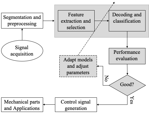
Figure 1: Basic parts of an offline BCI system. The pattern recognition parts are shaded.

The EEG temporal and spatial characteristics are correlated with an individual’s physical and mental state and may vary between subjects. Hence, subject-specific (SS) BCI models are designed and trained per subject, which makes SS BCI designs time consuming and inconvenient. To overcome the limitations of BCI, subject-independent (SI) BCI designs were introduced and received attention recently. The purpose of SI models is to train a general model that can be used by new subjects with little or no experimental calibration and model parameter adaptation.

Although MI EEG-based BCI is a major research area, it is not yet fully understood, possibly due to the lack of reliable data as well as complicated data collection and model training. Studies on SS BCI designs show that EEG classification on MI data has considerably lower accuracy than some other BCI tasks, such as P300, ERP, or VEP [4, 5]. For example, a recent study [6] reported a mean classification accuracy of $71.1\%$ for MI data, but $96.7\%$ and $95.1\%$ for the ERP and SSVEP paradigms. Mean accuracies of only $60.4\%$, $70.0\%$, and $67.4\%$ for MI EEG classification tasks were reported in [7, 8, 9], respectively. This can be partially attributed to the inability of the target users in operating the MI-related BCI system, also known as ”BCI-illiteracy” [7, 8, 10, 11]. The recent study in [6] reported an average BCI-illiteracy of 53.7% for the MI BCI paradigm, but 11.1% and 10.2% for ERP and SSVEP, respectively. BCI illiteracy can increase the number of outliers considerably, resulting in unreliable data.

On the other hand, SI BCI studies have reported variable classification accuracies. In [12, 13], maximum mean accuracies of $67\%$ and $72\%$ were reported, while in [14, 15] a comparison of the SS and SI BCI approaches reported an accuracy of $73\%$ and $64\%$ for the former, whereas the latter achieved $77\%$ and $68\%$ accuracy. The SI accuracy in [15] was increased to $84\%$ by considering various modifications, such as trial removal and partial inclusion of new user data in the training procedure.

Low classification accuracy can result in an inappropriate control signal and consequently make the MI EEG-based BCI system fail in either the SS or SI paradigms. BCI-illiteracy, lack of required experimentation, high between-subject variability, and small sample sizes can significantly contribute to low classification accuracy. Small sample size require the use of simple/linear statistical machine learning (ML) methods with few degrees of freedom [16]. However, even with simple ML methods, small sample size can pose issues due to the curse of dimensionality phenomenon [17, 18] and limitations in test-train split of the data, among many other issues [19, 20]. In addition, well-known methods like cross-validation may become inadmissible due to their high variance in MI EEG data-poor environments [21, 22, 23].

In this paper, we performed an empirical study of the classification accuracy of MI EEG-based SS and SI BCI designs, using Linear Discriminant Analysis (LDA), Support Vector Machines (SVM), Classification and regression tree (CART), and k-Nearest Neighbors (KNN), while investigating the effect of varying training sample size on classification accuracy. The rest of this paper is organized as follows. The basic classification methods and performance evaluation are described in Section II. Section III contains the experimental setups and results, which are discussed in Section IV. Finally, Section V contains conclusions.

II METHODS

II-A Sample Data

We used the publicly available MI EEG data provided by the GigaScience Repository [6]. 20 subjects (ages: 24-32 years) were seated in front of an LCD display, in a comfortable position, wearing a 62-channel EEG headset. Brain activity was recorded with a sampling rate of 1,000 Hz. The individuals were instructed to complete a in a single session a total of 40 trials: 20 left hand and 20 right hand imagery tasks.

Each trial started by displaying a ”+” symbol in the center of the screen which signaled the subjects to relax their muscles and prepare for the MI task. After 3 seconds, a right or left arrow was displayed and subjects performed the imagery task of grasping with the appropriate hand for 4 seconds. Subsequently, the screen turned black and subjects rested for 6 seconds. Trials were coded as a ”left” or ”right” class according to the displayed arrow. Figure 2 displays the study protocol for one trial.

Figure 2: Experimental design for a motor imagery trial.

II-B Pre-Processing

We restored the EEG signals from only the 20 channels that were placed on or close to the motor cortex [6]. Subsequently, we extracted the MI-specific segment of the signals, excluding a transitioning time between tasks. Then a Butterworth band-pass filter was applied to the signals to remove high-frequency noise and low-frequency artifacts and retain the brainwaves of interest [24], which include theta (deep relaxation and meditation state), alpha (relaxed, calm, and no-thinking state), and beta (awake and normal alert consciousness state).

II-C Feature Extraction and Selection

Studies have demonstrated that features based on the power spectral density (PSD) of MI EEG signals lead to consistent and robust pattern identification [25, 26, 27]. Let $x(t)$ be the EEG signal of a recording channel. The PSD of $x(t)$, which is defined in terms of the autocorrelation function $R_{XX}(\tau)$, is given by:

$$S_{xx}(\omega)=\int_{-\infty}^{+\infty}R_{xx}(\tau)e^{-i\omega\tau}d\tau\,.$$ (1)

The PSD is used to compute the signal power over given frequency ranges.

Since the autocorrelation function $R_{XX}(\tau)$ of the signal $x(t)$ is not known, we estimate the PSD per recording channel using the periodogram,

$$\hat{S}_{xx}(\omega)=\frac{\Delta t}{T}\left|\sum_{n=0}^{N-1}x[n]e^{-i\omega n\Delta t}\right|^{2}$$ (2)

where $x[n]=x(n\Delta t)$ is the discrete-time version of $x(t)$ using the sampling interval $\Delta t$.

To reduce the dimensionality, we selected the maximum of the periodogram over small intervals of 10 samples. Next, we appended the resulting values of the channels to create a feature vector. Finally, we performed a t-test to select the most discriminating features.

II-D Classification

Linear Discriminant Analysis (LDA) and Support Vector Machines (SVM) have been among the most popular parametric classification algorithms for EEG-based BCI system design [6, 28, 29, 30]. In particular, [31] highlighted that SVM has often outperformed other classifiers in the previous literature. In this section, we introduce some notation and briefly describe the LDA and SVM classification algorithms, as well as non-parametric classification algorithms, CART and k-NN.

A classifier assigns a label $y=\psi(\mathbf{x})$ to each feature vector $\mathbf{x}\in R^{d}$, where $y=0$ and $y=1$ indicate the ”right” and ”left” hand imagery tasks, respectively. The classifier is designed using training data by $S_{n}=\{\mathbf{X}_{1},Y_{1}),\ldots,(\mathbf{X}_{n},Y_{n})\}$, where $n$ is the sample size. Furthermore, $n_{0}$ and $n_{1}$ denote the sample sizes for class $y=0$ and $y=1$, respectively, with $n_{0}+n_{1}=n$.

II-D1 Linear Discriminant Analysis (LDA)

Assume that $p(\mathbf{x}\mid y\!=\!0)=N(\boldsymbol{\mu}_{0},\Sigma_{0})$ and $p(\mathbf{x}\mid y\!=\!1)=N(\boldsymbol{\mu}_{1},\Sigma_{1})$ are the class conditional densities for class $0$ and $1$, respectively. The unknown class means and covariance matrices are usually approximated by their maximum-likelihood estimators $\hat{\boldsymbol{\mu}}_{i}=\frac{1}{n_{i}}\sum_{j=1}^{n_{i}}\mathbf{X}_{j}I_{Y_{j}=i}$ and $\hat{\Sigma}_{i}=\frac{1}{n_{i}-1}\sum_{j=1}^{n_{i}}(\mathbf{X}_{j}-\hat{\boldsymbol{\mu}}_{i})(\mathbf{x}_{j}-\hat{\boldsymbol{\mu}}_{i})^{T}I_{Y_{j}=i}$, $i=0,1$, respectively. LDA makes the additional assumption that $\Sigma_{0}=\Sigma_{1}=\Sigma$, where the common covariance matrix $\Sigma$ can be estimated as

$$\hat{\Sigma}\,=\,\frac{1}{n_{0}+n_{1}-2}(n_{0}-1)\hat{\Sigma}_{0}+(n_{1}-1)\hat{\Sigma}_{0}\,.$$ (3)

The LDA classifier corresponds to plugging in the aforementioned parameter esimtators in the expression for the optimal classifier under the Gaussian distributional assumption, which yields

$$\psi_{n}(\mathbf{x})\,=\,\left\{\begin{array}[]{ll}1,&\mathbf{w}^{T}\mathbf{x}+b>0,\\ 0,&\textrm{otherwise},\end{array}\right.$$ (4)

where

$$\begin{array}[]{l}\mathbf{w}\,=\,\hat{\Sigma}^{-1}(\hat{\boldsymbol{\mu}_{1}}-\hat{\boldsymbol{\mu}_{0}})\,,\\ b\,=\,\frac{1}{2}(\hat{\boldsymbol{\mu}_{1}}-\hat{\boldsymbol{\mu}_{0}})^{T}\hat{\Sigma}^{-1}(\hat{\boldsymbol{\mu}_{0}}+\hat{\boldsymbol{\mu}_{1}})\,.\end{array}$$ (5)

II-D2 Support Vector Machine (SVM)

Linear SVM is a linear discriminant with maximum margins, i.e., maximum separation between the decision boundary and the training data. It can be shown that the margin is given by $\frac{1}{||\mathbf{w}||}$ and one needs to maximize that. The margin constraints can be written, Without loss of generality, as $\mathbf{w}\mathbf{X}_{j}+b\geq 1$ or $\mathbf{w}\mathbf{X}_{j}+b\leq 1$, depending on whether $Y_{j}=1$ or $Y_{j}=-1$, respectively, for $j=1,\ldots,n$ (class “0” here is coded by $-1$). Hence, one obtains a convex optimization problem

$$\begin{array}[]{l}\mbox{minimize}\ \ \ \frac{1}{2}||\mathbf{w}||^{2}\\[4.30554pt] \mbox{subject to }\ \ Y_{i}(\mathbf{w}^{T}\mathbf{X}_{i}+b)>0,\ j=1,\ldots,n.\end{array}$$ (6)

the solution of which is given by

$$\begin{array}[]{l}\mathbf{w}^{*}\,=\,\sum_{j\in\mathcal{S}}\lambda_{j}^{*}Y_{j}\mathbf{X}_{j}\,,\\[4.30554pt] b^{*}\,=\,-\frac{1}{n}\sum_{j\in\mathcal{S}}\sum_{k\in\mathcal{S}}\lambda_{j}^{*}Y_{j}\mathbf{X}_{j}^{T}\mathbf{X}_{k}+\frac{1}{n}\sum_{j\in\mathcal{S}}Y_{j}\end{array}$$ (7)

where $\lambda_{j}^{*}$ are the optimal values of the Lagrange multipliers for the preceding optimization problem, for $j=1,\ldots,n$, and $\mathcal{S}$ is the set of indices of the support vectors, i.e., training points $(\mathbf{X}_{j},Y_{j})$ for which $\lambda_{j}>0$. The LSVM classifier is then given by:

$$\psi_{n}(\mathbf{x})\,=\,\left\{\begin{array}[]{ll}1,&(\mathbf{w}^{*})^{T}\mathbf{x}+b^{*}>0,\\ -1,&\textrm{otherwise},\end{array}\right.$$ (8)

In practice, slack variables are introduced into the optimization problem to allow points to violate the margin, allowing the solution of nonlinearly separable problems and avoiding overfitting.

A non-linear SVM replaces all dot-products $\mathbf{x}^{T}\mathbf{x}^{\prime}$ in the linear SVM formulation by a kernel function $k(\mathbf{x},\mathbf{x}^{\prime})=\Phi(\mathbf{x})^{T}\Phi(\mathbf{x}^{\prime})$. This correponds to transforming the data to a higher-dimensional space using $\Phi$ and applying a linear SVM to the transformed data. Here we use the radial basis function (RBF) kernel,

$$k(\mathbf{x},\mathbf{x}^{\prime})\,=\,\exp\left(\frac{||\mathbf{x}-\mathbf{x}^{\prime}||^{2}}{2\sigma^{2}}\right)$$ (9)

where $\sigma$ is the kernel bandwidth parameter and is estimated from the observed data.

II-D3 Classification and regression tree (CART)

CART is a non-parametric decision tree algorithm. At each node of the tree, CART sets a threshold on a selected feature to split the data into two groups. The threshold and feature are selected at each node such that the impurity of the children nodes is minimized. At a terminal node, or leaf node, a label is assigned according to majority vote among the training points in the leaf node. To avoid overfitting, node splitting is usually terminated early.

II-D4 K nearest neighbors (kNN)

kNN is another non-parametric classification algorithm. At any point in the feature space, kNN assigns the majority label among the k nearest training points. Smoothness of the kNN classifier decision boundary increases as k increases. Too small $k$ (say $k=1$) introduces overfitting, but too large $k$ leads to underfitting. To avoid ties, odd $k$ is recommended in binary classification problems.

III EXPERIMENTAL RESULTS

We report in this section the results of a comprehensive empirical comparison of the previous classification algorithms on the MI EEG data described earlier.

Similarly to [6], to account for the transition time, we removed the first 1s and last 0.5s of the MI segments of the EEG signals and performed the rest of the analysis on the middle 2.5 seconds. The signals were filtered using a Butterworth band-pass filter with lower and upper cut-off frequencies of 3 and 35 Hz, respectively. The p-value threshold for the t-test was set to $0.05$ for the SS model, which resulted in various numbers of selected features per subject. This threshold was set on $0.005$ for the SI experiments, which resulted in total of 29 features.

We performed several classification experiments using the LDA, RB-SVM, CART, and kNN classification algorithms. We set the minimum leaf size to 3 for CART and $k=3$ for kNN. Classifier generalization ability was evaluated by randomly splitting the available data into 50% training data $S_{N}$ and 50% testing data $S_{M}$, and using a test-set error estimator, which is the relative accuracy of the trained classifier on the testing set. In our SI design, the total sample size was $800$, so that the testing sample size was $400$, which is enough to guarantee excellent test-set error estimation accuracy [32].

For the training step, $n\leq 400$ sample points were randomly drawn from $S_{N}$. For each value of $n$, we trained the classifiers on the selected data, calculated the test set error on $S_{M}$, and finally computed the percent prediction accuracies as $100(1-\mbox{test set error})\%$. The classification performances was examined with $n\in\{10,15,20\}$ for the SS and $n\in\{100,150,200,250,300,350,400\}$ for the SI models.

Randomly drawn training samples introduces a randomness factor to the classifiers’ training and prediction performance. To take into account this randomness factor, we repeated each experimental case 100 times. The SS models’ performance are presented in Table I and Figures 3 and 5. Table II shows the mean (std) percent accuracy of the SI models, whereas figure 6 compares the mean accuracy of the four classifiers for varying training sample sizes, ranging from $n=100$ to $n=400$. Figure 7 displays box plots of classifier accuracy for SI and SS approaches and compares the mean accuracy and standard deviation for varying training sample size.

Subject	LDA			SVM			CART			k-NN			$\Psi$ with highest mean accuracy
	n=10	n=15	n=20	n=10	n=15	n=20	n=10	n=15	n=20	n=10	n=15	n=20	n=10	n=15	n=20
S1	69	72	73	59	63	71	77	77	80	63	61	69	CART	CART	CART
S2	67	70	70	56	67	72	66	71	78	67	68	68	LDA	CART	CART
S3	51	54	53	57	62	71	52	57	61	52	56	56	SVM	SVM	SVM
S4	71	71	73	63	60	73	67	68	74	68	72	79	LDA	k-NN	k-NN
S5	57	59	65	64	69	79	64	66	66	64	67	76	SVM	SVM	SVM
S6	75	78	80	59	64	72	74	75	80	65	70	70	LDA	LDA	LDA
S7	76	80	84	57	61	68	68	71	75	61	65	78	LDA	LDA	LDA
S8	86	91	88	56	63	72	82	84	86	83	86	87	LDA	LDA	LDA
S9	68	77	81	59	65	73	69	72	75	65	67	64	CART	LDA	LDA
S10	70	74	82	57	64	73	71	73	79	67	72	77	LDA	LDA	LDA
S11	67	70	73	70	76	83	74	76	77	67	72	72	CART	CART	SVM
S12	65	71	78	57	65	64	64	67	72	59	59	57	LDA	LDA	LDA
S13	83	79	82	54	64	64	79	88	94	87	89	91	k-NN	k-NN	CART
S14	73	80	83	60	62	67	73	74	80	78	80	81	k-NN	LDA	LDA
S15	85	86	91	62	69	78	93	95	98	88	93	94	CART	CART	CART
S16	77	80	86	59	65	75	77	77	85	76	81	81	LDA	k-NN	LDA
S17	69	70	78	62	66	77	68	74	80	71	81	87	k-NN	k-NN	k-NN
S18	77	75	74	59	60	66	76	78	88	67	70	74	LDA	CART	CART
S19	72	76	82	62	66	68	70	72	77	62	69	71	LDA	LDA	LDA
S20	66	66	71	64	65	72	65	69	81	63	63	68	LDA	CART	CART
mean	71	74	77	60	65	72	71	74	79	69	72	75
std	9	8	9	4	4	5	8	8	8	9	10	10

TABLE I: Mean accuracy in percentage per subject for SS models with three sample sizes $n$. Numbers are rounded to the closest integer. Last three columns show the classification algorithm with the highest mean accuracy per subject per sample size.

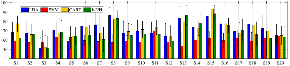
Figure 3: Barplots of the mean accuracy in SS models with $n=10$. The error bars display the standard deviations.

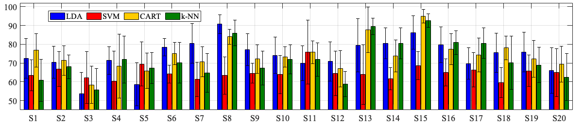
Figure 4: Barplots of the mean accuracy in SS models with $n=15$. The error bars display the standard deviations.

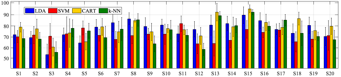
Figure 5: Barplots of the mean accuracy in SS models with $n=20$. The error bars display standard deviations.

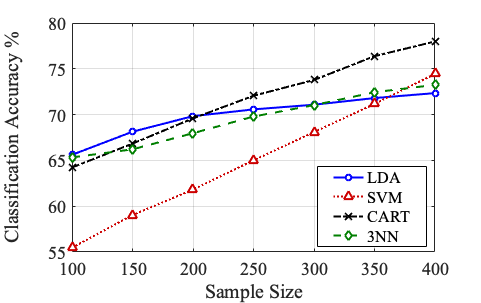
Figure 6: Comparison of the mean accuracy for SI models.

$n$	LDA	SVM	CART	k-NN	Max(acc)
100	66 (3)	55 (2)	65 (2)	66 (3)	LDA
150	69 (2)	59 (1)	68 (3)	66 (2)	LDA
200	69 (2)	62 (1)	71 (3)	69 (2)	CART
250	71 (2)	65 (1)	72 (3)	70 (2)	CART
300	72 (2)	68 (1)	74 (2)	72 (2)	CART
350	72 (1)	71 (1)	77 (3)	73 (2)	CART
400	73 (1)	74 (1)	78 (2)	74 (1)	CART

TABLE II: The mean (std) accuracies in percentage for subject independent models. The last column shows the classification algorithm with the highest test-set prediction accuracy.

Subject-independent	Subject-specific

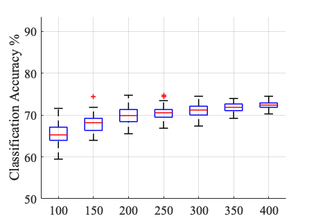
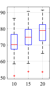
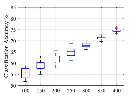
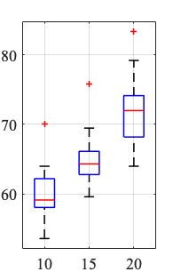
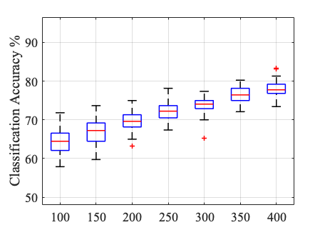
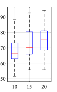
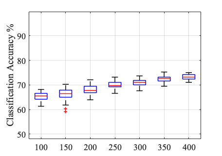
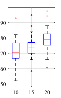
Figure 7: Box plots for prediction accuracies of SI (left) and SS (right) designs, with classification algorithms: LDA (1^st row), SVM (2^nd row), CART (3^rd row), and 3-NN (4^th row). Horizontal axis shows sample size.

IV DISCUSSION

Our experiments lead to several interesting conclusions. For SI design, as displayed in figure 6, in the small sample-size region ($100\leq n\leq 200$), LDA was the best performing classifier. CART beats all other classifiers if $200\leq n\leq 400$ samples are provided. SVM was the most robust (lowest std) in both SS and SI paradigms. The steep improvement in SVM accuracy leads to the hypothesis that it may achieve the highest accuracy if the training sample size is large enough.

For the SS design, as illustrated by Figures 3 - 5 and Table I, increasing sample size improves the classification performance in terms of mean prediction accuracy, although it may be impracticable to collect many EEG recordings per subject. While SVM was the best performing classifier for only a few subjects (S3, S5, and S11 when n=20), the other three classifiers compete for the highest SS accuracy. This behaviour suggests a hypothesis that a hybrid model may be beneficial for SS BCI systems, where a specific classification algorithm is selected according to the maximum accuracy of the test set for that single individual.

The side-by-side box plots in figures 7 show that, for all classification algorithms, in contrast to the SI models, the variance of the trained SS classifiers is not reduced with an increment in training sample size. Indeed, the variance is increased noticeably in CART and SVM. This variability is expected at least due to the high between-subject differences in EEG signals, and suggests that a trained BCI may not be appropriate for a totally new user. It is worthy to note that the study in [15] also demonstrated improved accuracy by including a few samples from new users in training a SI BCI.

Overall, the results indicate that SS designs, and possibly a hybrid SS model, may be more appropriate for personalized MI BCI if collecting enough samples from a specific subject is feasible. In case a recording session is inconvenient for a subject, particularly for mentally or physically challenged people, a SI BCI may be used. Such SI BCI should be trained on a sufficiently large training data set that is collected from a large group of subjects covering between-subject variability. Comparing the box plots, it can be seen that classification mean accuracy in SI BCI even with a relatively large sample size ($n=400$) is close to that of SS BCI with $n=20$. However, the low variance of SI BCI acccuracy may make it more applicable for a multi-user system.

V CONCLUSIONS

This paper presents our evaluation of the subject-specific (SS) and subject-independent (SI) paradigms using two popular classification algorithms in MI BCI design, LDA and SVM, in addition to the non-parametric algorithms k-NN and CART. Our results show that for SI BCI, LDA beats other classification algorithms in the presence of small sample size. CART outperforms the rest for a relatively large sample size, whereas we hypothesize that SVM achieves the highest accuracy with a sufficiently large sample size. It is important to stress that generalization performance should be evaluated on a relatively large and independent test set, which was done here.

For SS models, although LDA and CART performed well for majority of subjects, the best classifier performance depends on the subject, which suggests the applicability of a hybrid model. As was demonstrated in[33] for gender-specific BCIs, considering the subject gender may improve the performance of SI designs. We leave the investigation of gender-specific SI BCI performance to future work. Another interesting research problem is to investigate the EEG recording channels with the least discriminating information, for example by using a sequential backward search. In addition, deep learning methods, particularly convolutional neural networks (CNNs), are able to process brain maps as input images, but may need larger sample size for training a network with good generalization abilities. A future experiment may study the performance of CNNs for SI BCI considering varying sample sizes.

References

- [1] G. Pfurtscheller and C. Neuper, “Motor imagery and direct brain-computer communication,” Proceedings of the IEEE, vol. 89, no. 7, pp. 1123–1134, 2001.
- [2] M. Jeannerod, “Mental imagery in the motor context,” Neuropsychologia, vol. 33, no. 11, pp. 1419–1432, 1995.
- [3] J. Decety, D. Perani, M. Jeannerod, V. Bettinardi, B. Tadary, R. Woods, J. C. Mazziotta, and F. Fazio, “Mapping motor representations with positron emission tomography,” Nature, vol. 371, no. 6498, pp. 600–602, 1994.
- [4] J. Kevric and A. Subasi, “Comparison of signal decomposition methods in classification of eeg signals for motor-imagery bci system,” Biomedical Signal Processing and Control, vol. 31, pp. 398–406, 2017.
- [5] C. Guger, S. Daban, E. Sellers, C. Holzner, G. Krausz, R. Carabalona, F. Gramatica, and G. Edlinger, “How many people are able to control a p300-based brain–computer interface (bci)?” Neuroscience letters, vol. 462, no. 1, pp. 94–98, 2009.
- [6] M.-H. Lee, O.-Y. Kwon, Y.-J. Kim, H.-K. Kim, Y.-E. Lee, J. Williamson, S. Fazli, and S.-W. Lee, “Eeg dataset and openbmi toolbox for three bci paradigms: an investigation into bci illiteracy,” GigaScience, vol. 8, no. 5, p. giz002, 2019.
- [7] C. Guger, G. Edlinger, W. Harkam, I. Niedermayer, and G. Pfurtscheller, “How many people are able to operate an eeg-based brain-computer interface (bci)?” IEEE transactions on neural systems and rehabilitation engineering, vol. 11, no. 2, pp. 145–147, 2003.
- [8] M. Ahn, H. Cho, S. Ahn, and S. C. Jun, “High theta and low alpha powers may be indicative of bci-illiteracy in motor imagery,” PloS one, vol. 8, no. 11, p. e80886, 2013.
- [9] H. Cho, M. Ahn, S. Ahn, M. Kwon, and S. C. Jun, “Eeg datasets for motor imagery brain–computer interface,” GigaScience, vol. 6, no. 7, p. gix034, 2017.
- [10] C. Vidaurre and B. Blankertz, “Towards a cure for bci illiteracy,” Brain topography, vol. 23, no. 2, pp. 194–198, 2010.
- [11] L. F. Nicolas-Alonso and J. Gomez-Gil, “Brain computer interfaces, a review,” sensors, vol. 12, no. 2, pp. 1211–1279, 2012.
- [12] B. Reuderink, J. Farquhar, M. Poel, and A. Nijholt, “A subject-independent brain-computer interface based on smoothed, second-order baselining,” in 2011 Annual International Conference of the IEEE Engineering in Medicine and Biology Society. IEEE, 2011, pp. 4600–4604.
- [13] E. Dong, C. Yue, and S. Du, “Classification of subject-independent motor imagery eeg based on relevance vector machine,” in 2020 IEEE International Conference on Mechatronics and Automation (ICMA). IEEE, 2020, pp. 67–71.
- [14] F. Lotte, C. Guan, and K. K. Ang, “Comparison of designs towards a subject-independent brain-computer interface based on motor imagery,” in 2009 Annual International Conference of the IEEE Engineering in Medicine and Biology Society. IEEE, 2009, pp. 4543–4546.
- [15] S. M. Hosseini, M. Bavafa, and V. Shalchyan, “An auto-adaptive approach towards subject-independent motor imagery bci,” in 2019 26th National and 4th International Iranian Conference on Biomedical Engineering (ICBME). IEEE, 2019, pp. 167–171.
- [16] P. Ghane and G. Hossain, “Learning patterns in imaginary vowels for an intelligent brain computer interface (bci) design,” arXiv preprint arXiv:2010.12066, 2020.
- [17] M. Verleysen and D. François, “The curse of dimensionality in data mining and time series prediction,” in International work-conference on artificial neural networks. Springer, 2005, pp. 758–770.
- [18] G. V. Trunk, “A problem of dimensionality: A simple example,” IEEE Transactions on pattern analysis and machine intelligence, no. 3, pp. 306–307, 1979.
- [19] A. Golugula, G. Lee, and A. Madabhushi, “Evaluating feature selection strategies for high dimensional, small sample size datasets,” in 2011 Annual International conference of the IEEE engineering in medicine and biology society. IEEE, 2011, pp. 949–952.
- [20] A. Jain and D. Zongker, “Feature selection: Evaluation, application, and small sample performance,” IEEE transactions on pattern analysis and machine intelligence, vol. 19, no. 2, pp. 153–158, 1997.
- [21] R. Kohavi et al., “A study of cross-validation and bootstrap for accuracy estimation and model selection,” in Ijcai, vol. 14, no. 2. Montreal, Canada, 1995, pp. 1137–1145.
- [22] G. Varoquaux, “Cross-validation failure: small sample sizes lead to large error bars,” Neuroimage, vol. 180, pp. 68–77, 2018.
- [23] U. M. Braga-Neto and E. R. Dougherty, “Is cross-validation valid for small-sample microarray classification?” Bioinformatics, vol. 20, no. 3, pp. 374–380, 2004.
- [24] P. Ghane, G. Hossain, and A. Tovar, “Robust understanding of eeg patterns in silent speech,” in 2015 National Aerospace and Electronics Conference (NAECON). IEEE, 2015, pp. 282–289.
- [25] V. P. Oikonomou, K. Georgiadis, G. Liaros, S. Nikolopoulos, and I. Kompatsiaris, “A comparison study on eeg signal processing techniques using motor imagery eeg data,” in 2017 IEEE 30th international symposium on computer-based medical systems (CBMS). IEEE, 2017, pp. 781–786.
- [26] P. Herman, G. Prasad, T. M. McGinnity, and D. Coyle, “Comparative analysis of spectral approaches to feature extraction for eeg-based motor imagery classification,” IEEE Transactions on Neural Systems and Rehabilitation Engineering, vol. 16, no. 4, pp. 317–326, 2008.
- [27] N. Brodu, F. Lotte, and A. Lécuyer, “Comparative study of band-power extraction techniques for motor imagery classification,” in 2011 IEEE Symposium on Computational Intelligence, Cognitive Algorithms, Mind, and Brain (CCMB). IEEE, 2011, pp. 1–6.
- [28] F. Lotte, L. Bougrain, A. Cichocki, M. Clerc, M. Congedo, A. Rakotomamonjy, and F. Yger, “A review of classification algorithms for eeg-based brain–computer interfaces: a 10 year update,” Journal of neural engineering, vol. 15, no. 3, p. 031005, 2018.
- [29] P. Ghane, “Silent speech recognition in eeg-based brain computer interface,” Ph.D. dissertation, 2015.
- [30] L. Sarmiento, P. Lorenzana, C. Cortes, W. Arcos, J. Bacca, and A. Tovar, “Brain computer interface (bci) with eeg signals for automatic vowel recognition based on articulation mode,” in 5th ISSNIP-IEEE Biosignals and Biorobotics Conference (2014): Biosignals and Robotics for Better and Safer Living (BRC). IEEE, 2014, pp. 1–4.
- [31] F. Lotte, M. Congedo, A. Lécuyer, F. Lamarche, and B. Arnaldi, “A review of classification algorithms for eeg-based brain–computer interfaces,” Journal of neural engineering, vol. 4, no. 2, p. R1, 2007.
- [32] U. Braga-Neto and E. Dougherty, Error Estimation for Pattern Recognition. New York: Wiley, 2015.
- [33] J. Cantillo-Negrete, J. Gutierrez-Martinez, R. I. Carino-Escobar, P. Carrillo-Mora, and D. Elias-Vinas, “An approach to improve the performance of subject-independent bcis-based on motor imagery allocating subjects by gender,” Biomedical engineering online, vol. 13, no. 1, p. 158, 2014.