A Principle Solution for Enroll-Test Mismatch in Speaker Recognition

Abstract

Mismatch between enrollment and test conditions causes serious performance degradation on speaker recognition systems. This paper presents a statistics decomposition (SD) approach to solve this problem. This approach decomposes the PLDA score into three components that corresponding to enrollment, prediction and normalization respectively. Given that correct statistics are used in each component, the resultant score is theoretically optimal. A comprehensive experimental study was conducted on three datasets with different types of mismatch: (1) physical channel mismatch, (2) speaking behavior mismatch, (3) near-far recording mismatch. The results demonstrated that the proposed SD approach is highly effective, and outperforms the ad-hoc multi-condition training approach that is commonly adopted but not optimal in theory.

I Introduction

Speaker recognition has been emerging as an applicable technique after decades of research [1, 2, 3]. Traditional speaker recognition methods are based on statistical models, in particular the Gaussian mixture model-universal background model (GMM-UBM) [4] and the subspace alternatives including joint factor analysis (JFA) [5] and the i-vector model [6]. Recently, deep learning methods have demonstrated significant progress with regard to speaker recognition [7]. Early research learns frame-level features and derives utterance-level representations by simple average [8, 9], and the following research focuses on deriving utterance-level representations directly [10, 11]. The utterance-level representations are often called speaker vectors, and the process that maps a variant-length speech signal to a fixed-dimension speaker vector is often called speaker embedding. As far, the most popular deep learning architecture for speaker embedding is the x-vector model, proposed by Snyder et al. [10]. Compared to an alternative deep learning approach that employs an end-to-end architecture and training scheme [12, 13, 14], the embedding approach is easier to train [15] and the derived speaker vectors can support various speaker-related tasks. Recent progress on the deep speaker embedding approach includes more comprehensive architecture [16, 17], improved pooling methods [11, 18, 19, 20], better training criteria [21, 22, 23, 24, 25, 26], and better training schemes [27, 28, 29].

In spite of the tremendous progress, the present speaker recognition performance yet cannot meet the request of real applications. A particular problem is that the performance of a model trained with data from one domain will be substantially reduced when applied to another domain. Numerous studies have been carried out to deal with the domain-mismatch problem [30, 31, 32, 33, 34, 35, 36, 37, 38, 39, 40]. Most of the research focuses on domain drift, and the central idea is to build statistical models suitable for the target domain, by using the knowledge of data or model of the source domain. These techniques are suitable for solving the mismatch between the training data and the deployment environment. For example, they can adapt a model trained with a large database of reading speech so as to make it applicable in a new scenario of online meetings.

In this paper, we focus on another mismatch issue that seems more serious: the mismatch between the enrollment and test conditions. In real applications, the condition of enrollment is often controlled: people tend to speak in the same acoustic environment and in the same manner, and also the recording device does not change. During test, the condition tends to be much more uncontrollable and unpredictable. It is often significantly different from the enrollment condition, and varies from one test to another. Significant performance reduction is often observed with this mismatch [41, 42, 43, 44]. Some typical scenarios that involve serious enrollment-test mismatch are:

• Cross-Channel test, where the enrollment uses one device and the test uses another device. This leads to clear mismatch on the recording devices.

• Time-Variance test, where the test is conducted in a few weeks or months after the enrollment. This leads to significant mismatch on the speaking behaviors.

• Near-Far field test, where the enrollment uses a near-filed microphone while the test uses a far-field microphone, or vice versa. This leads to clear mismatch on the recording conditions.

More complex situations may involve multiple mismatches. For example, in the multi-genre scenarios, the speaker may enroll in reading speech with a near electret microphone, while the test could be in chatting or singing, with a far-field dynamic microphone.

The essential problem associated with this enrollment-test mismatch is that the statistical properties (e.g., between-speaker variance and within-speaker variance) of the enrollment data and the test data are different, which we call statistics incoherence. This incoherence fails most of the scoring models, e.g., the famous probabilistic linear discriminant analysis (PLDA) [45, 46], for which statistics coherence between enrollment and test is a prerequisite.

Inter-dataset variability compensation (IDVC) [37] and joint PLDA [47, 48] model speaker and condition as two variables, and compensate for the variance associated with condition during the inference. In particular, joint PLDA can compensate for enrollment-test mismatch by specifying that the conditions of the enrollment and test are different. These factorization models rely on multi-conditional data to separate the variations associated with speaker and condition, which is not possible for a particular enrollment-test condition pair where the condition factor could be vague. Moreover, the compensation does not fully utilize the statistical information in each condition, so is only partial.

Another commonly used approach in practice is score calibration [49, 50, 51]. This approach normalizes the score distribution according to the test condition, making the decision robust to condition change. For a particular enrollment-test condition pair, however, calibration does not improve the discriminant capacity of the score.

This paper will present a novel solution for the enrollment-test mismatch problem, especially for a particular enrollment-test condition pair. The solution decomposes the PLDA score into three components: enrollment, prediction, and normalization. By this composition, different statistical models can be used for different components. If we use the statistics of the enrollment condition for the enrollment component, and the statistics of the test condition for the prediction and normalization components, the resultant PLDA score remains sound even if the enrollment and test conditions are mismatched. We call this approach statistics decomposition (SD). It is a principle solution for the enrollment-test mismatch problem, as the resultant score is optimal if the statistics on the enrollment and test conditions are both accurate, even if they are not coherent.

The rest of the paper is organized as follows. Section II will present a theoretical background by revisiting the PLDA model, especially the decomposition form. Section III presents the SD approach for the enrollment-test mismatch problem based on a simple linear transformation. Experiments are reported in Section V, and finally the paper is concluded in Section VI.

II Theory background

II-A Revisit PLDA

Giving some speaker vectors $\boldsymbol{x}_{1},\boldsymbol{x}_{2},..,\boldsymbol{x}_{n}$ for enrollment and a speaker vector $\boldsymbol{x}$ for test, the task of speaker verification is to check which of the following two hypotheses is more probable:

• $H_{0}$: $\boldsymbol{x}$ and $\boldsymbol{x}_{1},\boldsymbol{x}_{2},..,\boldsymbol{x}_{n}$ are produced from the same speaker class;

• $H_{1}$: $\boldsymbol{x}$ and $\boldsymbol{x}_{1},\boldsymbol{x}_{2},..,\boldsymbol{x}_{n}$ are produced from different speaker classes.

Following the Bayes theory, decisions based on the following log likelihood ratio (LLR) are optimal, in terms of minimum Bayes risk (MBR):

$$\text{LLR}=\log\frac{p(\boldsymbol{x},\boldsymbol{x}_{1},...,\boldsymbol{x}_{n}|H_{0})}{p(\boldsymbol{x},\boldsymbol{x}_{1},...,\boldsymbol{x}_{n}|H_{1})}.$$ (1)

Applying the assumptions of $H_{0}$ and $H_{1}$, the LLR score can be written as follows:

$$\text{LLR}=\log\frac{p(\boldsymbol{x},\boldsymbol{x}_{1},...,\boldsymbol{x}_{n})}{p(\boldsymbol{x})p(\boldsymbol{x}_{1},...,\boldsymbol{x}_{n})},$$ (2)

where $p(\boldsymbol{x}_{1},\boldsymbol{x}_{2},...,\boldsymbol{x}_{n})$ is the joint probability of $\boldsymbol{x}_{1},\boldsymbol{x}_{2},...,\boldsymbol{x}_{n}$ under the assumption that they are from the same speaker. Note that the numerator can not be factorized further as the variables are from the same speaker and so are dependent on each other.

PLDA assumes a linear Gaussian model for the generation process of $\boldsymbol{x}$, where both the between-class and within-class distributions are Gaussians. In this work, we assume that both the between-speaker and within-speaker covariances are full-rank, which is known as a two-covariance model [52]. More discussion about this special form and other PLDA variants can be found in [53].

To simplify the presentation, we further assume that a linear transformation has been applied to the data so both the between-speaker and within-speaker covariances are diagonal. Moreover, we will use the isotropic form for both the two covariances in the following formulation. In practice, the usual case is that at least one of the covariances is non-isotropic, but the formulation is very similar to the all-isotropic form presented below.

Let $\boldsymbol{\mu}$ denote the class mean, the PLDA model, in the form of two isotropic covariances, can be written as follows:

$$p(\boldsymbol{\mu})=N(\boldsymbol{\mu};\boldsymbol{0},\epsilon\mathbf{I});$$ (3)

$$p(\boldsymbol{x}|\boldsymbol{\mu})=N(\boldsymbol{x};\boldsymbol{\mu},\sigma\mathbf{I}),$$ (4)

where $\epsilon$ and $\sigma$ are the between-speaker variance and the within-speaker variance, respectively.

With this model, it is easy to derive the marginal probability $p(\boldsymbol{x})$ as follows:

$$p(\boldsymbol{x})=N(\boldsymbol{x};\boldsymbol{0},(\epsilon+\sigma)\mathbf{I}),$$ (5)

and the marginal probability for multiple vectors of a single speaker can be obtained as follows:

$$p(\boldsymbol{x}_{1},...,\boldsymbol{x}_{n}) \propto\exp\big{\{}-\frac{1}{2\sigma}\{\sum_{i}||\boldsymbol{x}_{i}||^{2}-\frac{n^{2}\epsilon}{\sigma+n\epsilon}||\bar{\boldsymbol{x}}||^{2}\}\big{\}}.$$ (6)

With this marginal, it is easy to compute LLR according to Eq.(2).

II-B Decomposition form of PLDA

The LLR score can be formulated into a decomposition form [54, 55, 56, 57, 58] as follows:

LLR $$= \log\frac{p(\boldsymbol{x}|\boldsymbol{x}_{1},...,\boldsymbol{x}_{n})}{p(\boldsymbol{x})}$$ (7)

$$= \log\int p(\boldsymbol{\mu}|\boldsymbol{x}_{1},...,\boldsymbol{x}_{n})p(\boldsymbol{x}|\boldsymbol{\mu})\,\rm{d}{\boldsymbol{\mu}}-\log\mathit{p}(\boldsymbol{x}).$$

By this formulation, the LLR scoring can be separated to three phases:

• Enrollment: Compute the posterior $p(\boldsymbol{\mu}|\boldsymbol{x}_{1},\boldsymbol{x}_{2},...,\boldsymbol{x}_{n})$.

• Prediction: Compute the likelihood $p_{k}(\boldsymbol{x})=\int p(\boldsymbol{\mu}|\boldsymbol{x}_{1},\boldsymbol{x}_{2},...,\boldsymbol{x}_{n})p(\boldsymbol{x}|\boldsymbol{\mu})\rm{d}{\boldsymbol{\mu}}$.

• Normalization: Compute the normalization term $p(\boldsymbol{x})$ and use it to normalize the likelihood by $\log p_{k}(\boldsymbol{x})-\log p(\boldsymbol{x})$.

This decomposition offers an intuitive interpretation for the LLR score, and simplifies the computation. According to the PLDA model, the posterior for $\boldsymbol{\mu}$ is computed as follows:

$$p(\boldsymbol{\mu}|\boldsymbol{x}_{1},...,\boldsymbol{x}_{n})=N(\boldsymbol{\mu};\frac{n\epsilon}{n\epsilon+\sigma}\bar{\boldsymbol{x}},\frac{\epsilon\sigma}{n\epsilon+\sigma}\mathbf{I}),$$ (8)

where $\bar{\boldsymbol{x}}$ is the average of the observations $\boldsymbol{x}_{1},...,\boldsymbol{x}_{n}$. The likelihood $p(\boldsymbol{x}|\boldsymbol{x}_{1},...,\boldsymbol{x}_{n})$ can therefore be computed by marginalizing over $\boldsymbol{\mu}$:

$$p(\boldsymbol{x}|\boldsymbol{x}_{1},...,\boldsymbol{x}_{n}) = \int p(\boldsymbol{x}|\boldsymbol{\mu})p(\boldsymbol{\mu}|\boldsymbol{x}_{1},...,\boldsymbol{x}_{n})\rm{d}\boldsymbol{\mu}$$ (9)

$$= N(\boldsymbol{x};\frac{n\epsilon}{n\epsilon+\sigma}\bar{\boldsymbol{x}},(\sigma+\frac{\epsilon\sigma}{n\epsilon+\sigma})\mathbf{I}).$$

A simple computation shows that:

LLR $$= \log p(\boldsymbol{x}|\boldsymbol{x}_{1},...,\boldsymbol{x}_{n})-\log p(\boldsymbol{x})$$

$$\propto -\frac{1}{\sigma+\frac{\epsilon\sigma}{n\epsilon+\sigma}}||\boldsymbol{x}-\tilde{\boldsymbol{\mu}}||^{2}+\frac{1}{\epsilon+\sigma}||\boldsymbol{x}||^{2},$$

where we have defined:

$$\tilde{\boldsymbol{\mu}}=\frac{n\epsilon}{n\epsilon+\sigma}\bar{\boldsymbol{x}}.$$ (11)

III Statistics Decomposition

In this section, we employ the decomposition form of PLDA to address enrollment-test mismatch. Note that the essential problem in the enrollment-test mismatch scenario is that the statistics of the enrollment and test conditions are incoherent, and so require different models to represent each of them. The standard form of PLDA LLR involves the enrollment and test data in a single model, as evidenced by the joint likelihood $p(\boldsymbol{x},\boldsymbol{x}_{1},...,\boldsymbol{x}_{n})$. This makes it unsuitable for dealing with enrollment-test mismatch. In contrast, the decomposition form decouples the scoring process into separate phases, and each phase can use its own (and correct) statistical model. This offers a principle solution for the enrollment-test mismatch problem, which we call statistics decomposition (SD).

III-A General form

With the SD approach, it is clear that the enrollment and normalization phases should be based on the statistics of the enrollment and test condition, respectively. The prediction phase, however, it is more complex. According to Eq.(7), it marginalizes the conditional probability $p(\boldsymbol{x}|\boldsymbol{\mu})$ with respect to the posterior $p(\boldsymbol{\mu}|\boldsymbol{x}_{1},...,\boldsymbol{x}_{n})$. However, $p(\boldsymbol{\mu}|\boldsymbol{x}_{1},...,\boldsymbol{x}_{n})$ is computed based on the statistical model of the enrollment condition, and so is not a correct posterior for marginalizing the conditional probability $p(\boldsymbol{x}|\boldsymbol{\mu})$ where $\boldsymbol{\mu}$ and $\boldsymbol{x}$ are quantities in the test condition.

In order to solve this problem, a connection must be established between the quantities in the enrollment condition and the test condition. A possible solution is to design a mapping function that transforms $\boldsymbol{\mu}$ from the enrollment condition to the test condition, or vice versa, transforms $\boldsymbol{x}$ from the test condition to the enrollment condition. In this study, we will choose the transformation on $\boldsymbol{x}$, as it results in a relatively simpler form. For simplicity, we shall assume that the transformation is linear:

$$\boldsymbol{x}=\mathbf{M}\hat{\boldsymbol{x}}+\boldsymbol{b},$$ (12)

where $\hat{\boldsymbol{x}}$ represents the observation in the test condition, and $\boldsymbol{x}$ is the transformed data in the enrollment condition. If we assume that the transformed data can be well represented by the statistical model of the enrollment condition, the LLR score can be derived.

Firstly, denote the enrollment data of the $k$-th class by $\boldsymbol{x}^{k}_{1},...,\boldsymbol{x}^{k}_{n_{k}}$. According to Eq. (8), the posterior $p(\boldsymbol{\mu}_{k}|\boldsymbol{x}^{k}_{1},...,\boldsymbol{x}^{k}_{n_{k}})$ is computed using the model of the enrollment condition:

$$p(\boldsymbol{\mu}_{k}|\boldsymbol{x}^{k}_{1},...,\boldsymbol{x}^{k}_{n})=N(\boldsymbol{\mu}_{k};\frac{n_{k}\epsilon}{n_{k}\epsilon+\sigma}\bar{\boldsymbol{x}}_{k},\frac{\epsilon\sigma}{n_{k}\epsilon+\sigma}\mathbf{I}).$$ (13)

Secondly, transform the test sample $\hat{\boldsymbol{x}}$ by the linear transformation, and perform the prediction using the model of the enrollment condition:

$$p_{k}(\hat{\boldsymbol{x}};\mathbf{M},\boldsymbol{b}) = p(\mathbf{M}\hat{\boldsymbol{x}}+\boldsymbol{b}|\boldsymbol{x}^{k}_{1},...,\boldsymbol{x}^{k}_{n})$$

$$= \int p(\mathbf{M}\hat{\boldsymbol{x}}+\boldsymbol{b}|\boldsymbol{\mu}_{k})p(\boldsymbol{\mu}_{k}|\boldsymbol{x}^{k}_{1},...,\boldsymbol{x}^{k}_{n})\rm{d}\boldsymbol{\mu}_{k}$$

$$= N(\mathbf{M}\hat{\boldsymbol{x}}+\boldsymbol{b};\frac{n_{k}\epsilon}{n_{k}\epsilon+\sigma}\bar{\boldsymbol{x}}_{k},(\sigma+\frac{\epsilon\sigma}{n_{k}\epsilon+\sigma})\mathbf{I}).$$

According to Eq. (5), the normalization term $p(\hat{\boldsymbol{x}})$ is computed based the model of the test condition:

$$p(\hat{\boldsymbol{x}})=N(\hat{\boldsymbol{x}};\boldsymbol{0},(\hat{\epsilon}+\hat{\sigma})\mathbf{I}).$$ (15)

The LLR score is then computed as follows, by using the results of Eq. (III-A) and Eq. (15):

$$\text{LLR}(\hat{\boldsymbol{x}}|k)\propto-\frac{1}{\sigma+\frac{\epsilon\sigma}{n_{k}\epsilon+\sigma}}||\mathbf{M}\hat{\boldsymbol{x}}+\boldsymbol{b}-\tilde{\boldsymbol{\mu}}_{k}||^{2}+\frac{1}{\hat{\epsilon}+\hat{\sigma}}||\hat{\boldsymbol{x}}||^{2},$$ (16)

where we have defined:

$$\tilde{\boldsymbol{\mu}}_{k}=\frac{n_{k}\epsilon}{n_{k}\epsilon+\sigma}{\boldsymbol{x}}_{k}.$$ (17)

The optimal parameters $\{\mathbf{M},\boldsymbol{b}\}$ for the linear transformation can be estimated by maximum likelihood (ML) training [59], which maximizes $p_{k}(\hat{\boldsymbol{x}};\mathbf{M},\mathbf{b})$ with respect to $\mathbf{M}$ and $\mathbf{b}$, using samples in the test condition and the samples from the same speaker in the enrollment condition. It is essentially a maximum likelihood linear regression (MLLR) task [60], and the objective function for the optimization can be written by:

$$\mathcal{L}(\mathbf{M},\boldsymbol{b})=\sum_{k=1}^{K}\sum_{i=1}^{N}p_{k}(\hat{\boldsymbol{x}}_{i};\mathbf{M},\boldsymbol{b}),$$ (18)

where $K$ denotes the number of speakers, and $N$ denotes the number of test samples in each speaker.

Note that with the ML training, we essentially minimize the KL divergence between the within-speaker distribution of the enrollment condition and the one of the test condition after the linear transformation. If the two within-speaker distributions are perfectly matched with the linear transformation in Eq.(12), the LLR score computed as above will be MBR optimal. This approach will be called statistics decomposition with linear transformation (SD/LT) in the paper.

We highlight that if the condition mismatch is very complex, a more complicated transformation is required. In any case, if the within-speaker distributions in the two conditions can be perfectly matched with the transformation, the LLR score will be MBR optimal. We therefore obtain a principle solution for the enrollment-test mismatch problem. As a preliminary study, we focus on SD/LT approach in this paper and leave more complicated transformations (e.g., those based on deep neural nets) as future work.

III-B Special case 1: global shift compensation

A special case of the enrollment-test mismatch is that the behavior of the speakers do not change much (i.e. assume the between- and within-speaker variances do not change between the enrollment and test conditions), but the speaker vectors are globally shifted by a constant vector $\boldsymbol{b}$. This often happens in channel mismatch, where a displacement is often observed between the speaker vectors recorded from devices with different physical characteristics.

In this special case, we assume the between-speaker and within-speaker covariances do not change, therefore a simple global shift $\boldsymbol{b}$ on the speaker vectors of the test condition is sufficient to obtain the optimal LLR score. Formally, the SD/LT is simplified to be:

$$\boldsymbol{x}=\hat{\boldsymbol{x}}+\boldsymbol{b},$$ (19)

and the LLR score is derived by:

$$\text{LLR}(\hat{\boldsymbol{x}}|k)\propto-\frac{1}{\sigma+\frac{\epsilon\sigma}{n_{k}\epsilon+\sigma}}||\hat{\boldsymbol{x}}+\boldsymbol{b}-\tilde{\boldsymbol{\mu}}_{k}||^{2}+\frac{1}{\epsilon+\sigma}||\hat{\boldsymbol{x}}+\boldsymbol{b}||^{2},$$ (20)

where $\tilde{\boldsymbol{\mu}}_{k}$ is defined by Eq.(17).

III-C Special case 2: within-speaker variance adaptation

As the second special case, considering that people tend to speak with a larger variation during test than during enrollment. This often happens when a registered person performs time-variance test (e.g., several days or weeks later) and the test is performed multiple times. In this case, the speaking behavior at each test tends to be different, thus leading to a large within-speaker variation.

For this special case, we will assume that the within-speaker variance is the only changed statistical quantity. With this assumption, it is easy to compute the LLR score for a test sample $\boldsymbol{x}$ by using $\sigma$ in the enrollment phase, and $\hat{\sigma}$ in the prediction phase and normalization phase:

$$\text{LLR}(\boldsymbol{x}|k)\propto-\frac{1}{\hat{\sigma}+\frac{\epsilon\sigma}{n_{k}\epsilon+\sigma}}||\boldsymbol{x}-\tilde{\boldsymbol{\mu}}_{k}||^{2}+\frac{1}{\epsilon+\hat{\sigma}}||\boldsymbol{x}||^{2},$$ (21)

where $\tilde{\boldsymbol{\mu}}_{k}$ is defined by Eq.(17).

IV Related work

A multitude of methods have been developed for addressing training-deployment domain mismatch. These algorithms can be categorized to data theme [32, 31], model theme [30, 36, 61, 62, 63, 42] and scoring theme [37, 38, 39, 40, 33, 34, 35, 64], working on data/features, embedding models and scoring models respectively. For each theme, the basic idea is either normalization or adaptation: the former aims to make the data or model domain-independent [30, 32, 61, 62, 63, 37, 38, 39, 40], while the latter aims to make them more suitable for the target domain [31, 36, 42, 33, 34, 35, 64]. The normalization methods can be readily applied to alleviate the enrollment-test mismatch problem, though the adaptation methods can not as the enrollment and test are in different conditions.

Multi-condition training (MCT) [44, 65, 66] is among the mostly used approach to enrollment-test mismatch. It can be regarded as a special normalization method, belonging to the scoring theme. It pools the data from both enrollment and test conditions and trains a multi-conditional PLDA. Intuitively, it emphasizes on the most speaker-relevant variation and attenuates other speaker-irrelevant variations, and so can alleviate impact from condition mismatch. This approach works well in many scenarios, however it does not offer an optimal score, as its statistical model is neither accurate for the enrollment condition nor for the test condition. Moreover, for a particular enrollment-test pair, the condition factor might be unknown and uncovered by the training data.

IDVC [37] is another possible approach, aiming at factorizing speaker variance and condition variance in the speaker vector space. Joint PLDA [47, 48] holds a similar idea, though formulates it as a more complicated statistical model. By this model, speaker and condition variations are represented by two Gaussian distributions, and their inter-correlation is represented by a linear combination. This probabilistic formulation offers a theoretically sound compensation for enrollment-test mismatch. However, the compensation is partial, i.e., it only compensates for ‘the fact that the mismatch exists’, but not for the mismatch itself, i.e., the distributional discrepancy between enrollment and test. Moreover, training the model requires data to cover different values of well-defined condition factors (e.g., 16 languages in [47]). This is not suitable for our purpose of addressing any enrollment-test pair where the condition factor could be vague.

Various score normalization techniques have been demonstrated to be effective to tackle complex conditions, for example the adaptive symmetric norm (AS-norm) [67]. In the enrollment-test mismatch scenario, AS-norm can partly alleviate the bias caused by the mismatched statistical model. This is achieved by employing statistics of imposter scores that posses the same bias. AS-norm and SD/LT work in two different domains (AS-norm on scores and SD/LT on models) and are orthogonal and complementary. We will report potential improvement when AS-norm is applied together with SD/LT.

Finally, score calibration [49, 50, 51] is another score-domain approach that has been popular used in practice. This approach basically adjusts the global distribution of the scores from the recognition system (e.g., PLDA output) to ensure that the calibrated score represents LLR. This can improve the global performance of practical systems in multi-conditional scenarios. However, for a particular enrollment-test pair where the test data tend to be homogeneous (in terms of the calibration function), calibration generally does not improve the discriminative capacity of the score, and therefore does not impact the EER results, although it certainly boosts performance in calibration-related metrics such as $C_{llr}$ [49]. Note that if the test data is indeed heterogeneous, trial-based calibration [50] may improve the EER performance. In this case, calibration is an orthogonal technique as the proposed SD/LT approach.

V Experiments

We will conduct experiments on three datasets to verify the proposed SD/LT scoring approach. The three tests reflect different types of enrollment-test mismatch, as detailed below:

• Cross-Channel test: Conducted on the AIShell-1 dataset, where the enrollment and test data are recorded at the same time but with different recording devices. It tests the performance with physical channel mismatch.

• Time-Variance test: Conducted on the CSLT-Chronos dataset, where the test data are recorded several times, and weeks or months later than the enrollment data. The data are recorded with the same device and in the same acoustic environment. It tests the performance with long-term speaking behavior mismatch.

• Near-Far test: Conducted on the HI-MIA dataset, where the enrollment and test data are recorded at the same time, by devices of the same brand, but with different recording distances. It tests the performance with recording condition mismatch.

V-A Data

Four datasets were used in our experiments: VoxCeleb [16, 68], AIShell-1 [69], CSLT-Chronos [70], and HI-MIA [71]. VoxCeleb was used to train the speaker embedding model, which is the x-vector model in our experiment. The other three datasets were used for performance evaluation under different enrollment-test mismatch scenarios. More information about these datasets is presented below.

VoxCeleb: This is a large-scale audiovisual speaker dataset collected by the University of Oxford [16]. The entire database consists of VoxCeleb1 and VoxCeleb2. All the speech signals were collected from open-source media channels and therefore involved rich variations in channel, style, and ambient noise. This dataset was used to train the x-vector embedding model. The entire dataset contains $2,000$+ hours of speech signals from $7,000$+ speakers. Data augmentation was applied to improve robustness, with the MUSAN corpus [72] used to generate noisy utterances, and the room impulse responses (RIRS) corpus [73] was used to generate reverberant utterances.

AIShell-1: This is an open-source multi-channel Chinese Mandarin speech dataset published by AISHELL [69]. All the speech utterances are recorded in parallel via three categories of devices, including high fidelity Microphones (Mic), Android phones (AND) and Apple iPhones (iOS). This dataset is used for the Cross-Channel test in our experiment. The entire dataset consists of two parts: AIShell-1.Train, which covers $3$ devices and involves $360,897$ utterances from $340$ speakers, was used to implement both the ad-hoc normalization/adaptation methods and our proposed SD/LT scoring methods. AIShell-1.Eval, which also covers $3$ devices and involves $64,495$ utterances from $60$ speakers, was used for performance evaluation on different enrollment-test conditions. For each cross-channel test, it consists of $21$k target trials and $1,250$k imposter trials.

CSLT-Chronos: This is a time-varying speaker recognition dataset collected by Tsinghua University [70, 74]. For commercial usage, only the x-vectors are published for research usage. There are $8$ recording sessions selected to evaluate the time-variance effect, and all these sessions have the same acoustic environment (speakers, prompt texts and recording devices). The first $4$ sessions are recorded in an interval of approximately one week, and the following $4$ sessions are recorded in an interval of approximately one month. This dataset is used for the Time-Variance test in our experiment. In each session, it involves $57$ speakers, and each speaker has $150$ utterances.

For each speaker, the first $20$ utterances in each recording session are used as the enrollment set as well as the development set to train the scoring model, and the rest $130$ utterances are used for evaluation. Note that this is not a typical setting as the same speakers are used for both model training and evaluation (enrollment part). We had to choose such a configure as the number of speakers in CSLT-Chronos is limited. During the test, we will enroll the speakers with data of one session and verify them with data of multiple sessions. As more sessions involved in the test (from $1$ to $8$), the number of trials increases from $421$k to $3,377$k.

HI-MIA: This is an open-source far-field text-dependent speaker recognition dataset published by AISHELL [71]. This dataset is used for AISHELL Speaker Verification Challenge 2019. All the speech utterances are recorded with the wake-up words ‘Hi-MIA’ from $1$m, $3$m and $5$m fields in parallel. This dataset is used for the Near-Far test in our experiment. Specially, the recordings in the normal speaking speed from the clean recording environment are selected in our experiments. Finally, we build two subsets: HI-MIA.Train, which covers $3$ fields and involves $15,186$ utterances from $254$ speakers, was used to implement different scoring methods. HI-MIA.Eval, which also covers $3$ fields and involves $5,048$ utterances from $86$ speakers, was used for performance evaluation. For each near-far test, there are about $1.2$k target trials and $100$k imposter trials.

V-B Embedding models

We built the state-of-the-art x-vector embedding model based on the TDNN architecture [10]. This x-vector model was created using the Kaldi toolkit [75], following the VoxCeleb recipe. The acoustic features are $40$-dimensional Fbanks. The main architecture contains three components. The first component is the feature-learning component, which involves $5$ time-delay (TD) layers to learn frame-level speaker features. The splicing parameters for these $5$ TD layers are: {$t$-$2$, $t$-$1$, $t$, $t$+$1$, $t$+$2$}, {$t$-$2$, $t$, $t$+$2$}, {$t$-$3$, $t$, $t$+$3$}, {$t$}, {$t$}. The second component is the statistical pooling component, which computes the mean and standard deviation of the frame-level features from a speech segment. The final one is the speaker-classification component, which discriminates different speakers. This component has $2$ full-connection (FC) layers and the size of its output is $7,185$, corresponding to the number of speakers in the training set. Once trained, the $512$-dimensional activations of the penultimate FC layer are read out as an x-vector.

V-C Statistical analysis

In this section, we conduct a quantitative analysis for the statistics incoherence problem associated with the three enrollment-test mismatch tests. To gain an intuitive understanding for the impact of different mismatch scenarios, we firstly visualize the x-vectors of three randomly chosen speakers for each scenario, using the t-SNE algorithm [76]. As shown in Fig. 1, in all the three mismatch scenarios, the distribution of x-vectors of each single speaker changes clearly from one condition to another.

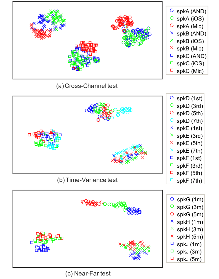
Figure 1: The distributions of x-vectors in three test scenarios. Each shape represents one speaker and each color represents a condition, which is (a) device in the Cross-Channel test, (b) recording session in the Time-Variance test, and (c) recording distance in the Near-Far test.

We further will evaluate some statistical quantities for data in different conditions and analyze the differences on the quantities from one condition to another. The tested quantities are explained as follows:

• Between-speaker and within-speaker variances. Since the covariance matrices (either between-speaker or within-speaker) of different conditions may be in different directions, we test the variance in the principle directions of each condition. Specifically, we select one condition and estimate an LDA transformation, and then project x-vectors of the test speech in all the conditions (including the enrollment condition itself) to the LDA space. Finally, we plot the between-speaker and within-speaker variances on dimensions that correspond to the $50$ leading directions of the LDA transformation.

• Angle metric and length metric to measure the global shift. The global mean vectors of x-vectors in the enrollment condition $\boldsymbol{x}_{e}$ and the test condition $\boldsymbol{x}_{t}$ are firstly computed, and then the cosine distance and Euclidean distance between them are computed as the angle metric and length metric to measure the global shift. The angle metric is formulated by:

  $$\theta=(1-\frac{\boldsymbol{x}_{e}^{T}\boldsymbol{x}_{t}}{||\boldsymbol{x}_{e}||~{}||\boldsymbol{x}_{t}||})*10^{3},$$ (22)

  and the length metric is formulated by:

  $$\ell=||\boldsymbol{x}_{e}-\boldsymbol{x}_{t}||^{2}*10^{2}.$$ (23)

V-C1 Cross-Channel test

We use AIShell-1.Train to compute the statistics. The dataset involves $340$ speakers recorded with $3$ recording devices at the same time.

The between-speaker and within-speaker variances of the test data are reported in Figure 2, where each enrollment condition is presented separately. The observations are: (1) The pattern of the between-speaker variances are not significantly different for different enrollment conditions, and for each enrollment condition, the between-speaker variances for test in different conditions are also similar. (2) For each of the enrollment condition, the pattern of within-speaker variances is different for test in different conditions, but the difference is rather marginal. The within-class variances under enrollment-test mismatched conditions are in the range of $0.8$ to $1.2$, which is close to $1.0$ that is the optimal value under enrollment-test matched conditions (e.g., Mic-Mic).

The angle metric and length metric that measure the global shift are reported in Table I, where we report the results with all pairs of mismatched conditions. Note that for global shift, the mismatch is symmetric for enrollment and test. It can be observed that the global shift is evident in all the mismatched conditions, and the shift between AND and iOS is much smaller than that between Mic and AND/iOS.

All the results coincide the observations in the qualitative analysis, and suggest that in the Cross-Channel test, the enrollment-test mismatch is mainly reflected in a global shift. Therefore, it can be compensated for by a simple shifting back, as formulated by the first special case of the SD/LT approach.

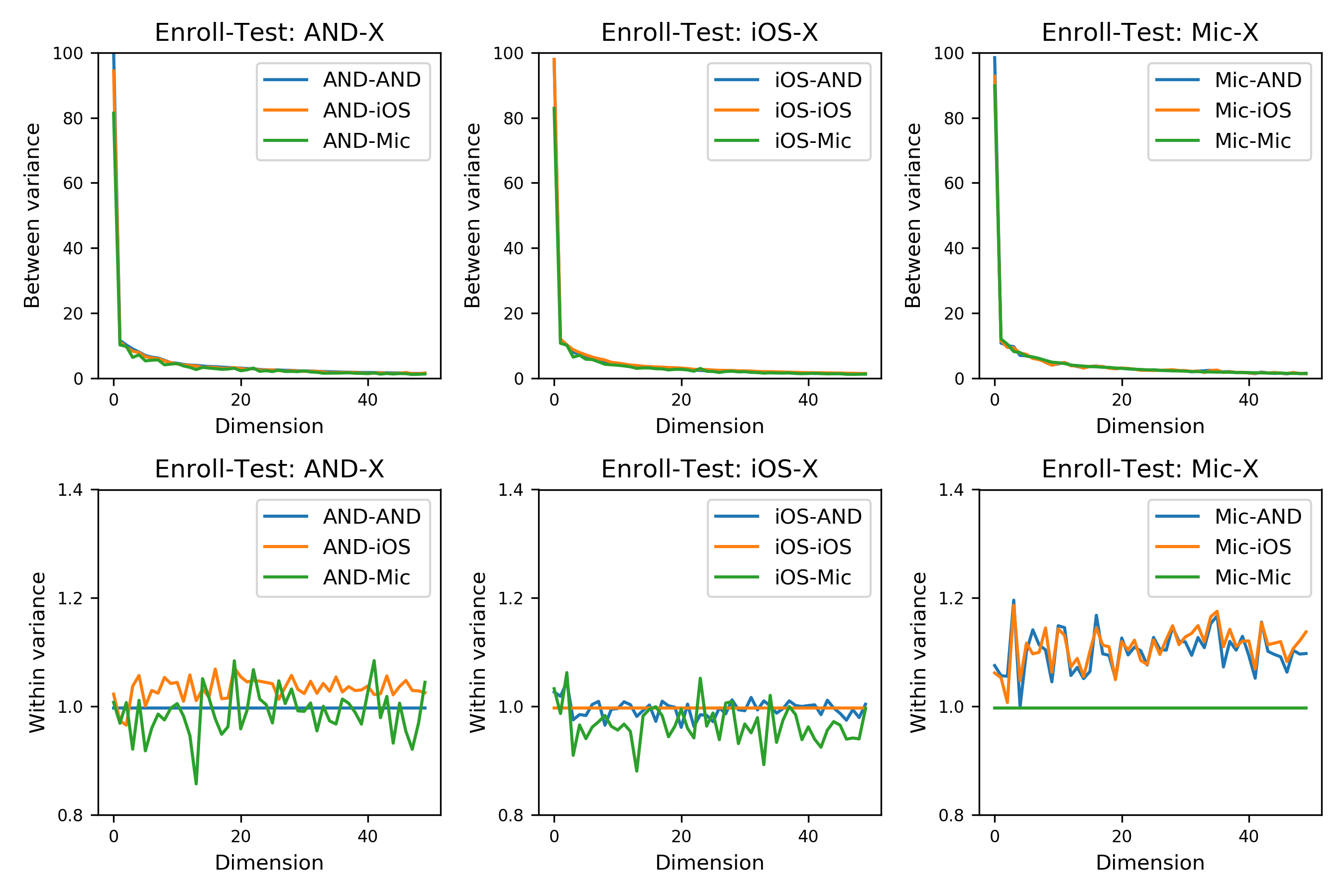
Figure 2: Between-speaker and within-speaker variances (the first $50$ dimensions) in the Cross-Channel test.

TABLE I: Angle metric and length metric in the Cross-Channel test.

Enroll-Test	Angle ($\theta$)	Length ($\ell$)
AND-iOS	0.940	4.673
iOS-Mic	5.199	10.789
Mic-AND	5.645	10.867

V-C2 Time-Variance test

We use the CSLT-Chronos dataset to measure the statistics incoherence in the Time-Variance test. The dataset involves $57$ speakers recorded with $8$ recording sessions in the same acoustic environment. The data of the first session is used for enrollment, and all the $8$ sessions are used for test. In order to study the incremental change on the statistics, we perform a serial test where the test sessions are gradually added to the test data. For example, the test 1st-[1st:5th] means the enrollment is based on the first session, and the test is based on the data from the first to the fifth sessions. Note that the test 1st-[1st:1st] is the condition-matched test.

The between-speaker and within-speaker variances of the test data are reported in Figure 3, where the enrollment is based on the first session in all the test cases. It can be observed that with more sessions involved in the test data, the pattern of the between-speaker variances does not change much, but the within-speaker variances are gradually increased and finally converge to stable values. The angle metric and length metric for the condition-mismatched tests are reported in Table II. Compared to the values in the Cross-Channel test shown in Table I, one can find that the global shift is much smaller in the Time-Variance test.

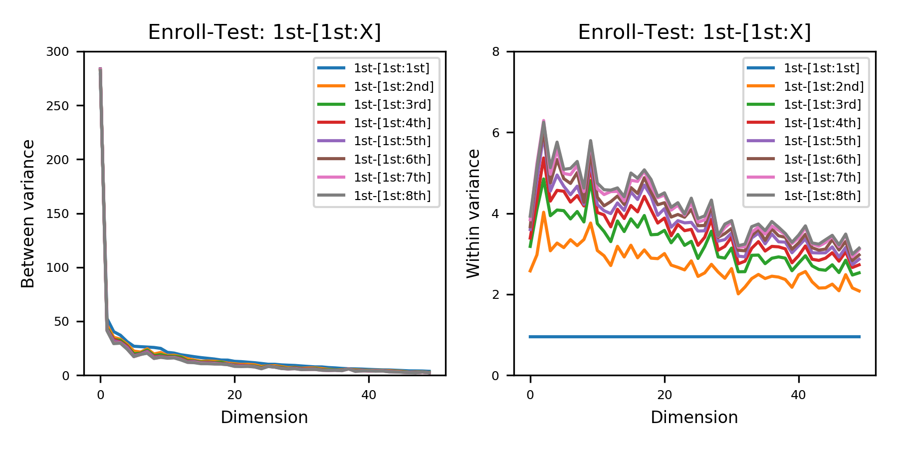
Figure 3: Between-speaker and within-speaker variances (the first $50$ dimensions) in the Time-Variance test.

TABLE II: Angle metric and length metric for global shift in the Time-Variance test.

Enroll-Test	Angle ($\theta$)	Length ($\ell$)
1st-[1st:2nd]	0.085	1.615
1st-[1st:3rd]	0.159	2.326
1st-[1st:4th]	0.234	2.654
1st-[1st:5th]	0.269	2.991
1st-[1st:6th]	0.301	3.224
1st-[1st:7th]	0.346	3.439
1st-[1st:8th]	0.393	3.590

All these observations are consistent with the results obtained from the qualitative analysis presented in the previous section. From these observations, we can conclude that in the Time-Variance test, the enrollment-test mismatch mainly impacts the within-speaker variance. Therefore, a simple within-speaker variance adaptation may be a good approach to alleviate the mismatch, as assumed by the second special case of the SD/LT approach.

V-C3 Near-Far test

The HI-MIA.Train dataset is used to compute the statistics in the Near-Far test. It involves $254$ speakers recorded with $3$ recording distances at the same time.

Similar to in the Cross-Channel test, we examine the between-speaker and within-speaker variances of the test data and present them independently on three enrollment conditions. The results are shown in Figure 4. Firstly, it can be observed that the patterns of the between-speaker variances with the three enrollment conditions are different: enrolling with the near-filed data ($1$m) shows a relatively large between-speaker variance. Moreover, in each enrollment condition, the near-field test data shows a higher between-speaker variance. These observations demonstrated that: (1) the near-field data is more speaker discriminative on either the enrollment or test condition; (2) the mismatch between the near-field and far-field data is reflected in the between-speaker variance.

Paying attention to the within-speaker variance, it shows that in all the enrollment conditions, the condition-matched test data (e.g., $3$m-$3$m) show the smallest and theoretically correct within-speaker variance; all the condition-mismatched test data exhibit larger within-speaker variances. It suggests that the within-speaker variances in different conditions are different.

The angle metric and length metric are reported in Table III. It can be observed that the global shifts between two different conditions are significant, when compared to the results in Cross-Channel test (Table I) and Time-Variance test (Table II). Moreover, the global shift between the two far-field conditions is much smaller than that between the near-field condition and the two far-field conditions.

As a summary, in the Near-Far test, the statistics incoherence is highly complex. It involves mismatch in both the between-speaker and within-speaker variances, as well as a clear global shift. Therefore, it cannot be well addressed by the two special cases of the SD/LT approach; the general form of SD/LT should be employed.

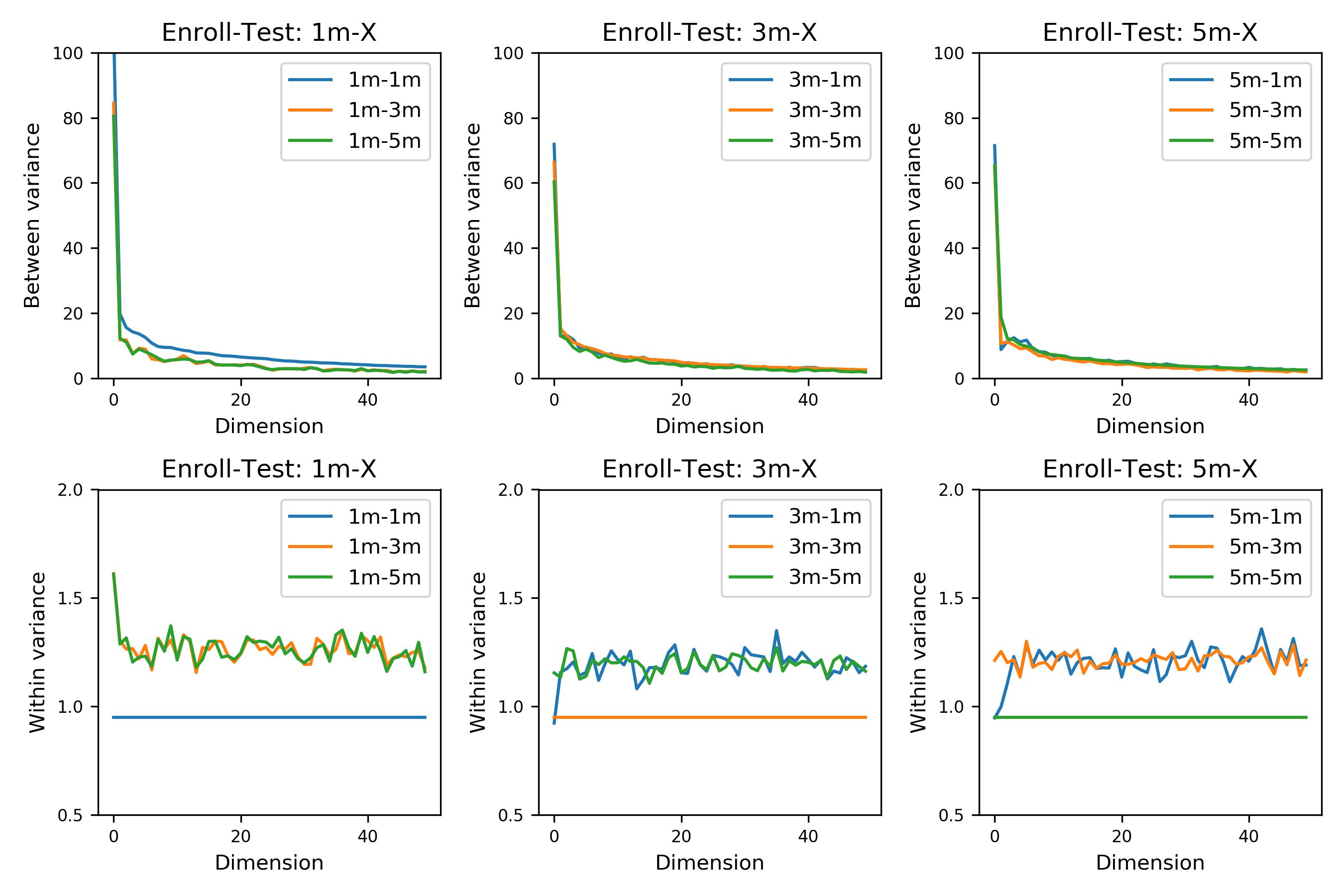
Figure 4: Between-speaker and within-speaker variances (the first 50 dimensions) in the Near-Far test.

TABLE III: Angle metric and length metric in the Near-Far test.

Enroll-Test	Angle ($\theta$)	Length ($\ell$)
1m-3m	4.959	10.745
1m-5m	6.509	11.890
3m-5m	1.703	4.319

V-D Scoring methods in comparison

We verify the SD/LT method on the speaker recognition task, by comparing different forms of SD/LT (two special cases and one general form) and several baseline methods. To make the comparison fair, we categorize these methods by the data it requires: the no-data methods do not require any data from the test condition; the unparallel-data methods require data from the test condition but the data are independent from the enrollment data; the parallel-data methods require data from the test condition and the speakers are shared with the enrollment data.

All the methods are based on the PLDA scoring, with the PLDA models [45] implemented using the Kaldi toolkit [75]. The SD/LT source code has been published online.

V-D1 Non-data methods

• Baseline: The basic PLDA scoring approach where the statistical models are trained with development set in the enrollment condition, and the model is employed to perform the test by ignoring the enrollment-test mismatch.

V-D2 Nonparallel-data methods

• IDVC: Inter-dataset variability compensation (IDVC). It is a popular unsupervised domain normalization technique [37], and has shown great advantage especially in cross-channel scenarios [39]. In our experiments, IDVC is implemented using the nuisance attribute projection (NAP) method [77]. We combine the development data from both enrollment and test conditions to estimate the IDVC projection. For each of the two conditions, the data is split to $n$ subsets and the center vectors of all the subsets are computed. NAP is then performed with the 2$n$ center vectors ($n$ from enroll and $n$ from test). We experimented various configurations and found the optimal $n$ is 2, 20, 5 for the cross-channel test, time-variance test and near-far test, respectively. The optimal $n$ is used in the evaluation.

• GSC: Global shift compensation (GSC). It corresponds to the special case 1 of the SD/LT approach, as mentioned in Section III-B, and assumes that the enrollment-test mismatch can be largely compensated for by a global shift, as shown in Eq.(20). Note that the global shift can be easily computed by the nonparallel development data. Due to the previous qualitative and quantitative analysis, we expect that this method is effective in the Cross-Channel test.

• WVA: Within variance adaptation (WVA). It corresponds to the special case 2 of the SD/LT approach, as mentioned in Section III-C. It assumes that the enrollment-test mismatch is mainly due to the difference in the within-speaker variance, and so can be compensated for by using the correct within-speaker variance as Eq. (21). Note that the within-speaker variances in the enrollment and test conditions can be obtained using the nonparallel development data. Due to the previous qualitative and quantitative analysis, we expect this method is effective in the Time-Variance test.

V-D3 Parallel-data methods

• SD/LT: Statistics decomposition with linear transformation (SD/LT). It corresponds to the general form as mentioned in Section III-A. This model is a linear transformation $\boldsymbol{x}=\mathbf{M}\hat{\boldsymbol{x}}+\boldsymbol{b}$ that maps the test sample $\hat{\boldsymbol{x}}$ to the enrollment condition so that $\hat{\boldsymbol{x}}$ can be represented by the statistical model of the enrollment condition. Importantly, the transformation is only used to compute the likelihood term $p_{k}(\boldsymbol{x})$; and the normalization term $p(\boldsymbol{x})$ is still computed using the statistical model of the test condition, based on the original test data $\hat{\boldsymbol{x}}$. We implemented it based on the MLE criterion with the training objective shown in Eq. (18). In our experiment, the Adam optimizer [78] was used to optimize the parameters $\{\mathbf{M},\boldsymbol{b}\}$.

• MCT: Multi-condition training (MCT). A widely used baseline approach to deal with enrollment-test condition mismatch. In this method, data from both the enrollment and test conditions are pooled together, and then are used to train the PLDA model. This model can be regarded as an interpolation of the statistical models for the enrollment and test conditions. Although not an optimal solution, MCT often delivers good performance in practice. Note that it requires parallel data to discover the speaker subspace shared by different conditions.

• CAT: Condition-adaptation training (CAT). Another simple baseline that transforms speaker vectors from the test condition to the enrollment condition and then performs the scoring there. The transformation is linear and is the same as in SD/LT, defined by $\boldsymbol{x}=\mathbf{M}\hat{\boldsymbol{x}}+\boldsymbol{b}$, and the parameters $\{\mathbf{M},\boldsymbol{b}\}$ are estimated using the same ML training as the SD/LT approach. We highlight that the main difference between SD/LT and CAT is that for SD/LT, the normalization term $p(\boldsymbol{x})$ of the LLR score is computed using the model of the test condition; while for CAT, it is computed using the model of the enrollment condition. This difference is not trivial: the normalization term computed in the test condition is optimal if the statistical model for the test condition is accurate, so SD/LT will be MBR optimal under that condition, but CAT is not.

V-E Speaker recognition results

In this section, experimental results in terms of equal error rate (EER) are presented for the three speaker recognition tests: the Cross-Channel test, the Time-Variance test and the Near-Far test. We will use ‘Base’, ‘NPD’, ‘PD’ to represent the Baseline method, the nonparallel-data methods (including GSC and WVA), and the parallel-data methods (including SD/LT, MCT and CAT), respectively. We also report the performance with AS-norm applied upon SD/LT scores, to show the potential complementarity of the two approaches. For comparison, the results of the baseline system with AS-norm are also reported.

V-E1 Cross-Channel test

In this test, the statistical models of all the scoring methods are trained with the AIShell-1.Dev dataset, and the results on the AIShell-1.Eval dataset are reported in Table IV. The observations are as follows.

TABLE IV: EER(%) on the Cross-Channel test.

Enroll-Test	Base	Base + AS-norm	NPD			PD
			IDVC	GSC	WVA	MCT	CAT	SD/LT	SD/LT + AS-norm
AND-AND	0.797	0.684	-	-	-	-	-	-	-
AND-Mic	2.146	1.316	1.768	1.764	2.165	1.151	1.245	0.981	0.943
AND-iOS	1.425	0.741	1.354	1.382	1.401	1.161	1.312	0.623	0.760
Mic-AND	2.175	1.382	1.665	1.665	2.033	1.161	1.189	0.712	1.128
Mic-Mic	0.778	0.849	-	-	-	-	-	-	-
Mic-iOS	2.251	1.231	1.920	1.892	2.081	1.293	1.481	0.812	1.038
iOS-AND	1.599	0.972	1.382	1.430	1.590	1.156	1.184	0.755	0.854
iOS-Mic	2.216	1.330	1.726	1.759	2.231	1.137	1.231	1.052	0.948
iOS-iOS	0.920	0.684	-	-	-	-	-	-	-

• The performance with enrollment-test matched conditions is much higher than those with mismatched conditions, which indicates that the enrollment-test mismatch is indeed a serious problem for speaker recognition. Moreover, the performance loss with different mismatched condition pairs is different. For instance, The pair AND-iOS obtains better performance than the pair AND-Mic. This is consistent to the observations in the qualitative and quantitative analysis, in particular the results in Figure 2 and Table I.

• For the nonparallel-data methods, IDVC and GSC consistently outperform the baseline on all these mismatched conditions, while WVA does not show much advantage. This observation supports our argument that the main effect of the cross-channel mismatch is a global shift, and even a simple GSC can compensate for the mismatch to a large extent. Besides, it can be found that IDVC is superior to GSC. This indicates dataset-invariant projection by IDVC works better than simple mean subtraction by GSC.

• The three parallel-data methods deliver much better performance than the two nonparallel-data methods. That is not surprising as the parallel-data methods utilize extra information of cross-channel speakers. Moreover, the proposed SD/LT approach consistently outperforms MCT and CAT, demonstrating that SD/LT is a more effective approach in dealing with enrollment-test mismatch. The comparison between SD/LT and CAT is especially interesting, as the two methods look very similar and only differ in the normalization term. The clear advantage of SD/LT demonstrated the importance of a principle solution based on a solid theory.

• The AS-norm consistently improves the baseline results, confirming its effectiveness. However, when applied together with SD/LT, no consistent improvement is observed. A possible reason is that the SD/LT performance has been sufficiently optimal, leaving little space for the AS-norm to make contribution.

V-E2 Time-variance test

The test is conducted with the CSLT-Chronos dataset, which consists of 57 speakers and each speaker has 150 utterances. The first 20 utterances of each speaker are selected as the enrollment set, as well as the development set to train the scoring methods. The rest 130 utterances are used for evaluation. The EER results are reported in Table V. The observations are as follows.

TABLE V: EER(%) on the Time-Variance test.

Enroll-Test	Base	Base + AS-norm	NPD			PD
			IDVC	GSC	WVA	MCT	CAT	SD/LT	SD/LT + AS-norm
1st-[1st:1st]	4.799	5.016	-	-	-	-	-	-	-
1st-[1st:2nd]	6.400	6.306	6.258	6.346	5.934	5.258	5.549	4.339	5.218
1st-[1st:3rd]	6.863	6.282	6.669	6.777	6.156	4.976	5.233	4.062	5.111
1st-[1st:4th]	6.884	6.256	6.850	6.810	6.084	4.619	4.882	3.710	4.612
1st-[1st:5th]	7.108	6.309	6.846	7.022	6.230	4.348	4.804	3.678	4.413
1st-[1st:6th]	7.856	6.832	7.595	7.768	6.938	4.348	4.861	3.661	4.298
1st-[1st:7th]	7.906	7.015	7.618	7.825	7.005	4.262	4.903	3.749	4.473
1st-[1st:8th]	7.881	7.034	7.737	7.815	6.993	4.300	5.041	3.937	4.499

• With more sessions involved in the test data, the performance of the baseline system is gradually reduced, and finally tends to converge to a stable value. This is consistent with our qualitative and quantitative analysis that with more sessions involved, the within-speaker variance will be gradually increased, leading to more severe enrollment-test mismatch.

• Looking at the performance of the three nonparallel-data methods, it can be found that compared with the baseline, WVA obtains obvious performance improvement in all the test conditions, while IDVC/GSC does not show much help. This supports our argument that the main effect of the time-variance mismatch is on the within-speaker variance.

• Again, the three parallel-data methods attain much better performance than the two nonparallel-data methods, and SD/LT attains the best performance. Interestingly, when the test data is sufficiently large, the SD/LT performance is even better than the condition-matched baseline, i.e., the test 1st-[1st:1st]. We attribute this good performance to the more reliable estimation for the within-speaker and between-speaker variances of the test condition. As a comparison, the CAT performance is never better than the condition-matched baseline, as it does not fully use the statistical model of the test condition.

• The AS-norm slightly improves the baseline results for scenarios with enrollment-test mismatch, but impairs the performance for scenarios without such mismatch. The performance loss is also observed in the results applied upon SD/LT. This may be attributed to the limited cohort speakers in the test set (57 speakers in total), which prevents reliable estimation for the score distribution. This imperfect estimation may worsen the performance if the score normalization is not very necessary, e.g., if no enrollment-test mismatch exists, or if the mismatch has been compensated for by SD/LT.

V-E3 Near-Far field test

In this test, the HI-MIA.Dev dataset is used to train the scoring methods, and the results on the HI-MIA.Eval dataset are reported in Table VI. The observations are as follows.

TABLE VI: EER(%) on the Near-Far test.

Enroll-Test	Base	Base + AS-norm	NPD			PD
			IDVC	GSC	WVA	MCT	CAT	SD/LT	SD/LT + AS-norm
1m-1m	0.620	0.465	-	-	-	-	-	-	-
1m-3m	3.968	2.672	3.725	3.725	3.644	2.510	3.563	2.996	2.591
1m-5m	4.866	3.244	4.623	4.623	4.623	3.082	4.623	3.731	2.676
3m-1m	1.938	0.930	1.628	1.705	1.705	1.318	1.628	1.085	0.698
3m-3m	0.891	0.648	-	-	-	-	-	-	-
3m-5m	3.244	2.028	3.244	3.325	3.082	2.595	3.244	2.433	1.703
5m-1m	3.566	1.938	3.333	3.256	3.411	2.326	2.481	2.171	1.395
5m-3m	2.834	1.538	2.753	2.591	2.591	2.105	2.753	2.105	1.619
5m-5m	1.135	1.054	-	-	-	-	-	-	-

• The performance is seriously degraded with the near-far recording mismatch, especially when enroll with near-field data and test on far-field data.

• The three nonparallel-data methods, IDVC, GSC and WVA, all offer reasonable performance improvement compared to the baseline. This is consistent with our quantitative analysis that this recording condition mismatch incurs both incoherence on within-speaker variances and global shift.

• Again, the three parallel-data methods offers more performance gains, as in the Cross-Channel test and the Time-Variance test. A slight difference is that in this test, SD/LT does not always obtain the best performance. Among the 6 mismatched conditions, MCT outperforms SD/LT in two conditions. This is a little surprising as SD/LT is MBR optimal in theory. More careful analysis shows that it is probably because the nature of linear transformation cannot address complex statistics incoherence caused by the near-far recording mismatch.

• Finally, the AS-norm improves both the baseline and the SD/LT results. This is a little different from the observation in the cross-channel/time-variance tests where the AS-norm does not provide consistent improvement upon the SD/LT results. This again may be attributed to the suboptimal SD/LT results due to the linear transformation.

VI Conclusions

This paper investigated the issue of enrollment-test mismatch in speaker recognition, and presented a statistics decomposition (SD) approach to solve this problem. Specifically, we decouple the scoring process to three separated phases according to the decomposed formulation of the PLDA scoring, and statistics from different conditions are used in different phases. This SD approach guarantees that the resultant scores are MBR optimal, and therefore is a principle solution for the enrollment-test mismatch problem.

As an initial study, we proposed an implementation of the SD approach based on a linear transformation (SD/LT). A comprehensive study was conducted and the experimental results demonstrated that: (1) Different types of mismatch exhibits different statistics incoherence, and so should be treated differently; (2) If the statistics incoherence shows a simple form, a simplified version of SD/LT would be effective. An advantage of these simplified methods is that they only require nonparallel data, i.e., data without cross-condition speakers; (3) If parallel data are available, the general form of SD/LT is highly effective and obtains the best performance among all the competitive methods.

Future work will investigate the conditional transformation based on more complex transformation functions, e.g., a deep neural net. This may significantly improve the performance in scenarios with complex condition mismatch, for instance the near-far recording mismatch in our experiment. Experiments on diverse enrollment-test scenarios will be also conducted to demonstrate the strength of the proposed approach, e.g., in the cross-lingual scenario.

References

- [1] J. P. Campbell, “Speaker recognition: A tutorial,” Proceedings of the IEEE, vol. 85, no. 9, pp. 1437–1462, 1997.
- [2] D. A. Reynolds, “An overview of automatic speaker recognition technology,” in IEEE International Conference on Acoustics, Speech and Signal Processing (ICASSP), vol. 4. IEEE, 2002, pp. IV–4072.
- [3] J. H. Hansen and T. Hasan, “Speaker recognition by machines and humans: A tutorial review,” IEEE Signal processing magazine, vol. 32, no. 6, pp. 74–99, 2015.
- [4] D. A. Reynolds, T. F. Quatieri, and R. B. Dunn, “Speaker verification using adapted Gaussian mixture models,” Digital signal processing, vol. 10, no. 1-3, pp. 19–41, 2000.
- [5] P. Kenny, G. Boulianne, P. Ouellet, and P. Dumouchel, “Joint factor analysis versus eigenchannels in speaker recognition,” IEEE Transactions on Audio, Speech, and Language Processing, vol. 15, no. 4, pp. 1435–1447, 2007.
- [6] N. Dehak, P. J. Kenny, R. Dehak, P. Dumouchel, and P. Ouellet, “Front-end factor analysis for speaker verification,” IEEE Transactions on Audio, Speech, and Language Processing, vol. 19, no. 4, pp. 788–798, 2011.
- [7] L. Deng and D. Yu, “Deep learning: methods and applications,” Foundations and trends in signal processing, vol. 7, no. 3–4, pp. 197–387, 2014.
- [8] E. Variani, X. Lei, E. McDermott, I. L. Moreno, and J. Gonzalez-Dominguez, “Deep neural networks for small footprint text-dependent speaker verification,” in IEEE International Conference on Acoustics, Speech and Signal Processing (ICASSP). IEEE, 2014, pp. 4052–4056.
- [9] L. Li, Y. Chen, Y. Shi, Z. Tang, and D. Wang, “Deep speaker feature learning for text-independent speaker verification,” in Proceedings of the Annual Conference of International Speech Communication Association (INTERSPEECH), 2017, pp. 1542–1546.
- [10] D. Snyder, D. Garcia-Romero, G. Sell, D. Povey, and S. Khudanpur, “X-vectors: Robust DNN embeddings for speaker recognition,” in IEEE International Conference on Acoustics, Speech and Signal Processing (ICASSP). IEEE, 2018, pp. 5329–5333.
- [11] K. Okabe, T. Koshinaka, and K. Shinoda, “Attentive statistics pooling for deep speaker embedding,” in Proceedings of the Annual Conference of International Speech Communication Association (INTERSPEECH), 2018, pp. 2252–2256.
- [12] G. Heigold, I. Moreno, S. Bengio, and N. Shazeer, “End-to-end text-dependent speaker verification,” in IEEE International Conference on Acoustics, Speech and Signal Processing (ICASSP). IEEE, 2016, pp. 5115–5119.
- [13] S.-X. Zhang, Z. Chen, Y. Zhao, J. Li, and Y. Gong, “End-to-end attention based text-dependent speaker verification,” in Spoken Language Technology Workshop (SLT). IEEE, 2016, pp. 171–178.
- [14] F. R. Rahman Chowdhury, Q. Wang, I. L. Moreno, and L. Wan, “Attention-based models for text-dependent speaker verification,” in IEEE International Conference on Acoustics, Speech and Signal Processing (ICASSP), 2018, pp. 5359–5363.
- [15] D. Wang, L. Li, Z. Tang, and T. F. Zheng, “Deep speaker verification: Do we need end to end?” in 2017 Asia-Pacific Signal and Information Processing Association Annual Summit and Conference (APSIPA ASC). IEEE, 2017, pp. 177–181.
- [16] J. S. Chung, A. Nagrani, and A. Zisserman, “VoxCeleb2: Deep speaker recognition,” in Proceedings of the Annual Conference of International Speech Communication Association (INTERSPEECH), 2018, pp. 1086–1090.
- [17] J. weon Jung, H.-S. Heo, J. ho Kim, H. jin Shim, and H.-J. Yu, “RawNet: Advanced end-to-end deep neural network using raw waveforms for text-independent speaker verification,” in Proceedings of the Annual Conference of International Speech Communication Association (INTERSPEECH), 2019, pp. 1268–1272.
- [18] W. Cai, J. Chen, and M. Li, “Exploring the encoding layer and loss function in end-to-end speaker and language recognition system,” in Proceedings of Odyssey: The Speaker and Language Recognition Workshop, 2018, pp. 74–81.
- [19] W. Xie, A. Nagrani, J. S. Chung, and A. Zisserman, “Utterance-level aggregation for speaker recognition in the wild,” in IEEE International Conference on Acoustics, Speech and Signal Processing (ICASSP), 2019, pp. 5791–579.
- [20] N. Chen, J. Villalba, and N. Dehak, “Tied mixture of factor analyzers layer to combine frame level representations in neural speaker embeddings,” in Proceedings of the Annual Conference of International Speech Communication Association (INTERSPEECH), 2019, pp. 2948–2952.
- [21] L. Li, D. Wang, C. Xing, and T. F. Zheng, “Max-margin metric learning for speaker recognition,” in 10th International Symposium on Chinese Spoken Language Processing (ISCSLP), 2016, pp. 1–4.
- [22] W. Ding and L. He, “MTGAN: Speaker verification through multitasking triplet generative adversarial networks,” in Proceedings of the Annual Conference of International Speech Communication Association (INTERSPEECH), 2018, pp. 3633–3637.
- [23] J. Wang, K.-C. Wang, M. T. Law, F. Rudzicz, and M. Brudno, “Centroid-based deep metric learning for speaker recognition,” in IEEE International Conference on Acoustics, Speech and Signal Processing (ICASSP). IEEE, 2019, pp. 3652–3656.
- [24] Z. Bai, X.-L. Zhang, and J. Chen, “Partial AUC optimization based deep speaker embeddings with class-center learning for text-independent speaker verification,” in IEEE International Conference on Acoustics, Speech and Signal Processing (ICASSP). IEEE, 2020, pp. 6819–6823.
- [25] Z. Gao, Y. Song, I. McLoughlin, P. Li, Y. Jiang, and L.-R. Dai, “Improving aggregation and loss function for better embedding learning in end-to-end speaker verification system,” in Proceedings of the Annual Conference of International Speech Communication Association (INTERSPEECH), 2019, pp. 361–365.
- [26] J. Zhou, T. Jiang, Z. Li, L. Li, and Q. Hong, “Deep speaker embedding extraction with channel-wise feature responses and additive supervision softmax loss function,” in Proceedings of the Annual Conference of International Speech Communication Association (INTERSPEECH), 2019, pp. 2883–2887.
- [27] R. Li, N. Li, D. Tuo, M. Yu, D. Su, and D. Yu, “Boundary discriminative large margin cosine loss for text-independent speaker verification,” in IEEE International Conference on Acoustics, Speech and Signal Processing (ICASSP). IEEE, 2019, pp. 6321–6325.
- [28] S. Wang, J. Rohdin, L. Burget, O. Plchot, Y. Qian, K. Yu, and J. Cernocky, “On the usage of phonetic information for text-independent speaker embedding extraction,” in Proceedings of the Annual Conference of International Speech Communication Association (INTERSPEECH), 2019, pp. 1148–1152.
- [29] T. Stafylakis, J. Rohdin, O. Plchot, P. Mizera, and L. Burget, “Self-supervised speaker embeddings,” in Proceedings of the Annual Conference of International Speech Communication Association (INTERSPEECH), 2019, pp. 2863–2867.
- [30] M. McLaren and D. Van Leeuwen, “Source-normalized lda for robust speaker recognition using i-vectors from multiple speech sources,” IEEE Transactions on Audio, Speech, and Language Processing, vol. 20, no. 3, pp. 755–766, 2011.
- [31] S. Shon, S. Mun, W. Kim, and H. Ko, “Autoencoder based domain adaptation for speaker recognition under insufficient channel information,” in Proceedings of the Annual Conference of International Speech Communication Association (INTERSPEECH), 2017, pp. 1014–1018.
- [32] Q. Wang, W. Rao, S. Sun, L. Xie, E. S. Chng, and H. Li, “Unsupervised domain adaptation via domain adversarial training for speaker recognition,” in IEEE International Conference on Acoustics, Speech and Signal Processing (ICASSP), 2018, pp. 4889–4893.
- [33] J. Villalba and E. Lleida, “Bayesian adaptation of PLDA based speaker recognition to domains with scarce development data,” in Proceedings of Odyssey: The Speaker and Language Recognition Workshop, 2012, pp. 47–54.
- [34] D. Garcia-Romero and A. McCree, “Supervised domain adaptation for i-vector based speaker recognition,” in IEEE International Conference on Acoustics, Speech and Signal Processing (ICASSP), 2014, pp. 4047–4051.
- [35] D. Garcia-Romero, A. McCree, S. Shum, and C. Vaquero, “Unsupervised domain adaptation for i-vector speaker recognition,” in Proceedings of Odyssey: The Speaker and Language Recognition Workshop, 2014.
- [36] O. Glembek, J. Ma, P. Matějka, B. Zhang, O. Plchot, L. Bürget, and S. Matsoukas, “Domain adaptation via within-class covariance correction in i-vector based speaker recognition systems,” in IEEE International Conference on Acoustics, Speech and Signal Processing (ICASSP). IEEE, 2014, pp. 4032–4036.
- [37] H. Aronowitz, “Inter dataset variability compensation for speaker recognition,” in IEEE International Conference on Acoustics, Speech and Signal Processing (ICASSP), 2014, pp. 4002–4006.
- [38] H. Aronowitz, “Compensating inter-dataset variability in PLDA hyper-parameters for robust speaker recognition.” in Proceedings of Odyssey: The Speaker and Language Recognition Workshop, 2014, pp. 280–286.
- [39] A. Kanagasundaram, D. Dean, and S. Sridharan, “Improving out-domain PLDA speaker verification using unsupervised inter-dataset variability compensation approach,” in IEEE International Conference on Acoustics, Speech and Signal Processing (ICASSP), 2015, pp. 4654–4658.
- [40] M. H. Rahman, A. Kanagasundaram, I. Himawan, D. Dean, and S. Sridharan, “Improving PLDA speaker verification performance using domain mismatch compensation techniques,” Computer Speech & Language, vol. 47, pp. 240–258, 2018.
- [41] E. Shriberg, M. Graciarena, H. Bratt, A. Kathol, S. S. Kajarekar, H. Jameel, C. Richey, and F. Goodman, “Effects of vocal effort and speaking style on text-independent speaker verification,” in Proceedings of the Annual Conference of International Speech Communication Association (INTERSPEECH), 2008.
- [42] C. Zhang, S. Ranjan, and J. H. Hansen, “An analysis of transfer learning for domain mismatched text-independent speaker verification,” in Proceedings of Odyssey: The Speaker and Language Recognition Workshop, 2018, pp. 181–186.
- [43] S. J. Park, C. Sigouin, J. Kreiman, P. A. Keating, J. Guo, G. Yeung, F.-Y. Kuo, and A. Alwan, “Speaker identity and voice quality: Modeling human responses and automatic speaker recognition.” in Proceedings of the Annual Conference of International Speech Communication Association (INTERSPEECH), 2016, pp. 1044–1048.
- [44] A. Afshan, J. Guo, S. J. Park, V. Ravi, A. McCree, and A. Alwan, “Variable frame rate-based data augmentation to handle speaking-style variability for automatic speaker verification,” arXiv preprint arXiv:2008.03616, 2020.
- [45] S. Ioffe, “Probabilistic linear discriminant analysis,” in European Conference on Computer Vision (ECCV). Springer, 2006, pp. 531–542.
- [46] S. J. Prince and J. H. Elder, “Probabilistic linear discriminant analysis for inferences about identity,” in 2007 IEEE 11th International Conference on Computer Vision. IEEE, 2007, pp. 1–8.
- [47] L. Ferrer and M. McLaren, “Joint plda for simultaneous modeling of two factors,” The Journal of Machine Learning Research, vol. 20, no. 1, pp. 847–875, 2019.
- [48] L. Ferrer and M. McLaren, “A generalization of plda for joint modeling of speaker identity and multiple nuisance conditions.” in INTERSPEECH, 2018, pp. 82–86.
- [49] N. Brümmer and J. Du Preez, “Application-independent evaluation of speaker detection,” Computer Speech & Language, vol. 20, no. 2-3, pp. 230–275, 2006.
- [50] M. McLaren, A. Lawson, L. Ferrer, N. Scheffer, and Y. Lei, “Trial-based calibration for speaker recognition in unseen conditions,” in Proc. Odyssey, 2014, pp. 19–25.
- [51] M. I. Mandasari, R. Saeidi, M. McLaren, and D. A. van Leeuwen, “Quality measure functions for calibration of speaker recognition systems in various duration conditions,” IEEE Transactions on Audio, Speech, and Language Processing, vol. 21, no. 11, pp. 2425–2438, 2013.
- [52] N. Brümmer and E. De Villiers, “The speaker partitioning problem.” in Odyssey, 2010, p. 34.
- [53] A. Sizov, K. A. Lee, and T. Kinnunen, “Unifying probabilistic linear discriminant analysis variants in biometric authentication,” in Joint IAPR International Workshops on Statistical Techniques in Pattern Recognition (SPR) and Structural and Syntactic Pattern Recognition (SSPR). Springer, 2014, pp. 464–475.
- [54] P. Kenny, T. Stafylakis, P. Ouellet, M. J. Alam, and P. Dumouchel, “PLDA for speaker verification with utterances of arbitrary duration,” in IEEE International Conference on Acoustics, Speech and Signal Processing (ICASSP). IEEE, 2013, pp. 7649–7653.
- [55] B. J. Borgström and A. McCree, “Discriminatively trained bayesian speaker comparison of i-vectors,” in IEEE International Conference on Acoustics, Speech and Signal Processing (ICASSP). IEEE, 2013, pp. 7659–7662.
- [56] A. McCree, G. Sell, and D. Garcia-Romero, “Extended variability modeling and unsupervised adaptation for plda speaker recognition.” in Proceedings of the Annual Conference of International Speech Communication Association (INTERSPEECH), 2017, pp. 1552–1556.
- [57] D. Wang, “Remarks on optimal scores for speaker recognition,” CSLT@Tsinghua University, 2020. [Online]. Available: http://wangd.cslt.org/public/pdf/nl.pdf
- [58] D. Wang, “A simulation study on optimal scores for speaker recognition,” EURASIP Journal on Audio, Speech, and Music Processing, vol. 2020, no. 1, pp. 1–23, 2020.
- [59] I. J. Myung, “Tutorial on maximum likelihood estimation,” Journal of mathematical Psychology, vol. 47, no. 1, pp. 90–100, 2003.
- [60] C. J. Leggetter and P. C. Woodland, “Maximum likelihood linear regression for speaker adaptation of continuous density hidden Markov models,” Computer speech & language, vol. 9, no. 2, pp. 171–185, 1995.
- [61] J. Williams and S. King, “Disentangling style factors from speaker representations,” in Proceedings of the Annual Conference of International Speech Communication Association (INTERSPEECH), 2019, pp. 3945–3949.
- [62] G. Bhattacharya, J. Alam, and P. Kenny, “Adapting end-to-end neural speaker verification to new languages and recording conditions with adversarial training,” in IEEE International Conference on Acoustics, Speech and Signal Processing (ICASSP). IEEE, 2019, pp. 6041–6045.
- [63] W. H. Kang, S. H. Mun, M. H. Han, and N. S. Kim, “Disentangled speaker and nuisance attribute embedding for robust speaker verification,” IEEE Access, 2020.
- [64] K. A. Lee, Q. Wang, and T. Koshinaka, “The CORAL+ algorithm for unsupervised domain adaptation of plda,” in IEEE International Conference on Acoustics, Speech and Signal Processing (ICASSP). IEEE, 2019, pp. 5821–5825.
- [65] Y. Lei, L. Burget, L. Ferrer, M. Graciarena, and N. Scheffer, “Towards noise-robust speaker recognition using probabilistic linear discriminant analysis,” in 2012 IEEE international conference on acoustics, speech and signal processing (ICASSP). IEEE, 2012, pp. 4253–4256.
- [66] P. Rajan, T. Kinnunen, and V. Hautamäki, “Effect of multicondition training on i-vector plda configurations for speaker recognition.” in Interspeech. Citeseer, 2013, pp. 3694–3697.
- [67] P. Matejka, O. Novotnỳ, O. Plchot, L. Burget, M. D. Sánchez, and J. Cernockỳ, “Analysis of score normalization in multilingual speaker recognition.” in INTERSPEECH, 2017, pp. 1567–1571.
- [68] A. Nagrani, J. S. Chung, and A. Zisserman, “VoxCeleb: a large-scale speaker identification dataset,” arXiv preprint arXiv:1706.08612, 2017.
- [69] H. Bu, J. Du, X. Na, B. Wu, and H. Zheng, “Aishell-1: An open-source mandarin speech corpus and a speech recognition baseline,” in Conference of the Oriental Chapter of the International Coordinating Committee on Speech Databases and Speech I/O Systems and Assessment (O-COCOSDA). IEEE, 2017, pp. 1–5.
- [70] L. Wang and T. F. Zheng, “Creation of time-varying voiceprint database,” in Conference of the Oriental Chapter of the International Coordinating Committee on Speech Databases and Speech I/O Systems and Assessment (O-COCOSDA). IEEE, 2010, pp. 1–5.
- [71] X. Qin, H. Bu, and M. Li, “HI-MIA: A far-field text-dependent speaker verification database and the baselines,” 2019.
- [72] D. Snyder, G. Chen, and D. Povey, “Musan: A music, speech, and noise corpus,” arXiv preprint arXiv:1510.08484, 2015.
- [73] T. Ko, V. Peddinti, D. Povey, M. L. Seltzer, and S. Khudanpur, “A study on data augmentation of reverberant speech for robust speech recognition,” in IEEE International Conference on Acoustics, Speech and Signal Processing (ICASSP). IEEE, 2017, pp. 5220–5224.
- [74] L. Wang, J. Wang, L. Li, T. F. Zheng, and F. K. Soong, “Improving speaker verification performance against long-term speaker variability,” Speech Communication, vol. 79, pp. 14–29, 2016.
- [75] D. Povey, A. Ghoshal, G. Boulianne, L. Burget, O. Glembek, N. Goel, M. Hannemann, P. Motlicek, Y. Qian, P. Schwarz et al., “The Kaldi speech recognition toolkit,” in IEEE 2011 workshop on automatic speech recognition and understanding, no. EPFL-CONF-192584. IEEE Signal Processing Society, 2011.
- [76] L. v. d. Maaten and G. Hinton, “Visualizing data using t-SNE,” Journal of Machine Learning Research, vol. 9, no. Nov, pp. 2579–2605, 2008.
- [77] A. Solomonoff, W. M. Campbell, and C. Quillen, “Nuisance attribute projection,” Speech Communication, pp. 1–73, 2007.
- [78] D. P. Kingma and J. Ba, “Adam: A method for stochastic optimization,” arXiv preprint arXiv:1412.6980, 2014.