Discovery of the Relativistic Schrödinger equation

Abstract.

We discuss the discovery of the relativistic wave equation for a spin-zero charged particle in the Coulomb field by Erwin Schrödinger (and elaborate on why he didn’t publish it).

Wir beleuchten die Entdeckung der relativistischen Wellengleichung für ein geladenes Spin-Null-Teilchen im Coulomb-Feld durch Erwin Schrödinger (und erarbeiten, warum er diese Gleichung nicht veröffentlicht hat).

1. Introduction

There are many great reminiscences and reviews of remarkable events of the early days of quantum mechanics. Among those are [2], [4], [14], [17], [18], [26], [30], [36], [37], [38], [39], [41], [42], [46], [56], [60], [61] (and references therein), as well as great biographies of the ‘pioneers’ of the quantum revolution, namely, Werner Heisenberg [6], [7], Erwin Schrödinger [25], [43], and Paul Dirac [19].

A traditional story of the discovery of Schrödinger’s wave equation – “rumor has it”– goes this way [2], [25], [43]: In early November 1925, Peter Debye, at the ETH, asked Schrödinger to prepare a talk for the Zürich physicists about de Broglie’s work just published in Annales de Physique. The date on which this particular colloquium took place has not been recorded, but it must have been in late November or early December, before the end of the academic term [25], [39]. According to Felix Bloch [2], at the end of Schrödinger’s talk, Debye casually remarked that (de Broglie’s) way of talking was rather childish and someone had to think about an equation for these (de Broglie’s) ‘matter waves’. As a student of Sommerfeld, Debye had learned that to deal properly with waves, one had to have a wave equation. Indeed, at his second talk, just a few weeks later, Schrödinger mentioned: “My colleague Debye suggested that one should have a wave equation; well, I have found one!”

For a sequence of those remarkable events, a direct quote is quite appropriate [25]: “Schrödinger’s first thought was to attempt to find a wave equation, moving on from de Broglie’s work, that would describe the behavior of an electron in the simplest atom, hydrogen. He naturally included in his calculations allowance for the effects described by the special theory of relativity, deriving, probably early in December 1925, what became known as the relativistic Schrödinger (not hydrogen—our correction!) equation. Unfortunately, it didn’t work. The predictions of the relativistic equation did not match up with observations of real atoms. We now know that this is because Schrödinger did not allow for the quantum spin of the electron, which is hardly surprising, since the idea of spin had not been introduced into quantum mechanics at that time. But it is particularly worth taking note of this false start, since it highlights the deep and muddy waters in which quantum physicists go swimming—for you need to take account of spin, a property usually associated with particles, in order to derive a wave equation for the electron!

With the Christmas break coming up, he had an opportunity to get away from Zürich and think things over in the clean air of Arosa … [25] .”(See also [39] and [43] for more details.)

Whereas the honorable historians of science are arguing about the sequence and details of some events [26], [30], [39], [61], our remarks are dedicated to a somewhat missing, modern mathematical, part of this story, namely, the discovery of a relativistic (spin-zero) wave equation by Erwin Schrödinger (and why he did report and publish only the centennial nonrelativistic version for the hydrogen atom).

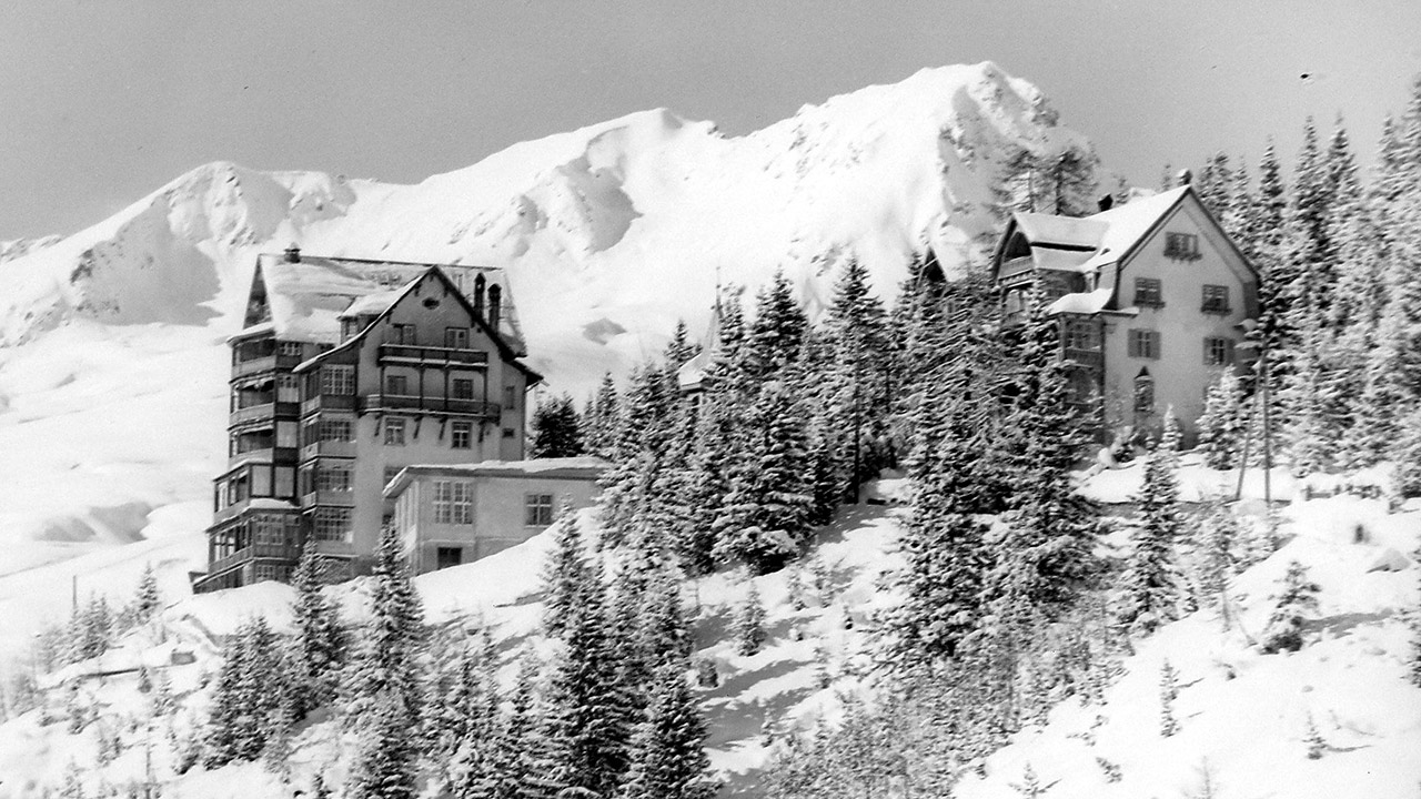
Figure 1. The Villa Herwig–Frisia (right), Arosa, where it is believed wave mechanics was discovered during the Christmas holidays 1925–26.

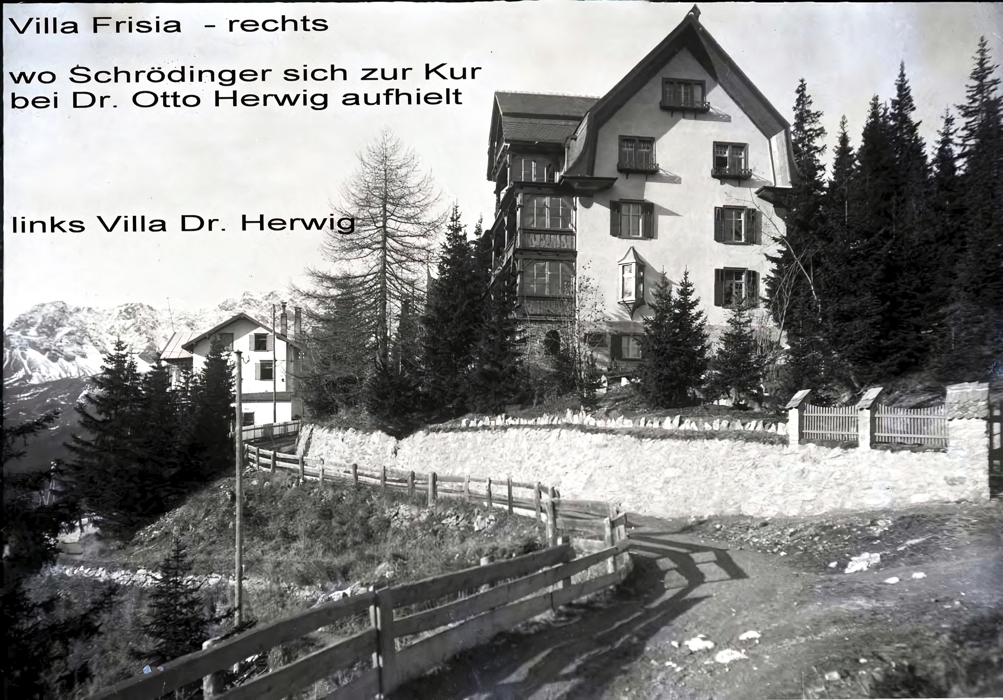
Figure 2. The Villa Herwig–Frisia postcard.

2. Introducing the relativistic Schrödinger equation

How Schrödinger derived his celebrated equation and subsequently applied it to the hydrogen atom? According to his own testimony [49], [54], de Broglie’s seminal work on a wave theory of matter of 1923–24 and Einstein’s work on ideal Bose gases of 1924–25 laid the ground for the discovery of wave mechanics. The crucial phase is dated approximately from late November 1925 to late January 1926 (see, for instance, [30] and [39]).

Let us start our discussion by following the original Schrödinger’s idea — “rumor has it”! For a classical relativistic particle of charge $e$ in the electromagnetic field, one has to replace

$$E^{2}=c^{2}\mathbf{p}^{2}+m^{2}c^{4}$$ (2.1)

by

$$\left(E-e\varphi\right)^{2}=\left(c\mathbf{p}-e\mathbf{A}\right)^{2}+m^{2}c^{4}.$$ (2.2)

In relativistic quantum mechanics, we replace the four-vector of energy $E$ and linear momentum $\mathbf{p}$ with the following operators

$$E\rightarrow\widehat{E}=i\hbar\frac{\partial}{\partial t},\qquad\mathbf{p}\rightarrow\widehat{\mathbf{p}}=-i\hbar\nabla.$$ (2.3)

As a result, we arrive at the relativistic Schrödinger equation [12], [47]:

$$\left(-\hbar^{2}\frac{\partial^{2}}{\partial t^{2}}-2ie\hbar\varphi\frac{\partial}{\partial t}-ie\hbar\frac{\partial\varphi}{\partial t}+e^{2}\varphi^{2}\right)\psi$$ (2.4)

$$\qquad=\left(-\hbar^{2}c^{2}\Delta+2ic\hbar\mathbf{A}\cdot\nabla+2iec\hbar\,\nabla\cdot\mathbf{A}+e^{2}{\mathbf{A}}^{2}+m^{2}c^{4}\right)\psi\/.$$

In the special case of Coulomb field,

$$e\varphi=-\frac{Ze^{2}}{r},\qquad\mathbf{A}=\mathbf{0},$$ (2.5)

one can separate the time and spatial variables

$$\psi\left(\mathbf{r},t\right)=\chi(\mathbf{r})e^{-i(E\;t)/\hbar}.$$ (2.6)

Finally, the stationary relativistic Schrödinger equation takes the form

$$\left(E+\frac{Ze^{2}}{r}\right)^{2}\chi=\left(-\hbar^{2}c^{2}\Delta+m^{2}c^{4}\right)\chi.$$ (2.7)

(As one can see, it is NOT a traditional eigenvalue problem!) The standard rumor says that Schrödinger invented this equation sometime in late 1925, found the corresponding relativistic energy levels, and derived the fine structure formula, different from Sommerfeld’s one [13]. This is why he had to abandon this equation and to consider a nonrelativistic approximation. Moreover, they say that he had to withdraw the ‘relativistically framed’ article, whose draft never been found, from a journal and start all over with his centennial article on the nonrelativistic Schrödinger equation [49]. Our goal here is to follow the original ‘relativistic idea’. Our analysis, nonetheless, will suggest that it is hardly possible to believe that a complete relativistic solution (for a charged spin-zero particle) had been found at that time (see, nonetheless, [39] for an opposite opinion and a remarkable article of Vladimir A. Fock [20] for the first published solution of this problem among other things; see also [21]).

3. Solving the relativistic Schrödinger equation

We follow [44] with somewhat different details (see also [11], [20], [47] for a different approach) and, first of all, separate the variables in spherical coordinates, $\chi\left(r,\theta,\varphi\right)=R(r)Y_{lm}(\theta,\varphi),$ where $Y_{lm}(\theta,\varphi)$ are the spherical harmonics with familiar properties [59]. As a result,

$$\frac{1}{r^{2}}\frac{d}{dr}\left(r^{2}\frac{dR}{dr}\right)+\left[\frac{\left(E+Ze^{2}/r\right)^{2}-m^{2}c^{4}}{\hbar^{2}c^{2}}-\frac{l\left(l+1\right)}{r^{2}}\right]R=0\qquad(l=0,1,2,\;...)$$ (3.1)

Figure 3. A page from Notebook $N1\/$, with the first record of the wave equation [30], [43] (probably written about Christmas 1925).

(see Figure 3 for the original version ). In the dimensionless quantities,

$$\varepsilon=\frac{E}{mc^{2}},\qquad x=\beta r=\frac{mc}{\hbar}r,\qquad\mu=\frac{Ze^{2}}{\hbar c},$$ (3.2)

for the new radial function,

$$R(r)=F(x)=\frac{u(x)}{x},$$ (3.3)

one gets

$$\frac{1}{x^{2}}\frac{d}{dx}\left(x^{2}\frac{dF}{dx}\right)+\left[\left(\varepsilon+\frac{\mu}{x}\right)^{2}-1-\frac{l\left(l+1\right)}{x^{2}}\right]F=0.$$ (3.4)

Given the identity,

$$\frac{1}{x^{2}}\frac{d}{dx}\left(x^{2}\frac{dF}{dx}\right)=\frac{1}{x}\frac{d^{2}}{dx^{2}}\left(xF\right),$$ (3.5)

we finally obtain

$$u^{\prime\prime}+\left[\left(\varepsilon+\frac{\mu}{x}\right)^{2}-1-\frac{l\left(l+1\right)}{x^{2}}\right]u=0.$$ (3.6)

This is the generalized equation of hypergeometric form (A.1) below, when

$$\sigma\left(x\right)=x,\qquad\widetilde{\tau}(x)\equiv 0,\qquad\widetilde{\sigma}(x)=\left(\varepsilon^{2}-1\right)x^{2}+2\mu\varepsilon x+\mu^{2}-l(l+1)$$ (3.7)

(see also Table 2 provided in Appendix A below).

In view of the normalization condition,

$$\int_{0}^{\infty}R^{2}(r)r^{2}\ dr=1,\qquad\text{or\quad}\int_{0}^{\infty}u^{2}(x)\;dx=\beta^{3},\quad\beta=\frac{mc}{\hbar^{2}},$$ (3.8)

it’s useful to start from asymptotic as $r\rightarrow 0$ $($or $x\rightarrow 0).$ In this limit, from (3.6), one gets Euler’s equation:

$$x^{2}u^{\prime\prime}+\left[\mu^{2}-l\left(l+1\right)\right]u=0,$$ (3.9)

which can be solved by the standard substitution $u=x^{\alpha},$ resulting in the following quadratic equation:

$$\alpha^{2}-\alpha+\left[\mu^{2}-l\left(l+1\right)\right]=0.$$ (3.10)

Thus the general solution of Euler’s equation has the form

$$u=C_{1}x^{\nu+1}+C_{2}x^{-\nu};\qquad\nu=-\frac{1}{2}+\sqrt{\left(l+\frac{1}{2}\right)^{2}-\mu^{2}},\quad\mu=\frac{Ze^{2}}{\hbar c};$$ (3.11)

which is bounded as $x\rightarrow 0$ with $C_{2}=0:$ $\ u\simeq C_{1}x^{\nu+1}\/.$

We continue our analysis of Schrödinger’s equation (3.6), applying Nikiforov–Uvarov’s technique, and transform (A.1) into the simpler form (A.3) by using $u\left(x\right)=\varphi\left(x\right)y\left(x\right),$ where

$$\frac{\varphi^{\prime}}{\varphi}=\frac{\pi\left(x\right)}{\sigma\left(x\right)},\qquad\pi(x)=\frac{\sigma^{\prime}-\widetilde{\tau}}{2}\pm\sqrt{\left(\frac{\sigma^{\prime}-\widetilde{\tau}}{2}\right)^{2}-\widetilde{\sigma}+k\sigma},$$ (3.12)

or, in this particular case,

$$\pi(x) = \frac{1}{2}\pm\sqrt{\left(l+\frac{1}{2}\right)^{2}-\mu^{2}-2\mu\varepsilon x+\left(1-\varepsilon^{2}\right)x^{2}+kx}$$ (3.13)

$$= \frac{1}{2}\pm\left\{\begin{array}[]{cc}\sqrt{1-\varepsilon^{2}}\;x+\nu+\frac{1}{2},&k=2\mu\varepsilon+(2\nu+1)\sqrt{1-\varepsilon^{2}};\\ \sqrt{1-\varepsilon^{2}}\;x-\nu-\frac{1}{2},&k=2\mu\varepsilon-(2\nu+1)\sqrt{1-\varepsilon^{2}}.\end{array}\right.$$ (3.16)

Here, one has to choose the second possibility, when $\tau^{\prime}=2\pi^{\prime}<0,$ namely$:$

$$\tau\left(x\right)=2\left(\nu+1-ax\right),\qquad a=\sqrt{1-\varepsilon^{2}}.$$ (3.17)

Thus

$$\pi\left(x\right) = \nu+1-ax,\qquad\qquad\quad\varphi\left(x\right)=x^{\nu+1}e^{-ax};$$ (3.18)

$$\lambda = 2\left(\mu\varepsilon-(\nu+1)a\right),\qquad\rho\left(x\right)=x^{2\nu+1}e^{-2ax}.$$

For example,

$$\left(\ln\varphi\right)^{\prime} = \frac{\nu+1}{x}-a,\qquad\ln\varphi=\left(\nu+1\right)\ln x-ax,\qquad\text{etc.}$$

$$\lambda = k+\pi^{\prime}=2\left(\mu\varepsilon-(\nu+1)a\right).$$

(All these data are collected in Table 2, Appendix A, for the reader’s convenience.)

In Nikiforov–Uvarov’s method, the energy levels can be obtained from the quantization rule [44]:

$$\lambda+n\tau^{\prime}+\frac{1}{2}n\left(n-1\right)\sigma^{\prime\prime}=0\qquad(n=0,1,2,\ ...),$$ (3.19)

which gives Schrödinger’s fine structure formula (for a charged spin-zero particle in the Coulomb field) [20]:

$$E=E_{n_{r}}=\frac{mc^{2}}{\sqrt{1+\left(\dfrac{\mu}{n_{r}+\nu+1}\right)^{2}}}\qquad\left(n=n_{r}=0,1,2,\ ...\right).$$ (3.20)

Here,

$$\mu=\frac{Ze^{2}}{\hbar c},\qquad\nu=-\frac{1}{2}+\sqrt{\left(l+\frac{1}{2}\right)^{2}-\mu^{2}}.$$ (3.21)

The corresponding eigenfunctions are given by the Rodrigues-type formula

$$y_{n}\left(x\right)=\frac{B_{n}}{x^{2\nu+1}e^{-2ax}}\frac{d^{n}}{dx^{n}}\left(x^{n+2\nu+1}e^{-2ax}\right)=C_{n}L_{n}^{2\nu+1}\left(2ax\right).$$ (3.22)

Up to a constant, they are Laguerre polynomials [44]. By (3.8),

$$\beta^{3} = \int_{0}^{\infty}u^{2}(x)\;dx=C_{n}^{2}\int_{0}^{\infty}\left[\varphi\left(x\right)L_{n}^{2\nu+1}\left(2ax\right)\right]^{2}\ dx$$ (3.23)

$$= \frac{C_{n}^{2}}{\left(2a\right)^{2\nu+3}}\int_{0}^{\infty}\xi^{2\nu+2}\left(L_{n}^{2\nu+1}\left(\xi\right)\right)^{2}\ d\xi,\quad\xi=2ax.$$

The corresponding integral is given by [58]:

$$I_{1}=\int_{0}^{\infty}e^{-x}x^{\alpha+1}\left(L_{n}^{\alpha}\left(x\right)\right)^{2}\ dx=\left(\alpha+2n+1\right)\frac{\Gamma\left(\alpha+n+1\right)}{n!}.$$ (3.24)

As a result,

$$C_{n}=2\left(a\beta\right)^{3/2}\left(2a\right)^{\nu}\sqrt{\frac{n!}{\Gamma\left(2\nu+n+2\right)}}.$$ (3.25)

The normalized radial eigenfunctions, corresponding to the relativistic energy levels (3.20), are explicitly given by

$$R\left(r\right)=R_{n_{r}}\left(r\right)=2\left(a\beta\right)^{3/2}\sqrt{\frac{n_{r}!}{\Gamma\left(2\nu+n_{r}+2\right)}}\;\xi^{\nu}e^{-\xi/2}\;L_{n}^{2\nu+1}\left(\xi\right),$$ (3.26)

where

$$\xi=2ax=2a\beta r=\sqrt{1-\varepsilon^{2}}\frac{mc}{\hbar}r.$$ (3.27)

Our consideration here, or somewhat similar to that in [11], [20], [47], outlines the way which Schrödinger had to complete (during his Christmas vacation in 1925–26?) to discover the above solution of the relativistic spin-zero charged particle in the central Coulomb field. One can see that it’s a bit more involved than the corresponding nonrelativistic case originally published in Ref. [49] (see also [1], [33], [44], [58] for modern treatments).

In his letter to Wilhelm Wien from Arosa ([40], pp. 162–165), Schrödinger admits that working on “a new atomic theory” he has “… to learn mathematics to handle the vibration problem …” (see also [37], p. 775). In the first ‘quantization’ article [49], the Laplace method based on complex integration was utilized to solve the radial equation (for a nonrelativistic hydrogen atom). At that time, Schrödinger refers to book [48], well-known to him from his student days, and acknowledges some guidance from Hermann Weyl. Nowadays, we may say that the corresponding quantization rule for those complex integrals is not that straightforward and a bit complicated — it has hardly ever been utilized in the aforementioned form after that and now is completely forgotten.

Later on, Schrödinger always uses (and develops) methods from the ‘magnificent classical mathematics’ book [8] (in Erwin’s own words [39], pp. 582–583) first published in 1924. It’s almost certain that this book was not available to him in Arosa. Only in the second article on wave mechanics, Schrödinger thanks his assistant E. Fues for pointing out a connection with the Hermite polynomials for the harmonic oscillator problem and acknowledges the relation of his wave function in the ‘Kepler problem’ with the ‘polynomial of Laguerre’ [50].

4. Further treatment: nonrelativistic approximation

According to Dirac [13], [14] (see also [2], [25], and [39]), Schrödinger was able to solve his relativistic wave equation (and submitted an article to a journal, which original manuscript had never been found?). But later he had to abandon the whole idea after discovering an inconsistency of his fine structure formula with Sommerfeld’s one, which was in agreement with the available experimental data [57]. During his Christmas 1925-vacation at Arosa, Schrödinger introduced, eventually, his famous nonrelativistic stationary wave equation and solved it for the hydrogen atom [49] (thus ignoring the fine structure). The relativistic Schrödinger equation for a free spin-zero particle was later rediscovered by Klein, Fock, and Gordon. The relativistic wave equation for a free electron, spin-$1/2$ particle, was discovered by Dirac only in 1928 [12]. Its solution in the central Coulomb field, when Sommerfeld–Dirac’s fine structure formula had been finally obtained from relativistic quantum mechanics, was later found by Darwin [10] and Gordon [23]. As a result, the relativistic energy levels of an electron in the central Coulomb field are given by

$$E=E_{n_{r},\,j}=\frac{mc^{2}}{\sqrt{1+\mu^{2}/\left(n_{r}+\nu\right)^{2}}},\quad\mu=\frac{Ze^{2}}{\hbar c}\quad(n_{r}=0,1,2,\ ...).$$ (4.1)

In Dirac’s theory,

$$\nu=\nu_{\text{Dirac}}=\sqrt{\left(j+1/2\right)^{2}-\mu^{2}},$$ (4.2)

where $j=1/2,3/2,5/2,\ ...\$ is the total angular momentum including the spin of the relativistic electron. A detailed solution of this problem, including the nonrelativistic limit, can be found in [44], [58] (following Nikiforov–Uvarov’s paradigm), or in classical sources [1], [11], [22], [47].

Let us analyze a nonrelativistic limit of Schrödinger’s fine structure formula (3.20)–(3.21) and compare with the corresponding results for Sommerfeld–Dirac’s one (4.1)–(4.2). For the relativistic Schrödinger equation, in the limit $c\rightarrow\infty$ (or $\mu\rightarrow 0),$ one gets [11], [47]:

$$\frac{E_{n_{r},\,l}}{mc^{2}} = \frac{1}{\sqrt{1+\dfrac{\mu^{2}}{\left(n_{r}+\frac{1}{2}+\sqrt{\left(l+\frac{1}{2}\right)^{2}-\mu^{2}}\right)}}}$$ (4.3)

$$= 1-\frac{\mu^{2}}{2n^{2}}-\frac{\mu^{4}}{2n^{4}}\left(\frac{n}{l+1/2}-\frac{3}{4}\right)+\text{O}\left(\mu^{6}\right),\quad\mu\rightarrow 0,$$

which can be derived by a direct Taylor’s expansion and/or verified by a computer algebra system. Here, $n=n_{r}+l+1$ is the corresponding nonrelativistic principal quantum number. The first term in this expansion is simply the rest mass energy $E_{0}=mc^{2}$ of the charged spin-zero particle, the second term coincides with the energy eigenvalue in the nonrelativistic Schrödinger theory and the third term gives the so-called fine structure of the energy levels, which removes the degeneracy between states of the same $n$ and different $l\/.$ Unfortunately, Schrödinger’s relativistic approach didn’t account correctly for the fine structure of hydrogenlike atoms, such as hydrogen, ionized helium, doubly-ionized lithium, etc. For example, the total splitting of the fine-structure levels for the principal quantum number $n=2$ became $8/3$ times as large as the one obtained from Sommerfeld’s theory, which was in perfect agreement with experiments, notably for ionized helium [11], [39], [47], [57]. This is why, it is almost certain that Schrödinger, who always insisted on a very good fit of experimental data by the theoretical description, would never consider publishing a ‘wrong theory’ of the relativistic hydrogen atom!

In Dirac’s theory of the relativistic electron, the corresponding limit has the form [1], [11], [47], [58]:

$$\frac{E_{n_{r},\,j}}{mc^{2}}=1-\frac{\mu^{2}}{2n^{2}}-\frac{\mu^{4}}{2n^{4}}\left(\frac{n}{j+1/2}-\frac{3}{4}\right)+\text{O}\left(\mu^{6}\right),\quad\mu\rightarrow 0,$$ (4.4)

where $n=n_{r}+j+1/2$ is the principal quantum number of the nonrelativistic hydrogenlike atom. Once again, the first term in this expansion is the rest mass energy of the relativistic electron, the second term coincides with the energy eigenvalue in the nonrelativistic Schrödinger theory and the third term gives the so-called fine structure of the energy levels — the correction obtained for the energy in the Pauli approximation which includes the interaction of the spin of the electron with its orbital angular momentum. The total spread in the energy of the fine-structure levels is in agreement with experiments (see [1], [11], [22], [47], [57] for further discussion of the hydrogenlike energy levels including comparison with the experimental data). For an alternative discussion of the discovery of Sommerfeld’s formula, see [24], [45].

In a handwritten supplement to the February 20th, 1926 letter to Sommerfeld ([40], p. 181–182), Schrödinger had analyzed introduction of magnetic field into his relativistic wave equation (see also [11] for the nonrelatiistic limit).

Let us also consider a nonrelativistic limit of the radial wave functions (3.26)–(3.27) of the relativistic Schrödinger equation. From (3.21), $\nu\rightarrow l$ as $c\rightarrow\infty\/.$ Moreover,

$$1-\varepsilon^{2}=\left(1-\varepsilon\right)(1+\varepsilon)\rightarrow\frac{\mu^{2}}{2n^{2}}\cdot 2=\frac{\mu^{2}}{n^{2}},\quad\mu\rightarrow 0,$$ (4.5)

and, therefore,

$$\xi=\sqrt{1-\varepsilon^{2}}\ \frac{mc}{\hbar}r\rightarrow 2\frac{\mu}{n}\cdot\frac{mc}{\hbar}r=\frac{2Z}{n}\left(\frac{r}{a_{0}}\right)=\eta,\quad\mu\rightarrow 0,$$ (4.6)

where $a_{0}=\hbar^{2}/me^{2}$ is Bohr’s radius. As a result, from (3.26)–(3.27) one gets the nonrelativistic radial wavefunctions of the hydrogenlike atom [1], [33], [49], [58]:

$$R\left(r\right)\rightarrow R_{nl}\left(r\right)=\frac{2}{n^{2}}\left(\frac{Z}{a_{0}}\right)^{3/2}\sqrt{\frac{\left(n-l-1\right)!}{\left(n+l\right)!}}\ \eta^{l}\ e^{-\eta/2}\ L_{n-l-1}^{2l+1}\left(\eta\right)$$ (4.7)

with

$$\eta=\frac{2Z}{n}\left(\frac{r}{a_{0}}\right),\qquad a_{0}=\frac{\hbar^{2}}{me^{2}}\quad\text{(Bohr's radius)}$$ (4.8)

and

$$\int_{0}^{\infty}R_{nl}^{2}\left(r\right)\ dr=1.$$

In Table 1, provided in Appendix A, we present the corresponding data for the nonrelativistic hydrogenlike atom for the reader’s convenience. (More details can be found in [44], [58].)

Most likely that Schrödinger was unaware of de Broglie’s relativistic wave equation of February 1925, which according to [30] was never mentioned by any physicist in 1925–27. Moreover, it’s almost certain that this equation doesn’t seem to have had any impact on his route towards the nonrelativistic eigenvalue problem (stationary Schrödinger equation; see also [9]). In a letter to Hermann Weyl written on April 1st, 1931 (see [40], pp. 483–485), regarding the second German edition of his book on group theory and quantum mechanics [62], Schrödinger describes his own contribution versus de Broglie’s as follows: “Now one more thing, please do not resent me. You have titled the §§2 and 3 in Chapter II with the names of de Broglie and Schrödinger. It looks as if the first of them knew about the assignment of the operators and the wave equation in field-free space, but not about the curvature of the rays in the potential field; and as if only the latter had taken this influence of the field into account by introducing the potentials into the wave equation. I don’t think that’s consistent. If you are of the opinion that de Broglie’s considerations about beam path and wavelength are actually a description of the wave equation (even if he does not use them in algebraic symbols written down), then you should put the wave equation including potentials under ‘de Broglie’. Then he was not one iota less aware of the behavior in the field than of the behavior in the field-free space. Otherwise, however, it is really a bit annoying to read, under the de Broglie name, for example, the operator mapping ($p_{1}\to{\partial}/{\partial q_{1}}$), which as far as I know is actually announced for the first time in my paper from March 18th, 1926 (see [52], p. 47), and also the scalar relativistic equation, which I described on the first page of my original paper [49] (of course only in words) and the solutions of which I published in §3, section 2 of the same paper. I never protested the fact that this equation is now commonly known under the name of Gordon, because this is convenient for distinguishing it [from non-relativistic one]. But for obvious reasons, I don’t like to see it under the name de Broglie (for example, on p. 211 of your book) [page 188 in the second German edition].”

Our translation of the entire letter from German to English, that seems is missing in the available literature, can be found in Appendix D. Here, Schrödinger’s somewhat emotional response may be related to a certain Nobel Prize controversy. Louis de Broglie was awarded the prize in 1929 after discovery of electron-diffraction picture as an experimental confirmation of his idea of the wave nature of electrons. At that time, the Nobel committee was very reluctant to give the prize for a pure theoretical work because, due to the will of Alfred Nobel, the prize should be given to the person whose ‘discovery or invention’ shall have ‘conferred the greatest benefit on mankind’. In the next two years the prizes in physics were not awarded for the discovery of quantum mechanics although both Heisenberg and Schrödinger were nominated multiple times. (The 1930 prize went to Raman ‘for his work on the scattering of light and for the discovery of the effect named after him’ and no prize was awarded in 1931 after vigorous debates in the committee and the international physics community.) Only after experimental discovery of the positron in cosmic rays, The Nobel Prize in Physics 1932 was given to Heisenberg ‘for the creation of quantum mechanics, the application of which has, inter alia, led to the discovery of the allotropic forms of hydrogen’ and The Nobel Prize for 1933 was divided between Schrödinger and Dirac ‘for the discovery of new productive forms of atomic theory’ [43].

5. Semiclassical approximation: WKB-method for Coulomb fields

Phenomenological quantization rules of ‘old’ quantum mechanics [57] are derived in modern physics from the corresponding wave equations in the so-called semiclassical approximation [3], [11], [33] (WKB-method). In this approximation, for a particle in the central field, one can use a generic radial equation of the form [34], [44]:

$$u^{\prime\prime}(x)+q(x)\,u=0\/,$$ (5.1)

where $x^{2}\,q(x)$ is continuous together with its first and second derivatives for $0\leq x\leq b<\infty\/.$ As is well-known, the traditional semiclassical approximation cannot be used in a neighborhood of $x=0\/.$ However, the change of variables $x=e^{z}\/$, $u=e^{z/2}\,v(z)$ transforms the equation into a new form,

$$v^{\prime\prime}(z)+q_{1}(z)\,v=0\/,$$ (5.2)

where

$$q_{1}(z)=-\dfrac{1}{4}+\left(x^{2}\,q(x)\right)_{x=e^{z}}\/$$ (5.3)

(Langer’s transformation [34]). As $z\to-\infty$ (or $x\to 0$), the new function $q_{1}(z)$ is changing slowly near the constant $-1/4+\lim_{x\to 0}x^{2}q(x)\/$ and $\lim_{z\to-\infty}q_{1}^{(k)}(z)=0\/$ ($k=1,2$). Hence the function $q_{1}(z)$ and its derivatives are changing slowly for large negative $z\/.$ The WKB-method can be applied to (5.2) and, as a result, in the original equation (5.1) one should replace $q(x)$ with $q(x)-1/(4x^{2})\/$ (see [34], [44] for more details).

For example, in the well-known case of nonrelativistic Coulomb’s problem, one gets

$$u^{\prime\prime}+\left[2\left(\varepsilon_{0}+\frac{Z}{x}\right)-\frac{\left(l+1/2\right)^{2}}{x^{2}}\right]u=0\quad\left(\varepsilon_{0}=\dfrac{E}{E_{0}},\,\,\,E_{0}=\dfrac{e^{2}}{a_{0}},\,\,\,a_{0}=\frac{\hbar^{2}}{me^{2}}\right)\/$$ (5.4)

(in dimensional units, see Table 1 or [58]). The Bohr–Sommerfeld quantization rule takes the form

$$\int_{r_{1}}^{r_{2}}p(r)\,dr=\pi\left(n_{r}+\dfrac{1}{2}\right)\qquad\qquad(n_{r}=0\/,1\/,2\/,\,\dots)$$ (5.5)

with

$$p(r)=\left[2\left(\varepsilon_{0}+\frac{Z}{r}\right)-\frac{\left(l+1/2\right)^{2}}{r^{2}}\right]^{1/2},\qquad p(r_{1})=p(r_{2})=0\/$$ (5.6)

(see, for instance, [44] for more details).

For all Coulomb problems under consideration, we utilize the following generic integral, originally evaluated by Sommerfeld [57] performing complex integration: If

$$p(r)=\sqrt{-A+\dfrac{B}{r}-\dfrac{C}{r^{2}}}\;\qquad A\/,C>0\/.$$ (5.7)

Then

$$\int_{r_{1}}^{r_{2}}p(r)\,dr=\pi\left(\dfrac{B}{2\sqrt{A}}-\sqrt{C}\right)$$ (5.8)

provided $p(r_{1})=p(r_{2})=0\/.$ (See Appendix B for an elementary evaluation of this integral.)

In (5.4), $A=-2\varepsilon_{0}\/,$ $B=2Z\/,$ and $C=(l+1/2)^{2}.\/$ In view of the quantization rule (5.5) ,

$$\dfrac{Z}{\sqrt{-2\varepsilon_{0}}}-l-\dfrac{1}{2}=n_{r}+\dfrac{1}{2}\/.$$ (5.9)

As a result, we obtain exact energy levels for the nonrelativistic hydrogenlike problem:

$$\varepsilon_{0}=\dfrac{E}{E_{0}}=-\dfrac{Z^{2}}{2(n_{r}+l+1)^{2}}\/.$$ (5.10)

Here, $n=n_{r}+l+1$ is known as the principal quantum number.

Our main goal is to analyze the corresponding relativistic problems. In the case of the relativistic Schrödinger equation (3.6)–(3.7), one should write

$$u^{\prime\prime}+\left[\left(\varepsilon+\frac{\mu}{x}\right)^{2}-1-\frac{\left(l+1/2\right)^{2}}{x^{2}}\right]u=0$$ (5.11)

and

$$p(x)=\left[\left(\varepsilon+\frac{\mu}{x}\right)^{2}-1-\frac{\left(l+1/2\right)^{2}}{x^{2}}\right]^{1/2}\/.$$ (5.12)

Here, $A=1-{\varepsilon}^{2}\/,$ $B=2\mu\varepsilon\/,$ and $C=(l+1/2)^{2}-{\mu}^{2}\/.$ The quantization rule (5.5) implies

$$\dfrac{\mu\varepsilon}{\sqrt{1-{\varepsilon}^{2}}}=n_{r}+\nu+1\/$$ (5.13)

and the exact formula for the relativistic energy levels (3.20)–(3.21) follows once again.

Sommerfeld’s fine structure formula (4.1)–(4.2), for the relativistic Coulomb problem, can be thought of as the main achievement of the ‘old’ quantum mechanics [24], [41], [57]. Here, we will derive this result in a semiclassical approximation for the radial Dirac equations (separation of variables in spherical coordinates is discussed in detail in Refs. [44] and [58]). In the dimensionless units, one of these second-order differential equations has the form

$$v^{\prime\prime}_{1}+\dfrac{({\varepsilon}^{2}-1)x^{2}+2\varepsilon\mu x-\nu(\nu+1)}{x^{2}}\,v_{1}=0\/$$ (5.14)

and the second equation can be obtained from the first one by replacing $\nu\to-\nu\/$ (see Eqs. (3.81)–(3.82) in Ref. [58]). By Langer’s transformation, we obtain

$$p(x)=\left[\left(\varepsilon+\frac{\mu}{x}\right)^{2}-1-\frac{\left(\nu+1/2\right)^{2}+\mu^{2}}{x^{2}}\right]^{1/2}\/.$$ (5.15)

Hence, for the Dirac equation, $A=1-{\varepsilon}^{2}\/,$ $B=2\mu\varepsilon\/,$ and $C=(\nu+1/2)^{2}.\/$ The quantization rule (5.5) implies (5.13). (One has to replace $n_{r}\to n_{r}-1\/$, see [58] for more details.) Thus the fine structure formula for the energy levels (4.1)–(4.2) has been derived here in semiclassical approximation for the corresponding radial Dirac equations. This explains the quantization rules of the ‘old’ quantum mechanics of Bohr and Sommerfeld [57] (see also [24]). The integral (5.7)–(5.8) was well-known to Schrödinger — it is mentioned in his late January 1926 letter to Sommerfeld when he reported on the first success of the wave mechanics (see [39], p. 462 or [40], p. 172).

6. Erwin Schrödinger — 60 years after

In saved correspondence and numerous working notes, Schrödinger never gave a chronological pathway to the birth of wave mechanics that made him one of the classics of science. Schrödinger’s personal diaries for the years 1925–26 are not available. This is why we may never know for sure all the details of his revolutionary discovery. Nonetheless, our analysis of the relativistic Schrödinger equation allows suggesting that he, probably, didn’t have a chance to solve this equation for Coulomb potential, say from the viewpoint of the later standards, when eigenvalues and the normalized eigenfunctions should be explicitly presented? (The first solution was published by V. A. Fock just a few months later [20]). Instead, he seems found the corresponding fine structure formula for a charged spin-zero particle by using the Bohr–Sommerfeld quantization rule and/or by the Laplace method (correcting a mistake in the original work [24], [26]?) and observed discrepancies with the experimental data [39]. Analyzing this ‘disaster’, he switched to the nonrelativistic case and introduced the stationary Schrödinger equation, which he was able to solve around December-January of 1925–26 (by the Laplace method, consulting with Hermann Weyl?). His main legacy, namely, the time-dependent Schrödinger equation (Figure 4), de facto required in the article dedicated to the coherent states [51], was published only about six months later [53]. His review [54] gives an account of the new form of quantum theory. That article was submitted on September 3, 1926. At the end, addressing the controversy with the relativistic hydrogen atom, Schrödinger concludes: “The deficiency must be intimately connected with Uhlenbeck–Goudsmit’s theory of the spinning electron. But in what way the electron spin has to be taken into account in the present theory is yet unknown”. Less than two years later, Paul Dirac would derive a first-order wave equation for a four-component spinor field that describes relativistic spin-1/2 particles like electrons [12].

The year 1926 revolutionary changed the world of physics forever — the Schrödinger equation turned out to have an enormously wide range of applications [42], from the quantum theory of atoms and molecules to solid state physics, quantum crystals, superfluidity, and superconductivity. In a historical perspective, the ‘golden years’ following the foundation of quantum mechanics have paved the way to quantum field theory and the physics of elementary particles. Just in a few months, Erwin Schrödinger turned the matter wave hypothesis of Louis de Broglie into a detailed, perfectly operating technique, which eventually eliminated many of ‘old’ quantum physics postulates, that had been employed in the previous decades, as unnecessary. However, at that time, a ‘true nature’ of quantum motion, including the probabilistic interpretation of the wave function, the uncertainty principle, and the wave-particle duality, was not yet well-understood — it came later as a result of vigorous debates in the newly (re)born ‘quantum community’ [39]. Some of these debates are not completed even 60 years after Schrödinger! In mathematics, the time-dependent Schrödinger equation gave rise to a new class of partial differential equations [16].

In November 1926, Schrödinger wrote in the preface to a collected edition of his first papers on wave mechanics [55]: “Referring to these six papers (the present reprint of which is solely due to the great demand for separate copies), a young lady friend recently remarked to the author: ‘When you began this work you had no idea that anything so clever would come out of it, had you?’ This remark, with which I wholeheartedly agreed (with due qualification of the flattering adjective), may serve to call attention to the fact that the papers now combined in one volume were originally written one by one at different times. The results of the later sections were largely unknown to the writer of the earlier ones.” No alterations of the originals were allowed. In the end, Schrödinger concludes: “On the contrary, this comparatively cheap method of issue seemed advisable on account of the impossibility at the present stage of giving a fresh exposition which would be really satisfactory or conclusive.” Since then his classical works combined in one volume and translated to English remain a monumental ‘snapshot’ in the history of science. After Schrödinger’s review [54] (immediately translated into Russian by Soviet Physics Uspekhi, 1927) and the subsequent blast of research, the first ‘really satisfactory and conclusive’ expositions of the newly emerged quantum theory were given by Werner Heisenberg [27] (in German, 1930), Paul Dirac [15] (in English, 1930), and Vladimir A. Fock [22] (in Russian, 1931). A detailed list of early sources can be found in [18] and [62].

In a way, we have had somewhat similar ‘feelings’ (with due qualification, of course!), originally writing these notes mostly for our colleagues, friends, and students and thoroughly checking the resulting interpretations with the available bibliography (letters, notebooks, and articles). We hope that this consideration, despite potential imperfections, will encourage the readers to study quantum physics at one of the crucial moments of its creation and draw their own conclusions.

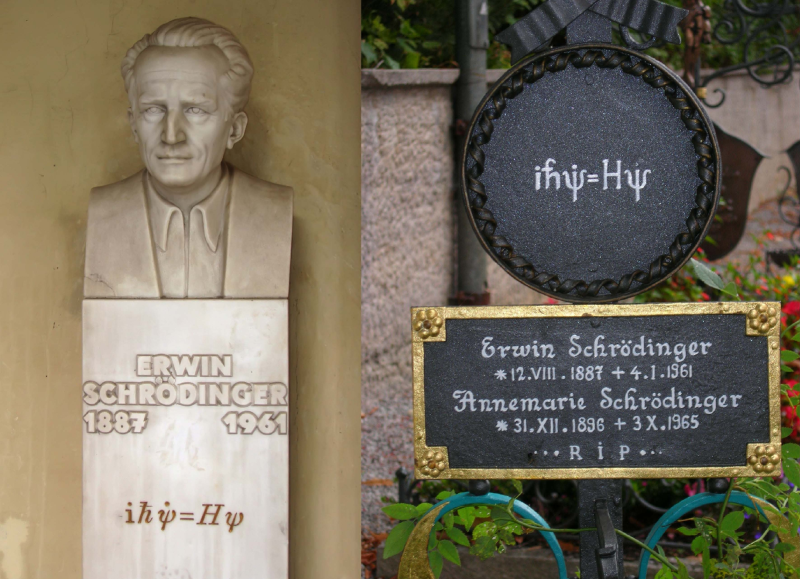
Figure 4. The Schrödinger equation — University of Vienna (left) and Alpbach (right), respectively.

Appendix A Summary of the Nikiforov–Uvarov method

Generalized equation of the hypergeometric type

$$u^{\prime\prime}+\frac{\widetilde{\tau}(x)}{\sigma(x)}u^{\prime}+\frac{\widetilde{\sigma}(x)}{\sigma^{2}(x)}u=0$$ (A.1)

($\sigma,$ $\widetilde{\sigma}$ are polynomials of degrees at most $2,\widetilde{\tau}$ is a polynomial at most first degree) by the substitution

$$u=\varphi(x)y(x)$$ (A.2)

can be reduced to the form

$$\sigma(x)y^{\prime\prime}+\tau(x)y^{\prime}+\lambda y=0$$ (A.3)

if:

$$\frac{\varphi^{\prime}}{\varphi}=\frac{\pi(x)}{\sigma(x)},\qquad\pi(x)=\frac{1}{2}\left(\tau(x)-\widetilde{\tau}(x)\right)$$ (A.4)

(or, $\tau(x)=\widetilde{\tau}+2\pi,$ for later),

$$k=\lambda-\pi^{\prime}(x)\qquad(\text{or, }\lambda=k+\pi^{\prime}),$$ (A.5)

and

$$\pi(x)=\frac{\sigma^{\prime}-\widetilde{\tau}}{2}\pm\sqrt{\left(\frac{\sigma^{\prime}-\widetilde{\tau}}{2}\right)^{2}-\widetilde{\sigma}+k\sigma}$$ (A.6)

is a linear function. (Use the choice of constant $k$ to complete the square under the radical sign; see [44] and our note below for more details.)

In Nikiforov–Uvarov’s method, the energy levels can be obtained from the quantization rule:

$$\lambda+n\tau^{\prime}+\frac{1}{2}n\left(n-1\right)\sigma^{\prime\prime}=0\qquad(n=0,1,2,\ ...)$$ (A.7)

and the corresponding square-integrable solutions are classical orthogonal polynomials, up to a factor. They can be found by the Rodrigues-type formula [44]:

$$y_{n}(x)=\dfrac{B_{n}}{\rho(x)}\left(\sigma^{n}(x)\rho(x)\right)^{(n)},\qquad(\sigma\rho)^{\prime}=\tau\rho,$$ (A.8)

where $B_{n}$ is a constant (see also [58]).

The corresponding data for the nonrelativistic and relativistic hydrogenlike problems are presented in Tables 1 and 2, respectively.

$\sigma(x)$	$x$
$\widetilde{\sigma}(x)$	$2\varepsilon_{0}\;x^{2}+2Z\;x-l\left(l+1\right)\/,\quad{\varepsilon_{0}=E/E_{0}}$
$\widetilde{\tau}(x)$	$0$
$k$	$2Z-\left(2l+1\right)\sqrt{-2\varepsilon_{0}\/}$
$\pi\left(x\right)$	$l+1-\sqrt{-2\varepsilon_{0}}\;x$
$\tau\left(x\right)=\widetilde{\tau}+2\pi\qquad$	$2\left(l+1-\sqrt{-2\varepsilon_{0}}\;x\right)$
$\lambda=k+\pi^{\prime}$	$2\left(Z-(l+1)\sqrt{-2\varepsilon_{0}}\right)$
$\varphi\left(x\right)$	$x^{l+1}e^{-x\sqrt{-2\varepsilon_{0}}}$
$\rho(x)$	$x^{2l+1}e^{-(2Z\ x)/n},\quad x=r/a_{0}$
$y_{n_{r}}(x)$	$C_{n_{r}}L_{n_{r}}^{2l+1}\left(\eta\right),\quad\eta=\dfrac{2Z}{n}x=\dfrac{2Z}{n}\left(\dfrac{r}{a_{0}}\right)$
$C_{n_{r}}^{2}$	$\dfrac{Z}{a_{0}n^{2}}\dfrac{\left(n-l-1\right)!}{\left(n+l\right)!},\quad n_{r}=n-l-1$

Table 1. Schrödinger equation for the Coulomb potential $V(r)=-\dfrac{Ze^{2}}{r}.$
Dimensionless quantities:
$$r=a_{0}x,\quad a_{0}=\frac{\hbar^{2}}{m_{e}e^{2}}\simeq 0.5\cdot 10^{-8}\;\text{cm},\quad E_{0}=\frac{e^{2}}{a_{0}};\quad R\left(r\right)=F\left(x\right)=\frac{u\left(x\right)}{x}.$$

$\sigma(x)$	$x$
$\widetilde{\sigma}(x)$	$\left(\varepsilon^{2}-1\right)\;x^{2}+2\mu\varepsilon\;x+\mu^{2}-l\left(l+1\right)$
$\widetilde{\tau}(x)$	$0$
$k$	$2\mu\varepsilon-\left(2\nu+1\right)\sqrt{1-\varepsilon^{2}},\quad\nu=-\dfrac{1}{2}+\sqrt{\left(l+\dfrac{1}{2}\right)^{2}-\mu^{2}}$
$\pi\left(x\right)$	$\nu+1-a\;x,\qquad a=\sqrt{1-\varepsilon^{2}}$
$\tau\left(x\right)=\widetilde{\tau}+2\pi$	$2\left(\nu+1-a\;x\right)$
$\lambda=k+\pi^{\prime}$	$2\left(\mu\varepsilon-(\nu+1)a\right)$
$\varphi\left(x\right)$	$x^{\nu+1}e^{-a\ x}$
$\rho(x)$	$x^{2\nu+1}e^{-2a\ x}$
$y_{n_{r}}(x)$	$C_{n_{r}}L_{n_{r}}^{2\nu+1}\left(\xi\right),\quad\xi=2ax=2a\beta r=2\sqrt{1-\varepsilon^{2}}\dfrac{mc}{\hbar}r$
$C_{n_{r}}$	$2\left(a\beta\right)^{3/2}\left(2a\right)^{\nu}\sqrt{\dfrac{n_{r}!}{(\nu+n_{r}+1)\Gamma\left(2\nu+n_{r}+2\right)}}$

Table 2. Relativistic Schrödinger equation for the Coulomb potential $V(r)=-\dfrac{Ze^{2}}{r}.$
Dimensionless quantities:
$$\varepsilon=\frac{E}{mc^{2}},\quad x=\beta r=\frac{mc}{\hbar}r,\quad\mu=\frac{Ze^{2}}{\hbar c};\qquad R\left(r\right)=F\left(x\right)=\frac{u\left(x\right)}{x}.$$

Note. A closed form for the constant $k$ can be obtained as follows. Let

$$p(x)={\left(\frac{\sigma^{\prime}-\widetilde{\tau}}{2}\right)^{2}-\widetilde{\sigma}+k\sigma}=q(x)+k\sigma(x)\/,$$ (A.9)

where

$$q(x)=\left(\frac{\sigma^{\prime}-\widetilde{\tau}}{2}\right)^{2}-\widetilde{\sigma}\/.$$ (A.10)

Completing the square, one gets

$$p(x)=\dfrac{p^{\prime\prime}}{2}\left(x+\frac{p^{\prime}(0)}{p^{\prime\prime}}\right)^{2}-\dfrac{\left(p^{\prime}(0)\right)^{2}-2p^{\prime\prime}p(0)}{2p^{\prime\prime}}\/,$$ (A.11)

where the last term must be eliminated:

$${\left(p^{\prime}(0)\right)^{2}-2p^{\prime\prime}p(0)}=0\/.$$ (A.12)

Therefore,

$$\left(q^{\prime}(0)+k\sigma^{\prime}(0)\right)^{2}-2\left(q^{\prime\prime}+k\sigma^{\prime\prime}\right)\left(q(0)+k\sigma(0)\right)=0\/,$$ (A.13)

which results in the following quadratic equation:

$$ak^{2}+2bk+c=0.$$ (A.14)

Here,

$$a=\left(\sigma^{\prime}(0)\right)^{2}-2\sigma^{\prime\prime}\sigma(0)\/,$$ (A.15)

$$b=q^{\prime}(0)\sigma^{\prime}(0)-\sigma^{\prime\prime}q(0)-\sigma(0)q^{\prime\prime}\/,$$ (A.16)

$$c=\left(q^{\prime}(0)\right)^{2}-2q^{\prime\prime}q(0)\/.$$ (A.17)

Solutions are

$$k_{0}=-\dfrac{c}{2b},\qquad\text{if}\quad a=0$$ (A.18)

and

$$k_{1,2}=\dfrac{-b\pm\sqrt{d}}{a},\qquad\text{if}\quad a\neq 0\/.$$ (A.19)

Here,

$$d=b^{2}-ac=\left(\sigma(0)q^{\prime\prime}+\sigma^{\prime\prime}q(0)\right)^{2}-2\left(\sigma^{\prime}(0)q^{\prime\prime}-\sigma^{\prime\prime}q^{\prime}(0)\right)\left(\sigma(0)q^{\prime}(0)-\sigma^{\prime}(0)q(0)\right)\/.$$ (A.20)

As a result,

$$p(x)=\left(\dfrac{p^{\prime\prime}}{2}\left(x+\frac{p^{\prime}(0)}{p^{\prime\prime}}\right)^{2}\right)_{k=k_{0,1,2}}\/,$$ (A.21)

which allows evaluating linear function $\pi(x)\/$ in the Nikiforov–Uvarov technique. (Examples are presented in Tables 1 and 2.)

Appendix B Evaluation of the integral

Integrating by parts on the right-hand side of (5.8), one gets

$${\left.\int_{r_{1}}^{r_{2}}p(r)\,dr=rp(r)\right|}_{r_{1}}^{r_{2}}-\int_{r_{1}}^{r_{2}}\dfrac{r\left[-(B/r^{2})+2(C/r^{3})\right]}{2p(r)}\,dr$$ (B.1)

$$\quad=\dfrac{B}{2}\int_{r_{1}}^{r_{2}}\dfrac{dr}{\sqrt{-Ar^{2}+Br-C}}-\int_{r_{1}}^{r_{2}}\dfrac{(C/r^{2})\,dr}{\sqrt{-A+(B/r)-(C/r^{2})}}\/.$$

For the last but one integral, we can write

$$\int_{r_{1}}^{r_{2}}\dfrac{dr}{\sqrt{\left(\frac{B^{2}}{4{A}}-C\right)-\left(r\sqrt{A}-\frac{B}{2\sqrt{A}}\right)^{2}}}\/={\left.\dfrac{1}{\sqrt{A}}\arcsin\dfrac{r\sqrt{A}-\frac{B}{2\sqrt{A}}}{{\sqrt{\frac{B^{2}}{4A}-C}}}\right|}_{r_{1}}^{r_{2}}=\dfrac{\pi}{\sqrt{A}}\ .$$ (B.2)

The following substitution $r=1/x\/,$ in the last integral of (B.1), results in

$$-\int_{x_{1}=1/{r_{1}}}^{x_{2}=1/{r_{2}}}\dfrac{C\,dx}{\sqrt{-A+Bx-Cx^{2}}}=-\sqrt{C}\int_{x_{1}}^{x_{2}}\dfrac{\sqrt{C}\,dx}{\sqrt{\left(\frac{B^{2}}{4C}-A\right)-\left(x\sqrt{C}-\frac{B}{2\sqrt{C}}\right)^{2}}}=\pi\,\sqrt{C}\/,$$ (B.3)

where we have completed the square and performed a familiar integral evaluation. (One may also interchange $A$ and $C$ in the previous integral evaluation.) Combining the last two integrals, one can complete the proof.

Appendix C The Laplace method

The second order ordinary differential equation with linear coefficients,

$$L[u]:=x\dfrac{d^{2}u}{dx^{2}}+\left(\delta_{0}x+\delta_{1}\right)\dfrac{du}{dx}+\left(\varepsilon_{0}x+\varepsilon_{1}\right)u=0\/,$$ (C.1)

the so-called Laplace equation, is easy to handle for the following reason: the Laplace transform gives an equation of the first order [48], [49]. Letting

$$u(x)=\int_{C}e^{xz}v(z)\,dz$$ (C.2)

one gets

$$xu^{\prime\prime}+\delta_{0}xu^{\prime}+\varepsilon_{0}xu=x\int_{C}e^{xz}\left[\left(z^{2}+\delta_{0}z+\varepsilon_{0}\right)v(z)\right]\,dz$$

$$\quad=\int_{C}\dfrac{d}{dz}\left(e^{xz}\right)\left[\left(z^{2}+\delta_{0}z+\varepsilon_{0}\right)v(z)\right]\,dz$$

$$\quad=\int_{C}\dfrac{d}{dz}\left[e^{xz}\left(z^{2}+\delta_{0}z+\varepsilon_{0}\right)v(z)\right]\,dz$$

$$\qquad-\int_{C}e^{xz}\dfrac{d}{dz}\left[\left(z^{2}+\delta_{0}z+\varepsilon_{0}\right)v(z)\right]\,dz$$ (C.3)

and

$$\delta_{1}u^{\prime}+\varepsilon_{1}u=\int_{C}e^{xz}\left[\left(\delta_{1}z+\varepsilon_{1}\right)v(z)\right]\,dz\/.$$ (C.4)

Thus

$$L[u](x)=\int_{C}\dfrac{d}{dz}\left[e^{xz}\left(z^{2}+\delta_{0}z+\varepsilon_{0}\right)v(z)\right]\,dz$$

$$\qquad\quad-\int_{C}e^{xz}\dfrac{d}{dz}\left[\left(z^{2}+\delta_{0}z+\varepsilon_{0}\right)v(z)\right]\,dz$$

$$\qquad\qquad+\int_{C}e^{xz}\left[\left(\delta_{1}z+\varepsilon_{1}\right)v(z)\right]\,dz\equiv 0\/$$ (C.5)

provided

$$\dfrac{d}{dz}\left[\left(z^{2}+\delta_{0}z+\varepsilon_{0}\right)v(z)\right]=\left(\delta_{1}z+\varepsilon_{1}\right)v(z)$$ (C.6)

and the corresponding boundary condition holds.

Let $c_{1}$ and $c_{2}$ be roots of the following quadratic equation:

$$z^{2}+\delta_{0}z+\varepsilon_{0}=(z-c_{1})(z-c_{2})=0\/.$$ (C.7)

Denoting $v_{1}(z)=(z-c_{1})(z-c_{2})v(z)\/,$ we obtain

$$\dfrac{v_{1}^{{}^{\prime}}(z)}{v_{1}(z)}=\dfrac{\delta_{1}z+\varepsilon_{1}}{(z-c_{1})(z-c_{2})}=\dfrac{\alpha_{1}}{z-c_{1}}+\dfrac{\alpha_{2}}{z-c_{2}}\/,$$ (C.8)

where

$$\alpha_{1}=\dfrac{c_{1}\delta_{1}+\varepsilon_{1}}{c_{1}-c_{2}}\/,\qquad\alpha_{2}=\dfrac{c_{2}\delta_{1}+\varepsilon_{1}}{c_{2}-c_{1}}\/.$$ (C.9)

As a result, one gets

$$v(z)=(z-c_{1})^{\alpha_{1}-1}(z-c_{2})^{\alpha_{2}-1}\/$$ (C.10)

and our solution take the form

$$u(x)=\int_{C}e^{xz}(z-c_{1})^{\alpha_{1}-1}(z-c_{2})^{\alpha_{2}-1}\,dz$$ (C.11)

provided that the following holds for the contour $C$:

$$\int_{C}\dfrac{d}{dz}\left[e^{xz}(z-c_{1})^{\alpha_{1}}(z-c_{2})^{\alpha_{2}}\right]\,dz=0\/.$$ (C.12)

For original applications of this method to the Coulomb problems see [49] and [20]; more historical details are available in [39], pp. 426–434.

According to the original Schrödinger rudimentary quantization rule, the exponents ${\alpha_{1}}$ or ${\alpha_{2}}$ in the above complex integral solution were required to be negative integers. In his letter to Sommerfeld, Schrödinger wrote with excitement that “Finally I wish to add that the discovery of the whole connection [between the wave equation and the quantization of hydrogen atom], goes back to your beautiful quantization method for evaluating the radial quantum integral. … which suddenly shone out from the exponents ${\alpha_{1}}$ and ${\alpha_{2}}$ like a Holy Grail.” (see [39], p. 462 or [40], p. 172).

Appendix D A Letter from Schrödinger to Weyl

Berlin-Grunewald, 1. April 1931
[Typescript]

Dear Mr. Weyl,

Once again, I have let pass a long period of time, in a completely unproportional way, before hereby saying thanks for your prestigious, beautiful present – the second edition of your book. I have found most interesting the new presentation of Dirac’s theory since I am dealing with it currently. As far as I can see, you have decided to use a new terminology since you consider the following as important: to express that one can arrange that the Dirac matrices – with the unique exception of the mass term – transform in such a way the first couple and the second couple of the components of $\psi$ among themselves, and moreover, that this property also holds with respect to an arbitrary Lorenz transform. One can perceive (and you mention this somewhere in the text) that your hope focusses on the fact that all the four components and equations correspond to the electron and proton. I wish that this hope might become fulfilled very soon. [The “right” antiparticle – positron will be discovered only next year!]

May I tell you about some vague thoughts which confirm my impressions about this? If you consider the components of the “current” as “a probability for the electron propagation process through the area element” then one can explicitly say that this is – similar to the gas kinetic diffusion theory – a difference of the probability for passing in one way or the other. Something similar then must hold for the density. Certain points which can classically be considered as the trace of a world line, perforating the volume element, must be considered as positive, others as negative. This means the density must be in connection with the algebraic sum of charges. This fact must be applicable to electrons as well as protons – we should point out however that the current density then has four perforation points – what at first sight is somehow perturbing – or alternatively, one has to assume something like the theory of holes, like it is done by Dirac. Within such a theory, the world lines of protons are really in a certain sense world lines which pass from the future back towards the past. Namely if such a hole spatially propagates from $A$ to $B,$ then you will find the following situation: before the process, there is nothing in $A$ but something in $B.$ Afterwards, there is something in $A$ but nothing in $B.$ (Is one allowed to call this inverted time direction, or is it simply inverted spatial direction?)

I have to say that I am quite astonished about the following: I have more difficulties to read your written words than to follow your speech. I believe it is related to the fact that mathematical objects and conclusions are much more apparent to you than to many other people. Hence you eliminate steps in a chain of thoughts which would be necessary for others to be included. Like in the prominent example: “A man thinks that men are dangerous.” It would be disgusting to add here the following conclusion: “Consequently, this man is dangerous”. I think that your aesthetical perception – which would avoid and not allow such a conclusion – is an obstacle for you, to summarize with primitive words at the end again what has been derived and what has been proven.

I am most thankful for the register of operations symbols and symbols with a fixed meaning. This constitutes an enormous relaxation in contrast to the first edition.

Moreover I see that many, many things are new, being an enormous extension of the first edition which remains in some aspects just not accessible to me, taking into regards my abilities to understand it. In my brain, understanding quantum mechanics takes place at such a slow speed – and slower than in the case of any other man. Ehrenfest’s picture of a small asthmatic dachshund – breathless following Electra – can be applied to full extent to myself. Perhaps I will understand all the quantum facts precisely at the moment when they will no more be valid.

One smaller aspect: on page 119, one finds the expression of intersection of two subgroups. However this expression is not available in the index of the book. It is, as far as I can see, for the first time present on page 105, but also there, it is not explained explicitly.

A slight deviation, not following the main stream of the approach, I can moreover find in comparing page 99, line 4 from above (“From now on … only the one-to-one maps.”) and page 120, line 7 from above, where as far as I can see, a definition of mapping is needed which is non unique.

I still have another point, and I hope you will not mind. As for the headline of paragraphs 2 and 3 in chapter 2, you chose the names de Broglie and Schrödinger. It looks as if the first one knew about the assignment of operators and the wave equation in a space without fields, but not about the curvature of rays in a potential field. And moreover it looks as if it was the second one who has respected the influence of the field by having introduced the potentials into the wave equation. I do not think that this is a consequent way of argumentation. If you hold the view that the approach by de Broglie with respect to ray propagation and wavelength constitute already a description of the wave equation (even given the fact that he does not write it down with algebraic symbols), then you will have to assign the wave equation, including potentials, under the name “de Broglie”. The reason for this is the following: the behavior of the objects in the field was known to him as well as the behavior of the objects in a field-free space – without a single jota difference in his perception. On the other hand, it is indeed somewhat disturbing to find the operator assignment $(p_{1}\to\partial/\partial q_{1})$ – which to my knowledge has really been communicated for the first time in my manuscript from 18th March 1926 – being assigned to his name. The same perception applies to the scalar relativistic equation which I have described on the first page of my first treatment (although having used just written words). About its solution, I have made some remarks in paragraph 3, and 2 of the same publication. I have never expressed any protest against the fact that this equation now is correlated with the name Gordon, since this helps determining the different scenarios. But I do not like to see them being assigned to the name de Broglie – for obvious reasons (compare for instance also with page 188 of your book).

Please do not mind my objections, I hate deliberations of this type like the death, I am not angry, nor offended or insulted. I know that something like this may happen if one tries to order the thoughts behind given facts to one concluding, consequent, compact stream of perception. While doing so, one has often to separate what is united from the viewpoint of its historical origin. And on the other hand, hand one has to unify what is historically separated. One should avoid telling: this one has made this and that one has made that. In principle, all that is equivalent. I have no doubt that you will understand my impression to a certain extent and you will not decline its meaning to a certain extent.

And please, it would be horrible if you believe you would have to submit now declarations and justifications. This is not my intention. I just wanted to talk about it. It is not that important – so let me end my deliberations there.

You are just returning from the USA, and hopefully you have had two pleasant and not too stormy crossings overseas. I am little bit jealous about your travels overseas (even in case they were stormy). But I am not too jealous about your stay in the US. But just for 14 days, I would like to travel there if there is an opportunity, i. e. if someone else is going to pay for it. 14 days on a ship is the most beautiful and most recovering Easter holiday – well, it costs something.

With the most cordial greetings and hand kisses from house to house
Yours sincerely     Schrödinger

Acknowledgments. We are grateful to Prof. Dr. Ruben Abagyan, Dr.  Mark Faifman, Prof. Dr.  Yakov I. Granovskiĭ, Prof. Dr. Georgy T. Guria, Prof. Dr. Christian Krattenthaler, Dr. Sergey I. Kryuchkov, Prof. Dr. Peter Paule, Dr. Naya Smorodinskaya, Dr. Eugene Stepanov, and Prof. Dr. Alexei Zedanov for support, help, and valuable comments. We are indebted to the referees, their comments helped us to improve the manuscript.

References

- [1] H. A. Bethe and E. E. Salpeter, Quantum Mechanics of One- and Two- Electron Atoms, Berlin, Heidelberg: Springer, 1957. DOI: 10.1007/978-3-662-12869-5; reprinted by Dover, 2008.
- [2] F. Bloch, Heisenberg and the early days of quantum mechanics, Physics Today 29 no. 12 (1976), 23–27. DOI: 10.1063/1.3024633.
- [3] D. I. Blokhintsev, Quantum Mechanics, Dordrecht: Springer Netherlands, 1964. DOI: 10.1007/978-94-010-9711-6.
- [4] D. I. Blokhintsev, Classical statistical physics and quantum mechanics, Soviet Physics Uspekhi 20 no. 8 (1977), 683–690. DOI: 10.1070/pu1977v020n08abeh005457.
- [5] L. de Broglie, Sur la fréquence propre de l’électron, Comptes Rendus 180 (1925), 498–500.
- [6] D. C. Cassidy, Uncertainty: The Life and Science of Werner Heisenberg, New York, N. Y.: W. H. Freeman and Company, 1991.
- [7] D. C. Cassidy, Beyond Uncertainty : Heisenberg, Quantum Physics, and the Bomb, New York, N. Y. : Bellevue Literary Press, 2009.
- [8] R. Courant and D. Hilbert, Methoden der mathematischen Physik, Berlin: Springer, 1924. (First German edition.) Methods of Mathematical Physics, 1, Hoboken, Jew Jersey: John Wiley & Sons, Inc., 1989. (Fifth English edition.) DOI: 10.1002/9783527617210
- [9] O. Darrigol, A few reasons why Louis de Broglie discovered matter waves and yet did not discover Schrödinger’s equation, in Erwin Schrödinger — 50 Years After (W. L. Reiter and J. Yngvason, eds.), EMS ESI Lectures in Mathematics and Physics vol 9, Zürich: European Mathematical Society Publishing House, Switzerland, 2013, pp. 165–174. DOI: 10.4171/121.
- [10] C. G. Darwin, The wave equations of the electron, Proceedings of the Royal Society of London. Series A, Containing Papers of a Mathematical and Physical Character 118 no. 780 (1928), 654–680. DOI: 10.1098/rspa.1928.0076.
- [11] A. S. Davydov, Quantum Mechanics, International series of monographs in natural philosophy 1, Oxford : Pergamon Press, 1965.
- [12] P. A. M. Dirac, The quantum theory of the electron, Proceedings of the Royal Society of London. Series A, Containing Papers of a Mathematical and Physical Character 117 no. 778 (1928), 610–624. DOI: 10.1098/rspa.1928.0023.
- [13] P. A. M. Dirac, The evolution of the physicist’s picture of nature, Scientific American 208 no. 5 (1963), 45–53. http://www.jstor.org/stable/24936146 . See also, My life as a physicist, in Unity of the Fundamental Interactions (A. Zichichi, ed.), New York and London: Plenum Press, 1983, pp. 740–741. https://www.springer.com/gp/book/9780306412424.
- [14] P. A. M. Dirac, The relativistic electron wave equation, Sov. Physics Uspekhi 22 no. 8 (1979), 648–653. DOI: https://doi.org/10.1070/PU1979v022n08ABEH005593
- [15] P. A. M. Dirac, The Principles of Quantum Mechanics, 4 ed., Oxford, UK: Clarendon Press, (1958)1967.
- [16] F. Dyson, Birds and Frogs, Notices of the AMS 56 no. 2 (2009), 212–223; Birds and Frogs in Mathematics and Physics, revised for Physics Uspekhi 180 no. 8 (2009), 859–870 [in Russian]. DOI: 10.3367/UFNe.0180.201008f.0859
- [17] A. Einstein, Letters on Wave Mechanics: Correspondence with H. A. Lorentz, Max Planck, and Erwin Schrödinger, (K. Przibram, ed.), New York: Open Road Integrated Media, (1967)2011.
- [18] M. A. El’yashevich, From the origin of quantum concepts to the establishment of quantum mechanics, Soviet Physics Uspekhi 20 no. 8 (1977), 656–682. DOI: 10.1070/pu1977v020n08abeh005456.
- [19] G. Farmelo, The Strangest Man: The Hidden Life of Paul Dirac, Mystic of the Atom, New York: Basic Books, 2009.
- [20] V. Fock, Zur Schrödingerschen Wellenmechanik, Zeitschrift für Physik 38 no. 3 (1926), 242–250, [in German] (received June 11, published July 28); reprinted in V. A. Fock, Selected Works: Quantum Mechanics and Quantum Field Theory. (L. D. Faddeev, L. A. Khalfin, and I. V. Komarov, eds.), Boca Raton, London, New York, Washington, D. C. : Chapman & Hill /CRC, 2004, pp. 11–20. DOI: 10.1007/BF01399113.
- [21] V. Fock, Über die invariante Form der Wellen- und der Bewegungsgleichungen für einen geladenen Massenpunkt, Zeitschrift für Physik 39 no. 2/3 (1926), 226–232, [in German] (received July 30, published October 2); reprinted in V. A. Fock, Selected Works: Quantum Mechanics and Quantum Field Theory. (L. D. Faddeev, L. A. Khalfin, and I. V. Komarov, eds.), Boca Raton, London, New York, Washington, D. C. : Chapman & Hill /CRC, 2004, pp. 21–28. DOI: https://doi.org/10.3367/UFNe.0180.201008h.0874. See also, L. B. Okun, V. A. Fock and gauge invariance, Soviet Physics Uspekhi 53 no. 8 (2010), 835–838. DOI: https://doi.org/10.3367/UFNe.0180.201008g.0871.
- [22] V. A. Fock, Fundamentals of Quantum Mechanics, Moscow: Mir Publishers, 1978. https://mirtitles.org/2013/01/01/fock-fundamentals-of-quantum-mechanics/
- [23] W. Gordon, Die Energieniveaus des Wasserstoffatoms nach der Diracschen Quantentheorie des Elektrons, Zeitschrift für Physik 48 no. 1 (1928), 11–14, [in German]. DOI: 10.1007/BF01351570.
- [24] Y. I. Granovskiĭ, Sommerfeld formula and Dirac’s theory, Physics-Uspekhi 47 no. 5 (2004), 523–524. DOI: 10.1070/pu2004v047n05abeh001885.
- [25] J. Gribbin, Erwin Schrödinger and the Quantum Revolution, 1 ed., Hoboken, Jew Jersey: John Wiley & Sons, Inc., 2012.
- [26] C. Joas and C. Lehrer, The classical roots of wave mechanics: Schrödinger’s transformations of the optical-mechanical analogy, Studies in History and Philosophy of Science Part B: Studies in History and Philosophy of Modern Physics 40 no. 4 (2009), 338–351. https://doi.org/10.1016/j.shpsb.2009.06.007.
- [27] W. Hesenberg, The Physical Principals of the Quantum Theory, New York: Dover Publications, 1949.
- [28] P. L. Kapitza, Experiment, Theory, Practice: Articles and Addresses, Dordrecht, Boston, London: Reidel, 1980, pp. 318–319.
- [29] A. J. Kox, The debate between Hendrik A. Lorentz and Schrödinger on wave mechanics, in Erwin Schrödinger — 50 Years After (W. L. Reiter and J. Yngvason, eds.), EMS ESI Lectures in Mathematics and Physics vol 9, Zürich: European Mathematical Society Publishing House, Switzerland, 2013, pp. 153–162. DOI: 10.4171/121.
- [30] H. Kragh, Erwin Schrödinger and the wave equation: the crucial phase, Centaurus 26 no. 2 (1982), 154–197. DOI: 10.1111/j.1600-0498.1982.tb00659.x.
- [31] S. I. Kryuchkov, N. A. Lanfear, and S. K. Suslov, The role of the Pauli–Lubański vector for the Dirac, Weyl, Proca, Maxwell and Fierz–Pauli equations, Physica Scripta 91 no. 3 (2016), 035301. DOI: 10.1088/0031-8949/91/3/035301.
- [32] S. I. Kryuchkov, S. K. Suslov, and J. M. Vega-Guzmán , The minimum-uncertainty squeezed states for atoms and photons in a cavity, Journal of Physics B: Atomic, Molecular and Optical Physics 46 no. 10 (2013), 104007 (15pp). (IOP Highlights of 2013.) DOI: https://doi.org/10.1088/0953-4075/46/10/104007.
- [33] L. D. Landau and E. M. Lifshitz, Quantum Mechanics: Non-Relativistic Theory, 3 ed., Oxford, UK: Butterworth-Heinemann, (1977)1998, Revised and Enlarged. DOI: 10.1016/C2013-0-02793-4.
- [34] R. E. Langer, On the connection formulas and the solutions of the wave equation, Physical Review 51 no. 8 (1937), 669–676. DOI: 10.1103/PhysRev.51.669.
- [35] J. Mehra, The discovery of electron spin, in [38], 1, pp. 585–611. DOI: 10.1142/9789812810588_0017.
- [36] J. Mehra, Birth of quantum mechanics, in Werner Heisenberg Memorial Lecture Delivered at the CERN Colloquium on March 30, 1976, CERN, Geneva, 1976, reprinted in [38], 2, pp. 639–667. DOI: 10.1142/9789812810588_0019.
- [37] J. Mehra, Schrödinger and the rise of wave mechanics. II. The creation of wave mechanics, in [38], 2, pp. 761–802. DOI: 10.1142/9789812810588_0022.
- [38] J. Mehra, The Golden Age of Theoretical Physics, (Boxed Set of 2 Volumes), Singapore, New Jersey, London, Hong Kong: World Scientific, February 2001. DOI: 10.1142/4454.
- [39] J. Mehra and H. Rechenberg, The Historical Development of Quantum Theory, in Part 2 The Creation of Wave Mechanics; Early Response and Applications 1925–1926, Erwin Schrödinger and the Rise of Wave Mechanics 5, New York, N. Y.: Springer, 1 ed., 1987.
- [40] K. von Meyenne, Eine Entdeckung vonanz auerordentlecher Tragweite: Schrödingers Briefwechsel zur Wellenmechanik und zum Katzenparadoxon, Berlin, Heidelberg : Springer, 2011. DOI: 10.1007/978-3-642-04335-2
- [41] V. P. Milant’ev, Creation and development of Bohr’s theory (on the 90th anniversary of the Bohr theory of the atom), Physics Uspekhi 47 no. 2 (2004), 197–203. DOI: 10.1070/PU2004v047n02ABEH001682.
- [42] A. I. Miller, Erotica, aesthetics and Schrödinger’s wave equation, in It Must Be Beautiful: Great Equations of Modern Science, (G. Farmelo, ed.), London: Granta Publications, 2002, pp. 110–131.
- [43] W. J. Moore, Schrödinger: Life and Thought, Cambridge: Cambridge University Press, 1989.
- [44] A. F. Nikiforov and V. B. Uvarov, Special Functions of Mathematical Physics: A Unified Introduction with Applications, Boston, MA: Birkhäuser, 1988. DOI: 10.1007/978-1-4757-1595-8.
- [45] S. V. Petrov, Was Sommerfeld wrong?, Physics Uspekhi 63 no. 7 (2020), 721–724. DOI: https://doi.org/10.3367/UFNe.2019.11.038695
- [46] J. Renn, Schrödinger and the genesis of wave mechanics, in Erwin Schrödinger — 50 Years After (W. L. Reiter and J. Yngvason, eds.), EMS ESI Lectures in Mathematics and Physics vol 9, Zürich: European Mathematical Society Publishing House, Switzerland, 2013, pp. 9–36. DOI: 10.4171/121.
- [47] L. I. Schiff, Quantum Mechanics, 3 ed., New York: McGraw-Hill, 1968.
- [48] L. Schlesinger, Einführung in die Theorie der Differentialgleichungen mit einer unabhängigen Variabeln, Summlung Schubert, No. XIII, Leipzig : G. J. Göschenshe Verlagshandlung, 1900.
- [49] E. Schrödinger, Quantisation as a problem of proper values (Part I), in Collected Papers on Wave Mechanics, New York, Providence, Rhode Island: AMS Chelsea Publishing, 2010, (Original: Annalen der Physik (4), vol. 79(6), pp. 489–527, 1926 [in German]), pp. 1–12.
- [50] E. Schrödinger, Quantisation as a problem of proper values (Part II), in Collected Papers on Wave Mechanics, New York, Providence, Rhode Island: AMS Chelsea Publishing, 2010, (Original: Annalen der Physik (4), vol. 79(6), pp. 489–527, 1926 [in German]), pp. 13–40.
- [51] E. Schrödinger, The continuous transition from micro-to macro-mechanics, in Collected Papers on Wave Mechanics, 28, New York, Providence, Rhode Island: AMS Chelsea Publishing, 2010, (Original: Die Naturwis-senschaften, vol. 28, pp. 664–666, 1926 [in German]), pp. 41–44.
- [52] E. Schrödinger, On the relation between the quantum mechanics of Heisenberg, Born, and Jordan, and that of Schrödinger, in Collected Papers on Wave Mechanics, New York, Providence, Rhode Island: AMS Chelsea Publishing, 2010, (Original: Annalen der Physik (4), vol. 79(8), pp. 734–756, 1926 [in German]), pp. 45–61.
- [53] E. Schrödinger, Quantisation as a problem of proper values (Part IV), in Collected Papers on Wave Mechanics, New York, Providence, Rhode Island: AMS Chelsea Publishing, 2010, (Original: Annalen der Physik (4), vol. 81, pp. 109–139, 1926 [in German]), pp. 102–123.
- [54] E. Schrödinger, An undulatory theory of the mechanics of atoms and molecules, The Physical Review Second Series 28 no. 6 (1926), 1049–1070. https://doi-org.ezproxy1.lib.asu.edu/10.1103/PhysRev.28.1049; Soviet Physics Uspekhi 7 no. 3 (1927), 176–201 [in Russian]. DOI: DOI: 10.3367/UFNr.0007.192703b.0176
- [55] E. Schrödinger, Collected Papers on Wave Mechanics, 28, New York, Providence, Rhode Island: AMS Chelsea Publishing, 2010.
- [56] Ya. A. Smorodinskiĭ and T. B. Romanovskaya, Louis de Broglie (1892–1987), Soviet Physics Uspekhi 31 no. 12 (1988), 1080–1084. DOI: https://doi.org/10.1070/PU1988v031n12ABEH005661.
- [57] A. Sommerfeld, Atombau und Spektrallinien, 2 ed., 1, Friedrich Vieweg & Sohn, Braunschweig, German, 1951. [in German]
- [58] S. K. Suslov, J. M. Vega-Guzmán, and K. Barley, An introduction to special functions with some applications to quantum mechanics, in Orthogonal Polynomials: 2nd AIMS-Volkswagen Stiftung Workshop, Douala, Cameroon, 5-12 October, 2018 (M. Foupouagnigni and W. Koepf, eds.), Tutorials, Schools, and Workshops in the Mathematical Sciences no. AIMSVSW 2018, Springer Nature Switzerland AG, March 2020, pp. 517–628. DOI: 10.1007/978-3-030-36744-2_21.
- [59] D. A. Varshalovich, A. N. Moskalev, and V. K. Khersonskii, Quantum Theory of Angular Momentum, Singapore, New Jersey, Hong Kong: World Scientific, 1988. DOI: 10.1142/0270.
- [60] B. L. van der Waerden, (ed.), Sources of Quantum Mechanics, Classics of Science, v 5, New York: Dover Publications, 1968.
- [61] L. Wessels, Schrödinger’s route to wave mechanics, Studies in History and Philosophy of Science Part A 10 no. 4 (1979), 311–340. DOI: 10.1016/0039-3681(79)90018-9.
- [62] H. Weyl, The Theory of Group and Quantum Mechanics, New York: Dover Publications, 1950.