Partial Identifiability in Discrete Data With Measurement Error

Abstract

When data contains measurement errors, it is necessary to make assumptions relating the observed, erroneous data to the unobserved true phenomena of interest. These assumptions should be justifiable on substantive grounds, but are often motivated by mathematical convenience, for the sake of exactly identifying the target of inference. We adopt the view that it is preferable to present bounds under justifiable assumptions than to pursue exact identification under dubious ones. To that end, we demonstrate how a broad class of modeling assumptions involving discrete variables, including common measurement error and conditional independence assumptions, can be expressed as linear constraints on the parameters of the model. We then use linear programming techniques to produce sharp bounds for factual and counterfactual distributions under measurement error in such models. We additionally propose a procedure for obtaining outer bounds on non-linear models. Our method yields sharp bounds in a number of important settings – such as the instrumental variable scenario with measurement error – for which no bounds were previously known.

1 Introduction

Measurement error is a ubiquitous problem in fields ranging from epidemiology and public health [21, 1] to economics [15, 16, 17] to ecology [23, 22]. If unaccounted for during analysis, measurement error can lead biased results. Accounting for measurement error bias requires making assumptions about how errors occur so as to link the available data to the underlying true values. As such, it is important to the validity of the analysis and the resulting conclusions that these assumptions be substantively justifiable.

In practice, however, analysts often make implausibly strong assumptions for the sake of exactly identifying their target of inference. In such cases, we advocate instead for the use of weaker, credible assumptions to identify bounds on the target of inference, referred to as partial identification. Previous work on partial identifiability under measurement error has largely focused on deriving analytic bounds for specific combinations of settings and assumptions. As a result, there remain many important and common settings for which no known bounds exist.

In this work, we adopt a latent variable formulation of the measurement error problem. That is, we are interested in estimating a target parameter that involves the distribution of a discrete unobserved variable $X$ using observations of a discrete observed proxy variable $Y$. We show how sharp partial identification bounds for the target parameter can be computed numerically and without extensive derivations for a class of models, including several models for which no analytical bounds are currently known. Our approach, which is similar in spirit to that of [3], is to encode the target parameter and constraints imposed by the model as a linear program which can be maximized and minimized to produce sharp bounds. We show that this approach can be used to compute bounds for factual and counterfactual parameters of a discrete mismeasured variable, including its marginal distribution and its moments, and the average treatment effect (ATE) of an intervention on the mismeasured variable.

The primary contribution of this paper is a collection of modeling assumptions that can be encoded as linear constraints on a target parameter and, thus, are amenable to the linear programming approach. These include several common measurement error constraints (Section 2), graphical constraints encoded by hidden variable Bayesian networks (Section 3), and causal constraints relating potential outcomes under different interventions (Section 4). Our main result, presented in Section 3, draws on results from [11] and [9] to show how an extended class of instrumental variable-type models produce linear constraints on a target parameter and present a simple procedure for obtaining outer bounds for graphs outside this class.

Our approach allows a practitioner to mix and match any combination of the modeling assumptions described in this paper with little effort. This flexibility means that it is trivial to compute bounds under new models and to test the sensitivity of the resulting bounds to different combinations of assumptions. Throughout, we demonstrate the utility of this approach on synthetic examples representing important use cases. Our goal in these examples is to demonstrate how to apply the approach to commonly occurring models so that practitioners may adapt them to their specific data scenario. These cases include:

1. Bounding the mean of a variable using a single noisy proxy

2. Bounding the mean of a variable using two noisy proxies with an exclusion restriction

3. Bounding the ATE in a randomized trial with measurement error on the outcome

4. Bounding the ATE in an instrumental variable model with measurement error on the outcome

These cases represent common scenarios occurring in economics, public health, political science, and other scientific settings. Among these, cases 2, 3, and 4 all represent settings for which no sharp symbolic bounds are currently known and previous work suggests that deriving such symbolic bounds automatically for these settings is infeasible [5]. We begin by introducing our approach in the context of the simplest possible measurement error model (Section 2). Next, we describe a class a class of graphical models that yield linear constraints

2 The basic measurement error problem and the LP formulation

Suppose that we are interested in the distribution of a discrete random variable $X\in\mathcal{X}$, but instead of observing $X$ directly, we can only observe a discrete noisy proxy, denoted $Y\in\mathcal{Y}$. Clearly, without any assumptions about the proxy distribution, $P(Y|X)$, we cannot say anything about the distribution of $X$. On the opposite extreme, if $P(Y|X)$ is known and invertible, then $P(X)$ is fully identifiable from observations of $Y$ [21].

Our interest is in between these two extremes, where we assume certain properties of $P(Y|X)$, but not the whole distribution. Our goal is to bound functions of $P$, referred to as parameters of interest, under these assumptions. Our approach is to translate the modeling assumptions into a set of constraints on $P(X,Y)$ and bound the parameter of interest by finding its maximum and minimum subject to these constraints. Formally, let $\Delta^{d}$ be the $d$-dimensional simplex, let $\eta:\Delta^{|\mathcal{X}|\times|\mathcal{Y}|}\to\mathbb{R}$ be the parameter of interest, and let $\mathcal{M}\subseteq\Delta^{|\mathcal{X}|\times|\mathcal{Y}|}$ be the set of distributions allowed under the modeling assumptions. Then, assuming that $\mathcal{M}$ contains the true distribution $P_{0}$, we can bound $\eta(P_{0})$ as

$$\min_{P\in\mathcal{M}}\eta(P)\leq\eta(P_{0})\leq\max_{P\in\mathcal{M}}\eta(P)$$ (1)

We will show how to construct $\mathcal{M}$ such that this optimization problem is tractable and the bounds produced are sharp.

For notational simplicity, let $\phi_{xy}:=P(X=x,Y=y)$ be the joint distribution of $X$ and $Y$. By construction, $\phi$ must satisfy the the probability constraints $\sum_{xy}\phi_{xy}=1$, and for all $x,y$, $\phi_{xy}\geq 0$. In addition, $\phi$ must match the marginal for the observed proxy $Y$, so that for all $y$, $\sum_{x}\phi_{xy}=P(Y=y)$. These are called the observed data constraints.

As mentioned above, we must make assumptions about the relationship of the unobserved variable $X$ and the observed proxy $Y$. We seek to avoid strong, parametric assumptions, in favor of weaker assumptions that may be justified by expert knowledge or domain research. Below, we provide examples of several such commonly made assumptions. We call constraints on $\phi$ relating the proxies to the unobserved variables the measurement error constraints .

1. Bounded error proportion: $\sum_{x\neq y}\phi_{xy}\leq\epsilon$

2. Unidirectional errors: $\sum_{y<x}\phi_{xy}=0$

3. Symmetric error probabilities:
   $~{}~{}~{}~{}~{}\phi_{xy}=\phi_{xy}\,\,\,\forall\,\,|x-y|=|x-y^{\prime}|$

4. Error probabilities decrease by distance:
   $~{}~{}~{}~{}~{}\phi_{xy}\geq\phi_{xy^{\prime}}\,\,\,\forall\,\,|x-y|>|x-y^{\prime}|$

Assumption (A0) may be reasonable when there is sufficient previous literature to specify a range of plausible error rates, but not the exact proxy distribution (e.g., see discussion of sensitivity analysis in [21]). Assumption (A1) may be used to represent positive label only data, which is common in areas such as ecology [23] and public health [1]. Assumption (A2) represents a generalization of the zero-mean measurement error assumption – commonly made in settings where the errors are due to imprecision of the instrument – to discrete variables. Finally, Assumption (A3) may be reasonable in settings where the values of $X$ have a natural ordering and small errors are more likely than large ones.

Note that the target distribution $P(X=x)=\sum_{y}\phi_{xy}$ and all constraints described thus far can be written as linear functions of $\phi$. If our parameter of interest is also a linear function of $\phi$, then the assumed constraints, in combination with the linear objective corresponding to our parameter of interest, form a linear program (LP) and bounds can be computed by both maximizing and minimizing the parameter of interest using one of a number of LP solvers. Parameters that are linear in $\phi$ include $P(X)$ and all of its moments. By the intermediate value theorem, the objective can take any value between its constrained maximum and minimum values. It follows that for sets of assumptions that can be linearly expressed, the bounds obtained through this linear program are sharp, i.e. they exhaust the information in the observed data under the stated assumptions.

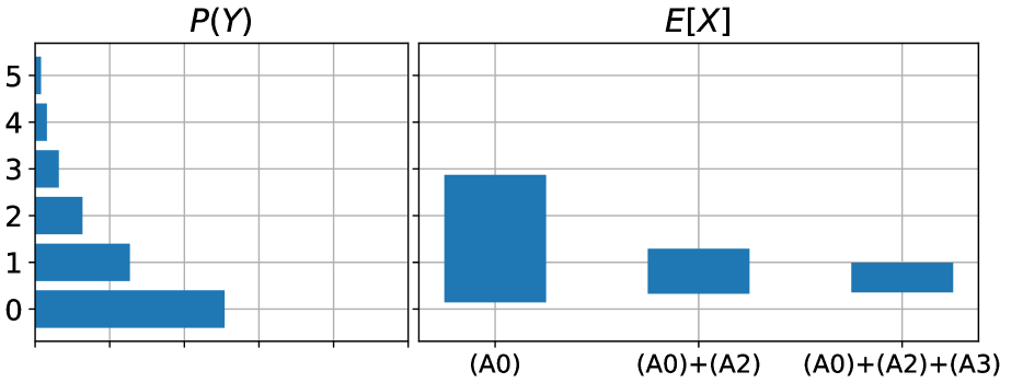
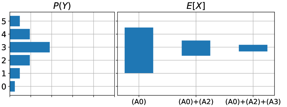
Figure 1: Bounds on $E[X]$ under different measurement error assumptions and observed proxy distributions, $P(Y)$.

Application: Bounding $E[X]$ using a single proxy

To demonstrate this approach, suppose we are interested in bounding the expected value of a variable $X\in\{0,..,5\}$ from observations of $Y\in\{0,...,5\}$. We will consider bounds under (A2), (A3), and a weaker version of (A0) wherein there is a known upper bound, $\epsilon=0.01$, on the proportion of observations that are mistaken by more than $2$ points (errors of $2$ points or less are unconstrained by this assumption). The resulting LP is shown below.

$$\text{objective:~{}~{}~{}~{}~{}~{}~{}}\sum_{x,y} x\phi_{xy}$$ (2)

$$\text{constraints:~{}~{}}\sum_{x}\phi_{xy} =P(Y=y)$$

$$\phi_{xy} \geq 0$$

$$\sum_{|x-y|>2}\phi_{xy} \leq\epsilon$$

$$\phi_{xy} \geq\phi_{xy^{\prime}} \forall|x-y|<|x-y^{\prime}|$$

$$\phi_{xy} =\phi_{xy^{\prime}} \forall|x-y|=|x-y^{\prime}|$$

For two example proxy distributions, $P(Y)$, Figure 1 shows the resulting bounds on $E[X]$ under different combinations of (A0), (A2), and (A3). Bounds under each combination of assumptions were computed by simply solving a slightly different version of the LP in Equation 2, highlighting the ease with which we can perform sensitivity analysis without rederiving bounds under each new model. ∎

Were multiple proxies $\mathbf{Y}\equiv\{Y_{1},...,Y_{K}\}$ observed with no assumptions made about the relationship between them, each proxy would be subjected to its own observed data constraints and potentially its own measurement error constraints, depending on what knowledge is available about the error process. The objective, and each of the other constraints, would then simply be expressed on the margins of the full distribution $P({X,\bf Y})$, which maintains linearity.

2.1 Extending the LP approach to other parameters and models

In the remainder of this paper, we show how the LP approach described in this section can be extended to bound other parameters of interest and incorporate other modeling assumptions. In the Section 3, we show how to incorporate conditional independence assumptions, encoded in a graphical model, relating $X$ to other observed and latent variables beyond $Y$. We define a class of latent variable Bayesian networks which produce linear constraints and show how to relax the constraints imposed by models not in this class to produce valid outer bounds. In Section 4, we consider bounds on parameters of the distribution of $X$ under an intervention $A$. In this setting, our interest is in the potential outcome variable $X(a)$, defined as the value $X$ would have taken had we intervened to set $A=a$. Our goal, then, is to bound parameters of the distribution $P(X(a))$, including the average treatment effect of $A$ on $X$. We show how to bound such parameters and incorporate additional assumptions relating potential outcomes under different interventions.

3 Graphical constraints

In the previous section we relied on domain knowledge about the joint distribution of $X$ and its proxy $Y$. In this section, we describe how assumptions encoded in a graphical model can be used to further constrain our target parameter. In particular, we describe a class of graphs that result in linear constraints on the target parameter and, thus, is amenable to the linear programming approach introduced in the previous section. This class includes the common instrumental variable (IV) model, shown in Figure 2 (a), as well as the various extensions of this model shown in Figure 3.

Suppose that we assume a latent variable Bayesian network $\mathcal{G}=(\mathbf{V},\mathbf{E})$, where $\mathbf{V}$ and $\mathbf{E}$ represent the vertices and edges of the network, respectively. For a variable $V\in\mathbf{V}$, let $Pa_{\mathcal{G}}(V)$ be the parents of $V$ in $\mathcal{G}$ and $Ch_{\mathcal{G}}(V)$ be the children of $V$ in $\mathcal{G}$. Additionally, we refer to the set of observed and unobserved variables with known cardinality as endogenous variables, denoted by $\mathbf{O}$, and the set of unobserved variables with unknown cardinality (typically latent confounders) as exogenous variables, denoted by $\mathbf{U}$. For example, consider the Bayesian network in Figure 2 (a) in which $A$, $X$, and $Y$ are endogenous and $U$ is exogenous. In this model $A$ is commonly referred to as an instrumental variable (IV), and the model is referred to as the IV model. The independencies encoded in this graph, namely $A\perp U$ and $A\perp Y\mid A,U$, place constraints on the joint distribution $P(A,U,X,Y)$ which, in turn, places constraints on the target parameter. We refer to the target parameter given by a graphical model as graphical constraints. As before, our goal is to maximize and minimize the target parameter $\psi$ subject to these constraints.

In general, the independence constraints imposed by a Bayesian network on the joint distribution of variables in the graph are non-linear. For example, the simple Markov chain model shown in Figure 2 (b) yields quadratic constraints on $P(A,X,Y)$ (see Proposition 3 for more details). This makes optimizing over the constraint set difficult as, in general, quadratic programming is NP-hard [18]. Further, the complete set of latent variable graphical models that impose linear constraints on $P$ is unknown; however, in the remainder of this section, we describe a class of graphs, including commonly used graphs such as the IV model, that do yield linear constraints. We will proceed by first illustrating how the basic IV model produces linear constraints on $P$ and then generalizing this result to a class of graphs using results from [11] and [9].

3.1 Constructing linear constraints from the IV model

To construct this class, we start by considering the IV model shown in Figure 2 (a) which is known to place linear constraints on $P$ [3, 5]. In order to arrive at linear constraints, we will not optimize directly over the joint distribution $\phi=P(A,U,X,Y)$ as we did in Section 2. Instead, we will optimize over an equivalent potential outcome distribution. Recall that a potential outcome variable $X(a)$ represents the value $X$ would have taken had we intervened to set $A=a$. Then, let $\tilde{X}=(X(a))_{a\in\mathcal{A}}$ and $\tilde{Y}=(Y(x))_{x\in\mathcal{X}}$ be the vectors of potential outcome variables for $X$ and $Y$ given their endogenous parents. Finally, let $\psi$ be the joint distribution over $\tilde{X}$, and $\tilde{Y}$ such that $\psi_{\tilde{x},\tilde{y}}=P(\tilde{X}=\tilde{x},\tilde{Y}=\tilde{y})$.

Under the consistency assumption, $\psi$ is connected to the distribution over endogenous variables by the linear map $P(x,y\mid a)=P(X(a)=x,Y(x)=y)$, where the last term is obtained by marginalizing all other variables in $\tilde{X}$ and $\tilde{Y}$ out of the distribution $\psi$. For an explicit example of this marginalization, see Section D in the Supplement. As observed in [5] and [3], all independencies in IV graph are now given by $A\perp\tilde{X},\tilde{Y}$ which can be written as

$$\psi_{a,\tilde{x},\tilde{y}}=P(A=a)\sum_{a^{\prime}}\psi_{a^{\prime},\tilde{x},\tilde{y}}\,\,\,\forall\,a,\tilde{x},\tilde{y},$$ (3)

which is linear in $\psi$ since $P(A)$ is identified from the data. As $\mathcal{G}$ imposes no other constraints on $\psi$, and marginalization is a linear operation, all constraints on the conditional distribution $P(x,y\mid a)$ are similarly linear.

3.2 Graphs involving multiple instruments

This linearity result can be generalized to more complex graphs involving multiple instruments using the following proposition adapted from [11]:

Proposition 1 (Fine’s Theorem).

Let $\mathcal{G}=(\mathcal{V},\mathcal{E})$ be a latent variable Bayesian network. Suppose there exists an exogenous latent variable $\Lambda\in\mathcal{V}$ such that (1) all descendants of $\Lambda$ are children of $\Lambda$ and (2) all non-descendants of $\Lambda$ are observed, have exactly one child, and that child is in $Ch_{\mathcal{G}}(\Lambda)$. Let the children of $\Lambda$ be denoted by $\bf X$, and the non-descendants of $\Lambda$ by $\bf A$. Then all constraints imposed by $\mathcal{G}$ on $P({\bf X}\mid{\bf A})$ are linear.

In such a graph, all variables in $\bf X$ are mutually confounded by $\Lambda$ and we refer to the variables in $\bf A$ as instruments. Note that this class of graphs trivially includes the basic IV model (Figure 2 (a)) but also extends the basic IV model in two important ways. First, we can now include multiple instruments as shown in Figure 3 (a) (e.g., see [2, 20]). Second, we can include instruments for both $X$ and its proxy $Y$, which may occur when some aspect of the measurement process is randomized, such as the order of responses in a survey or the gender of an in-person surveyor as shown in Figure 3 (b) (e.g., see [4, 7]).

To derive the set of linear constraints imposed by such a graph, we can generalize the procedure described for the IV model as follows. Let $K$ be the number of variables in ${\bf X}=Ch(\Lambda)$. Then, for each variable $X\in\mathbf{X}=(X_{i})_{i=1}^{K}$, let $\tilde{X}$ be the potential outcomes of $X$ under each joint setting of its endogenous parents and let $\mathbf{\tilde{X}}=(\tilde{X}_{i})_{i=1}^{K}$ be the set of all such potential outcomes. As before, let $\psi_{\bf a,\bf\tilde{x}}=P(\bf A=\bf a,\bf\tilde{X}=\bf\tilde{x})$ denote the joint distribution over the instruments and potential outcomes. Because $P(\mathbf{A})$ is assumed to be known, the only relevant independency imposed by the graph is given by ${\bf A}\perp{\bf\tilde{X}}$, which can be written as

$$\psi_{\bf a,\bf\tilde{x}}=P(\bf A=\bf a)\sum_{\bf a^{\prime}}\psi_{\bf a^{\prime},\bf\tilde{x}}\,\,\,\forall\,\bf a,\bf\tilde{x},$$ (4)

which is linear in $\psi$. Finally, $\psi$ can be linearly mapped to the distribution over endogenous variables $\mathbf{O}=\{\mathbf{A},\mathbf{X}\}$ as $P(\mathbf{O}={\bf o})=P({\bf A}={\bf a},\tilde{X}_{1}({\bf o}_{Pa(X_{1})})=x_{1},...,\tilde{X}_{K}({\bf o}_{Pa(X_{K})})=x_{K})$ where ${\bf o}_{Pa(X_{i})}$ are the values of $X_{i}$’s parents in $\bf o$. The right hand side is obtained through the (linear) marginalization of all other potential outcomes out of $\psi$ and thus the constraints imposed by the model on the distribution of endogenous variables are linear. This class of graphs already contains several useful models, but we will next expand this class further to include graphs with non-randomized instruments.

3.3 Graphs with non-randomized instruments

In the basic IV model (Figure 2 (a)), the instrument $A$ is assumed to be unconfounded with $X$; however, unconfoundedness is a strong assumption that does not hold in a variety settings. Instead, we may be willing to make a relaxed assumption that the confounders for $A$ and $X$ are independent of the confounders for $X$ and $Y$, as shown in Figure 3 (c). We can extend the class of graphs defined in Proposition 1 to include confounded instruments using the following special case of Proposition 5 in [9]. An alternative proof of this proposition is presented in the supplement.

Proposition 2.

Suppose a vertex $A$ in a Bayesian network $\mathcal{G}$ has no observed or unobserved parents and has a single child $B$. Then the model for the variables in $\mathcal{G}$ is unchanged if an unobserved common parent of $A$ and $B$ is added to the graph, or if the unobserved common parent is added and the edge from $A$ to $B$ is removed.

This proposition has two important consequences: first, instruments in $\mathbf{A}$ may be confounded with their children and, second, if an instrument is confounded with its child, it need not have a directed edge to that child. This result broadens the set of graphical models for which the constraints on the observed data distribution can be expressed linearly in $\psi$ to include the graphs such as those shown in Figures 3 (c) and (d). In particular, Figure 3 (d) can be used to represent a model where $A$ is a proxy for the true unobserved instrument.

Once we have expressed the modeling constraints as linear constraints relating the parameters $\psi$ to the observed data conditional distributions $P({\bf x}\mid{\bf a})$, we can now proceed exactly as in Section 2, optimizing with respect to $\psi$ rather than $\phi$. Since $\phi$ is linearly related to $\psi$, the observed data constraint and all measurement error constraints from the previous section are still in linear in $\psi$ and can be composed with the graphical constraints in this section. Alternatively, the measurement error constraints can be expressed for each potential outcome, representing a belief that these constraints hold in the observed data as well as under various interventions.

Figure 2: (a) - (c) show example Bayesian networks. Black variables represent observed variables, grey variables represent unobserved variables we wish to make inferences on, and red variables represent unobserved variables with unknown cardinality. (d) shows a single world intervention graph (SWIG) corresponding to graph (c) under the intervention $Z=z$ and $A=a$.

Figure 3: (a) and (b) are classical instrumental graphs as described in Proposition 1, (c) and (d) are graphs whose constraints on the observed data distribution can also be represented linearly by Proposition 2.

Application: Bounding $E[X]$ in the IV model

To demonstrate the use of graphical constraints, we will extend our example from Section 2 to include an additional binary instrument $A\in\{0,1\}$ and we will assume the graphical model in Figure 2 (a). For a complete description of the resulting LP, see Appendix D. Assume also that the observed conditional distributions $P(Y\mid A=a)$ for $a=0,1$ are the two marginal distributions shown in Figure 1 and that $P(A=0)=\frac{1}{2}$. Then, using only the constraints encoded in the graph, we get the numerical bounds $E[X]\in[0.31,4.69]$. These bounds can be made substantially tighter by including additional measurement error constraints, but it is worth noting that we can achieve non-trivial bounds by relying only on graphical constraints. ∎

3.4 Computing bounds for non-linear models

Unfortunately, many relevant models do not fall into the model class described above. In this section, we describe how non-sharp outer bounds can be derived for such cases. The only complete procedure for identifying all constraints implied by Bayesian networks on the distribution of a subset of their vertices is an application of quantifier elimination [12], which is infeasibly slow for many problems. When constraints are known to exist, for example by Evans’ e-separation criterion [10], their exact form may not be known and may not be linear. When constraints are known, but are not linear, it may be possible to derive sharp bounds analytically. For example, the following proposition, proven in the supplementary material, gives sharp bounds for a three variable Markov chain (Figure 2 (b)) over binary variables.

Proposition 3.

Let $X$ and $Y$ be binary variables such that $X\not\mathchoice{\mathrel{\hbox to0.0pt{$\displaystyle\perp$\hss}\mkern 2.0mu{\displaystyle\perp}}}{\mathrel{\hbox to0.0pt{$\textstyle\perp$\hss}\mkern 2.0mu{\textstyle\perp}}}{\mathrel{\hbox to0.0pt{$\scriptstyle\perp$\hss}\mkern 2.0mu{\scriptstyle\perp}}}{\mathrel{\hbox to0.0pt{$\scriptscriptstyle\perp$\hss}\mkern 2.0mu{\scriptscriptstyle\perp}}}Y$, let $A$ be a discrete variable such that $A\mathchoice{\mathrel{\hbox to0.0pt{$\displaystyle\perp$\hss}\mkern 2.0mu{\displaystyle\perp}}}{\mathrel{\hbox to0.0pt{$\textstyle\perp$\hss}\mkern 2.0mu{\textstyle\perp}}}{\mathrel{\hbox to0.0pt{$\scriptstyle\perp$\hss}\mkern 2.0mu{\scriptstyle\perp}}}{\mathrel{\hbox to0.0pt{$\scriptscriptstyle\perp$\hss}\mkern 2.0mu{\scriptscriptstyle\perp}}}Y|X$ and $P(A=a)>0$ for all $a$, and let $p_{y}=P(Y=y)$ and $p_{y\mid a}=P(Y=y\mid A=a)$. Then we have the following sharp bounds on $P(X=1)$:

$$P(X=1) \in\bigcup_{y\in\{0,1\}}\left[\frac{p_{y}-\min_{a}p_{y\mid a}}{1-\min_{a}p_{y\mid a}},\frac{p_{y}}{\max_{a}p_{y\mid a}}\right]$$ (5)

Such analytical bounds, however, are not typically available. In these cases, non-sharp bounds can be derived for any graph by first repeatedly appealing to Proposition 2 and then adding adding a latent confounder that meets the criteria of Proposition 1. Specifically, any latent variable Bayesian network $\mathcal{G}$ can be converted to a new graph $\mathcal{G}^{\prime}$ that meets the conditions of Proposition 1 through the following steps:

1. For any latent confounder $U$ with exactly two children $A$ and $B$ such that $Pa(A)=\{U\}$ and $Ch(A)=\{B\}$ or $Ch(A)=\emptyset$, add an edge from $A$ to $B$ if it does not exist and remove $U$ from the graph.

2. Add a latent confounder $\Lambda$, and an edge from $\Lambda$ to each variable $V$ in the graph for which $Pa(V)\neq\emptyset$.

Figure 4: A non-linear graphical model $\mathcal{G}$ and an application of the linear relaxation procedure, resulting in the linear relaxed model $\mathcal{G}^{\prime}$.

An example application of this procedure is shown in Figure 4. Because modifying the graph according to Proposition 2 does not change the constraints on $P({\bf X}|{\bf A})$, Step 1 of this procedure does not change the constraint set. Further, adding an additional latent confound can only remove independencies from the graph, thus Step 2 represents relaxations of the constraints on $\psi$. As a result, applying the LP approach to the resulting model will result in outer bounds on the true partial identification set whose tightness will depend on how many edges were added in steps 2 and 3. In the following section, we extend our earlier discussion of potential outcomes to consider partial identification bounds for causal parameters and constraints relating multiple potential outcomes.

4 Causal parameters and constraints

In the previous section, we used potential outcomes to reason about the distribution of a mismeasured variable $X$. Suppose instead that we observe a treatment variable $T$ and are directly interested in the potential outcome $X(t)$ under some intervention $T=t$. As before, we do not observe $X$, but instead observe a proxy $Y$. This scenario is common in fields like economics and epidemiology, in which the treatment is exactly known, but the outcome is measured through inexact tools such as surveys. In this section, we will show how the constraints presented in the previous sections can be applied to target parameters involving the distribution of $X(t)$ and will introduce additional constraints that apply specifically to causal inference settings. We demonstrate this approach in two important settings: a clinical trial with measurement error on the outcome, and an IV model with measurement error on the outcome.

4.1 Causal target parameters

In order to use the constraints from the previous sections to bound causal parameters, we first need to show how $\psi$, defined in the previous section, can be linearly mapped to $P(X(t))$, and then how $P(X(t))$ can be linearly mapped to various causal parameters. Assume a latent variable Bayesian network $\mathcal{G}$ that meets the conditions of Proposition 1 and the corresponding joint distribution $\psi$ over instruments $\mathbf{A}$ and potential outcomes $\mathbf{\tilde{X}}$ is defined as in Section 3. Then, for an arbitrary treatment variable $T\in\mathbf{A}\cup\mathbf{X}$ and value $t$, we can calculate the distribution over $X(t)$ as in a structural equation model, by intervening on $T$ in the graph and repeatedly appealing to the consistency assumption to marginalize out all variables other than $X(t)$ [19]. For example, assuming the IV model in Figure 2 (a), the distribution $P(X(a))$ is just a marginal of $\psi$ and the distribution $P(Y(a))$ can be derived as

$$P(Y(a)=y)=\sum_{x}P(Y(x)=y,X(a)=x)$$ (6)

In general, for endogenous variable $X$ and intervention $T=T$, this expression can be constructed as follows. Let $\bf\tilde{V}$ represent all potential outcomes for variables other than $X$. The general expression is then

$$P(X(t)=x)=\sum_{{\bf v}}P(X(g({\bf v},T=t))=x,{\bf V=v}),$$

where $g({\bf v},T=t)$ is computed recursively as

$$g ({\bf v},T=t)=$$

$$\begin{cases}\mathbf{v}_{Pa(X)\setminus\{T\}},T=t&\text{if~{}}X\in Ch(T)\\ \{g({\bf v},C(t)={\bf v}_{c(t)})\text{~{}for~{}}C\in Ch(T)\}&\text{otherwise}.\end{cases}$$

This marginalization is linear in $\psi$, and thus any causal parameter that can be written as a linear function of $P(X(t))$ can also be written as a linear function of $\psi$. This includes the average treatment effect (ATE) which is defined as $E[X(t)-X(t^{\prime})]$ as well as the probability of non-zero treatment effect, which can be written as $P(X(t)\neq X(t^{\prime}))$. As in the previous sections, we can express observed data, measurement error, and graphical constraints covered by Proposition 1 as linear constraints on $\psi$, allowing us to compute bounds on target parameters involving $P(X(t))$ under these constraints.

Importantly, the above mapping applies to the full class of graphs defined by Proposition 1, but applying Proposition 2 to this setting requires a bit more care. If $T$ is in the set of instruments $\mathbf{A}$, then augmenting the graph as described in Proposition 2 does, in fact, change the constraints on $P(X(t))$. If, however, $T$ is in $\mathbf{X}$, then augmenting the graph according to Proposition 2 leaves the constraints on $P(X(t))$ unchanged, as all instruments still satisfy the conditions of Proposition 2.

4.2 Causal Assumptions

Finally, we may want to make additional causal assumptions, which relate potential outcomes under different interventions. For example, assuming we are interested in $X(t)$ and $X$ is proxied by $Y$, below are two commonly made monotonicity assumptions which may be encoded as linear constraints.

1. Positive Effect of Treatment on Truth: $P(X(t)=x,X(t^{\prime})=x^{\prime})=0\,\,\forall t^{\prime}>t,x^{\prime}<x$

2. Positive Effect of Truth on Proxy: $P(Y(x)=y,Y(x^{\prime})=y^{\prime})=0\,\,\forall x^{\prime}>x,y^{\prime}<y$

Assumption (A4) is appropriate if there are strong reasons to believe the outcome under treatment $t$ will be strictly higher than $t^{\prime}$. Assumption (A5) is employed whenever it is assumed that, even under measurement error, intervening to increase $X$ will lead to an increase in $Y$. Additional causal constraints, such as limits on the effect size or the proportion affected, may be similarly imposed. As with the measurement error assumptions, these equality constraints can be relaxed by specifying that the sums are bounded from above, rather than identically equal to zero.

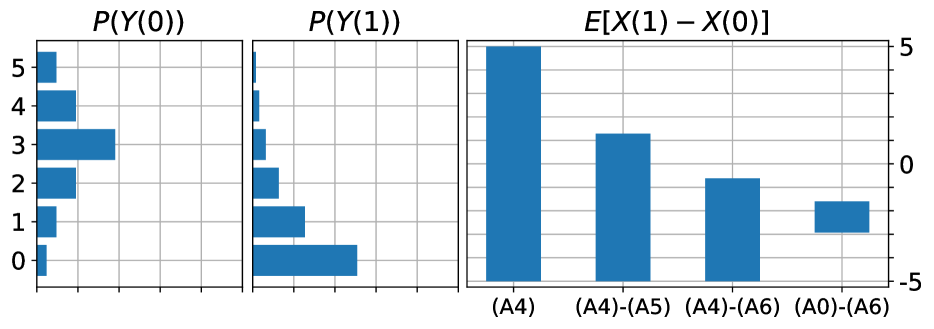
(a)

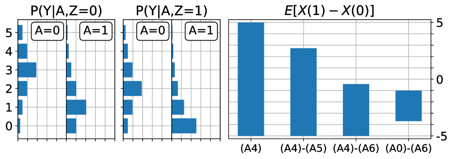
(b)

Figure 5: Bounds on the ATE $E[X(1)-X(0)]$ under different measurement error assumptions. (a) observed data distributions and bounds under in a randomized trial setting and (b) shows observed data distributions and bounds in an instrumental variable setting. Note that in the binary instrumental variable setting, $Z$ can be thought of as the assigned treatment and $A$ can be thought of as the observed treatment under partial compliance. $A=Z$ then corresponds to observed compliance and, in these cases ($A=Z=0$ and $A=Z=1$), the proxy distributions match the distributions in the randomized trial.

Application: Bounding the ATE in a randomized trial

To demonstrate computation of bounds for a causal parameter, we will now extend our previous examples to compute bounds on the ATE in a randomized trial where there is measurement error on the outcome variable. Assume that we are interested in the ATE of a binary treatment $A\in\{0,1\}$ on a variable $X$ using data from a single noisy proxy $Y$, with $X$ and $Y$ defined as before. We will assume the graphical model shown in Figure 2 (a) where $U$ represents an unobserved confounder. This model trivially satisfies the conditions of Proposition 1 and thus all graphical constraints can be expressed linearly. Figure 5 (a) shows the resulting bounds on the ATE as additional constraints are added. With only the graphical constraints, the bounds computed are the trivial bounds, though this will not be the case for all target parameters. Adding the causal assumptions (A4)-(A5), however, we are able to meaningfully bound the ATE away from zero. This bound becomes much tighter when the measurement error constraints are added. ∎

Application: Bounding the ATE in an instrumental variable model

Assume now that we are interested in the ATE of $A$ on $X$, but that $A$ is no longer randomized. Instead assume that we observe a binary instrumental variable $Z\in\{0,1\}$ and that all variables follow the graphical model shown in Figure 2 (c) where again $U$ represents an unobserved confounder. This model, which represents the IV model with measurement error on the outcome variable, similarly satisfies the conditions of Proposition 1 and we can again express all graphical constraints linearly. We assume that $P(A=0\mid Z=0)=P(A=1\mid Z=1)=0.8$ and $P(Y\mid A,Z)$ is distributed as shown in Figure 5 (b). These distributions were chosen to roughly simulate a trial with partial compliance where $Z$ represents treatment assignment and $A$ represents actual treatment. The resulting bounds on the ATE under different assumptions are also shown in Figure 5 (b). As expected, these bounds are wider than those produced in the randomize trial case, but the ATE can nevertheless be meaningfully bounded away from zero with only the causal assumptions (A4)-(A5). ∎

We re-emphasize that no known symbolic bounds exist for either of these settings and that the various numerical bounds in each setting were computed by simply making small changes to the implied LP. For a full description of the LPs in both of these cases, see Appendix E.

5 Related work

Measurement error occurs in many scientific settings and there is substantial literature on identification spread across a number of different methodological sub-disciplines. Much of this work concerns point identification in parametric models and we refer the interested reader to [6] and [13] for full treatments of these topics. In this section, we review several results on non-parametric partial identification in measurement error and related settings.

Several works, particularly in econometrics, have presented partial identifiability results under various measurement error models. [15] consider the setting presented in Section 2, deriving sharp bounds on the distribution of the ground truth under a particular error model where data is "contaminated" by data from another, unknown, distribution. [17] consider the same setting, presenting a procedure for verifying whether a particular distribution is in the identified set under a wide range of assumptions about the error distribution, including some non-linear assumptions. [14] consider partial identifiability in a class of finite mixture models which includes, as a special case, the Markov chain model considered in Proposition 3, similarly proposing a method for verifying if a distribution is in the identified set. Our work differs from [17] and [14] in that our methods do not require guess-and-check to calculate the complete identified set.

The optimization-based approach we use to derive sharp bounds is inspired by the approach used by [3] to derive sharp bounds on causal effects in trials with partial compliance. This approach was similarly applied by [16] to partially identify the ATE under measurement error on the treatment variable. This work is also related to efforts to enumerate constraints on margins of latent variable Bayesian Networks implied by the model [24, 10, 8]. In such works, unobserved variables are not of primary interest and do not have known cardinality, so no attempt is made to bound functionals of their distribution. However, as indicated by our use of results from [5], constraints on the observed data law can be used to derive restrictions on unobserved variables of known cardinality.

6 Discussion

In this work, we presented an approach for computing bounds on distributional and causal parameters involving a discrete variable which is subject to measurement error. At the heart of this approach is the encoding of the target parameter and modeling constraints as linear functions of the joint distribution of all variables in the model. The target parameter can then be maximized and minimized, with respect to this distribution and subject to the the modeling constraints, to produce sharp bounds for any observed data distribution. In particular, we provided a characterization of a class of graphical models that can be linearly expressed, and a procedure for finding a linear relaxation of models outside this class. We applied our approach to produce bounds under measurement error in settings with one or more proxies, including multiple important settings for which no known bounds currently exist.

Appendix A Proof of Proposition 3

Proof.

By assumption, $P(Y=1|X=0)\neq P(Y=0|X=0)$ and therefore

$$P(X=1)=\frac{P(Y=1)-P(Y=1|X=0)}{P(Y=1|X=1)-P(Y=1|X=0)}$$ (7)

We will derive sharp bounds on $P(X=1)$ by taking the union of the sharp bounds when $P(Y=1|X=0)>P(Y=0|X=0)$ and when $P(Y=1|X=0)<P(Y=0|X=0)$. The RHS of Equation 7 is continuous on each of these sub-regions, thus, as in the the linear programming case, we can find sharp bounds on each sub-region by finding the maximum and minimum of $P(X=1)$ on each sub-region subject to the modeling constraints. Consider first the case when $P(Y=1|X=0)>P(Y=0|X=0)$. For each value $a\in\mathcal{A}$ we have the following constraint which combines the observed data constraint and the conditional independence assumption $A\mathchoice{\mathrel{\hbox to0.0pt{$\displaystyle\perp$\hss}\mkern 2.0mu{\displaystyle\perp}}}{\mathrel{\hbox to0.0pt{$\textstyle\perp$\hss}\mkern 2.0mu{\textstyle\perp}}}{\mathrel{\hbox to0.0pt{$\scriptstyle\perp$\hss}\mkern 2.0mu{\scriptstyle\perp}}}{\mathrel{\hbox to0.0pt{$\scriptscriptstyle\perp$\hss}\mkern 2.0mu{\scriptscriptstyle\perp}}}Y|X$:

$$P(Y=1|A=a)= P(Y=1|X=0)(1-P(X=1|A=a))$$

$$+P(Y=1|X=0)P(X=1|A=a)$$

Let $q_{y|x}:=P(Y=y|X=x)$ and $\pi_{x|a}:=P(X=x|A=a)$. Then, using Equation 7, we can find the sharp upper bound for $P(X=1)$ on the $P(Y=1|X=0)>P(Y=0|X=0)$ sub-region by solving the following (non-linear) optimization problem:

$$\max_{q,\pi}\quad \frac{p_{1}-q_{1|0}}{q_{1|1}-q_{1|0}}$$

s.t. $$p_{1|a}=q_{1|0}(1-\pi_{1|a})+q_{1|1}\pi_{1|a}\,\,\,\forall a$$

$$q_{0|x}+q_{1|x}=1\,\,\,\forall x$$

$$\pi_{0|a}+\pi_{1|a}=1\,\,\,\forall a$$

$$0\leq q_{y|x},\pi_{x|a}\leq 1\,\,\,\forall y,x,a$$

To solve this optimization problem, we will fix $q_{1|1}$ and optimize with respect to $q_{1|0}$ and then optimize the resulting function with respect to $q_{1|1}$. That is, let

$$g(q_{1|1})=\max_{q_{1|0}}\quad \frac{p_{1}-q_{1|0}}{q_{1|1}-q_{1|0}}$$

s.t. $$p_{1|a}=q_{1|0}(1-\pi_{1|a})+q_{1|1}\pi_{1|a}\,\,\,\forall a$$

$$0\leq\pi_{1|a}\leq 1\,\,\,\forall a$$

$$0\leq q_{1|0}<q_{1|1}$$

In this case, all constraints are satisfied if and only if $0\leq q_{1|0}\leq\min_{a}p_{1|a}$ and the maximum is achieved when $q_{1|0}=0$. Thus, $g(q_{1|1})=\frac{p_{1}}{q_{1|1}}$. Next, we solve

$$\max_{q_{1|1}}\quad g(q_{1|1})=\frac{p_{1}}{q_{1|1}}$$

s.t. $$p_{1|a}=q_{1|1}\pi_{1|a}\,\,\,\forall a$$

$$0\leq\pi_{1|a}\leq 1\,\,\,\forall a$$

In this case, all constraints are satisfied if and only if $\max_{a}p_{1|a}\leq q_{1|1}\leq 1$ and the maximum value that satisfies this constraint is $\frac{p_{1}}{\max_{a}p_{1|a}}$. Applying similar reasoning to the minimization problem, we get a minimum value of $\frac{p_{1}-\min_{a}p_{1|a}}{1-\min_{a}p_{1|a}}$. Thus, when $q_{1|1}>q_{1|0}$, we have the following sharp bounds on $P(X=1)$

$$\frac{p_{1}-\min_{a}p_{1|a}}{1-\min_{a}p_{1|a}}\leq P(X=1)\leq\frac{p_{1}}{\max_{a}p_{1|a}}$$ (8)

Finally, we repeat this derivation for $q_{1|1}<q_{1|0}$ and take the union of these two sets of bounds to get the bounds in Proposition 3. The bounds for the $q_{1|1}<q_{1|0}$ are simply one minus the bounds for $q_{1|1}<q_{1|0}$ and thus the bounds for $P(X=1)$ are the same as the bounds for $P(X=0)$.

∎

Appendix B Combining Proposition 3 with Measurement Error Assumptions

In the presence of additional measurement error assumptions, the bounds in Proposition 3 can be further refined. In this section we present a few such refinements for measurement error assumptions (A1) and (A3) presented in Section 2 of the main paper as well as an additional non-linear assumption. (A2) does not apply to the binary case. All of these bounds can be derived with small modifications to the proof of Proposition 3.

Corollary 1.

If, in addition to the assumptions made in Proposition 3, we assume $P(Y=1|X=0)=0$ (i.e. (A1)), we have the following sharp bounds

$$P(X=1)\in\left[p_{1},\frac{p_{1}}{\max_{a}p_{1|a}}\right]$$

Corollary 2.

If, in addition to the assumptions made in Proposition 3, we assume $P(Y=0|X=0)>P(Y=1|X=0)$ (i.e. (A3)), we have the following sharp bounds

$$P(X=1)\in\left[\frac{p_{1}-\min_{a}p_{1|a}}{1-\min_{a}p_{1|a}},\frac{p_{1}}{\max_{a}p_{1|a}}\right]$$

Corollary 3.

If, in addition to the assumptions made in Proposition 3, we assume $P(Y=1|X=0)=P(Y=0|X=1)$ (i.e. label independent noise), we have the following sharp bounds

$$P(X=1)\in\left[p_{1},\frac{p_{1}-p^{*}}{1-2p^{*}}\right]\cup\left[1-\frac{p_{1}-p^{*}}{1-2p^{*}},1-p_{1}\right]$$

where $p^{*}=\min\left\{\min_{a}p_{1|a},1-\max_{a}p_{1|a}\right\}$.

Appendix C Proof of Proposition 2

Proof.

We first address the case in which an unobserved common parent is added. The factorization of the distribution over observed variables implied by $\mathcal{G}$ and by the DAG that results after the addition of the common parent, denoted $\mathcal{G}^{\prime}$ differ only in that the expression $P(A)P(B\mid pa_{\mathcal{G}}(B))$ in the former is replaced with $\int_{u}P(U)P(A\mid U)P(B\mid pa_{\mathcal{G}}(B),U)$. We now show that these expressions are equivalent.

$$\int_{u} P(U)P(A\mid U)P(B\mid pa_{\mathcal{G}}(B),U)$$

$$=\int_{u}P(U\mid pa_{\mathcal{G}}(B))P(A\mid U,pa_{\mathcal{G}}(B)\setminus\{A\})P(B\mid pa_{\mathcal{G}}(B),U)$$

$$=\int_{u}P(U,A,B\mid pa_{\mathcal{G}}(B)\setminus\{A\})$$

$$=P(A,B\mid pa_{\mathcal{G}}(B)\setminus\{A\})$$

$$=P(A\mid pa_{\mathcal{G}}(B)\setminus\{A\})P(B\mid pa_{\mathcal{G}}(B))$$

$$=P(A)P(B\mid pa_{\mathcal{G}}(B))$$

The first step is due $\{A,U\}\perp_{d}pa_{\mathcal{G}}(B)\setminus\{A\}$ in $\mathcal{G}^{\prime}$, because by construction $B$ is a collider on all paths between $\{A,U\}$ and $pa(B)\setminus\{A\}$. The second step is due to the chain rule of probabilities. The next two steps are a simple marginalization of $U$ and an expansion according to the chain rule, respectively. The final step is due again to $A\perp_{d}pa_{\mathcal{G}}(B)\setminus\{A\}$ in $\mathcal{G}^{\prime}$. This shows that after marginalization of the added common parent of $A$ and $B$, we recover exactly the model Markov to $\mathcal{G}$ over the variables in $\mathcal{G}$.

We now consider the scenario in which we add a common parent of $A$ and $B$, and remove the directed edge from $A$ to $B$. We denote the resulting DAG by $\mathcal{G}^{\prime\prime}$. The proof procedes very similarly; we show that $P(A)P(B\mid pa_{\mathcal{G}}(B))$ is equivalent to $\int_{u}P(U)P(A\mid U)P(B\mid pa_{\mathcal{G}}(B)\setminus\{A\},U)$. To do so, we note that $B\perp_{d}A\mid U,pa_{\mathcal{G}}(B)$ in $\mathcal{G}^{\prime\prime}$, as $A$ has no parents other than $U$, yielding

$$\int_{u} P(U)P(A\mid U)P(B\mid pa_{\mathcal{G}}(B)\setminus\{A\},U)$$

$$=\int_{u}P(U)P(A\mid U)P(B\mid pa_{\mathcal{G}}(B),U).$$

We can now procede exactly as before, concluding the proof. ∎

Appendix D Linear program for bounding $E[X]$ with two proxies

Below is the full linear program used for the application example in Section 3 of the main paper. The distribution $\psi$ is over the variables $\tilde{X}=\{X(a):a\in\mathcal{A}\}$ and $\tilde{Y}=\{Y(x):x\in\mathcal{X}\}$. This LP includes only the probability constraints and the observed data constraint and, as described in Section 3, the graphical constraints are implicitly enforced by $\psi$.

objective: $$\sum_{\tilde{x},\tilde{y}}(P(A=0)\tilde{x}_{0} \psi_{\tilde{x}\tilde{y}}+P(A=1)\tilde{x}_{1}\psi_{\tilde{x}\tilde{y}})$$ (9)

constraints: $$\sum_{\tilde{x},\tilde{y}}[\tilde{y}_{\tilde{x}_{0}}=y]\psi_{\tilde{x}\tilde{y}} =P(Y=y\mid A=0)$$

$$\sum_{\tilde{x},\tilde{y}}[\tilde{y}_{\tilde{x}_{1}}=y]\psi_{\tilde{x}\tilde{y}} =P(Y=y\mid A=1)$$

$$\psi_{\tilde{x}\tilde{y}} \geq 0$$

Appendix E Linear Program for Causal Bounds

First, we present the linear program used to bound the ATE in a randomized trial. As in the previous example, the distribution $\psi$ is over the variables $\tilde{X}=\{X(a):a\in\mathcal{A}\}$ and $\tilde{Y}=\{Y(x):x\in\mathcal{X}\}$. We include assumptions (A0), and (A2) through (A6), as described in the example given in Section 4 of the main paper. To obtain an LP corresponding to a subset of these assumptions, this LP can be modified by dropping constraints corresponding to assumptions not in that subset. Note that each of the constraints on measurement error are repeated twice - once to place restrictions on the relationship between $X(a)$ and $Y(a)$, and once for $X(a^{\prime})$ and $Y(a^{\prime})$. Then the ATE can be bounded by solving the LP in Figure 6.

objective: $$\sum_{\tilde{x},\tilde{y}}(\tilde{x}_{1}-\tilde{x}_{0})\psi_{\tilde{x}\tilde{y}}$$ (10)

constraints: $$\psi_{\tilde{x}\tilde{y}} \geq 0 \forall\,\tilde{x},\tilde{y}~{}~{}~{}~{}(PROB)$$

$$\sum_{\tilde{x},\tilde{y}}[\tilde{y}_{\tilde{x}_{a}}=y]\psi_{\tilde{x}\tilde{y}} =P(Y=y\mid A=a) \forall\,a,y~{}~{}~{}~{}(OBS)$$

$$\sum_{\tilde{x},\tilde{y}}[|\tilde{y}_{\tilde{x}_{a}}-\tilde{x}_{a}|>2]\psi_{\tilde{x}\tilde{y}} \leq\epsilon \forall\,a~{}~{}~{}~{}(A0)$$

$$\left|\sum_{\tilde{x},\tilde{y}}\psi_{\tilde{x}\tilde{y}}[\tilde{x}_{a}=x]([\tilde{y}_{\tilde{x}_{a}}=y]-[\tilde{y}_{\tilde{x}_{a}}=y^{\prime}])\right| \leq\lambda \forall\,a,|x-y|=|x-y^{\prime}|~{}~{}~{}~{}(A2)$$

$$\sum_{\tilde{x},\tilde{y}}\psi_{\tilde{x}\tilde{y}}[\tilde{x}_{a}=x]([\tilde{y}_{\tilde{x}_{a}}=y]-[\tilde{y}_{\tilde{x}_{a}}=y^{\prime}]) \geq 0 \forall\,a,|x-y|>|x-y^{\prime}|~{}~{}~{}~{}(A3)$$

$$\sum_{\tilde{x},\tilde{y}}\psi_{\tilde{x}\tilde{y}}[\tilde{x}_{1}<\tilde{x}_{0}] =0 (A5)$$

$$\sum_{\tilde{x},\tilde{y}}\psi_{\tilde{x}\tilde{y}}[\tilde{y}_{x}<\tilde{y}_{x^{\prime}}] =0 \forall x>x^{\prime}~{}~{}~{}~{}(A6)$$

Figure 6: LP for bounding the ATE in a randomized trial.

Next, we consider the LP used for bounding the ATE in the IV setting. We describe this LP in relation to the LP in Figure 6. In this case, $\psi$ is now also a distribution over $\tilde{A}=\{A(z):z\in\mathcal{Z}\}$. Then objective then becomes $\sum_{\tilde{a},\tilde{x},\tilde{y}}(\tilde{x}_{1}-\tilde{x}_{0})\psi_{\tilde{a}\tilde{x}\tilde{y}}$. The potential outcomes $A(z)$ and $A(z^{\prime})$ are similarly marginalized out of assumptions (A0), and (A2) through (A6). The only substantive change is that the observed data constraints must be modified as described in Section 4. This modification yields the following constraints

$$\sum_{\tilde{a},\tilde{x},\tilde{y}}\psi_{\tilde{a}\tilde{x}\tilde{y}}[\tilde{a}_{z}=a,\tilde{y}_{\tilde{x}_{a}}=y] =P(Y=y,A=a\mid Z=z) \forall\,z,a,y.$$

References

- [1] Roy Adams, Yuelong Ji, Xiaobin Wang, and Suchi Saria. Learning models from data with measurement error: Tackling underreporting. In International Conference on Machine Learning, pages 61–70, 2019.
- [2] Joshua D Angrist and Alan B Keueger. Does compulsory school attendance affect schooling and earnings? The Quarterly Journal of Economics, 106(4):979–1014, 1991.
- [3] Alexander Balke and Judea Pearl. Nonparametric bounds on causal effects from partial compliance data. Journal of the American Statistical Association, 1993.
- [4] Stan Becker, Kale Feyisetan, and Paulina Makinwa-Adebusoye. The effect of the sex of interviewers on the quality of data in a nigerian family planning questionnaire. Studies in Family Planning, pages 233–240, 1995.
- [5] Blai Bonet. Instrumentality tests revisited. In Jack S. Breese and Daphne Koller, editors, Proceedings of the 17th Conference on Uncertainty in Artificial Intelligence, pages 48–55. Morgan Kaufmann, 2001.
- [6] Raymond J Carroll, David Ruppert, Leonard A Stefanski, and Ciprian M Crainiceanu. Measurement error in nonlinear models: a modern perspective. CRC press, 2006.
- [7] Joseph A Catania, Diane Binson, Jesse Canchola, Lance M Pollack, Walter Hauck, and Thomas J Coates. Effects of interviewer gender, interviewer choice, and item wording on responses to questions concerning sexual behavior. Public Opinion Quarterly, 60(3):345–375, 1996.
- [8] R. J. Evans. Margins of discrete Bayesian networks. Annals of Statistics, 46(6A):2623–2656, 2018.
- [9] Robin Evans. Graphs for margins of bayesian networks. Scandinavian Journal of Statistics, 2016.
- [10] Robin J. Evans. Graphical methods for inequality constraints in marginalized dags, 2012.
- [11] Arthur Fine. Hidden variables, joint probability, and the bell inequalities. Physics Review Letters, 48, 1982.
- [12] D Gieger and Christopher Meek. Quantifier elimination for statistical problems. In Proceedings of the 15th Conference on Uncertainty in Artificial Intelligence, 1999.
- [13] Paul Gustafson. Measurement error and misclassification in statistics and epidemiology: impacts and Bayesian adjustments. CRC Press, 2003.
- [14] Marc Henry, Yuichi Kitamura, and Bernard Salanié. Partial identification of finite mixtures in econometric models. Quantitative Economics, 5(1):123–144, 2014.
- [15] Joel L. Horowitz and Charles F. Manski. Identification and robustness with contaminated and corrupted data. Econometrica, 63(2):281–302, 1995.
- [16] Kosuke Imai and Teppei Yamamoto. Causal inference with differential measurement error: Nonparametric identification and sensitivity analysis. American Journal of Political Science, 54(2):543–560, 2010.
- [17] Francesca Molinari. Partial identification of probability distributions with misclassified data. Journal of Econometrics, 144(1):81 – 117, 2008.
- [18] Panos M Pardalos and Stephen A Vavasis. Quadratic programming with one negative eigenvalue is np-hard. Journal of Global optimization, 1(1):15–22, 1991.
- [19] Judea Pearl. Causality. Cambridge University Press, 2009.
- [20] Davide Poderini, Rafael Chaves, Iris Agresti, Gonzalo Carvacho, and Fabio Sciarrino. Exclusivity graph approach to instrumental inequalities. In Uncertainty in Artificial Intelligence, pages 1274–1283. PMLR, 2020.
- [21] Kenneth J Rothman, Sander Greenland, and Timothy L Lash. Modern epidemiology. Lippincott Williams & Wilkins, 2008.
- [22] Shiv Shankar, Daniel Sheldon, Tao Sun, John Pickering, and Thomas G Dietterich. Three-quarter sibling regression for denoising observational data. In IJCAI, pages 5960–5966, 2019.
- [23] Péter Sólymos, Subhash Lele, and Erin Bayne. Conditional likelihood approach for analyzing single visit abundance survey data in the presence of zero inflation and detection error. Environmetrics, 23(2):197–205, 2012.
- [24] Elie Wolfe, Robert AW. Spekkens, and Tobias Fritz. The inflation technique for causal inference with latent variables. https://arxiv.org/abs/1609.00672, 2016.