Canonical translation surfaces for computing Veech groups

Abstract.

For each stratum of the space of translation surfaces, we introduce an infinite translation surface containing in an appropriate manner a copy of every translation surface of the stratum. Given a translation surface $(X,\omega)$ in the stratum, a matrix is in its Veech group $\mathrm{SL}(X,\omega)$ if and only if an associated affine automorphism of the infinite surface sends each of a finite set, the “marked” Voronoi staples, arising from orientation-paired segments appropriately perpendicular to Voronoi 1-cells, to another pair of orientation-paired “marked” segments.

We prove a result of independent interest. For each real $a\geq\sqrt{2}$ there is an explicit hyperbolic ball such that for any Fuchsian group trivially stabilizing $i$, the Dirichlet domain centered at $i$ of the group already agrees within the ball with the intersection of the hyperbolic half-planes determined by the group elements whose Frobenius norm is at most $a$.

Together, these results give rise to a new algorithm for computing Veech groups.

1. Introduction

Translation surfaces have been studied for decades, motivated by their appearance in various areas of mathematics, as well as by their intrinsic beauty. Although their study can be said to have begun with Teichmüller in the 1940s, it was work of Thurston in the 1970s and then Masur and Veech in especially the 1980s that brought this to the forefront. Results since that time have been numerous, with many further celebrated results.

1.1. Canonical surface per stratum

Any non-zero holomorphic 1-form $\omega$ on a closed Riemann surface $X$ gives local coordinates by integration, the result is a translation surface $(X,\omega)$, see say [M]. The zeros of $\omega$ result in singularities of the “flat” metric of the translation surface, the translation surfaces of the same set of orders of zeros form a stratum. Although in its natural topology, almost every stratum has more than one connected component [KZ], we associate to each stratum in a natural manner a single (infinite and, in general, non-connected) translation surface (see Definition 1) and show that every translation surface in the stratum can be appropriately represented on this canonical translation surface. More precisely, every translation surface of the stratum has an isometric copy of its Voronoi 2-cells on the canonical surface, allowing reconstruction of the original translation surface (see Proposition 7).

1.2. Veech groups

Various dynamical properties of the linear flow on a translation surface are determined by its Veech group, [V]. Every Veech group is a non-cocompact Fuchsian group [V]. By way of Teichmüller theory, when the group is a lattice, there is a corresponding algebraic curve in Riemann moduli space, $\mathcal{M}_{g}$ where $g$ is the genus of $X$, which is embedded with respect to the Teichmüller metric [V]; Veech named such curves Teichmüller curves, the translation surface is said to be a lattice surface. Veech also showed that certain triangle groups arise as what we call Veech groups, Bouw-Möller [BM] showed that up to finite index every non-cocompact Fuchsian triangle group so arises. On the other hand, almost every translation surface has a trivial Veech group [Mö]; and, whereas any polygon whose vertex angles are rational multiples of $\pi$ can be “unfolded” to achieve a translation surface, only three non-isosceles acute Euclidean triangles give lattice surfaces [KS, P]. Although constraints on which non-cocompact Fuchsian groups can be Veech groups, such as equality of trace field with invariant trace field if the group contains a hyperbolic element (essentially a result of [KS]) are known, a complete list of Fuchsian groups realized as Veech groups remains to be determined.

We give a new algorithm for computing Veech groups of translation surfaces (compact and without boundary), see §5.1. For a lattice surface, our algorithm completely computes the group. Our approach is different from the general algorithms in the literature [Bow] (see also [V2]), [BrJ, Mu, SmW] (implementations exist for the algorithms of Mukamel [Mu] and, as of quite recently by S. Freedman [F], of Bowman [Bow]), as well as from the special case algorithms [Sch, Fr]. As with most of these others, our algorithm has two parts: determining group elements and building a fundamental domain for the action of the group on the hyperbolic plane.

1.3. New criterion for membership in Veech group

To determine elements, we view a translation surface as being assembled from the disjoint union of its Voronoi 2-cells by identifying shared edges. There is a finite set of saddle connections whose images on the aforementioned canonical surface lead to a reconstruction of the original surface by identifying the two edges lying on the perpendicular bisector of the image of a saddle connection and that of its orientation-reversed saddle connection. We call these pairs of saddle connections Voronoi staples, and show that an element of $\mathrm{SL}_{2}(\mathbb{R})$ is in the Veech group exactly if it sends the Voronoi staples on the canonical surface to copies of orientation-paired saddle connections, Proposition 17.

1.4. New result on construction of Dirichlet domains

While we build a fundamental domain in a standard manner, we insist on finding elements in increasing Frobenius norm. We show a result of independent interest: For any Fuchsian group (trivially stabilizing $z=i$), the intersection of the half-planes determined by the elements of any explicitly bounded Frobenius norm agrees with the Dirichlet domain based at $z=i$ of the group within a corresponding explicit hyperbolic ball. See Proposition 25.

Recall that the Dirichlet domain is the nested (appropriately decreasing) limit of the convex bodies defined by intersecting the half-planes appropriately defined by finite sets of elements. Thus, the new result is that by taking the Frobenius norm ordering, there are also common domains which converge (appropriately increasing) to the interior of the Dirichlet domain. With this, we give a test for when the elements of a bounded Frobenius norm generate the group, see Theorem 26. This test thus gives a stopping condition for our algorithm, one that can only be fulfilled if the group is a lattice.

1.5. Examples, and related ongoing work

We have confirmed the computation of various Veech groups using the algorithm [Sa]. Here we use a simple example to illustrate matters (see Example 21, Figure 6, and Subsection 6.1). We also compute elements within an infinitely generated Veech group, finding that the first tens of thousands of elements in order of Frobenius norm are all contained in a subgroup generated by three elements (see Subsection 6.2 ).

In on-going work [Sa2], the second named author has shown how the approach of this paper can be reversed so as to begin with a Fuchsian group and determine those translation surfaces which have it as their Veech group.

This paper is based on the Ph.D. dissertation [E] of the first named author, as well as the implementation by the second named author [Sa]. That implementation was built upon Delecroix-Hooper’s “flat surface” computer code package [DH] written in SageMath [S].

2. Background

We introduce basic notation as well as remind the reader of some standard results.

2.1. Translation surfaces

See, say, [M, Mö, W] for much of the following.

2.1.1. Three views of a translation surface.

A translation surface is a real surface $X$ such that on the complement of a finite set of points $X\setminus\Sigma$ there is an atlas whose transition functions are all translations, and such that the flat structure on this complement extends to $X$ to have cone singularities of angles integral multiples of $2\pi$. Equivalently, a translation surface is a Riemann surface $X$ with a non-zero holomorphic differential (also called an abelian differential) $\omega$ where $\Sigma$ is the set of zeros of $\omega$; due to this view we often use the notation $(X,\omega)$ for a translation surface. A third equivalent form is as a collection of polygons in the Euclidean plane, with equal length parallel sides identified by translation (with the result an oriented surface); singularities occur only at points arising from vertices. We say $(X,\omega)$ in this form is polygonally presented.

It is common to change without warning from one to another of these perspectives when discussing any given translation surface. We will also use without warning the fact that subsurfaces of a translation surface are naturally translation surfaces.

Note that it is sometimes useful to allow the inclusion of removable singularities, thus points of cone angle $2\pi$, in $\Sigma$.

2.1.2. Affine diffeomorphisms and the Veech group

The group of translations of the plane is $\mathrm{Trans}(\mathbb{R}^{2})\cong\mathbb{R}^{2}$. A translation map between translation surfaces is a continuous map sending singularities to singularities which is a translation with respect to the local coordinates given by the respective translation atlases. Recall that the affine group of the plane is $\mathrm{Trans}(\mathbb{R}^{2})\rtimes\mathrm{GL}_{2}(\mathbb{R})$. An affine diffeomorphism of a translation surface is a homeomorphism $f:X\to X$ which sends $\Sigma$ to itself, while inducing an affine diffeomorphism on $X\setminus\Sigma$. That is, the maps on local coordinates (as induced in the usual manner) are elements of the affine group of the plane. Under composition, the set of all of these forms a group, $\mathrm{Aff}(X,\omega)$. Because of the normality of translations in the affine group of the plane, the linear part of each affine diffeomorphism $f$ is constant, independent of choice of local coordinates, and thus there is a group homomorphism $\mathrm{der}:\mathrm{Aff}(X,\omega)\to\mathrm{GL}_{2}(\mathbb{R})$. The image of the subgroup of orientation-preserving affine diffeomorphisms, $\mathrm{Aff}^{+}(X,\omega)$, is called the Veech group of $(X,\omega)$. We denote the kernel of $\mathrm{der}$ by $\mathrm{Trans}(X,\omega)$.

Convention. Unless otherwise stated, the notation $(X,\omega)$ will denote a closed translation surface: compact without boundary.

The flat structure on any translation surface allows Lebesgue measure on the plane to induce a measure on the surface. When the translation surface is compact this is a finite measure, and it is an observation of Veech [V] that the Veech group is then a subgroup of $\mathrm{SL}_{2}(\mathbb{R})$. To emphasize this, one denotes the Veech group by $\mathrm{SL}(X,\omega)$. Veech [V] also showed that $\mathrm{SL}(X,\omega)$ is a discrete subgroup of $\mathrm{SL}_{2}(\mathbb{R})$.

2.1.3. Saddle connections, strata, matrix group action

It is easy to see that the foliation of $\mathbb{R}^{2}$ by horizontal lines induces a foliation on $X\setminus\Sigma$. The lines of this foliation meet at points of $\Sigma$ of cone angle greater than $2\pi$ to give saddle singularities.

Any geodesic ray emanating from a singularity is called a separatrix. A separatrix joining two singularities (with no other singularity in its interior) is called a saddle connection, or simply as in [KS] a segment. Integration along a segment results in the corresponding element of $\mathbb{C}$, called a holonomy vector.

The collection of all (closed) translation surfaces $(X,\omega)$ with the holomorphic 1-form $\omega$ having zeros of orders $d_{1},\dots,d_{s}$ (with repetition allowed) is called a stratum and denoted $\mathcal{H}(d_{1},\dots,d_{s})$. Note that the cone angle at a zero of order $d$ is $2(d+1)\pi$. By either the Riemann-Roch Theorem or that of Gauss-Bonnet, all translation surfaces of a fixed stratum have the same genus.

The group $\mathrm{GL}_{2}(\mathbb{R})$ acts on the collection of all translation surfaces by way of post-composition with local coordinate functions. This action preserves each stratum. In the setting of closed translation surfaces, Veech showed that the $\mathrm{SL}_{2}(\mathbb{R})$-stabilizer of $(X,\omega)$ under this action is isomorphic to $\mathrm{SL}(X,\omega)$. Furthermore, for any $M\in\mathrm{SL}_{2}(\mathbb{R})$, one has $M\mathrm{SL}(X,\omega)M^{-1}=\mathrm{SL}(M\cdot(X,\omega)\,)$.

2.1.4. Voronoi decomposition

Each translation surface has a flat metric with conical singularities on it. Masur-Smillie [MS] sketch the theory of Voronoi decompositions subordinate to the set of singularities. A Voronoi 2-cell is an open, connected, set of points which are closer to some singularity than to any other. The boundary of each Voronoi 2-cell is a union of Voronoi 1-cells consisting of open geodesics (each of whose points have exactly two distinct shortest paths to $\Sigma$), meeting in Voronoi 0-cells (single points each having at least three distinct shortest paths to $\Sigma$). Each compact $(X,\omega)$ is the union of finitely many open Voronoi 2-cells (exactly one per each element of $\Sigma$), finitely many Voronoi 1-cells and finitely many Voronoi 0-cells. We will refer to the union of a Voronoi 1-cell and its two endpoint 0-cells simply as an edge.

3. Canonical surface, Voronoi staples and a Veech group membership criterion

3.1. Canonical translation surface, $\mathcal{O}$

To each stratum we associate an infinite translation surface.

Definition 1.

Given a stratum $\mathcal{H}(d_{1},\dots,d_{s})$, for each subscript $i$ let $\mathcal{O}_{i}$ be the infinite translation surface $(\mathbb{C},z^{d_{i}}\,dz)$ and let $\mathcal{O}=\mathcal{O}(d_{1},\dots,d_{s})$ be the disjoint union of the $\mathcal{O}_{i}$.

Partition the index set $\{1,\dots,s\}$ corresponding to repeated values of the $d_{i}$, with partition elements of cardinalities say $n_{1},\dots,n_{t}$.

Lemma 2.

Each $\mathrm{Trans}(\mathcal{O}_{i})$ is a cyclic group of order $1+d_{i}$, whose generator acts as a rotation of angle $2\pi$. The group $\mathrm{Trans}(\mathcal{O})$ is generated by the product of permutation groups $S_{n_{1}}\times\cdots\times S_{n_{t}}$ acting by change of index, along with the direct product of the various $\mathrm{Trans}(\mathcal{O}_{i})$.

Proof.

Any element of $\mathrm{Trans}(\mathcal{O}_{i})$ maps the singularity to itself and off of this induces translations in local coordinates. These local coordinates arise from the ramified covering $\mathcal{O}_{i}\to\mathbb{C}$ and thus any induced translation is in fact the identity. In other words, $\mathrm{Trans}(\mathcal{O}_{i})$ restricts to $\mathcal{O}_{i}\setminus\{0\}$ to be the deck transformation group of the covering of the punctured complex plane. Thus, $\mathrm{Trans}(\mathcal{O}_{i})$ is indeed a cyclic group of order $1+d_{i}$, generated by a rotation of $2\pi$.

Acting by permutation of indices, $S_{n_{1}}\times\cdots\times S_{n_{t}}$ certainly gives a subgroup of $\mathrm{Trans}(\mathcal{O})$. Furthermore, the trivial extension to $\mathcal{O}$ of the action of $\mathrm{Trans}(\mathcal{O}_{i})$, acting as the identity on all other $\mathcal{O}_{j}$, gives an injection of $\mathrm{Trans}(\mathcal{O}_{i})$ into $\mathrm{Trans}(\mathcal{O})$. Any affine diffeomorphism $\varphi$ of $\mathcal{O}$ must preserve cone angles, and hence composition with some element of $S_{n_{1}}\times\cdots\times S_{n_{t}}$ gives an affine diffeomorphism that sends each $\mathcal{O}_{i}$ to itself. If furthermore $\varphi\in\mathrm{Trans}(\mathcal{O})$ then so is this composition, and hence for each $i$ it restricts to give an element of $\mathrm{Trans}(\mathcal{O}_{i})$. Thus, the result holds. ∎

Lemma 3.

For each $A\in\mathrm{GL}_{2}\mathbb{R}$ there is an affine diffeomorphism $f_{A}\in\mathrm{Aff}(\mathcal{O})$ such that $\mathrm{der}(f_{A})=A$.

Proof.

We first briefly sketch the result in the setting of $(\mathbb{C},dz)$, see Figure 1. The surface $A\cdot(\mathbb{C},dz)$ is formed by post-composing the chart maps of $(\mathbb{C},dz)$ with $A$, using the standard action of $\mathrm{GL}_{2}\mathbb{R}$ on $\mathbb{C}\cong\mathbb{R}^{2}$. The identity map on $\mathbb{C}$ gives $\mathrm{Id_{\mathbb{C}}}:(\mathbb{C},dz)\to A\cdot(\mathbb{C},dz)$, of Jacobian equal to $A$. Similarly, the map sending points of $\mathbb{C}\cong\mathbb{R}^{2}$ to their corresponding image under $A$ induces a diffeomorphism $F_{A}:A\cdot(\mathbb{C},dz)\to(\mathbb{C},dz)$ of Jacobian equal to $I_{2}$, the identity matrix. Thus the composition $F_{A}\circ\mathrm{Id_{\mathbb{C}}}$ is an affine diffeomorphism whose Jacobian equals $A$.

Figure 1. Local coordinate calculation shows that $F_{A}\circ\mathrm{Id_{\mathbb{C}}}$ has Jacobian $A$. The similarly defined map $f_{A}:\mathcal{O}\to\mathcal{O}$ is also of linear part $A$.

The above shows that whenever $\mathcal{O}_{i}$ corresponds to a removable singularity, there is an affine diffeomorphism of it, say $f_{i}$, whose linear part is $A$. Now, for any other index $i$, we have $\mathrm{Id_{\mathcal{O}_{i}}}:\mathcal{O}_{i}\to A\cdot\mathcal{O}_{i}$ of linear part $A$. Furthermore, similar to $F_{A}$ above, we have $\widehat{F}_{A,i}:A\cdot\mathcal{O}_{i}\to\mathcal{O}_{i}$ of trivial linear part. Letting $\widehat{F}_{A}:A\cdot\mathcal{O}\to\mathcal{O}$ be the map which restricts to $\widehat{F}_{A,i}$ on each $A\cdot\mathcal{O}_{i}$, one finds that $f_{A}=\widehat{F}_{A}\circ\mathrm{Id_{\mathcal{O}}}$ is a homeomorphism taking singularities to singularities and whose linear part is $A$. ∎

The locally length-minimizing paths on $\mathcal{O}$ are easily described.

Lemma 4.

For each $\mathcal{O}_{i}$, any two distinct points are connected by a unique geodesic. Each such geodesic is either a straight line segment, or a connected sequence of such segments meeting at the singularity with (minimum) angle at least $\pi$.

Proof.

The description of the geodesics is a special case of Strebel’s result for an arbitrary (half-)translation surface $(Y,\alpha)$, see Theorem 8.1 of [Str]. Since $\mathcal{O}_{i}$ is simply connected, any two points of $\mathcal{O}_{i}$ are connected by a unique geodesic (see [Str] Theorem 14.2.2 and Corollary 18.2). ∎

Lemma 5.

Suppose that $(X,\omega)$ is an element of $\mathcal{H}(d_{1},\dots,d_{s})$. Then there is an injective translation map of the disjoint union of the open Voronoi 2-cells of $(X,\omega)$ into $\mathcal{O}$. This map is unique, up to the action of $\mathrm{Trans}(\mathcal{O})$ on the image.

Proof.

Enumerate the elements of $\Sigma$ so that for each $i$, $\sigma_{i}\in\Sigma$ has cone angle $2(1+d_{i})\pi$. Fix $i$ and for typographic ease let $\sigma=\sigma_{i}$, and let $\mathcal{C}_{\sigma}$ be the Voronoi 2-cell centered at $\sigma$.

We can choose and fix a horizontal ray from the origin of $\mathcal{O}_{i}$ to measure angles from, and define a generalized system of polar coordinates in the obvious fashion. That is, every point other than the origin of $\mathcal{O}_{i}$ is uniquely represented by an ordered pair of positive real number and angle between $0$ and $2(d_{i}+1)\pi$.

We introduce a similar generalized polar coordinate system in $\mathcal{C}_{\sigma}$. By definition, the open set $\mathcal{C}_{\sigma}$ contains no other singularity, hence it contains some singular coordinate patch about $\sigma$. By shrinking as necessary, this coordinate patch is a totally ramified covering of some disk centered at the origin of $\mathbb{C}$, of degree $d_{i}+1$. In this patch we can choose a lift of a ray along the positive $x$-axis and identify each point other than $\sigma$ by an ordered pair of positive real number and angle between $0$ and $2(d_{i}+1)\pi$. Since each point of $\mathcal{C}_{\sigma}$ is connected to $\sigma$ by a unique shortest path and these paths vary continuously in $\mathcal{C}_{\sigma}$, we can extend the polar coordinates to all of $\mathcal{C}_{\sigma}$. The injective map $\iota_{\sigma}:\mathcal{C}_{\sigma}\to\mathcal{O}_{i}$ sending a point to the corresponding point with the same polar coordinates is then easily seen to be a translation map.

Now we let $\sigma=\sigma_{i}$ vary and define a map from the disjoint union of the Voronoi 2-cells to $\mathcal{O}$ to be given by applying the appropriate $\iota_{\sigma}$. This is certainly an injective translation map. Given another such translation map, we can compose with an element of $S_{n_{1}}\times\cdots\times S_{n_{t}}$ to ensure that both send the Voronoi 2-cell of $\sigma_{i}$ to $\mathcal{O}_{i}$ for each $i$. The only remaining freedom is accounted for by the action of each $\mathrm{Trans}(\mathcal{O}_{i})$. The result thus holds. ∎

3.2. Recovering $(X,\omega)$

We give some details of the reconstruction of $(X,\omega)$ from the collection of the images on the canonical surface of the Voronoi 2-cells.

We fix some notation.

Definition 6.

We will assume throughout that some injective translation map $\iota$ as above of the union of the Voronoi 2-cells of $(X,\omega)$ into $\mathcal{O}$ has been fixed. For each singularity $\sigma$ we let $\mathcal{O}_{\sigma}=\mathcal{O}_{i}$ where $\iota$ sends $\sigma$ to the origin of $\mathcal{O}_{i}$. As in the previous proof, we also let $\mathcal{C}_{\sigma}$ be the Voronoi 2-cell centered at $\sigma$ and $\iota_{\sigma}:\mathcal{C}_{\sigma}\to\mathcal{O}_{\sigma}$ the corresponding translation map. Unless otherwise stated, $0$ will denote the singularity of $\mathcal{O}_{\sigma}$.

Recall that $(X,\omega)$ is isometric to the quotient space of the disjoint union of the closure of its Voronoi cells under the relation defined by the identification of shared edges. Similarly, each $\iota(\mathcal{C}_{\sigma})$ has a collection of line segments comprising its closure which can be identified so as to recover $(X,\omega)$. Note that for each $\sigma$, we have $\overline{\iota(\mathcal{C}_{\sigma})}=\overline{\iota_{\sigma}(\mathcal{C}_{\sigma})}$.

Proposition 7.

Let $Y$ be the disjoint union of the various $\overline{\iota(\mathcal{C}_{\sigma})}$. For each $\sigma$ any edge of $\mathcal{C}_{\sigma}$ can be uniquely identified with a line segment in $\overline{\iota(\mathcal{C}_{\sigma})}$ so that the two line segments corresponding to a common edge of Voronoi 2-cells are translation equivalent and such that the resulting equivalence relation on $Y$ results in a quotient metric space that is isometric to $(X,\omega)$.

Proof.

Fix $\sigma$ and choose any edge $e$ of $\mathcal{C}_{\sigma}$ as well as a point $p$ in the interior of $e$. The polar coordinates of $\mathcal{C}_{\sigma}$ extend to give local coordinates in some sufficiently small neighborhood of this regular point. Since the inverse function $j$ taking $\iota(\mathcal{C}_{\sigma})$ to $\mathcal{C}_{\sigma}$ is given by identifying points of the same polar coordinates, it extends linearly to include all of this neighborhood in its image. Suppose that $e$ is shared with $\mathcal{C}_{\sigma^{\prime}}$ and let $j^{\prime}$ be the inverse function in this setting. Polar coordinates here also give local coordinates in some sufficiently small common neighborhood $U$ of $p$. These two local coordinates on $U\subset(X,\omega)$ differ by a translation, from which it follows that $j^{-1}(U)$ is a translation equivalent copy of $(j^{\prime})^{-1}(U)$ in $\mathcal{O}_{\sigma}$.

Figure 2 is related to the following construction. Let $\hat{U}$ be the set taken by $j$ to $U$ and let $\hat{p}\in\hat{U}$ be the preimage of $p$. There is a unique shortest path from $\sigma$ to the regular point $p\in(X,\omega)$. Correspondingly there is a radial line from $0$ to $\hat{p}$. As we vary $p\in U$ (while remaining in the interior of $e$), the radial lines vary continuously. We have the analogous situation with respect to the shortest paths from $\sigma^{\prime}$. The translation equivalence can thus be extended to the set comprised of the radial lines in $\mathcal{C}_{\sigma^{\prime}}$ (the lines translating ‘rigidly’ with their endpoints). Note that $\sigma^{\prime}$ is sent to some regular point, say $w\in\mathcal{O}_{\sigma}$. As well, each of our $\hat{p}$ has equal length straight line segments to $0$ and to $w$. It follows that the set of these $\hat{p}$ is a line segment on the perpendicular bisector $L$ of the line segment joining $0$ and $w$.

Varying $p$ shows that $j$ can be extended so that all of the interior of $e$ has a well defined $j$-preimage, and that this preimage lies on $L$ and by continuity we find that $j$ sends a line segment $\hat{e}$ on the boundary of $\overline{\iota(\mathcal{C}_{\sigma})}$ to $e$, and that all of $\hat{e}$ lies on $L$. It also follows that $\hat{e}$ and the subset of the closure of $\iota_{\sigma^{\prime}}(\mathcal{C}_{\sigma^{\prime}})$ corresponding to $e$ are translation equivalent. Thus, the announced equivalence relation exists, and the quotient space of $Y$ is indeed isometric to $(X,\omega)$. ∎

When $\sigma$ is fixed we will continue to use $\hat{p}$ and $\hat{e}$ to denote the preimage of a point $p$ and of an edge $e$ respectively, under the extension $j$ of the inverse of $\iota_{\sigma}$. We also introduce another bit of notation.

Figure 2. Construction for Proposition 7, $\iota$-images of a common edge of two Voronoi 2-cells can be identified by a translation equivalence. Here $\hat{p}$ is an interior point of a boundary edge $\hat{e}$ of $\iota(\mathcal{C}_{\sigma})$, $0$ denotes the origin of $\mathcal{O}_{\sigma}$, $\hat{U}$ is a neighborhood of $\hat{p}$, $w$ is the reflection of $0$ through the line of $\hat{e}$. Black lines outline a triangle in the closure of $\iota(\mathcal{C}_{\sigma})$. Blue dotted lines give the equal length segments joining $\hat{p}$ to $0$ to $w$.

Definition 8.

For $z\in\mathcal{O}_{\sigma}\setminus\{0\}$, let $D(z)$ be the open disk of center $z$ and radius equal to the distance from $0$ to $z$.

Figure 3. Voronoi 0-cell $q$ corresponds to an endpoint $\hat{q}$ of a boundary line segment $\hat{e}$ of $\overline{\iota(\mathcal{C}_{\sigma})}\subset\mathcal{O}_{\sigma}$. The proof of Proposition 7 shows that a reflection of the triangle $T$ through the line of $\hat{e}$ is translation equivalent to a triangle within a paired Voronoi 2-cell. Proposition 9 shows that the disk $D(\hat{q})$ is covered by translation equivalent copies of triangles in the $n+2$ (counted with possible repetition) Voronoi 2-cells on whose boundaries $q$ lies; pictured: $n=2$. The points $w,w_{1},\dots,w_{n}$ are the resulting images of the singularities. The dashed blue arc with the black dotted arc form the boundary of $D(\hat{q})$, inside the disk is the sector $S_{-}$ (not labeled in figure). The disk lies in the union of that sector and the sector $S^{+}$ (outer arc dotted in red) of the disk about the other end of $\hat{e}$.

Proposition 9.

Suppose that $e$ is an edge of $\mathcal{C}_{\sigma}$ and that $p\in e$. Then $D(\hat{p})$ is contained in the union of a finite number of triangles in $\mathcal{O}_{\sigma}$, each of which is translation equivalent to a triangle whose vertices are the singularity and endpoints of one edge of the 2-cell of some Voronoi 2-cell of $(X,\omega)$. In particular, the inverse $j$ to $\iota_{\sigma}$ extends so as to take $D(\hat{p})$ to an open set of $(X,\omega)\setminus\Sigma$.

Proof.

We begin by showing that the initial result holds for the endpoints of $e$. Normalize so that $\hat{e}$ is vertical and denote its lowest point by $\hat{q}$, see Figure 3. Let $r$ be the distance from $\hat{q}$ to $0$. Now, $\iota(\mathcal{C}_{\sigma})$ includes (the interior of) the triangle $T$ whose vertices are $0$ and the endpoints of $\hat{e}$. The proof of Proposition 7 shows that the reflection of $T$ through $\hat{e}$, say $T^{\prime}$, is translation equivalent to a triangle inside $\iota(\mathcal{C}_{\sigma^{\prime}})$. As in that proof, let $w$ be the reflection of $0$ through the line of $\hat{e}$. Let $S_{-}$ be the lower sector of $D(\hat{q})$ bounded by the radial lines ending at $0$ and $w$. We aim to show that $S_{-}$ is contained in an appropriate union of triangles.

Corresponding to $\hat{q}$ is an endpoint of $e$ say, $q$. There is a finite number of additional Voronoi 2-cells, say $\mathcal{C}_{\sigma_{1}},\dots,\mathcal{C}_{\sigma_{n}}$ (repetition allowed) such that $q$ is an endpoint of an edge of each; enumerate so that the corresponding edges are $e_{1},\dots,e_{n+1}$ where $e_{1}$ is shared by $\mathcal{C}_{\sigma}$ and $\mathcal{C}_{\sigma_{1}}$, $e_{n+1}$ is a shared edge of $\mathcal{C}_{\sigma_{n}},\mathcal{C}_{\sigma^{\prime}}$ and any other $e_{i}$ is shared by $\mathcal{C}_{\sigma_{i-1}},\mathcal{C}_{\sigma_{i}}$. Since $q$ is a regular point, the polar coordinates of $\mathcal{O}_{\sigma}$ allow the extension of the inverse map $j$ to include a neighborhood of $\hat{q}$. As well, the directions of the various edges as given by geodesic segments emanating from $q$ are well defined. This allows us to repeatedly use the construction of the proof of Proposition 7. Thus, for each $i$, we can translate the $\iota$-copy of a triangle within $\iota(\mathcal{C}_{\sigma_{i}})$ so that the vertices of the closure on $\mathcal{O}_{\sigma}$ are $\hat{q}$, the second endpoint of a line segment $\hat{e}_{i}$, and a point $w_{i}$ on the boundary arc of $S_{-}\,$. In particular, there is an open neighborhood of $\hat{q}$ contained in the union of all of the triangles on $\mathcal{O}_{\sigma}$.

If $S_{-}$ is not already contained in the union of these triangles, then let $\hat{q}_{i}$ be the lower endpoints of the $\hat{e}_{i}$. These also correspond to regular points, and thus there are translates of closures of $\iota$-images of triangles which meet at them. Note that the reflections involved place the images of the corresponding singularities outside of $S_{-}\,$. (Alternatively: These images must be external to $S_{-}$, as if not then there is a straight path from $\hat{q}$ to such an image that gives rise to a path from $q$ to $\Sigma$ that is shorter than the radius of $S_{-}$, a contradiction.) We can now continue this process, finding translated images of triangles so as to share edges, with singularities of images always external to $S_{-}\,$. By the compactness of $(X,\omega)$ there are finitely many edges of Voronoi 2-cells, and thus the triangles must have area bounded below by a positive constant. Therefore, allowing for ever more generations, we must eventually have $S_{-}$ included in the union of a finite number of our triangles on $\mathcal{O}_{\sigma}$.

We can now argue with the other endpoint of $\hat{e}$ instead of $\hat{q}$. Let $R$ be the distance from this point to $0$ and let $S^{+}$ be the sector of center this second point and radius $R$ which is bounded by the radial lines to $0$ and to $w$. By the arguments above $S^{+}$ is similarly covered by triangles. By Euclidean geometry, $r\leq R+|\hat{e}|$ (where $|\cdot|$ denotes length). It follows that the disk $D(\hat{q})$ is contained in the union of $S_{-}$ and $S^{+}$. By symmetry, the disk of the other endpoint is also contained in the union of these sectors. But, similar comparisons of lengths of paths show that $D(\hat{p})\subset S_{-}\cup S^{+}$ also holds for points $\hat{p}$ lying in the interior of $\hat{e}$.

Finally, since none of the images of the singularities of the various triangles lies in $S_{-}\cup S^{+}$, given $\hat{p}$ the map $j$ extends so as to send $D(\hat{p})$ to an open subset of $(X,\omega)\setminus\Sigma$. ∎

3.3. Closed Voronoi 2-cells as convex bodies on $\mathcal{O}$

We define key notions for the following.

Definition 10.

Any separatrix $\rho$ emanating from $\sigma$ is such that the map $\iota$ sends $\rho\cap\mathcal{C}_{\sigma}$ to a line segment emanating from the origin of $\mathcal{O}_{\sigma}$. Let $\breve{\rho}$ be the open ray formed by stopping $\rho$ at the first singularity it encounters thereafter, if any such exists. The linear continuation of $\iota(\,\rho\cap\mathcal{C}_{\sigma}\,)$ whose length agrees with that of $\breve{\rho}$ then gives the unique isometric embedding of $\breve{\rho}$ into $\mathcal{O}$ agreeing with $\iota$ restricted to $\mathcal{C}_{\sigma}$. We denote this image by $\hat{\iota}(\rho)$.

Given a saddle connection $s$, we call $\hat{\iota}(s)$ a marked segment for $(X,\omega)$.

Definition 11.

Given a saddle connection $s$, let $\sigma$ be the initial endpoint of $s$. We define $\hat{s}$ to be the terminal endpoint of $\hat{\iota}(s)$. We also define the half-space of $s$ to be

$$H_{\iota}(s)=\{z\in\mathcal{O}_{\sigma}\mid d(0,z)\leq d(z,\hat{s})\},$$

where $d(\cdot,\cdot)$ denotes the distance on $\mathcal{O}_{\sigma}$ and (for simplicity’s sake) $0$ denotes its origin, $\iota(\sigma)$.

Proposition 12.

Given a saddle connection $s$ emanating from a singularity $\sigma$, let $s^{\perp}$ denote the perpendicular bisector of $\hat{\iota}(s)$. Then $s^{\perp}$ is the boundary of $H_{\iota}(s)$.

Proof.

Away from its origin, $\mathcal{O}_{\sigma}$ has a Euclidean metric, and thus $s^{\perp}$ is indeed well-defined. Similarly, in the case that $\sigma$ is a removable singularity the result is well known from elementary geometry.

In all other cases, we invoke Strebel’s description of geodesics, Lemma 4 above. Given two points other than the origin, if the radial segments having these points as endpoints are of angle less than $\pi$, then the geodesic between them is simply the straight line segment connecting them in a single coordinate chart. If their angle is greater than $\pi$, then the geodesic is the union of two radial line segments.

Now, if $\hat{\iota}(s)$ makes an angle greater than or equal to $\pi$ with the ray from the origin to $z\in\mathcal{O}_{\sigma}$, then $d(z,\hat{s})=d(z,0)+d(0,\hat{s})$ and certainly $z\notin\partial H_{\iota}(s)$. All other $z$ lie within an angle of $\pi$ on either side of $\hat{\iota}(s)$. The ramified covering $\mathcal{O}_{\sigma}\to\mathbb{C}$ sends each sector of angle $\pi$ isometrically to $\mathbb{C}$, and the result then follows from the classical case. ∎

Definition 13.

For a singularity $\sigma$ we define the convex body of $\sigma$ to be

$$\Omega_{\sigma}=\cap_{s}\,H_{\iota}(s)\,,$$

where $s$ runs through the set of saddle connections emanating from $\sigma$.

Naturally enough, we say that a subset of any $\mathcal{O}_{i}$ is convex if it contains the straight line segment joining any two of its points.

Proposition 14.

We have equality of sets

$$\Omega_{\sigma}=\overline{\iota(\mathcal{C}_{\sigma})}.$$

Furthermore, to each edge $e$ of $\mathcal{C}_{\sigma}$ is associated a saddle connection $s$ emanating from $\sigma$ such that the image of $e$ in $\overline{\iota(\mathcal{C}_{\sigma})}$ lies on $s^{\perp}$. Letting $\mathcal{E}_{\sigma}^{\perp}$ denote the collection of all such saddle connections,

$$\Omega_{\sigma}=\cap_{s\in\mathcal{E}_{\sigma}^{\perp}}\,H_{\iota}(s).$$

Proof.

We first show that $\overline{\iota(\mathcal{C}_{\sigma})}=\cap_{s\in\mathcal{E}_{\sigma}^{\perp}}\,H_{\iota}(s)$. Choose an edge $e$ of $C_{\sigma}$, and let $\sigma^{\prime}$ be the singularity whose Voronoi 2-cell shares this edge. Let $\hat{e}$ in $\overline{\iota(\mathcal{C}_{\sigma})}$ correspond to $e$ as above. For $\hat{q}$ either endpoint of $\hat{e}$ by Proposition 9, the polar coordinates inverse map $j$ extends to have domain including the open disk $D(\hat{q})$, which it takes to a set of regular points of $(X,\omega)$. With $w$ as above, the straight line from $0$ to $w$ has its interior contained in $D(\hat{q})$ (for at least one of the choices of $\hat{q}$) and since $j$ extends continuously to take $w$ to $\sigma^{\prime}$, there is a corresponding saddle connection $s$ on $(X,\omega)$ connecting $\sigma$ to $\sigma^{\prime}$ and such that $\hat{s}=w$. Therefore, $\hat{e}$ is in $s^{\perp}$. From this it follows that $\overline{\iota(\mathcal{C}_{\sigma})}=\cap_{s\in\mathcal{E}_{\sigma}^{\perp}}\,H_{\iota}(s)$.

Certainly $\cap_{s\in\mathcal{E}_{\sigma}^{\perp}}\,H_{\iota}(s)\supset\Omega_{\sigma}$. If the two convex sets were not equal then there would be some $s$ such that $s^{\perp}$ meets $\iota(\mathcal{C}_{\sigma})$ and in particular there must be some endpoint $\hat{q}$ of an edge $\hat{e}$ that is closer to $\hat{s}$ than to $0$. But then $\hat{s}\in D(\hat{q})$. From the proof of Proposition 9, $D(\hat{q})\subset S\cup S^{+}$ and since $0$ is on the boundary of this union, the line segment from $0$ to $\hat{s}$ is contained in the closure of $S\cup S^{+}$. Similarly to in the previous paragraph, $s$ is the image under the extension of $j$ of the line segment. However, this shows that the point $q$ corresponding to $\hat{q}$ is closer to $\Sigma$ than is $\hat{q}$ to $0$, a contradiction. Thus, no such $s$ can exist. ∎

3.4. Voronoi staples determine $(X,\omega)$

We introduce several key sets for our considerations.

Definition 15.

Reversing orientation on any saddle connection $s$ of $(X,\omega)$ results in a saddle connection $s^{\prime}$. We say that $s,s^{\prime}$ are orientation-paired, and denote the set of these pairs by $\mathcal{M}(X,\omega)$. We then call $\hat{\iota}(s),\hat{\iota}(s^{\prime})$ orientation-paired marked segments, and denote the set of these pairs by $\widehat{\mathcal{M}}(X,\omega)$. When $s\in\mathcal{E}_{\sigma}^{\perp}$, let $e$ denote the edge of $\mathcal{C}_{\sigma}$ lying on its perpendicular bisector, and $e^{\prime}$ be $e$ with the opposite orientation. Letting $\sigma^{\prime}$ denote the singularity from which $s^{\prime}$ emanates, $e^{\prime}$ is an edge of $\mathcal{C}_{\sigma^{\prime}}$, from which it follows that $s^{\prime}\in\mathcal{E}_{\sigma^{\prime}}^{\perp}\,$. We then call $\{s,s^{\prime}\}$ a Voronoi staple, and denote the set of all Voronoi staples by $\mathcal{S}(X,\omega)$. The corresponding subset of $\widehat{\mathcal{M}}(X,\omega)$ is called the marked Voronoi staples, denoted by $\widehat{\mathcal{S}}(X,\omega)$, see Figure 4.

Figure 4. Left: Two distinct 2-cells comprising the Voronoi decomposition of the hexagonal torus subordinate to two removable singularities. Right: The resulting image of the cells under $\iota$ as well as of the saddle connections under $\hat{\iota}$. The marked Voronoi staples — $\{a,a^{\prime}\},\{b,b^{\prime}\},\{c,c^{\prime}\}$ — show how to glue together the closure of the images of the 2-cells to obtain the surface.

Our choice of terminology is to highlight the implication of Propositions  7 and 14: $(X,\omega)$ can be viewed as the disjoint union of the closures of the various $\Omega_{\sigma}$ “stapled together” by identifying sides lying on perpendicular bisectors of members of the same marked Voronoi staple.

Theorem 16.

Suppose that both $(X_{1},\omega_{1}),(X_{2},\omega_{2})$ belong to $\mathcal{H}(d_{1},\dots,d_{s})$ and choose maps $\iota_{1},\iota_{2}$ to $\mathcal{O}$. Then $(X_{1},\omega_{1}),(X_{2},\omega_{2})$ are equivalent translation surfaces if and only if $\widehat{\mathcal{S}}(X_{1},\omega_{1})$ and $\widehat{\mathcal{S}}(X_{2},\omega_{2})$ are in the same $\mathrm{Trans}(\mathcal{O})$-orbit.

Proof.

First suppose that there is an element of $\mathrm{Trans}(\mathcal{O})$ taking $\hat{\iota}_{2}(\,\mathcal{S}(X_{2},\omega_{2})\,)$ to $\hat{\iota}_{1}(\,\mathcal{S}(X_{1},\omega_{1})\,)$. We can replace $\iota_{2}$ by its composition with this map and assume equality of these images. Proposition 14 then shows that for each singularity $\sigma_{1}$ of $(X_{1},\omega_{1})$ there is a singularity $\sigma_{2}$ of $(X_{2},\omega_{2})$ so that $\Omega_{\sigma_{1}}=\Omega_{\sigma_{2}}$. Furthermore, since each identification of corresponding pairs of sides of the various $\Omega_{\sigma_{1}},\Omega_{\sigma^{\prime}_{1}}$ is indexed by some Voronoi pair, we find also that the $\Omega_{\sigma_{2}},\Omega_{\sigma^{\prime}_{2}}$ are identically paired. Therefore, the resulting surfaces are isometric and in particular translation equivalent. Proposition 7 then gives that $(X_{1},\omega_{1}),(X_{2},\omega_{2})$ are translation equivalent.

If $(X_{1},\omega_{1}),(X_{2},\omega_{2})$ are equivalent translation surfaces, then there is a homeomorphism $f:(X_{2},\omega_{2})\to(X_{1},\omega_{1})$ that is, off of singularities, a translation in local coordinates. In particular, $f$ maps Voronoi 2-cells to Voronoi 2-cells and sends $\mathcal{S}(X_{2},\omega_{2})$ to $\mathcal{S}(X_{1},\omega_{1})$. The composition $\iota_{1}\circ f$ then restricts to a translation map of the Voronoi 2-cells of $(X_{2},\omega_{2})$ into $\mathcal{O}$; by Lemma 5 there is an element of $\mathrm{Trans}(\mathcal{O})$ which composed with $\iota_{2}$ equals $\iota_{1}\circ f$ on the Voronoi 2-cells of $(X_{2},\omega_{2})$. Equality holds then also for the extended maps, and thus $\widehat{\mathcal{S}}(X_{1},\omega_{1})$ (the image of the first) is in the $\mathrm{Trans}(\mathcal{O})$ -orbit of $\widehat{\mathcal{S}}(X_{2},\omega_{2})$. ∎

3.5. Membership criterion

The next result applies the above with $(X_{1},\omega_{1})=(X,\omega)$ and $(X_{2},\omega_{2})=A\cdot(X,\omega)$ to give a criterion for $A$’s membership in $\mathrm{SL}(X,\omega)$. For this, we use the map $f_{A}:\mathcal{O}\to\mathcal{O}$ of Lemma 3.

Proposition 17 (Membership Criterion, initial form).

Fix $(X,\omega)$ and suppose $A\in\mathrm{SL}_{2}\mathbb{R}$. Then $A\in\mathrm{SL}(X,\omega)$ if and only if $f_{A}$ sends $\widehat{\mathcal{S}}(X,\omega)$ to a subset of $\widehat{\mathcal{M}}(X,\omega)$, up to some element of $\mathrm{Trans}(\mathcal{O})$.

Proof.

We first establish an intermediate result for all $A\in\mathrm{SL}_{2}\mathbb{R}$, confer Figure 5. For any $A\in\mathrm{SL}_{2}\mathbb{R}$, let $\hat{\iota}_{A}$ be the (unique up to translations) analog of $\iota$ for $A\cdot(X,\omega)$. The map $\mathrm{Id}_{X}:A\cdot(X,\omega)\to(X,\omega)$ has linear part $A^{-1}$, and sends the orientation-paired saddle connections of $A\cdot(X,\omega)$ set-wise to those of $(X,\omega)$. Hence $\hat{\iota}\circ\mathrm{Id}_{X}$ sends these to $\widehat{\mathcal{M}}(X,\omega)$. Composing further with $\mathrm{Id}_{\mathcal{O}}:{\mathcal{O}}\to A\cdot{\mathcal{O}}$ (whose linear part is $A$) gives that the orientation-paired saddle connections of $A\cdot(X,\omega)$ are sent isometrically in pairs into $A\cdot\mathcal{O}$ by $\mathrm{Id}_{\mathcal{O}}\circ\hat{\iota}\circ\mathrm{Id}_{X}$. Thereafter composing with $\widehat{F}_{A}$ sends these isometrically into $\mathcal{O}$. Since $f_{A}=\widehat{F}_{A}\circ\mathrm{Id}_{\mathcal{O}}$, Lemma 5 (arguing by the density of directions of saddle connections) shows that $f_{A}\circ\hat{\iota}\circ\mathrm{Id}_{X}$ is $\hat{\iota}_{A}$, up to $\mathrm{Trans}(\mathcal{O})$-equivalence. Thus, we may assume equality and hence that $\hat{\iota}_{A}$ sends the orientation-paired saddle connections of $A\cdot(X,\omega)$ isometrically to $f_{A}(\,\widehat{\mathcal{M}}(X,\omega)\,)$.

Figure 5. Up to an element of $\mathrm{Trans}(\mathcal{O})$, $\hat{\iota}_{A}$ sends $\mathcal{M}(\,A\cdot(X,\omega)\,)$ to $f_{A}(\,\widehat{\mathcal{M}}(X,\omega)\,)$.

($\Rightarrow$) Given $A\in\mathrm{SL}(X,\omega)$, then also $A^{-1}\in\mathrm{SL}(X,\omega)$. By Theorem 16, we may assume that $\hat{\iota}(\,\mathcal{S}(X,\omega)\,)$ and $\hat{\iota}_{A^{-1}}(\,\mathcal{S}(\,A^{-1}\cdot(X,\omega)\,)\,)$ are equal. From the previous paragraph, this is a subset of $f_{A^{-1}}(\,\widehat{\mathcal{M}}(X,\omega)\,)$. It follows that $f_{A}\circ\hat{\iota}(\,\mathcal{S}(X,\omega)\,)$ equals some subset of $\widehat{\mathcal{M}}(X,\omega)$. This first direction hence holds.

($\Leftarrow$) Again since $\mathrm{SL}(X,\omega)$ is a group, it suffices to show that $A\in\mathrm{SL}(X,\omega)$ if $f_{A^{-1}}(\,\widehat{\mathcal{S}}(X,\omega)\,)\subset\widehat{\mathcal{M}}(X,\omega)$. To show this, we apply $f_{A}$ and find $\widehat{\mathcal{S}}(X,\omega)\subset f_{A}(\,\widehat{\mathcal{M}}(X,\omega)\,)=\widehat{\mathcal{M}}(\,A\cdot(X,\omega)\,)$. Any singularity $\sigma$ of $A\cdot(X,\omega)$ is identified with a fixed singularity of $(X,\omega)$, naturally also denoted by $\sigma$. Since $\Omega_{\sigma}(\,A\cdot(X,\omega)\,)$ is the intersection of the half-spaces for all marked segments associated to $\sigma$, the convex body given by the intersection over the $s\in\mathcal{E}_{\sigma}^{\perp}(X,\omega)$ contains $\Omega_{\sigma}(\,A\cdot(X,\omega)\,)$. By Proposition 14, this larger convex body is $\Omega_{\sigma}(X,\omega)$, and is a copy of the closure of the Voronoi 2-cell for $\sigma$ on $(X,\omega)$.

Summing over all $\sigma$ shows the natural Lebesgue measure of $A\cdot(X,\omega)$ is at most the measure of $(X,\omega)$. However, since $A\in\mathrm{SL}_{2}\mathbb{R}$, the measure of $A\cdot(X,\omega)$ is the same as that of $(X,\omega)$. Therefore, equality of convex bodies holds for each $\sigma$. We now apply the construction of Proposition 7 to each of the collections of $\Omega_{\sigma}(\,A\cdot(X,\omega)\,)$ and $\Omega_{\sigma}(X,\omega)$. The fact that $f_{A}$ respects orientation-pairings assures that the resulting two translation surfaces are equivalent. Therefore, $A\cdot(X,\omega)$ and $(X,\omega)$ are translation equivalent and hence $A\in\mathrm{SL}(X,\omega)$. ∎

Remark 18.

In his Ph.D. dissertation [E], Edwards shows that the $\mathrm{SL}_{2}\mathbb{R}$ action on $\mathcal{O}$ induces an action on $\mathrm{Trans}(\mathcal{O})$-equivalent classes of $\mathbb{Z}_{2}$-paired subsets of $\mathcal{O}$, and that the stabilizer of the class of $\widehat{\mathcal{M}}(X,\omega)$ is exactly $\mathrm{SL}(X,\omega)$.

For ease, let us say that the length of a Voronoi staple is the length of the underlying saddle connection (with one of the possible orientations). In the following, we assume that some $\iota:(X,\omega)\to\mathcal{O}$ has been chosen. Recall that the maximum singular value of a real matrix $A$ is the maximum of length of the image of unit vectors under $A$ and thus gives a bound on how much $A$ can expand lengths.

Definition 19.

For each positive real number $r$, let $\mathcal{P}_{r}=\mathcal{P}_{r}(X,\omega)$ be the set of orientation pairs of marked segments of length at most $r$.

Corollary 20 (Membership Criterion, with bounds).

Let $\ell$ be the maximal length of any Voronoi staple of $(X,\omega)$. Suppose that $\nu\in[1,\infty)$ and $A\in\mathrm{SL}_{2}\mathbb{R}$ has maximum singular value at most $\nu$.

Then $A\in\mathrm{SL}(X,\omega)$ if and only if $f_{A}$ maps the set of marked Voronoi staples of $(X,\omega)$ into some $\mathrm{Trans}(\mathcal{O})$-translate of $\mathcal{P}_{\nu\ell}$.

Sketch.

We use Proposition 17. Since $f_{A}$ has linear part $A$, it expands lengths by at most the maximum singular value of $A$ and hence the image of any marked Voronoi staple can have length at most $\nu\ell$. ∎

Example 21 (Respecting orientation-pairing is crucial).

It is important to note that an element $A\in\mathrm{SL}_{2}(\mathbb{R})$ may take marked segments to marked segments, but still fail the membership criterion, due to it not respecting orientation-pairings. Figure 6 illustrates this in the case of an $(X,\omega)\in\mathcal{H}(2)$, formed by glueing three unit squares together in the configuration shown and identifying opposite sides, where $A=\left(\begin{smallmatrix}1&0\\ 1&1\end{smallmatrix}\right)$ sends the horizontal marked segment $s$ to the marked segment $\gamma$, but does not send the paired $s^{\prime}$ to $\gamma^{\prime}$. Nor is there any element of $\mathrm{Trans}(\mathcal{O})$ that can resolve this. However, the reader may wish to verify that $B=\left(\begin{smallmatrix}1&0\\ 2&1\end{smallmatrix}\right)$ does fulfill the membership criterion.

Figure 6. Illustrating Example 21. Left: Surface formed by identifying opposite sides, each segment is of length one, is in $\mathcal{H}(2)$. Voronoi partition indicated in black, dashed. Angle measurement beginning at horizontal of left middle vertex (first $2\pi$ in single blue, second in double brown, third in triple black rings). Right: The single connected component of $\mathcal{O}$, also of singularity of angle $6\pi$, represented as three copies of $\mathbb{C}$ glued along the positive $x$-axis in cyclic order left to right. Red arrows show one marked Voronoi staple $\{s,s^{\prime}\}$. Black arrows show one choice, up to action of $\mathrm{Trans}(\mathcal{O})$, for $\gamma=f_{A}(s)$ and its orientation paired marked segment, where $A=\left(\begin{smallmatrix}1&0\\ 1&1\end{smallmatrix}\right)$. Blue arrow is $f_{A}(s^{\prime})$. Since $\gamma^{\prime}\neq f_{A}(s^{\prime})$ (and similarly for all $\mathrm{Trans}(\mathcal{O})$-images of $\gamma$), $A$ fails the membership criterion. Also indicated: dots give endpoints of other marked segments, shaded disks are of radius $\nu\ell$ with $\ell,\nu$ defined as in Corollary 20, of values here $\ell=1$ and $\nu=\nu(\,||A||)=\sqrt{(3+\sqrt{5})/2}$, see Definition 22.

4. Nesting hyperbolic polygons agreeing on ever larger balls

The previous section presents theoretical results for determining elements of a specific discrete subgroup of $\mathrm{SL}_{2}\mathbb{R}$. Here we give results on using finite lists of elements of any given Fuchsian group $\Gamma\subset\mathrm{PSL}_{2}(\mathbb{R})$ to determine aspects of a fundamental domain for the action of $\Gamma$ on the Poincaré upper half-plane model of hyperbolic space, $\mathbb{H}$. Recycling notation, in this section we use $H,\Omega$ to again indicate half-spaces and their intersections, but in the context of the $\mathbb{H}$.

Convention. Throughout this section, we assume that $\Gamma$ has no non-trivial elements fixing $i\in\mathbb{H}$.

(Should in fact such elements exist, then since $\Gamma$ acts properly discontinuously, conjugating this group by a sufficiently small translation must result in a group whose stabilizer of $i$ is trivial. This was used to determine the translation surface underlying the computations for Figure 7.)

The standard construction of the Dirichlet domain (centered at $z=i$) for a group $\Gamma$ respecting our convention is algorithmic: one takes the intersection of half-planes one at a time, see [K] for a textbook discussion. We thus contemplate taking the intersection of such half-planes for all elements of Frobenius norm of at most a given bound. As the bound goes to infinity, these convex bodies nest down to the Dirichlet domain for $\Gamma$.

However, more is true. We show that as the Frobenius norm increases there are ever larger hyperbolic balls within which these convex bodies already match the Dirichlet domain of the full group. This allows us to use an area computation to detect if $\Gamma$ is generated by the elements whose norm is bounded by any explicit constant.

4.1. Bounded Frobenius norm elements give Dirichlet domain within bounded ball

Let $d_{\mathbb{H}}(z,w)$ denote the standard hyperbolic distance between two points in the upper half-plane. For $A\in\mathrm{SL}_{2}\mathbb{R}$ let $||A||$ denote the Frobenius norm of $A$, that is $||A||=\sqrt{\mathrm{tr}(A^{t}A)}$. It is well-known that the Frobenius norm of $A$ equals the square-root of the sum of the squares of the singular values of $A$. Note also that the Frobenius norm descends to give a well-defined function on $\mathrm{PSL}_{2}\mathbb{R}$, which we also call the Frobenius norm.

Definition 22.

Define the function

$$\nu:[\sqrt{2},\infty) \to[1,\infty)$$

$$a \mapsto\sqrt{\dfrac{1}{2}(a^{2}+\sqrt{a^{4}-4}\,)}\,.$$

Note that $\nu(||A||)$ gives the maximum singular value of $A$.

The next result is presumably well-known but we do not know of a source where it is explicitly stated.

Lemma 23.

Suppose that $A\in\mathrm{SL}_{2}\mathbb{R}\setminus\mathrm{SO}_{2}\mathbb{R}$. Then the hyperbolic distance from $i$ to $A\cdot i$ is given by

$$d_{\mathbb{H}}(i,A\cdot i)=2\log\nu(\,||A||\,).$$

In particular, the hyperbolic ball centered at $i$ and of radius $r=\log\nu(\,||A||\,)$ is contained in the half-plane of elements that are nearer to $i$ than to $A\cdot i$,

$$H_{i}(A)\supset B(i,\log\nu(\,||A||\,)).$$

Definition 24.

For any positive real number $a$, let $\Gamma^{a}$ denote the set of all elements of $\Gamma$ whose Frobenius norm is at most $a$. Furthermore, for any subset $S\subset\Gamma$, let $\Omega(\,S\,)=\cap_{A\in S}\,H_{i}(A)$. Thus when $S$ is a subgroup of $\Gamma$, we have that $\Omega(\,S\,)$ is its Dirichlet domain centered at $z=i$.

The very construction of Dirichlet domains shows that as $a$ increases, the $\Omega(\,\Gamma^{a}\,)$ nest down to $\Omega(\,\Gamma\,)$. Since $a\mapsto\log\nu(a)$ defines an increasing function, the following shows that within ever growing balls the $\Omega(\,\Gamma^{a}\,)$ fully describe $\Omega(\,\Gamma\,)$. (Of course, neither must be completely contained in any such fixed ball.)

Proposition 25.

For each $a\geq\sqrt{2}$,

$$\Omega(\,\Gamma\,)\cap B(i,\log\nu(a))=\Omega(\,\Gamma^{a}\,)\cap B(i,\log\nu(a)\,).$$

Proof.

Since $a\mapsto\log\nu(a)$ is a strictly increasing function, Lemma 23 implies that also if $a<||A||$ then $H_{i}(A)$ contains the ball $B(i,\log\nu(\,a\,))$. Since $\Omega(\,\Gamma\,)$ is formed from $\Omega(\,\Gamma^{a}\,)$ by intersection with all such $H_{i}(A)$, with $A\in\Gamma$, the result holds. ∎

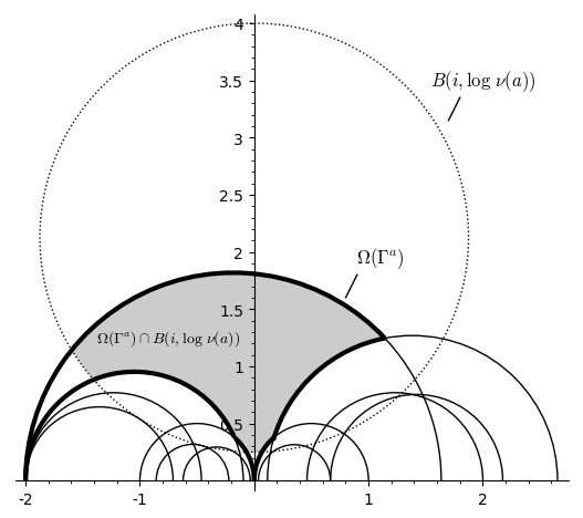
Figure 7. The shaded region shows where the computed intersection of half-planes from elements of small Frobenius norm must agree with the Dirichlet region of the full group, as guaranteed by Proposition 25. Here, $\Gamma=\mathrm{SL}(M\cdot(X,\omega))$, where $(X,\omega)$ is given in Example  21, see also Figure 6, and $M=\left(\begin{smallmatrix}1&0\\ 1/2&1\end{smallmatrix}\right)$ is used to obtain a surface whose Veech group has trivial stabilizer of $z=i$. Here $a=\sqrt{257}/4$.

4.2. Recognizing a generating set

This subsection gives a theoretical result that leads to a stopping condition for our algorithm to compute $\mathrm{SL}(X,\omega)$, when this group is a lattice.

Theorem 26.

Suppose that $a\geq\sqrt{2}$ is such that

$$\mu_{{}_{\mathbb{H}}}(\,\Omega(\Gamma^{a}\,)\,)<2\,\mu_{{}_{\mathbb{H}}}(\,\Omega(\,\Gamma^{a}\,)\cap B(i,\log\nu(a)\,)\,).$$

Then the subset $\Gamma^{a}$ generates $\Gamma$. In particular, $\Gamma$ is a lattice.

Proof.

Since $\Gamma$ is a discrete group, the subset $\Gamma^{a}$ is finite and hence $\Omega(\,\Gamma^{a}\,)$ has finitely many sides. By construction there is a finite subset of $\Gamma^{a}$ pairing these sides. Let $G$ be the subgroup of $\Gamma$ generated by these side parings. Then

$$\mu_{{}_{\mathbb{H}}}(\Omega(G))\leq\mu_{{}_{\mathbb{H}}}(\Omega(\Gamma^{a})).$$

Proposition 25 combines with this to give

$$\mu_{{}_{\mathbb{H}}}(\Omega(\Gamma)) \geq\mu_{{}_{\mathbb{H}}}(\,\Omega(\,\Gamma\,)\cap B(i,\log\nu(a))\,)$$

$$=\mu_{{}_{\mathbb{H}}}(\,\Omega(\,\Gamma^{a}\,)\cap B(i,\log\nu(a))\,)$$

$$>\frac{1}{2}\mu_{{}_{\mathbb{H}}}(\Omega(\,\Gamma^{a})\,)$$

$$\geq\frac{1}{2}\mu_{{}_{\mathbb{H}}}(\,\Omega(G)\,).$$

Hence, the index of $G$ in the group $\Gamma$ is

$$|\Gamma:G|=\frac{\mu_{{}_{\mathbb{H}}}(\Omega(G))}{\mu_{{}_{\mathbb{H}}}(\Omega(\Gamma))}<2.$$

Therefore, $G=\Gamma$. It follows that $\Gamma^{a}$ generates $\Gamma$.

The initial hypothesis implies that $\mu_{{}_{\mathbb{H}}}(\,\Omega(\,\Gamma^{a}\,)\,)$ is finite. We deduce that $\Gamma$ is finitely generated and has finite co-volume. It is a lattice. ∎

5. From theory to algorithm

We sketch how the results above can be combined to give an algorithm to compute Veech groups.

5.1. Basic steps of algorithm

Given a polygonal presentation of $(X,\omega)$, one can calculate to find a Voronoi decomposition. Further calculation leads to the Voronoi staples, as one can explicitly calculate all saddle connections up to any given length. Thus, the set $\widehat{\mathcal{S}}(X,\omega)$ and the value $\ell$ of Corollary 20 are knowable with finite calculation.

We test membership using Corollary 20. We can form candidate matrices by choosing of the saddle connections of two distinct saddle connections and a choice of image vectors. Beginning with $a=\sqrt{2}$, we choose image vectors from the holonomy vectors corresponding to elements of $\mathcal{P}_{\nu(a)\,\ell}$. We then check whether the candidate matrix $A$ is such that $f_{A}$ does send the marked Voronoi staples pairwise into orientation-paired marked segments, up to an element of $\mathrm{Trans}(\mathcal{O})$. Exactly when this is the case is $A\in\mathrm{SL}(X,\omega)$. We complete this round for all possible candidate matrices for this value of $a$. We then form $\Omega(\Gamma^{a})$ and apply the obvious test implied by Theorem 26. If this test is positive, then we have determined all of what is rightly denoted as $\mathrm{PSL}(X,\omega)$. (The only other way that our algorithm halts is by a user-entered upper bound on the Frobenius norm of elements to test.) Otherwise, we increase $a$ (say by doubling its value).

5.2. Some technical details

We roughly indicate how some of the technical matters of implementing the algorithm are addressed.

• From $\mathrm{PSL}(X,\omega)$ to $\mathrm{SL}(X,\omega)$. Passing from $\mathrm{PSL}(X,\omega)$ to $\mathrm{SL}(X,\omega)$ is merely a matter of determining if $-I_{2}\in\mathrm{SL}(X,\omega)$. Since $||-I_{2}||=\sqrt{2}$, this is directly tested using Corollary 20.

• Finding a Veech group that trivially stabilizes $z=i$. The stabilizer inside of all of $\mathrm{SL}_{2}(\mathbb{R})$ of $z=i$ is $\mathrm{SO}_{2}(\mathbb{R})$, from which a Fuchsian group $\Gamma$ follows our convention exactly if $\Gamma^{\sqrt{2}}\cap\mathrm{SO}_{2}(\mathbb{R})\subset\{\pm I_{2}\}$. Given a translation surface $(X,\omega)$, we test for this by calculating $\mathrm{PSL}(X,\omega)^{\sqrt{2}}$. Upon failure, we rather find an $M$ such that $M\cdot(X,\omega)$ trivially stabilizes $z=i$ and compute $\mathrm{SL}(M\cdot(X,\omega)\,)$ with the algorithm as already sketched; thereafter, conjugating by $M^{-1}$ gives $\mathrm{SL}(X,\omega)$. (Figure 7 arises from a computation in such a setting.) It is the fact that $\mathrm{SL}(X,\omega)$ is discrete and hence that $\mathrm{PSL}(X,\omega)$ acts properly discontinuously on $\mathbb{H}$ (in particular, fixed points are isolated), that implies the existence of some such $M$. In fact, there is some $n\in\mathbb{N}$ such that $M=\left(\begin{smallmatrix}1&0\\ 1/n&1\end{smallmatrix}\right)$ suffices. (An iterative loop can determine the smallest value of $n$ for which this holds.)

  
  

• “Marked” data from $(X,\omega)$. Values of the map $\hat{\iota}$ to $\mathcal{O}$ are represented in terms of data structures reflecting the geometry of $(X,\omega)$: We first choose an enumeration of the singularities; as illustrated in Figure 6, for each singularity we choose one of the horizontal rays emanating from it, and measure angles beginning at that marked horizontal. (The difference of choices of the horizontal is accounted for by $\mathrm{Trans}(\mathcal{O}_{i})$ as in Lemma 2.) Thereafter, each saddle connection is recorded as a vector in the plane, along with a record of the singularity from which it emanates, as well as of which multiple of $2\pi$ gives the copy of $\mathbb{C}$ in which its image lies (compare Figure 6), and finally the record includes a pointer to its orientation-paired saddle connection.

• $\mathrm{SL}_{2}(\mathbb{R})$ action on marked segments. When applying the membership criterion, it is crucial that one notes that for $A\in\mathrm{SL}_{2}(\mathbb{R})$, $f_{A}$ can send a marked segment from one copy of $\mathbb{C}$ into one of the neighboring $\mathbb{C}$. This is a matter of the vector being “pushed” across the positive $x$-axis. As an example, the reader can verify that in the setting of Example 21 and Figure 6 $f_{A}$ sends $1-i/2$ in the first copy of $\mathbb{C}$ into the second copy of $\mathbb{C}$.

6. Verified calculations

We have verified the results of running code based upon this algorithm for a collection of surfaces. These include various “L” surfaces, particular (double) regular polygons, the famed “eierliegende Wollmilchsau” surface, and others, see [Sa] for most of these.

6.1. An “L”-surface

Here we content ourselves with a brief report on the calculation of the main running example of this paper. For the translation surface $(X,\omega)$ of Example 21 and Figure 6, applying the algorithm, we found that $\mathrm{SL}(X,\omega)$ is generated by the matrices

$$S=\begin{pmatrix}0&-1\\ 1&0\end{pmatrix},\,A=\begin{pmatrix}2&1\\ -1&0\end{pmatrix}.$$

Note that $S$ squares to give $-I_{2}$ and that $SA$ is equal to $B=\big{(}\begin{smallmatrix}1&0\\ 2&1\end{smallmatrix}\big{)}$ (confer the final sentence of Example 21 ). We can easily recognize that the ideal triangle of vertices at $-1,0,\infty$ is a fundamental domain for this group: $S$ sends the $y$-axis to itself (fixing $z=i$) and $A$ sends the geodesic of “feet” $-1$ and $0$ to the vertical line through $x=-1$. Thus $\mathrm{PSL}(X,\omega)$ is a Fuchsian triangle group, of signature $(0;2,\infty,\infty)$ — it is of genus zero, has two cusps and one orbifold point of index $2$. The fundamental domain has area $\pi$, and $\mathrm{SL}(X,\omega)$ is certainly a subgroup of $\mathrm{SL}_{2}(\mathbb{R})$; our calculation thus accords with the first entry in the table of results in Section 4.2 of [Sch] (the “L”-surface there is translation equivalent to our $(X,\omega)$ ).

Note that with $M$ as in the caption of Figure 7, $M^{-1}$ sends the Dirichlet domain centered at $z=i$ for $\mathrm{PSL}(M\cdot(X,\omega)\,)$ suggested in that figure to the Dirichlet domain at $z=M^{-1}\cdot i$ for $\mathrm{PSL}(X,\omega)$. This image is a pentagon with ideal vertices at $-1,0$; the sides meeting at $-1$ are paired by $A$, those meeting at $0$ by $B$, the remaining side passes through $z=i$ and is paired with itself by $S$.

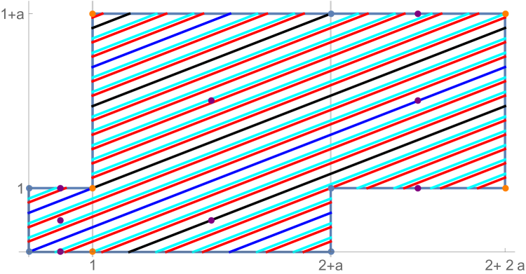
Figure 8. Cylinder composition in a parabolic direction not in $\langle P_{1},P_{2}\rangle$ for McMullen’s $a=1+\sqrt{3}$ example of infinitely generated Veech group. Here $P_{1},P_{2}$ are parabolic elements corresponding to the vertical and horizontal directions. The surface, formed by identifying opposite facing sides, is in $\mathcal{H}(1,1)$. Marked points are the vertices, which give rise to the cone singularities, and the Weierstrass points, see [Mc].

6.2. Investigating an infinitely generated Veech group

McMullen [Mc] gave an infinite family of translation surfaces in $\mathcal{H}(1,1)$, each of whose Veech group is infinitely generated (an “infinitely generated” group is one which cannot be finitely generated). Our algorithm can of course find elements in order of Frobenius norm for such groups; we investigated $\mathrm{SL}(X,\omega)$ for his surface corresponding to $a=1+\sqrt{3}$, see Figure 8 (and the figures in [Mc]). Each of the vertical and the horizontal directions of this surface determine respective parabolic elements $P_{1}=\begin{pmatrix}1&0\\ 1&1\end{pmatrix},P_{2}=\begin{pmatrix}1&2+a\\ 0&1\end{pmatrix}\in\mathrm{SL}(X,\omega)$. Intriguingly enough, we found that all of the $25,010$ elements of $\mathrm{SL}(X,\omega)$ up to Frobenius norm 256 lie in the subgroup generated by $-I_{2}$ and the parabolic elements $P_{1}$ and $P_{2}$.

This leads us to ask for the study of the general growth behavior in terms of $x$ of the minimal number of elements within an infinitely generated group to generate the subgroup containing all elements of Frobenius norm up to $x$.

In the meantime, we give an explicit element of $\mathrm{SL}(X,\omega)\setminus\langle-I_{2},P_{1},P_{2}\rangle$. The Dirichlet domain of the Fuchsian $\langle P_{1},P_{2}\rangle$ based at $z=i$ is easily seen to have vertical sides at $x=\pm(2+a)/2$ as well as sides whose feet at infinity are $-2,0$ and $0,2$ and free sides $(-(2+a)/2,-2)$ and $(2,(2+a)/2)$. By Theorem 9.2 of [Mc], any direction of a separatrix containing a Weierstrass point corresponds to a parabolic element of $\mathrm{SL}(X,\omega)$. Now, any such direction of slope whose inverse lies in a free side of a fundamental domain cannot be the fixed point of any element of $\langle P_{1},P_{2}\rangle$. In particular, using the polygonal presentation, again see Figure 8, the visible geodesic path from $(0,0)$ to the Weierstrass point at $(2+3a/2,1+a/2)$ that corresponds to a parabolic fixed point of $\mathrm{PSL}(X,\omega)$ but not of $\langle P_{1},P_{2}\rangle$. Let $Q\in\mathrm{PSL}(X,\omega)$ be the corresponding element. Then the cylinder decomposition in the direction leads to $Q=\begin{pmatrix}-254-147\sqrt{3}&657+379\sqrt{3}\\ -99-57\sqrt{3}&256+147\sqrt{3}\end{pmatrix}$. Conjugation by $P_{2}^{-1}$ then gives the element in $\mathrm{SL}(X,\omega)\setminus\langle-I_{2},P_{1},P_{2}\rangle$ of smallest norm that we have found to date.

References

- [BM] I. Bouw and M. Möller, Teichmüller curves, triangle groups, and Lyapunov exponents, Ann. of Math. (2) 172, (2010), 139–185.
- [Bow] J. Bowman. Teichmüller geodesics, Delaunay triangulations, and Veech groups. Teichmüller Theory and Moduli Problems, Ramanujan Math. Society Lecture Notes Series, Vol. 10 (2010), 113–129.
- [BrJ] S. A. Broughton and C. Judge. Ellipses in translation surfaces. Geometriae Dedicata, Vol. 157, No. 1 (2012), 111–151.
- [DH] V. Delecroix and W. P. Hooper. Flat surfaces in SageMath [Computer Software]. https://github.com/videlec/sage-flatsurf, Accessed: May 19, 2020.
- [E] B. Edwards. A new algorithm for computing the Veech group of a translation surface. Oregon State University, PhD Dissertation (2017).
- [F] S. Freedman. Private communication.
- [Fr] M. Freidinger. Stabilisatorgruppen in und Veechgruppen von Überlagerungen. Diplome Thesis, Universität Karlsruhe (2008).
- [K] S. Katok. Fuchsian groups. University of Chicago Press (1992).
- [KS] R. Kenyon and J. Smillie, Billiards in rational-angled triangles, Comment. Mathem. Helv. 75 (2000), 65 – 108.
- [KZ] M. Kontsevich and A. Zorich, Connected components of the moduli spaces of Abelian differentials with prescribed singularities, Inventiones mathematicae, 153 (2003), 631–678.
- [M] H. Masur. Ergodic theory of translation surfaces, in: Handbook of Dynamical Systems, Vol. 1 , 527–547. Elsevier (2006).
- [MS] H. Masur and J. Smillie. Dimension of Sets of Nonergodic Measured Foliations. Annals of Math., Second Series, Vol. 134, No. 3 (Nov. 1991) 455–543.
- [Mc] C. McMullen Teichmüller geodesics of infinite complexity. Acta Math. 191 (2003), no. 2, 191–223.
- [Mö] M. Möller. Affine groups of flat surfaces, in: Handbook of Teichmüller Theory Vol. 2, 369–387. European Mathematical Society (2009).
- [Mu] R. Mukamel. Fundamental domains and generators for lattice Veech groups. Comment. Math. Helv. 92 (2017), 57–83.
- [P] J.-C. Puchta. On triangular billiards, Comment. Math. Helv. 76 (2001), no. 3, 501–505.
- [S] The Sage Developers. SageMath, the Sage Mathematics Software System (Version 8.7). 2019, https://www.sagemath.org.
- [Sa] S. Sanderson. Implementing Edwards’s Algorithm for Computing the Veech Group of a Translation Surface. Oregon State University, Master’s Paper (2020).
- [Sa2] by same author Finiteness results for Veech group realization. In progress.
- [Sch] G. Schmithüsen. An algorithm for finding the Veech group of an origami. Experimental Mathematics, Vol. 13 (2004), 459–472.
- [SmW] J. Smillie and B. Weiss. Characterizations of lattice surfaces. Inventiones mathematicae, Vol. 180 (2010), 535–557.
- [Str] K. Strebel Quadratic Differentials Spring-Verlag, 1984.
- [V] W. Veech. Teichmüller curves in moduli space, Eisenstein series and an application to triangular billiards. Inventiones mathematicae, Vol. 97 (1989), 553–583.
- [V2] by same author Bicuspid F-structures and Hecke groups. Proc. London Math. Soc. (3) 103 (2011) 710–745.
- [W] A. Wright. Translation surfaces and their orbit closures: An introduction for a broad audience. EMS Surveys in Mathematical Sciences 2, No. 1 (2015), 63–108.