Unlimited growth of particle fluctuations in many-body localized phases

Abstract

We study quench dynamics in a t-V chain of spinless fermions (equivalent to the spin-$1/2$ Heisenberg chain) with strong potential disorder. For this prototypical model of many-body localization we have recently argued that—contrary to the established picture—particles do not become fully localized. Here we summarize and expand on our previous results for various entanglement measures such as the number and the Hartley number entropy. We investigate, in particular, possible alternative interpretations of our numerical data. We find that none of these alternative interpretations appears to hold and, in the process, discover further strong evidence for the absence of localization. Furthermore, we obtain more insights into the entanglement dynamics and the particle fluctuations by comparing with non-interacting systems where we derive several strict bounds. We find that renormalized versions of these bounds also hold in the interacting case where they provide support for numerically discovered scaling relations between number and entanglement entropies.

1 Introduction

In an Anderson localized (AL) phase of a non-interacting quantum system, particles are constrained to spatially localized orbitals [1, 2, 3, 4]. As a consequence, entanglement is short-ranged and there is no transport. An important question then is what happens if interactions are added. In the localized eigenbasis of the non-interacting system, even short-range interactions between the constituent particles will induce effective non-local interactions and non-local hopping processes, which could destroy the localized character of the phase. Numerical investigations of one-dimensional quantum systems with potential disorder indeed show that interactions can induce a transition from the AL phase into an interacting ergodic phase [5, 6, 7]. The remaining conceptual question then is if a localized phase can at all survive for generic interactions. This question was answered in the affirmative under certain assumptions using perturbative arguments [8, 9]. Results from exact diagonalizations for small Heisenberg chains with magnetic field disorder were also interpreted as showing a transition from an ergodic phase to a many-body localized (MBL) phase at some finite critical disorder strength [5, 6, 10]. One of the hallmarks of the putative MBL phase—differentiating it from the AL phase—is that the entanglement entropy increases logarithmically in time after a quantum quench from a product state [11, 12] instead of saturating quickly. This logarithmic increase finds its explanation in the effective non-local, exponentially decaying interactions when transforming the microscopic Hamiltonian into the Anderson basis of localized orbitals and neglecting long-range hopping processes. The result is an effective interacting model with exponentially many local conserved charges [13, 14]. In this effective model, no hopping processes between the localized orbitals are present at all. Number fluctuations are therefore bounded and there is no transport. Assuming that insulating clusters do exist, one can also construct effective real space renormalization group approaches to investigate the properties of the ergodic-MBL phase transition [15, 16, 17, 18, 19].

This established picture has very recently been challenged on two fronts: On the one hand, researchers have investigated the properties of the system near the putative ergodic-MBL phase transition and have analyzed the scaling of indicators for the transition with system size and disorder strength [20, 21, 22, 23]. The results were interpreted as showing that the transition point shifts to infinite disorder in the thermodynamic limit, with the conclusion that there is no MBL phase for finite disorder. On the other hand, particle fluctuations deep in the putative MBL phase have been studied by us using measures such as the number entropy $S_{N}$ and the Hartley number entropy $S_{H}$ [24, 25, 26]. For all disorder strengths and system sizes we were able to study numerically in these papers, we have found that the number entropy does not saturate as expected based on the established picture for MBL phases, but rather continues to increase as $S_{N}\sim\ln\ln t$ after the quantum quench. We found this to be true not only for the average but also for the median $S_{N}$. The observed double logarithmic scaling in time therefore appears to be the typical behavior and not related to rare configurations. This points to an absence of true localization due to a continuing, albeit subdiffusive, transport of particles. The system appears to remain ultimately ergodic. Our philosophy here is to study the behavior deep in the putative MBL phase rather than close to the putative phase transition where finite-size effects are expected to be most severe. We will briefly discuss possible scenarios for the complete phase diagram of the model in the conclusions.

One potential problem with the above mentioned results is that they are all based on numerical data for relatively small system sizes. While much larger system sizes and even systems in the thermodynamic limit can be investigated using matrix product states (MPS) [11, 27, 7, 28, 29], the build-up of entanglement makes it then impossible to investigate quench dynamics at long times. It is therefore important to carefully study the scaling with system size and disorder strength. Trying to investigate the stability of the MBL phase based on a scaling at or near the critical point, however, might be particularly prone to finite size issues, and it cannot be excluded that the behavior in the thermodynamic limit can only be inferred from studying much larger systems. Such an argument based on a comparison with models where analytical results are available or where larger system sizes were explored have recently been made in Refs. [30, 31, 32] with regard to the results by Suntajs et al [20]. Our results for the number and Hartley entropies in Refs. [25, 26], on the other hand, were obtained for disorder strengths which supposedly are deep in the MBL phase, where finite size issues should be much less severe. There are nevertheless also at least four possible issues with the interpretation of our results: (1) The observed increase of the particle fluctuations might be transient. I.e., the expected saturation only sets in at longer times. (2) The critical disorder strength is much larger and the MBL phase thus much smaller than anticipated. This could mean that the observed behavior is indicative of the phase transition and not of the MBL phase. (3) The dynamics of the system in the MBL phase but still relatively close to the transition might be prone to effects of rare disorder configurations and our observations might be a result of those. (4) Particle fluctuations could potentially be very slow in building up but strictly limited in space. In other words, the observed slow increase of $S_{N}(t)$ could be a result of very few particles near the boundary fluctuating back and forth between the two subsystems. Criticism along some of these lines has been put forward in Ref. [33].

The main objectives of this article are to (a) summarize and expand on the results presented by us in Refs. [24, 25, 26], and (b) to address the possible issues mentioned above. Our paper is organized as follows: In Sec. 2, we introduce the model that we investigate, define the entanglement measures, and describe the numerical methods used. We then present in Sec. 3 our results for the number entropy $S_{N}(t)$ and Hartley entropy $S_{H}(t)$. We analyze the scaling with system size and disorder strength and address the influence of rare configurations. One can gain further insights by comparing the results to free disordered systems where exact bounds for the entanglement measures can be derived. This will be done in Sec. 4. The last section is devoted to a summary and conclusions.

2 Model, Entropies, and Methods

We will concentrate on investigating the one-dimensional t-V model

$$H=-J\sum_{j}(c_{j}^{\dagger}c_{j+1}+h.c.)+V\sum_{j}n_{j}n_{j+1}+\sum_{j}D_{j}n_{j}\,.$$ (1)

Here $J$ is the nearest-neighbor hopping amplitude (we reserve $t$ for time), $V$ the nearest-neighbor interaction, and $D_{j}\in[-D/2,D/2]$ a random onsite potential describing diagonal disorder. We set $\hbar=1$ and assume $J=1$ thus fixing our time unit as $J^{-1}$. $n_{j}=c_{j}^{\dagger}c_{j}$ is the particle number at site $j$. Note that this model is equivalent to a spin-$1/2$ XXZ Heisenberg chain with magnetic field disorder. We will concentrate on $V=2J$ which corresponds to the isotropic Heisenberg model. The investigated chains have open boundary conditions and an even number of sites at half filling. The system is prepared in an initial product state $|\Psi(0)\rangle$ and we numerically calculate the time evolved state $|\Psi(t)\rangle=\exp(-iHt)|\Psi(0)\rangle$. From this we determine the reduced density matrix $\rho_{A}$ by splitting the system into two equal halves, $A$ and $B$, and tracing out one subsystem, $\rho_{A}(t)=\tr_{B}|\Psi(t)\rangle\langle\Psi(t)|$.

Our main measures to investigate the ensuing quench dynamics are entanglement and number entropies. We define, in particular, the Rényi entropy of order $\alpha$ as

$$S^{(\alpha)}=\frac{\ln\tr\rho_{A}^{\alpha}}{1-\alpha}\,.$$ (2)

The von-Neumann entanglement entropy is obtained by $S=\lim_{\alpha\to 1}S^{(\alpha)}$. Since the total particle number is conserved, there are two distinct sources for entanglement. One is due to superpositions of different configurations for a fixed particle number $n$ in subsystem $A$. This part is the configurational entropy $S^{(\alpha)}_{\text{conf}}$. The other source of entanglement are particle number fluctuations between the two subsystems. To characterize this type of entanglement we define the Rényi number entropy

$$S_{N}^{(\alpha)}=\frac{\ln\sum_{n}\Bigl{(}p(n)\Bigr{)}^{\alpha}}{1-\alpha}$$ (3)

where $p(n)$ is the probability of finding $n$ particles in subsystem $A$. The total Rényi entanglement entropy is the sum of the two contributions, $S^{(\alpha)}=S^{(\alpha)}_{N}+S^{(\alpha)}_{\text{conf}}$. For $\alpha\to 1$ one obtains, in particular, the following splitting of the von-Neumann entanglement entropy [34, 35, 36, 37, 38, 39, 40, 41, 42, 43, 44, 45, 46]

$$S=S_{N}+S_{\text{conf}}=-\sum_{n}p(n)\ln p(n)-\sum_{n}p(n)\tr\{\rho_{A}(n)\ln\rho_{A}(n)\}$$ (4)

where $\rho_{A}(n)$ is the block of the reduced density matrix with particle number $n$.

We note that the entanglement measures defined here are not only useful to study quench dynamics numerically but are also accessible in experiments on cold atomic gases and trapped ions. Number entropies, in particular, can be easily accessed for any experimental system where particle number spectroscopy with single site resolution is possible. Obtaining the particle number distribution function $p(n)$ at time $t$ after the quench then simply amounts to counting the number of particles in subsystem $A$ at this time and repeating the experiment many times to obtain a good statistics. Measuring either $S^{(\alpha)}$ or $S_{\text{conf}}^{(\alpha)}$ experimentally — once the corresponding number entropy is known both quantities give the same information — is typically much harder. One possibility is a full quantum tomography but this method is very time consuming and limited to small system sizes. Very recently, two alternatives have emerged: On the one hand, it was shown in Ref. [46] that $S_{\text{conf}}$ can be approximated in a system with weak overall entanglement by a configurational correlator. On the other hand, it was also shown recently that the second Rényi entropy $S^{(2)}$ can be measured in a trapped ion system in a way which is more efficient than a full quantum tomography [47].

In the following, we will evaluate the entanglement measures above for the t-V model based on exact diagonalizations (ED) and a Trotter-Suzuki decomposition of the time evolution operator [48, 49, 50]. In the former case we treat chains up to lengths $L=14$ while we can consider chains up to $L=24$ in the latter case. The study of even longer chains is in principle possible, however, the need to calculate thousands of disorder samples to obtain disorder averaged quantities then results in a prohibitive amount of required computing time even on supercomputers with the latest generation of graphical processing units (GPUs). While for ED the time up to which reliable results can be obtained is only limited by the numerical precision—here we use double precision limiting times to $t\lesssim 10^{14}$ in units of the inverse hopping amplitude $J^{-1}$—the Trotter-Suzuki decomposition leads to a decomposition error which accumulates over time. For the Trotter-Suzuki parameters $\varepsilon$ chosen here—with $t=\varepsilon N$ and $N$ being the Trotter-Suzuki number—we are limited to times $t\lesssim 10^{4}$. We will specify the system sizes used, the number of realizations, and the initial states in the captions of the corresponding figures. If not otherwise specified, we average all quantities by computing the measure for each realization first and then average over all realizations, e.g. $S_{N}=-\overline{\sum_{n}p(n)\ln p(n)}$.

3 Slow growth of particle fluctuations in MBL phases

We will start by reviewing our main result as obtained recently in Refs. [25, 26]. According to previous numerical studies [5, 6, 10, 51], the model (1) shows a phase transition from an ergodic to a putative MBL phase at a critical disorder strength $D_{c}\sim 16$. In Fig. 1, we show results for the total von-Neumann entropy and the number entropy for disorder strengths $D>D_{c}$.

Figure 1: Numerical results for (a) the von-Neumann entanglement entropy, and (b) the number entropy for strong disorder, $D>D_{c}\sim 16$, for a system with $L=24$ sites. The dashed lines represent logarithmic fits in (a) and double logarithmic fits in (b). Here we averaged over 1500 disorder realization for $D\leq 28$ and 2000 for $D>28$ starting from a random half-filled product state. Panel (b) is based on data already presented in Fig. 3 of Ref. [26].

For the von-Neumann entanglement entropy we find $S(t)\sim\ln t$ consistent with previous studies [11, 12, 27]. Surprisingly, however, the number entropy also seems to grow without bounds and is well described by $S_{N}(t)\sim\ln\ln t$. This apparently contradicts the very notion of a localized phase: The number entropy has to saturate if the motion of particles is limited to a finite region in space. To be more precise, the number entropy is a measure describing how broad the particle number distribution $p(n)$ in subsystem $A$ is. Here we consider an initial product state with $L/2$ particles of which $n_{\textrm{ini}}$ particles are initially in subsystem $A$. The initial number entropy is therefore zero. The maximal number entropy is obtained if each possible number of particles $n=0,1,\cdots,L/2$ in subsystem $A$ has the same probability leading to $S_{N}^{\text{max}}=\ln(L/2+1)$. If the particles are localized, however, then only those particles originally situated close to the boundary should be able to cross from one subsystem to the other. If, for example, only fluctuations with $n=n_{\textrm{ini}},n_{\textrm{ini}}\pm 1$ are possible, then the number entropy would be bounded by $S_{N}\leq\ln 3$.

Let us now address the points of possible criticism mentioned in the introduction.

3.1 Closeness to criticality

The first possible issue might be that the observed $S_{N}\sim\ln\ln t$ is a consequence of being too close to the ergodic-MBL transition where rare configurations might strongly influence the dynamics [52, 53]. Here we note first that this behavior is observed for disorder strengths ranging from values close to the transition all the way up to $D=40$, which is $\sim 2.5D_{c}$, see Fig. 1(b). The only change with increasing disorder strength is that the prefactor of the $\ln\ln t$ scaling becomes smaller as can be seen in Fig. 2.

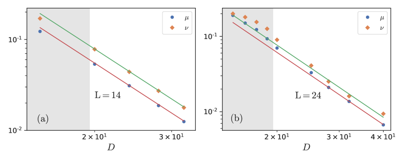
Figure 2: The data in Fig. 1 are fitted by $S=\mu\ln t$ and by $S_{N}=\frac{\nu}{2}\ln\ln t$. The plots show the prefactors $\mu,\nu$ extracted from these fits for a system size of (a) $L=14$ and (b) $L=24$ as a function of disorder strength $D$. The lines correspond to power-law fits $\sim 1/D^{\alpha}$ of $\mu,\nu$ deep in the MBL regime with $\alpha\approx 3$. The shaded area indicates the disorder regime where the system might be critical and the values of $\mu,\nu$ in this regime should be considered with care. For $L=14$ we simulated 10,000 disorder realizations starting from 50 random half-filled product states and in the case of $L=24$ we simulate 1500 disorder realization for $D\leq 28$ and 2000 for $D>28$ starting from a single random half-filled product state.

Most importantly, the time dependence of neither $S$ nor $S_{N}$ changes qualitatively. It is known that within the MBL phase but close to the transition rare regions with less disorder can cause a very slow dynamics [52, 53] and can destabilize the MBL phase in small systems. In order to exclude such a scenario, we also calculated the median of the entanglement and number entropies, shown in Fig. 3. The median quantities are defined by sorting the entropies for each realization in terms of magnitude at every point in time and then choosing the value in the middle, for an odd number of realizations, or the average of the two middle values, for an even number of realizations. The median number entropy shows the same double logarithmic growth in time as the average number entropy, shown in Fig. 1(b). We conclude that the observed long-time growth is not the consequence of rare regions but rather represents the typical behavior of the number entropy. The main qualitative difference between averaged and median entropies is a suppression of the initial increase in the median as compared to the average, i.e. rare regions do influence the short-time behavior but not the long-time scaling. More details about the dependence of $S_{N}$ on the disorder realizations are discussed in A.

The data thus do not support the notion that the growth of $S_{N}(t)$ changes in a qualitative manner if we move deeper into the putative MBL phase. The observed $S_{N}\sim\ln\ln t$ scaling rather seems to be an intrinsic property of the MBL phase—at least for the simulation times we are able to achieve numerically. Fig. 2 also indicates that the scaling of the total entanglement entropy $S$ and that of the number entropy $S_{N}$ are very closely linked. The prefactors of the logarithmic and double logarithmic fits show the same power-law dependence on disorder.

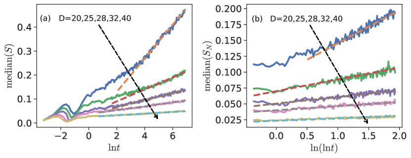
Figure 3: Numerical results for (a) the median of the von-Neumann entanglement entropy, and (b) the median of the number entropy for strong disorder, $D>D_{c}\sim 16$, for a system with $L=24$ sites. The dashed lines represent logarithmic fits in (a) and double logarithmic fits in (b). Here we calculate the median from 1500 disorder realization for $D\leq 28$ and from 2000 realizations for $D>28$ starting from a random half-filled product state.

3.2 Scaling with system size and disorder strength

Another question one might raise with regard to the interpretation of the results shown in Fig. 1 and Fig. 3, is whether the increase of $S_{N}$ is transient and will ultimately give way to saturation. A problem in addressing this issue is, of course, the limited system sizes which are amenable to a numerical solution. The best evidence that the behavior is not transient, is based on the following observation: For every system size $L$ and any $D>D_{c}$ there is a time $t_{d}$ where the numerical data start to deviate from $S_{N}=\frac{\nu}{2}\ln\ln t$ due to finite size effects. This is illustrated in Fig. 4(a,b) which also shows that this time $t_{d}$ is the same time where also the data for $S$ start to deviate from a logarithmic scaling, further supporting the notion that the growth of $S_{N}$ is linked to the growth of $S$. We have extracted the time $t_{d}$ from the numerical data and find that $t_{d}\sim\exp(L/\ell)$ where $\ell\sim(D-D_{c})^{-\alpha}$ is a characteristic length scale. This relation is illustrated in Fig. 4(c) where we observe an almost perfect scaling collapse of $t_{d}$ as function of $L/\ell$.

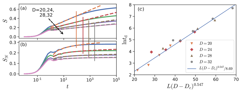
Figure 4: The time $t_{d}$ for $L=14$ where the numerical data for $S$ start to deviate from the fit $S=\mu\ln t$, shown in (a), is the same time where $S_{\mathrm{N}}$ starts to deviate from the fit $S_{N}=\frac{\nu}{2}\ln\ln t$, shown in (b). The data has been adopted from Fig. 2 in Ref. [26]. (c) $t_{d}$ depends on $L/\ell$ only with $\ell=(D-D_{c})^{-\alpha}$, $D_{c}\approx 16$, and $\alpha\approx 0.5$ leading to a scaling collapse. Over 10,000 disorder realizations starting from 50 random initial half-filled product states have been simulated. For the fitting process in (c), data for system sizes $L=10,12,14$ have been used.

We believe this to be a very strong indication that the observed growth of the number entropy is not transient. Based on this analysis, we expect that in the thermodynamic limit $S_{N}$ grows without bounds throughout the putative MBL phase.

3.3 $p(n)$ and truncated Hartley number entropy

Next, we want to address the possible criticism that the time regime in which we observe the double logarithmic scaling of the number entropy is a regime where $S_{N}<\ln 3$. The increase of the number entropy thus could potentially be explained by a single particle fluctuating between the two subsystems. In order to investigate this point, we have to consider the full particle number distribution $p(n)$. If indeed only small fluctuations around the initial particle number $n_{\text{ini}}$ in the subsystem contribute, then we expect that the distribution only changes in time for particle numbers close to this initial value, while $p(n)$ remains exponentially small for large fluctuations of $n$ away from this value at all times.

To investigate the change of the particle number distribution in time, we define for each sample its width by $\delta n_{c}=n_{\text{max}}-n_{\text{min}}$ with $p(n_{\text{max/min}})>p_{c}$. This is shown for one particular sample in Fig. 5(a).

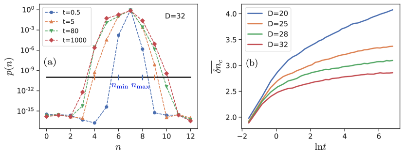
Figure 5: (a) Definition of the width $\delta n_{c}$ shown for a particle number distribution of a single disorder realization for $D=32,\,L=24$, and a cutoff $p_{c}=10^{-10}$. The ticks on the cutoff line show exemplarily $n_{\mathrm{min}}$ and $n_{\mathrm{max}}$ for $t=0.5$ and $t=5$. (b) Time evolution of the average width $\overline{\delta n_{c}}$ for a cutoff $p_{c}=10^{-10}$ for various disorder strengths. Here we simulated 1500 disorder realization for $D\leq 28$ and 2000 for $D>28$ starting from a random half-filled product state.

While the width $\delta n_{c}$ does depend on the value chosen for $p_{c}$, we find that the scaling of the average width is always given by $\overline{\delta n_{c}}\sim(\ln t)^{\nu}$ with some positive exponent $\nu$ provided that $p_{c}\ll 1$. This growth of the width of the particle number distribution is shown for different disorder strengths in Fig. 5(b). It is a clear indication that large particle number fluctuations do occur and that changes of $p(n)$ in time are not limited to redistributions close to $n=n_{\text{ini}}$ as would be expected if the MBL phase is truly localized.

Another way to see this, is to study the Hartley number entropy $S_{H}=\lim_{\alpha\to 0}S_{N}^{(\alpha)}$ [26]. The Hartley number entropy counts the particle numbers $n$ for which $p(n)\neq 0$. Since a unitary time evolution will immediately lead to a non-zero probability for any particle distribution consistent with the conservation laws, independent of whether or not the system is localized, it is important to introduce a cutoff $p_{c}>0$ and to only consider configurations with $p(n,t)>p_{c}$. All values below the cutoff are set to zero and the distribution is renormalized. If the system is in a localized phase, this truncated Hartley number entropy for any cutoff $p_{c}>0$ has to saturate in the thermodynamic limit at a value which is much below the equipartition value, corresponding to a fully thermalized infinite-temperature state. Only in the limit $p_{c}\to 0$ will $S_{H}$ asymptotically approach the equipartition value and a discrimination from an ergodic phase is no longer possible. Thus it is important to consider a truncated Hartley entropy with a non-zero cutoff $p_{c}$. We here choose a threshold $p_{c}$ which is well above the accuracy of our numerical calculations, which are done in double precision. Note that a relatively large cutoff will suppress the Hartley number entropy and make a distinction from the Anderson case impossible. Furthermore, we cannot take the limit $\alpha\to 0$ exactly numerically but rather consider a small but finite value of $\alpha=10^{-3}$. Results for the strongly disordered t-V model (1) with $V=2$ (MBL case) are compared to $V=0$ (Anderson case) in Fig. 6.

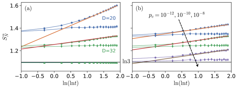
Figure 6: Truncated Hartley number entropies: (a) $S_{N}^{(\alpha)}$ with $\alpha=10^{-3}$ and $p_{c}=10^{-10}$ for the MBL case (circles) and the Anderson case (diamonds) for $L=24$. The lines are double logarithmic fits. Also shown are the entropies when only $p(\bar{n})$ and $p(\bar{n}\pm 1)$ are taken into account (triangles). The latter saturate at $\ln 3$. (b) Dependence of the results on the cutoff $p_{c}$ for a disorder strength $D=32$. Both figures are based on data already used in Fig. 5 and Fig. 6 in Ref. [26]. 1500 disorder realizations for $D\leq 28$ and 2000 for $D>28$ have been used starting from a single random half-filled product state.

There is a clear qualitative difference. While the Hartley number entropy quickly saturates in the Anderson case—showing that the possible particle numbers $n$ in the subsystem with $p(n)>p_{c}$ are limited, consistent with localization—$S_{H}$ continues to grow $\sim\ln\ln t$ similar to the number entropy shown in Fig. 1 and Fig. 3. In addition, we also show in Fig. 6 the entropies if only configurations with $p(\bar{n})$ and $p(\bar{n}\pm 1)$ are taken into account where $\bar{n}$ is the particle number with maximal probability. It is obvious, that these configurations alone cannot explain the observed growth of $S_{H}$. Finally, we note that while the cutoff $p_{c}$ does quantitatively change the results it does not change the $S_{H}\sim\ln\ln t$ growth.

In conclusion, the data presented in Fig. 5 and Fig. 6 clearly show that the observed increase of the particle number fluctuations after the quench cannot be explained by a small number of particles fluctuating between the subsystems. Instead, the probability for large particle number fluctuations is continuously growing in time in the putative MBL phase. This is inconsistent with a true localization of particles and is very different from the behavior observed in the Anderson localized phase. As a next step, we will try to shed some further light on the link between the von-Neumann entropy and the number entropy by deriving exact bounds for non-interacting fermionic and bosonic systems.

4 Bounds for number entropies and relation to particle fluctuations

From Fig. 1 , Fig. 3, and Fig. 4 we have seen that the $S\sim\ln t$ and $S_{N}\sim\ln\ln t$ growths of von-Neumann and number entropies seem to be linked. Due to the limiting procedure involved in obtaining $S$ and $S_{N}$, these quantities are difficult to work with in analytical calculations. Instead, we will concentrate on the second Rényi number entropy $S_{N}^{\left(2\right)}$ and the second Rényi entropy $S^{\left(2\right)}$ and start by considering Gaussian fermionic and bosonic systems. For these systems, we derive bounds for $S_{N}^{\left(2\right)}$ in terms of $S^{\left(2\right)}$. We will also clarify the connection between the number entropy and particle fluctuations $\Delta N=\sqrt{\langle N^{2}\rangle-\langle N\rangle^{2}}$. After deriving these exact relations for non-interacting systems, we will return to the interacting t-V model and show that similar relations also appear to hold in this case.

4.1 Exact bounds for free fermions and free bosons

In order to derive upper and lower bounds on the second Rényi number entropy $S_{N}^{\left(2\right)}$ in terms of particle fluctuations and the second Rényi entropy $S^{\left(2\right)}$, we make use of the fact that the quantum state for a non-interacting fermionic or bosonic system in any dimension is completely determined by its single-particle correlations and has a Gaussian form [54, 55]. Since we assume, furthermore, total particle number conservation, the density matrix $\rho$ can be represented as

$$\rho=\frac{1}{\mathcal{Z}}\mathtt{tr}\left[\exp\left(-{\displaystyle\sum\limits_{m,n}}c_{m}^{\dagger}C_{mn}c_{n}\right)\right],$$ (5)

where $c_{m}\left(c_{m}^{\dagger}\right)$ are the fermionic or bosonic annihilation (creation) operators at lattice site $m$. Here $\mathbf{C}$ is a Hermitian matrix which is determined entirely by single-particle correlations. The partition function $\mathcal{Z}=$ $\mathtt{tr}\Bigl{[}\exp\Bigl(-{\displaystyle\sum\limits_{m,n}}c_{m}^{\dagger}C_{mn}c_{n}\Bigr{missing})\Bigr{]}$ then reads

$$\mathcal{Z}=\det\left(1-se^{-\mathbf{C}}\right)^{-s},$$ (6)

where $s=1$ for bosons and $s=-1$ for fermions.

It is useful to introduce the moment generating function [56] of the total particle number $N=\sum\limits_{m}c_{m}^{\dagger}c_{m}$ in the considered partition in the form

$$\chi\left(\theta\right)=\mathtt{tr}\Bigl{(}\rho\exp\left(-i\theta N\right)\Bigr{)}={\displaystyle\sum\limits_{n=0}^{\infty}}p(n)\exp\left(-i\theta n\right),$$ (7)

whose Fourier coefficients are the probabilities $p(n)$ to find $n$ particles in the subsystem. It encodes all the information about the particle statistics. The moments of the distribution are given by the coefficients of the logarithm $\chi\left(\theta\right)$ [56, 39, 57]. In particular, the average particle number in the subsystem is given by

$$\langle N\rangle={\displaystyle\sum\limits_{n=0}^{\infty}}p(n)\,n=i\frac{\partial}{\partial\theta}\ln\chi\left(\theta\right)\bigr{|}_{\theta=0}\,$$ (8)

and the particle-number variance by

$$\Delta N^{2}={\displaystyle\sum\limits_{n=0}^{\infty}}p(n)\bigl{(}n-\langle N\rangle\bigr{)}^{2}=\left(i\frac{\partial}{\partial\theta}\right)^{2}\ln\chi\left(\theta\right)\bigr{|}_{\theta=0}\,.$$ (9)

4.1.1 Free fermions

For Gaussian fermionic states, the generating function can be written as a determinant

$$\chi\left(\theta\right)=\det\left[\mathbf{1}+\left(e^{-i\theta}-1\right)\frac{\mathbf{1}}{\mathbf{1}+e^{\mathbf{C}}}\right].$$ (10)

Making use of Parseval’s theorem one then finds

$$\sum_{n=0}^{\infty}p(n)^{2}=\frac{1}{2\pi}\int_{-\pi}^{\pi}d\theta\,\left|\chi\left(\theta\right)\right|^{2}=\frac{1}{2\pi}\int_{-\pi}^{\pi}d\theta\det\Bigl(\mathbf{1}-\mathbf{G}\left(1-\cos\theta\right)\Bigr{missing}),$$ (11)

where

$$\mathbf{G=}\frac{2e^{\mathbf{C}}}{\left(\mathbf{1}+e^{\mathbf{C}}\right)^{2}}$$ (12)

is a positive definite matrix and all eigenvalues are bounded by $1/2$. It is remarkable that, according to Eq.(9),  the number fluctuation $\Delta N^{2}$ are related to the eigenvalues of $\mathbf{G}$ in the following simple way

$$\Delta N^{2}=\frac{\mathtt{tr}\,\mathbf{G}}{2}.$$ (13)

In order to derive bounds for $S_{N}^{\left(2\right)}$ in terms of $S^{\left(2\right)}$ we also need a relationship between the correlation matrix $\mathbf{G}$ and the second Rényi entropy $S^{\left(2\right)}$

$$S^{\left(2\right)}=-\ln\mathtt{tr}\rho^{2}=-\mathtt{tr}\ln\left(1-\mathbf{G}\right).$$ (14)

Now we are ready to derive the promised bounds for $S_{N}^{\left(2\right)}$ in terms of the number fluctuations and the second Rényi entropy.

Upper bound

By using the identity $\det A=\exp(\mathtt{tr}\ln A)$ for any positive definite matrix $A$, expression (11) can be written as

$$\sum_{n=0}^{\infty}p(n)^{2} = \frac{2}{\pi}\int_{0}^{\pi/2}\!\!\!d\theta\,\exp\left[\mathtt{tr}\,\ln\left(\mathbf{1}-2\mathbf{G}\sin^{2}\theta\right)\right]$$ (15)

$$\geq \frac{2}{\pi}\int_{0}^{\pi/2}\!\!\!d\theta\,\exp\left[2\mathtt{tr}\,\mathbf{G}\ln\left(1-\sin^{2}\theta\right)\right]=\frac{\Gamma\left(\frac{1}{2}+4\Delta N^{2}\right)}{\sqrt{\pi}\Gamma\left(1+4\Delta N^{2}\right)},$$ (16)

where in the last line we have used the fact that $2\mathbf{G}\leq 1$ and the inequality

$$x\frac{\ln(1-b)}{b}\geq\ln\left(1-x\right)\geq x\frac{\ln\left(1-a\right)}{a},$$ (17)

which holds for $0\leq b\leq x\leq a\leq 1$. These inequalities follow simply from the fact that the function $\frac{\ln(1-x)}{x}$ is a monotonously decreasing function of $x$. Then the integral can be calculated elementary in terms of the gamma function, i.e. $\frac{2}{\pi}\int_{0}^{\pi/2}d\theta\,\cos^{p}\theta=\frac{\Gamma\left(\frac{1+p}{2}\right)}{\sqrt{\pi}\Gamma\left(1+\frac{p}{2}\right)},$ for $p>-1$. The inequality (16) yields the following bound

$$S_{N}^{\left(2\right)}=-\ln\left(\sum_{n}p(n)^{2}\right)\leq\ln\frac{\sqrt{\pi}\Gamma\left(1+4\Delta N^{2}\right)}{\Gamma\left(\frac{1}{2}+4\Delta N^{2}\right)}.$$ (18)

It is easy to see, using the asymptotic expansions of Bessel and Gamma functions, that for large $\Delta N$ the right hand side of this inequality coincides with the lower bound for $S_{N}^{\left(2\right)}$ given in [24, 25]:

$$S_{N}^{\left(2\right)}\geq 2\Delta N^{2}-\ln\left[I_{0}\left(2\Delta N^{2}\right)\right]\,\xrightarrow[\Delta N>1]{\,}\ln\left(2\sqrt{\pi}\Delta N\right).$$ (19)

Hence, $S_{N\text{ }}^{\left(2\right)}$ can actually be approximated as

$$S_{N\text{ }}^{\left(2\right)}\approx\ln\left(2\sqrt{\pi}\Delta N\right)$$ (20)

for large values of $\Delta N$.

We note that the bound (18) is much better than the modified version of Shannon’s inequality [58] for discrete variables

$$S_{N}^{\left(2\right)}\leq\ln\sqrt{2\pi e\left(\Delta N^{2}+\frac{1}{12}\right)},$$ (21)

which becomes $S_{N}^{\left(2\right)}=0\leq\ln\sqrt{\frac{2\pi e}{12}}$ at $\Delta N\rightarrow 0$ (i.e., it reduces to a trivial one). Despite being a sharp bound on $S_{N}^{\left(2\right)}$ for large $\Delta N,$ a comparison with the lower bound (19) shows (18) is not tight for small $\Delta N$. We therefore now derive another upper bound on $S_{N}^{\left(2\right)}$ for small $\Delta N^{2}\leq\frac{1}{2}$.

Since $S_{N}^{\left(2\right)}$ does not account for the different configurations of particles, an obvious upper bound on $S_{N}^{\left(2\right)}$ is given by the total Rényi entropy

$$S_{N}^{\left(2\right)}\leq S^{\left(2\right)}=-\mathtt{tr}\ln\left(1-\mathbf{G}\right)\leq-\ln\left(1-\mathtt{tr}\mathbf{G}\right)=-\ln\left(1-2\Delta N^{2}\right)$$ (22)

which holds for $\Delta N^{2}\leq\frac{1}{2}.$

By combining this inequality with (18) we arrive at

$$S_{N}^{\left(2\right)}\leq\left\{\begin{array}[]{c}-\ln\left(1-2\Delta N^{2}\right)\text{ \ \ if }\Delta N\leq\frac{1}{2}\\ \ln\frac{\sqrt{\pi}\Gamma\left(1+4\Delta N^{2}\right)}{\Gamma\left(\frac{1}{2}+4\Delta N^{2}\right)}\text{ \ if }\Delta N>\frac{1}{2}\end{array}\right..$$ (23)

We note that this bound is tight for small as well as for large $\Delta N$.

Lower bound

As shown in Ref. [24], the inequality (19)—providing a lower bound for $S_{N}^{(2)}$—is valid for any non-interacting fermion system in any dimension. We now show that this lower bound can be further improved. To this end we show that

$$S_{N}^{(2)}=-\ln\sum_{n}p(n)^{2}\geq\Phi\left(2\Delta N^{2},S^{\left(2\right)}\right),$$ (24)

where

$$\Phi\left(2\Delta N^{2},S^{\left(2\right)}\right)=-\ln\left\{\frac{e^{-2\Delta N^{2}}}{2}\bigl{[}I_{0}\left(2\Delta N^{2}\right)+L_{0}\left(2\Delta N^{2}\right)\bigr{]}+\frac{e^{-S^{\left(2\right)}}}{2}\left[I_{0}\left(S^{\left(2\right)}\right)-L_{0}\left(S^{\left(2\right)}\right)\right]\right\}.$$ (25)

Here $L_{0}\left(x\right)$ is the modified Struve function. Since $S^{\left(2\right)}\geq 2\Delta N^{2}$ (which follows from the obvious inequality $\ln(1-x)\leq-x$, for $0\leq x\leq 1$ ), and $\frac{\exp\left(-x\right)}{2}\left[I_{0}\left(x\right)-L_{0}\left(x\right)\right]$ being a monotonously decreasing function, we see that this bound is better than our previous bound derived in [24] which was based on the inequality

$$\sum_{n}p(n)^{2}\leq\exp\left(-2\Delta N^{2}\right)I_{0}\left(2\Delta N^{2}\right).$$ (26)

In order to proof inequality (24), we split the integral

$$\sum_{n=0}^{\infty}p(n)^{2}=\frac{2}{\pi}\int_{0}^{\pi/2}\!\!\!d\theta\,\exp\left[\mathtt{tr}\ln\left(\mathbf{1}-2\mathbf{G}\sin^{2}\theta\right)\right]=U_{1}+U_{2}$$

into two parts $U_{1}$ and $U_{2}$, where

$$U_{1} = \frac{2}{\pi}\int_{0}^{\frac{\pi}{4}}\!\!\!d\theta\,\exp\left[\mathtt{tr}\ln\left(\mathbf{1}-2\mathbf{G}\sin^{2}\theta\right)\right],$$ (27)

$$U_{2} = \frac{2}{\pi}\int_{0}^{\frac{\pi}{4}}\!\!\!d\theta\,\exp\left[\mathtt{tr}\ln\left(\mathbf{1}-2\mathbf{G}\cos^{2}\theta\right)\right].$$ (28)

The first integral can be bounded from above by using the arithmetic-geometric inequality and the integral can then be calculated elementary in terms of the modified Bessel and Struve functions of the first kind resulting in

$$U_{1}\leq\frac{\exp\left(-2\Delta N^{2}\right)}{2}\left[I_{0}\left(2\Delta N^{2}\right)+L_{0}\left(2\Delta N^{2}\right)\right].$$ (29)

Using (17) and the fact that $\cos^{2}\theta\geq\frac{1}{2}$ for $0\leq\theta\leq$ $\frac{\pi}{4},$ we find for the second integral

$$U_{2} \leq \frac{2}{\pi}\int_{0}^{\frac{\pi}{4}}\!\!\!d\theta\,\exp\left[2\cos^{2}\theta\,\mathtt{tr}\,\ln\left(\mathbf{1}-\mathbf{G}\right)\right]=\frac{2}{\pi}\int_{0}^{\frac{\pi}{4}}\!\!\!d\theta\,\exp\left[-2S^{\left(2\right)}\cos^{2}\theta\right]$$ (30)

$$= \frac{1}{2}\exp\left(-S^{\left(2\right)}\right)\left[I_{0}\left(S^{\left(2\right)}\right)-L_{0}\left(S^{\left(2\right)}\right)\right].$$

Combining Eq. (30) with Eq.(29) one obtains expressions (24) and (25). The derived lower bound depends on $\Delta N$ and $S^{\left(2\right)}$. Making use, furthermore, of either $\Delta N^{2}\geq S^{(2)}/(4\ln(2))$ [59, 60, 24] for large $\Delta N$ or $2\Delta N^{2}\geq 1-e^{-S(2)}$ (see Eq. (22)) for small $\Delta N$, we arrive at the following connection between the entropies

$$S_{N}^{\left(2\right)}\geq\left\{\begin{array}[]{c}\Phi\left(1-e^{-S^{\left(2\right)}},S^{\left(2\right)}\right)\text{ \ if \ }S^{\left(2\right)}\leq\ln 2,\\ \Phi\left(\frac{S^{\left(2\right)}}{2\ln 2},S^{\left(2\right)}\right)\text{ \ if \ }S^{\left(2\right)}>\ln 2\end{array}\right..$$ (31)

We now present numerical checks for the quality of the derived bounds and estimates for fermionic Gaussian models with and without disorder. In Fig. 7(a), the time evolution of $S^{(2)}_{N}$ for the Hamiltonian (1) with $V=D=0$ is shown.

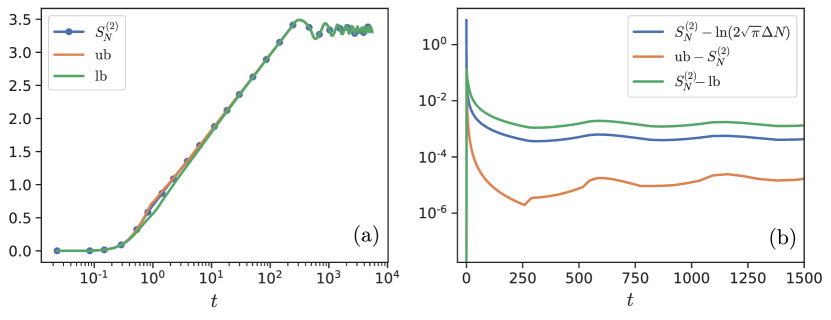
Figure 7: (a) $S^{(2)}_{N}$ for the model (1) with $V=D=0$ and $L=1024$ starting from a charge-density wave inital state compared to the upper bound (ub) (23) and the lower bound (lb) (24). The bounds are quite tight as shown by the differences between $S^{(2)}_{N}$ and the two bounds in panel (b). Also $S^{(2)}_{N}$ can be well approximated by $\ln(2\sqrt{\pi}\Delta N)$.

The upper and lower bounds are very tight in this case. In Fig. 7(b) it is shown that the second number Rényi entropy is closely related to the particle number fluctuations. At long times, the difference between the two decays exponentially before reaching a lower limit due to the saturation of both quantities in a finite system.

Next, we consider free fermionic systems with potential disorder (Anderson case) and off-diagonal disorder. For the Anderson case, shown in Fig. 8(a,b), tight bounds can be obtained both for weak and strong disorder.

Figure 8: $S^{(2)}_{N}$ for the Anderson localized case, Eq. (1) with $V=0$, for (a) $L=512$ and weak disorder, and (b) $L=128$ and strong disorder. Averages over 2000 disorder realizations starting from a random half-filled product state are shown. (c) Free fermions with the random hopping amplitude $J_{j}$ drawn from a box distribution, the so-called off-diagonal disorder (ODD) case, for $L=1024$ and averaged over 20,000 disorder realizations starting from a random half-filled product state. Shown are the upper bound (ub) corresponding to Eq. (23) and the lower bound (lb) given by Eq. (24). For previous results where other bounds were used to constrain $S^{(2)}$ by $S_{N}$, see Ref. [24].

In addition, we also present in Fig. 8(c) results for the Hamiltonian (1) with $V=D=0$ and with the hopping amplitude $J$ replaced by a position dependent hopping amplitude $J_{j}$ which is drawn from a box distribution. In this so-called off-diagonal disorder (ODD) case, the entanglement entropy increases as $S^{(2)}\sim\ln\ln t$ while the number entropy scales as $S_{N}^{(2)}\sim\ln\ln\ln t$ [61, 24].

4.1.2 Free Bosons

In this section we derive, for completeness, upper and lower bounds on the second Rényi number entropy for a Gaussian bosonic state.

Upper bound

The generating function $\chi\left(\theta\right)$ in the bosonic case can be written as

$$\chi\left(\theta\right)=\det\left[\mathbf{1}-\left(e^{-i\theta}-1\right)\frac{\mathbf{1}}{e^{\mathbf{C}}-\mathbf{1}}\right]^{-1}.$$ (32)

For bosons the matrix $\mathbf{C}$ is positive definite. Making use of Parseval’s theorem, one then finds for the number purity

$$\sum_{n=0}^{\infty}p(n)^{2}=\frac{1}{2\pi}\int_{-\pi}^{\pi}\!\!\!d\theta\,\frac{1}{\det\left(\mathbf{1}+\mathbf{W}\left(1-\cos\theta\right)\right)},\qquad\mbox{where}\quad\mathbf{W}=\frac{2e^{\mathbf{C}}}{\left(e^{\mathbf{C}}-1\right)^{2}}.$$ (33)

The steps for obtaining bounds for $S_{N}^{\left(2\right)}$ are the same as in the case of free fermions. We apply the arithmetic-geometric inequality to get an upper bound on $\det\left(\mathbf{1}+\mathbf{W}\left(1-\cos\theta\right)\right)$, which then yields

$$\sum_{n=0}^{\infty}p(n)^{2}\geq\exp\left(-\mathtt{tr}\mathbf{W}\right)I_{0}\left(\mathtt{tr}\mathbf{W}\right).$$ (34)

Furthermore, using Eq. (9), one can show that $\mathtt{tr}\mathbf{W}$ gives the fluctuations of the total particle number, i.e. $\mathtt{tr}\mathbf{W}=2\Delta N^{2}$. With inequality (34) we arrive at the following upper bound

$$S_{N}^{\left(2\right)}=-\ln\left(\sum_{n=0}^{\infty}p(n)^{2}\right)\leq-\ln\left[\exp\left(-2\Delta N^{2}\right)I_{0}\left(2\Delta N^{2}\right)\right].$$ (35)

We see that this upper bound on $S_{N}^{\left(2\right)}$ for bosons coincides with the fermionic lower bound (19) in terms of the particle number fluctuations.

Lower Bound

By making use of the inequality $\ln\left(1+x\right)\geq\frac{\ln\left(1+a\right)}{a}x,$   $0\leq x\leq a$, we have

$$\sum_{n=0}^{\infty}p(n)^{2} = \frac{1}{\pi}\int_{0}^{\pi}\!\!\!d\theta\,\exp\left(-\mathtt{tr\ln}\left[1+2\mathbf{W}\sin^{2}\frac{\theta}{2}\right]\right)$$

$$\leq \int_{0}^{\pi}\!\!\!d\theta\,\exp\left(-\sin^{2}\frac{\theta}{2}\mathtt{tr\ln}\left[1+2\mathbf{W}\right]\right)=\exp\left(-S^{\left(2\right)}\right)I_{0}\left(S^{\left(2\right)}\right),$$

where in the last line we have used the identity $S^{\left(2\right)}=\frac{1}{2}\mathtt{tr}\ln\left(\mathbf{1}+2\mathbf{W}\right)$. Hence, we arrive at the lower bound

$$S_{N}^{\left(2\right)}\geq-\ln\left[\exp\left(-S^{\left(2\right)}\right)I_{0}\left(S^{\left(2\right)}\right)\right]\,.$$ (37)

4.2 Relation between number entropy and number fluctuations for interacting systems

In the previous section, we have established a tight relation between the Rényi number entropy $S_{N}^{(2)}$ and the number fluctuations $\Delta N$ in non-interacting, i.e. Gaussian systems, expressed by the lower and upper bounds, Eqs. (19) and (23), respectively,

$$2\Delta N^{2}-\ln\left[I_{0}\left(2\Delta N^{2}\right)\right]\leq S_{N}^{\left(2\right)}\leq\left\{\begin{array}[]{c}-\ln\left(1-2\Delta N^{2}\right)\text{ \ \ if }\Delta N\leq\frac{1}{2}\\ \ln\frac{\sqrt{\pi}\Gamma\left(1+4\Delta N^{2}\right)}{\Gamma\left(\frac{1}{2}+4\Delta N^{2}\right)}\text{ \ if }\Delta N>\frac{1}{2}\end{array}\right..$$ (38)

A natural question that arises is whether these bounds also hold for interacting systems. In Fig. 9, we show the number entropy as well as the lower bound (lb), and the upper bound (ub) for the $t-V$ model without disorder. We recognize that the two bounds as well as the estimate, $S_{N}^{(2)}\approx\ln\bigl(2\sqrt{\pi}\Delta N\bigr{missing})$ for large $\Delta N$, hold true even in the interacting case. Since both quantities $S^{(2)}_{N}$ and $\Delta N$ depend on the same probability distribution $p(n)$, this might not be too surprising. It does show, however, that an unlimited growth of the Rényi number entropy implies a corresponding growth of number fluctuations. Numerical results for $\Delta N$ in the putative MBL phase are discussed in B.

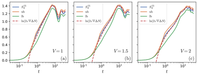
Figure 9: Results for the dynamics of the number entropy $S_{N}^{(2)}$ for $L=24$ when quenching the $t-V$ model from a charge-density wave initial state compared to the upper bound (ub) (23) and the lower bound (lb) (19) for different interaction strengths but without disorder. Furthermore, we can see that $S_{N}^{(2)}\approx\mathrm{ln}(2\sqrt{\pi}\Delta N)$ holds even in the interacting case.

4.3 Renormalized bounds for the number entropy in terms of the entanglement entropy for interacting systems

The bounds for the number entropy derived above for Gaussian, i.e. non-interacting, systems also establish a relation to the entanglement entropy

$$S^{(2)}_{N}\sim\ln S^{(2)}.$$ (39)

This relation is consistent with our observation that $S^{(2)}\sim\ln t$ and $S^{(2)}_{N}\sim\ln\ln t$ in the putative many-body localized phase. In the following, we show that the lower bound for $S_{N}^{(2)}$ in terms of $S^{(2)}$, which leads to relation (39), indeed appears to hold also for the interacting t-V model including in the MBL phase with some renormalization. This provides further evidence that the particle fluctuations are not bounded.

To this end, we introduce a renormalization prefactor $\gamma\leq 1$ in (31), see also [25]

$$S_{N}^{(2)}\geq\left\{\begin{array}[]{c}\gamma\Phi\left(1-e^{-S^{\left(2\right)}},S^{\left(2\right)}\right)\text{ \ if \ }S^{\left(2\right)}\leq\ln 2,\\ \gamma\Phi\left(\frac{S^{\left(2\right)}}{2\ln 2},S^{\left(2\right)}\right)\text{ \ if \ }S^{\left(2\right)}>\ln 2\end{array}\right..$$ (40)

The factor $\gamma$ is needed as the lower bound will be broken at some point in time otherwise. We compare $S_{N}^{(2)}$ to the renormalized lower bound, see Fig. 10, for the disordered $t-V$ model. We find that this bound describes the data very well both for $D<D_{c}$ and for $D>D_{c}$. As can be seen in Fig. 10(c), the prefactor $\gamma$ does depend smoothly on the disorder strength. We find, in particular, that $\gamma$ is almost constant for $D<D_{c}$ and falls off approximately like a power law above $D_{c}$.

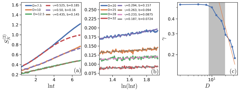
Figure 10: Dynamics of $S_{N}^{(2)}$ for $L=24$ compared to the renormalized lower bound (40) (dashed lines) for (a) $D<D_{c}$, and (b) $D>D_{c}$. The renormalized lower bounds are shifted by a constant $b$ to demonstrate that the bound shows the same scaling as $S^{(2)}_{N}$. (a-b) are partially based on data already used in Ref. [25]. (c) Renormalization factor $\gamma$ as a function of disorder. For $D<D_{c}$, $\gamma$ remains close to $\gamma\sim 0.5$ but decays approximately like a power-law for $D>D_{c}$. Here we have averaged over 1500 disorder realizations for $D\leq 28$ and 2000 for $D\geq 28$, starting from a random half-filled product state.

5 Conclusions

In conclusion, we have provided strong arguments why the putative MBL phase in the disordered one-dimensional t-V model (isotropic Heisenberg chain) does not appear to be truly localized. Our arguments are based on the numerical evaluation of the time evolution after a quantum quench, the results of which are summarized in Table 1. In the interacting case, our simulations have been carried out in systems up to lengths of $L=24$. We therefore obviously cannot exclude scenarios where the behavior of the particle fluctuations qualitatively changes for larger system sizes and longer times than numerically accessible. We note, however, that if one is going to dismiss the results presented here as valid arguments against localization, one should then also dismiss any arguments in favor of localization coming from numerical studies of small systems. This would ultimately mean that we currently cannot numerically study whether or not MBL phases exist.

Phase	disorder	interaction	$S^{(2)}$	$S_{N}^{(2)}$
AL	potential, $D\neq 0$	non-interacting	$\sim\mbox{const}$	$\sim\mbox{const}$
ODD	off-diagonal	non-interacting	$\sim\ln\ln t$	$\sim\ln\ln\ln t$
MBL	potential, $D>D_{c}$	interacting	$\sim\ln t$	$\sim\ln\ln t$
clean	no-disorder	non-int. & int.	$\sim t$	$\sim\ln t$

Table 1: Asymptotic growth of Rényi entropy $S^{(2)}$ and Rényi number entropy $S_{N}^{(2)}$ following a quantum quench for various phases of the t-V model. The relation $S_{N}^{(2)}\sim\ln S^{(2)}$ appears to hold in all of them.

If we assume that we can learn something about putative MBL phases in one dimension from studies of small systems, then it appears to be clear that the evidence now points towards an absence of true localization. Our original arguments made in Ref. [25] were based on the observation that the number entropy grows as $S_{N}\sim\ln\ln t$ and that this growth is consistent with the relation $S_{N}\sim\ln S$ thus pointing to an unbounded growth of the number entropy.

In the present article, we have tried to address possible criticisms of this interpretation of the data. First of all, we have shown that all the data for disorder strengths close to the assumed ergodic-MBL phase transition at $D=D_{c}$ up to disorder strengths of more than $2D_{c}$ are consistently described by $S_{N}=\frac{\nu}{2}\ln\ln t$ and that the prefactor $\nu$ shows a power-law dependence on disorder strength. Furthermore, calculating the median of the number entropy we showed that the observed scaling represents typical behavior and is not the result of rare disorder realizations. This indicates that the increase of the number entropy is a generic feature of the MBL phase and not restricted to disorder strengths close to the phase transition. Second, we have demonstrated that the deviation time $t_{d}$, where the finite-size data start to deviate from the double logarithmic fit, scales as $t_{d}\sim\exp(L/\ell)$ with a characteristic length scale $\ell\sim(D-D_{c})^{-0.5}$, which is well defined only for $D>D_{c}$. We have shown that all the data for $t_{d}$, obtained for various different system sizes and disorder strengths, show an excellent scaling collapse. The double logarithmic scaling of the number entropy in time therefore does not appear to be transient but rather indicative of the thermodynamic limit. Lastly, we have shown that the observed increase of the number entropy cannot be explained by the fluctuations of a small number of particles initially situated near the cut between the two subsystems. Instead, we have found that the particle number distribution $p(n)$ as a whole becomes wider over time. In particular, large particle number fluctuations are becoming increasingly more likely. This is most clearly seen in the truncated Hartley number entropy $S_{H}$ which counts the number of particle configurations $n$ with $p(n)>p_{c}$ where $p_{c}$ is some cutoff. We have shown that $S_{H}\sim\ln\ln t$ for the putative MBL phase while $S_{H}$ saturates quickly in the Anderson case.

To shed some more light on the relation between the growth of the entanglement and number entropies, we have considered free fermionic and bosonic systems. In both cases, we have been able to derive strict upper and lower bounds and have numerically shown that these bounds can be very tight in specific cases. We have argued that these bounds, with renormalized coefficients, also hold in the putative MBL phase further supporting the conclusion that $S_{N}\sim\ln S$, i.e., the unbounded logarithmic growth of the entanglement entropy is accompanied by an unbounded double logarithmic growth of the number entropy. In light of these findings, we believe that the very notion of many-body localization in one dimension needs to be reconsidered.

Finally, we would like to emphasize again that we have not made any statements about the putative ergodic-MBL phase transition so far. We can think of at least two scenarios for the phase diagram of the t-V model which are consistent with our data: (1) One possibility would be that there is no phase transition but rather a crossover with the particle dynamics becoming slower and slower with increasing disorder. Such a scenario would appear to be consistent with recent results in Refs. [20, 21, 22, 23]. We want to point out, in particular, that $S\sim\ln(t)\sim(t^{\nu}-1)/\nu$ and $S_{N}\sim\ln\ln(t)\sim\ln[(t^{\nu}-1)/\nu]$ for $\nu$ small, i.e., a crossover where $\nu\to 0$ for $D\to\infty$ would be very difficult to distinguish numerically from a true change in scaling at a phase transition. We note that in this case sub-diffusive transport would prevail at very long times $t^{\nu}\gg 1$ for a small but finite $\nu$. (2) A second possibility might be that there is indeed a phase transition at a critical disorder strength $D_{c}$ with the system for $D>D_{c}$ having both extended and localized states. In this regard, we note that the observed scaling of the entanglement entropy and the number entropy appears to be the same as the one recently found right at the phase transition in the three-dimensional Anderson model [62]. I.e., the phase for $D>D_{c}$ could be more akin to an extended critical phase. If such a transition would be at all possible and what the nature of such a transition would be is, however, unclear.

It would also be of interest to conduct similar studies of the Rényi number entropies and particle fluctuations in interacting disordered many-body systems in higher dimensions. We note that in this case the instability of MBL in the thermodynamic limit appears to be far less controversial although the situation is far from completely settled either [63, 64, 65, 66].

Appendix A Number entropy for different realizations

An important question for the interpretation of our results is whether or not the observed scaling of the number entropy $S_{N}\sim\ln\ln t$ is related to rare configurations and rare initial states. In Sec. 3.1, we have tried to answer this question by comparing the average with the median entropy and found the same scaling for both quantities. Here we want to go one step further and consider the number entropy for samples sorted into ten bins according to the magnitude of $S_{N}(t)$ at each time step and averaged over each bin individually. The result for two disorder strengths is shown in Fig. 1.

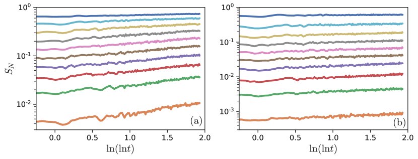
Figure 1: Number entropies for (a) $D=20$ and (b) $D=32$. Here we have sorted all samples into ten bins at each time step and averaged over each bin individually.

We find that almost all the bins show a scaling $S_{N}\sim\ln\ln t$. For the bin containing the samples with the largest values of $S_{N}$, the number entropy rises quickly to values close to their finite-size saturation values, i.e., for the rare samples which do contain regions with little disorder the saturation value is reached even quicker in time. This further supports the notion that the double logarithmic scaling in time is the typical behavior for all $D>D_{c}$ and is not related to any special rare configurations.

Appendix B Number fluctuations

We have found it useful to concentrate mostly on the Rényi number entropies instead of studying the particle number fluctuations $\Delta N$ in a partition directly. The main reason to do so is that the scaling of the number entropy can be directly related to the $S\sim\ln t$ scaling of the entanglement entropy which is supposed to be one of the hallmarks of the putative MBL phase. In particular, we have shown that it is possible to derive bounds for $S_{N}^{(2)}$ in terms of $S^{(2)}$ for Gaussian systems which also appear to hold for the interacting case. Nevertheless, the Rényi number entropies $S^{(\alpha)}_{N}$ and the particle fluctuations $\Delta N$ in a subsystem depend of course both on the same particle distribution function $p(n)$. We therefore expect that $\Delta N(t)$ is also continuously growing in time. That this is indeed the case is shown in Fig. 1.

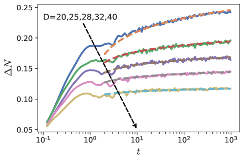
Figure 1: Averaged particle number fluctuations $\Delta N$ in one partition as a function of time. The lines are fits $\Delta N\sim(\ln t)^{\nu}+b$.

We find that the data for all disorder strengths are well fitted by $\Delta N\sim(\ln t)^{\nu}+b$ which is consistent with the results for the Rényi number entropies presented in the main text.

References

- [1] P. W. Anderson, Absence of diffusion in certain random lattices, Phys. Rev. 109 (1958) 1492–1505.
- [2] E. Abrahams (Ed.), 50 Years of Anderson Localization, World Scientific, Singapore, 2010.
- [3] E. Abrahams, P. W. Anderson, D. C. Licciardello, T. V. Ramakrishnan, Scaling theory of localization: Absence of quantum diffusion in two dimensions, Phys. Rev. Lett. 42 (1979) 673–676. doi:10.1103/PhysRevLett.42.673.
- [4] J. T. Edwards, D. J. Thouless, Numerical studies of localization in disordered systems, J. Phys. C 5 (8) (1972) 807.
- [5] V. Oganesyan, D. A. Huse, Localization of interacting fermions at high temperature, Phys. Rev. B 75 (2007) 155111.
- [6] A. Pal, D. A. Huse, Many-body localization phase transition, Phys. Rev. B 82 (2010) 174411.
- [7] T. Enss, F. Andraschko, J. Sirker, Many-body localization in infinite chains, Phys. Rev. B 95 (2017) 045121.
- [8] D. M. Basko, I. L. Aleiner, B. L. Altshuler, Metal-insulator transition in a weakly interacting many-electron system with localized single-particle states, Ann. Phys.
- [9] J. Z. Imbrie, Diagonalization and many-body localization for a disordered quantum spin chain, Phys. Rev. Lett. 117 (2016) 027201.
- [10] D. J. Luitz, N. Laflorencie, F. Alet, Many-body localization edge in the random-field heisenberg chain, Phys. Rev. B 91 (2015) 081103.
- [11] M. Žnidarič, T. Prosen, P. Prelovšek, Many-body localization in the heisenberg magnet in a random field, Phys. Rev. B 77 (2008) 064426.
- [12] J. H. Bardarson, F. Pollmann, J. E. Moore, Unbounded growth of entanglement in models of many-body localization, Phys. Rev. Lett. 109 (2012) 017202. doi:10.1103/PhysRevLett.109.017202.
- [13] M. Serbyn, Z. Papić, D. A. Abanin, Local conservation laws and the structure of the many-body localized states, Phys. Rev. Lett. 111 (2013) 127201.
- [14] D. A. Huse, R. Nandkishore, V. Oganesyan, Phenomenology of fully many-body-localized systems, Phys. Rev. B 90 (2014) 174202.
- [15] R. Vosk, D. A. Huse, E. Altman, Theory of the many-body localization transition in one-dimensional systems, Phys. Rev. X 5 (2015) 031032.
-
[16]
A. Goremykina, R. Vasseur, M. Serbyn,
Analytically
solvable renormalization group for the many-body localization transition,
Phys. Rev. Lett. 122 (2019) 040601.
doi:10.1103/PhysRevLett.122.040601.
URL https://link.aps.org/doi/10.1103/PhysRevLett.122.040601 -
[17]
P. T. Dumitrescu, A. Goremykina, S. A. Parameswaran, M. Serbyn, R. Vasseur,
Kosterlitz-thouless
scaling at many-body localization phase transitions, Phys. Rev. B 99 (2019)
094205.
doi:10.1103/PhysRevB.99.094205.
URL https://link.aps.org/doi/10.1103/PhysRevB.99.094205 - [18] A. C. Potter, R. Vasseur, S. A. Parameswaran, Universal properties of many-body delocalization transitions, Phys. Rev. X 5 (2015) 031033.
- [19] A. Morningstar, D. A. Huse, J. Z. Imbrie, Many-body localization near the critical point, Phys. Rev. B 102 (2020) 125134.
- [20] J. Suntajs, J. Bonca, T. Prosen, L. Vidmar, Quantum chaos challenges many-body localization, arXiv: 1905.06345.
- [21] J. Suntajs, J. Bonca, T. Prosen, L. Vidmar, Ergodicity breaking transition in finite disordered spin chains, arXiv: 2004.01719.
- [22] D. Sels, A. Polkovnikov, Dynamical obstruction to localization in a disordered spin chain, arXiv: 2009.04501.
- [23] T. LeBlond, D. Sels, A. Polkovnikov, M. Rigol, Universality in the onset of quantum chaos in many-body systems, arXiv: 2012.07849.
- [24] M. Kiefer-Emmanouilidis, R. Unanyan, J. Sirker, M. Fleischhauer, Bounds on the entanglement entropy by the number entropy in non-interacting fermionic systems, SciPost Phys. 8 (2020) 083.
- [25] M. Kiefer-Emmanouilidis, R. Unanyan, M. Fleischhauer, J. Sirker, Evidence for unbounded growth of the number entropy in many-body localized phases, Phys. Rev. Lett. 124 (2020) 243601.
- [26] M. Kiefer-Emmanouilidis, R. Unanyan, M. Fleischhauer, J. Sirker, Absence of true localization in many-body localized phases, arXiv:2010.00565.
- [27] F. Andraschko, T. Enss, J. Sirker, Purification and many-body localization in cold atomic gases, Phys. Rev. Lett. 113 (2014) 217201.
-
[28]
E. V. H. Doggen, F. Schindler, K. S. Tikhonov, A. D. Mirlin, T. Neupert, D. G.
Polyakov, I. V. Gornyi,
Many-body
localization and delocalization in large quantum chains, Phys. Rev. B 98
(2018) 174202.
doi:10.1103/PhysRevB.98.174202.
URL https://link.aps.org/doi/10.1103/PhysRevB.98.174202 -
[29]
E. V. H. Doggen, A. D. Mirlin,
Many-body
delocalization dynamics in long aubry-andré quasiperiodic chains, Phys.
Rev. B 100 (2019) 104203.
doi:10.1103/PhysRevB.100.104203.
URL https://link.aps.org/doi/10.1103/PhysRevB.100.104203 - [30] D. A. Abanin, J. H. Bardarson, G. de Tomasi, S. Gopalakrishnan, V. Khemani, S. A. Parameswaran, F. Pollmann, A. C. Potter, M. Serbyn, R. Vasseur, Distinguishing localization from chaos: challenges in finite-size systems, arXiv: 1911.04501.
-
[31]
P. Sierant, D. Delande, J. Zakrzewski,
Thouless time
analysis of anderson and many-body localization transitions, Phys. Rev.
Lett. 124 (2020) 186601.
doi:10.1103/PhysRevLett.124.186601.
URL https://link.aps.org/doi/10.1103/PhysRevLett.124.186601 -
[32]
W. Buijsman, V. Cheianov, V. Gritsev,
Sensitivity of
the spectral form factor to short-range level statistics, Phys. Rev. E 102
(2020) 042216.
doi:10.1103/PhysRevE.102.042216.
URL https://link.aps.org/doi/10.1103/PhysRevE.102.042216 -
[33]
D. J. Luitz, Y. B. Lev,
Absence of slow
particle transport in the many-body localized phase, Phys. Rev. B 102 (2020)
100202.
doi:10.1103/PhysRevB.102.100202.
URL https://link.aps.org/doi/10.1103/PhysRevB.102.100202 - [34] I. Klich, L. S. Levitov, Scaling of entanglement entropy and superselection rules, arXiv:0812.0006.
-
[35]
H. M. Wiseman, J. A. Vaccaro,
Entanglement of
indistinguishable particles shared between two parties, Phys. Rev. Lett. 91
(2003) 097902.
doi:10.1103/PhysRevLett.91.097902.
URL https://link.aps.org/doi/10.1103/PhysRevLett.91.097902 -
[36]
M. R. Dowling, A. C. Doherty, H. M. Wiseman,
Entanglement of
indistinguishable particles in condensed-matter physics, Phys. Rev. A 73
(2006) 052323.
doi:10.1103/PhysRevA.73.052323.
URL https://link.aps.org/doi/10.1103/PhysRevA.73.052323 -
[37]
N. Schuch, F. Verstraete, J. I. Cirac,
Nonlocal
resources in the presence of superselection rules, Phys. Rev. Lett. 92
(2004) 087904.
doi:10.1103/PhysRevLett.92.087904.
URL https://link.aps.org/doi/10.1103/PhysRevLett.92.087904 -
[38]
N. Schuch, F. Verstraete, J. I. Cirac,
Quantum
entanglement theory in the presence of superselection rules, Phys. Rev. A 70
(2004) 042310.
doi:10.1103/PhysRevA.70.042310.
URL https://link.aps.org/doi/10.1103/PhysRevA.70.042310 -
[39]
H. F. Song, C. Flindt, S. Rachel, I. Klich, K. Le Hur,
Entanglement
entropy from charge statistics: Exact relations for noninteracting many-body
systems, Phys. Rev. B 83 (2011) 161408.
doi:10.1103/PhysRevB.83.161408.
URL https://link.aps.org/doi/10.1103/PhysRevB.83.161408 -
[40]
T. Rakovszky, C. W. von Keyserlingk, F. Pollmann,
Entanglement
growth after inhomogenous quenches, Phys. Rev. B 100 (2019) 125139.
doi:10.1103/PhysRevB.100.125139.
URL https://link.aps.org/doi/10.1103/PhysRevB.100.125139 - [41] G. Parez, R. Bonsignori, P. Calabrese, Quasiparticle dynamics of symmetry resolved entanglement after a quench: the examples of conformal field theories and free fermionsarXiv:2010.09794.
-
[42]
H. F. Song, S. Rachel, C. Flindt, I. Klich, N. Laflorencie, K. Le Hur,
Bipartite
fluctuations as a probe of many-body entanglement, Phys. Rev. B 85 (2012)
035409.
doi:10.1103/PhysRevB.85.035409.
URL https://link.aps.org/doi/10.1103/PhysRevB.85.035409 -
[43]
R. Bonsignori, P. Ruggiero, P. Calabrese,
Symmetry resolved
entanglement in free fermionic systems, Journal of Physics A: Mathematical
and Theoretical 52 (47) (2019) 475302.
doi:10.1088/1751-8121/ab4b77.
URL https://doi.org/10.1088%2F1751-8121%2Fab4b77 -
[44]
S. Murciano, G. D. Giulio, P. Calabrese,
Symmetry resolved
entanglement in gapped integrable systems: a corner transfer matrix
approach, SciPost Phys. 8 (2020) 46.
doi:10.21468/SciPostPhys.8.3.046.
URL https://scipost.org/10.21468/SciPostPhys.8.3.046 - [45] S. Murciano, G. D. Giulio, P. Calabrese, Entanglement and symmetry resolution in two dimensional free quantum field theories, JHEP 2020 (2020) 73.
- [46] A. Lukin, M. Rispoli, R. Schittko, M. E. Tai, A. M. Kaufman, S. Choi, V. Khemani, J. Leonard, M. Greiner, Probing entanglement in a many-body-localized system, Science 364 (2019) 256.
- [47] T. Bridges, A. Elben, P. Jurcevic, B. Vermersch, C. Maier, B. P. Lanyon, P. Zoller, R. Blatt, C. F. Roos, Probing rényi entanglement entropy via randomized measurements, Science 364 (2019) 260. doi:10.1126/science.aau4963.
- [48] H. F. Trotter, On the product of semi-groups of operators, Proc. Amer. Math. Soc. 10 (1959) 545.
- [49] M. Suzuki, Generalized trotter’s formula and systematic approximants of exponential operators and inner derivations with applications to many-body problems, Commun. Math. Phys. 51 (1976) 183.
- [50] M. Suzuki, Transfer-matrix method and monte carlo simulation in quantum spin systems, Phys. Rev. B 31 (1985) 2957.
- [51] D. J. Luitz, N. Laflorencie, F. Alet, Extended slow dynamical regime close to the many-body localization transition, Phys. Rev. B 93 (2016) 060201.
-
[52]
S. Gopalakrishnan, M. Müller, V. Khemani, M. Knap, E. Demler, D. A. Huse,
Low-frequency
conductivity in many-body localized systems, Phys. Rev. B 92 (2015) 104202.
doi:10.1103/PhysRevB.92.104202.
URL https://link.aps.org/doi/10.1103/PhysRevB.92.104202 -
[53]
K. Agarwal, E. Altman, E. Demler, S. Gopalakrishnan, D. A. Huse, M. Knap,
Rare-region
effects and dynamics near the many-body localization transition, Annalen der
Physik 529 (7) (2017) 1600326.
arXiv:https://onlinelibrary.wiley.com/doi/pdf/10.1002/andp.201600326,
doi:https://doi.org/10.1002/andp.201600326.
URL https://onlinelibrary.wiley.com/doi/abs/10.1002/andp.201600326 - [54] I. Peschel, On the reduced density matrix for a chain of free electrons, J. Stat. Mech. (2004) P06004.
- [55] I. Peschel, V. Eisler, Reduced density matrices and entanglement entropy in free lattice models, J. Phys. A 42 (50) (2009) 504003.
-
[56]
I. Klich, L. Levitov,
Quantum noise
as an entanglement meter, Phys. Rev. Lett. 102 (2009) 100502.
doi:10.1103/PhysRevLett.102.100502.
URL https://link.aps.org/doi/10.1103/PhysRevLett.102.100502 -
[57]
P. Calabrese, M. Mintchev, E. Vicari,
Exact relations
between particle fluctuations and entanglement in fermi gases, EPL
(Europhysics Letters) 98 (2) (2012) 20003.
doi:10.1209/0295-5075/98/20003.
URL https://doi.org/10.1209%2F0295-5075%2F98%2F20003 - [58] T. M. Cover, J. A. Thomas, Elements of information theory, Wiley, New York, (1991).
-
[59]
I. Klich, Lower
entropy bounds and particle number fluctuations in a fermi sea, Journal of
Physics A: Mathematical and General 39 (4) (2006) L85–L91.
doi:10.1088/0305-4470/39/4/l02.
URL https://doi.org/10.1088%2F0305-4470%2F39%2F4%2Fl02 -
[60]
D. Muth, R. G. Unanyan, M. Fleischhauer,
Dynamical
simulation of integrable and nonintegrable models in the heisenberg picture,
Phys. Rev. Lett. 106 (2011) 077202.
doi:10.1103/PhysRevLett.106.077202.
URL https://link.aps.org/doi/10.1103/PhysRevLett.106.077202 - [61] Y. Zhao, F. Andraschko, J. Sirker, Entanglement entropy of disordered quantum chains following a global quench, Phys. Rev. B 93 (2016) 205146.
-
[62]
Y. Zhao, D. Feng, Y. Hu, S. Guo, J. Sirker,
Entanglement
dynamics in the three-dimensional anderson model, Phys. Rev. B 102 (2020)
195132.
doi:10.1103/PhysRevB.102.195132.
URL https://link.aps.org/doi/10.1103/PhysRevB.102.195132 -
[63]
J.-y. Choi, S. Hild, J. Zeiher, P. Schauß, A. Rubio-Abadal, T. Yefsah,
V. Khemani, D. A. Huse, I. Bloch, C. Gross,
Exploring the
many-body localization transition in two dimensions, Science 352 (6293)
(2016) 1547–1552.
arXiv:https://science.sciencemag.org/content/352/6293/1547.full.pdf,
doi:10.1126/science.aaf8834.
URL https://science.sciencemag.org/content/352/6293/1547 - [64] T. B. Wahl, A. Pal, S. H. Simon, Signatures of the many-body localized regime in two dimensions, Nat. Phys. 15 (2019) 164.
-
[65]
S. c. v. Grozdanov, A. Lucas, S. Sachdev, K. Schalm,
Absence of
disorder-driven metal-insulator transitions in simple holographic models,
Phys. Rev. Lett. 115 (2015) 221601.
doi:10.1103/PhysRevLett.115.221601.
URL https://link.aps.org/doi/10.1103/PhysRevLett.115.221601 -
[66]
S. c. v. Grozdanov, A. Lucas, K. Schalm,
Incoherent thermal
transport from dirty black holes, Phys. Rev. D 93 (2016) 061901.
doi:10.1103/PhysRevD.93.061901.
URL https://link.aps.org/doi/10.1103/PhysRevD.93.061901