Fast and Furious: Real Time End-to-End 3D Detection, Tracking and Motion Forecasting with a Single Convolutional Net

Abstract

In this paper we propose a novel deep neural network that is able to jointly reason about 3D detection, tracking and motion forecasting given data captured by a 3D sensor. By jointly reasoning about these tasks, our holistic approach is more robust to occlusion as well as sparse data at range. Our approach performs 3D convolutions across space and time over a bird’s eye view representation of the 3D world, which is very efficient in terms of both memory and computation. Our experiments on a new very large scale dataset captured in several north american cities, show that we can outperform the state-of-the-art by a large margin. Importantly, by sharing computation we can perform all tasks in as little as 30 ms.

1 Introduction

Modern approaches to self-driving divide the problem into four steps: detection, object tracking, motion forecasting and motion planning. A cascade approach is typically used where the output of the detector is used as input to the tracker, and its output is fed to a motion forecasting algorithm that estimates where traffic participants are going to move in the next few seconds. This is in turn fed to the motion planner that estimates the final trajectory of the ego-car. These modules are usually learned independently, and uncertainty is usually rarely propagated. This can result in catastrophic failures as downstream processes cannot recover from errors that appear at the beginning of the pipeline.

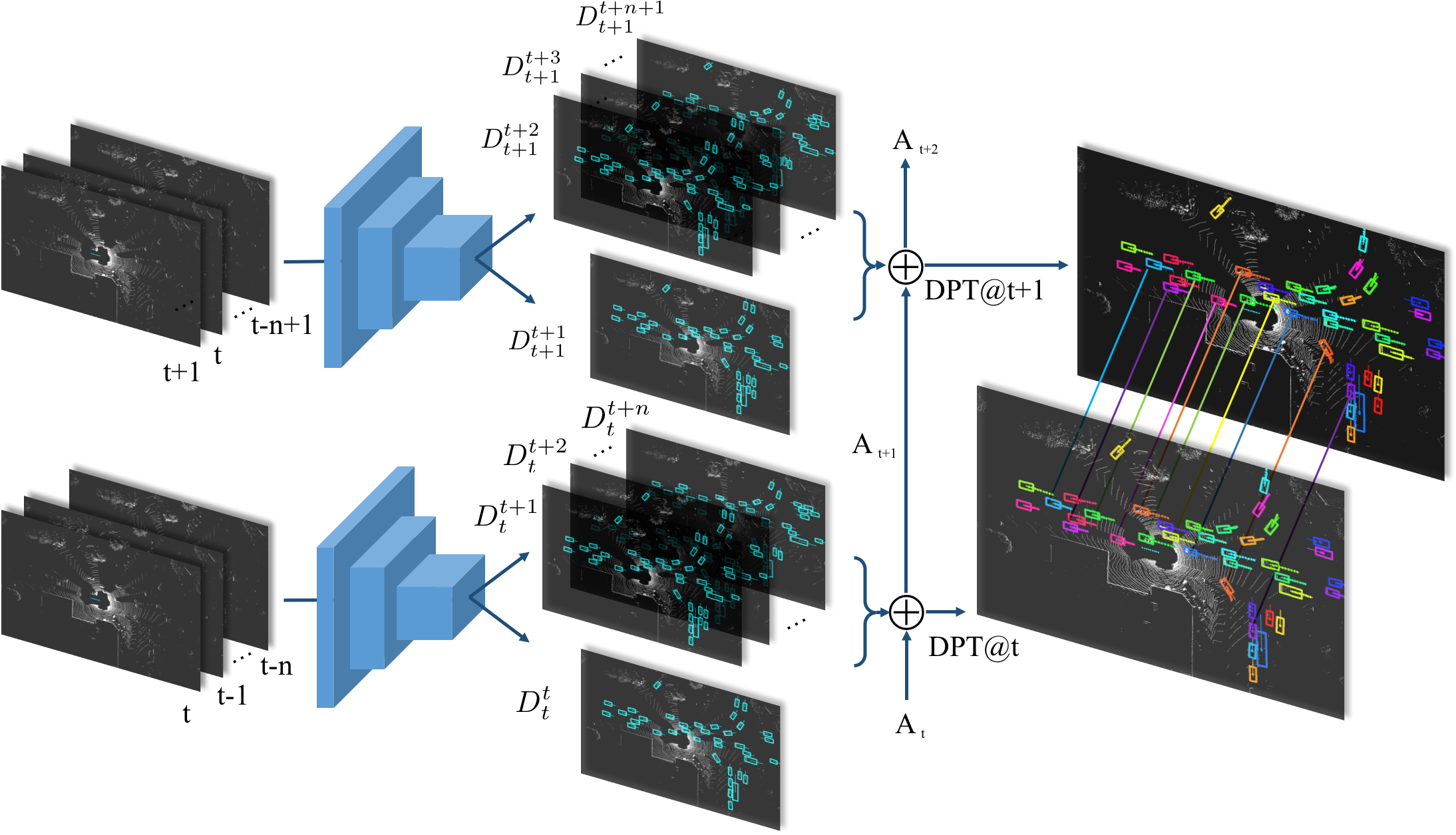
Figure 1: Overview of our approach: Our $FaF$ network takes multiple frames as input and performs detection, tracking and motion forecasting.

In contrast, in this paper we propose an end-to-end fully convolutional approach that performs simultaneous 3D detection, tracking and motion forecasting by exploiting spatio-temporal information captured by a 3D sensor. We argue that this is important as tracking and prediction can help object detection. For example, leveraging tracking and prediction information can reduce detection false negatives when dealing with occluded or far away objects. False positives can also be reduced by accumulating evidence over time. Furthermore, our approach is very efficient as it shares computations between all these tasks. This is extremely important for autonomous driving where latency can be fatal.

We take advantage of 3D sensors and design a network that operates on a bird-eye-view (BEV) of the 3D world. This representation respects the 3D nature of the sensor data, making the learning process easier as the network can exploit priors about the typical sizes of objects.

Our approach is a one-stage detector that takes a 4D tensor created from multiple consecutive temporal frames as input and performs 3D convolutions over space and time to extract accurate 3D bounding boxes. Our model produces bounding boxes not only at the current frame but also multiple timestamps into the future. We decode the tracklets from these predictions by a simple pooling operation that combine the evidence from past and current predictions.

We demonstrate the effectiveness of our model on a very large scale dataset captured from multiple vehicles driving in North-america and show that our approach significantly outperforms the state-of-the-art. Furthermore, all tasks take as little as 30ms.

2 Related Work

2D Object Detection:

Over the last few years many methods that exploit convolutional neural networks to produce accurate 2D object detections, typically from a single image, have been developed. These approaches typically fell into two categories depending on whether they exploit a first step dedicated to create object proposals. Modern two-stage detectors [24, 8, 4, 11], utilize region proposal networks (RPN) to learn the region of interest (RoI) where potential objects are located. In a second stage the final bounding box locations are predicted from features that are average-pooled over the proposal RoI. Mask-RCNN [8] also took this approach, but used RoI aligned features addressing theboundary and quantization effect of RoI pooling. Furthermore, they added an additional segmentation branch to take advantage of dense pixel-wise supervision, achieving state-of-the-art results on both 2D image detection and instance segmentation. On the other hand one-stage detectors skip the proposal generation step, and instead learn a network that directly produces object bounding boxes. Notable examples are YOLO [23], SSD [17] and RetinaNet [16]. One-stage detectors are computationally very appealing and are typically real-time, especially with the help of recently proposed architectures, e.g. MobineNet [10], SqueezeNet [31]. One-stage detectors were outperformed significantly by two stage-approaches until Lin et al. [16] shown state-of-the-art results by exploiting a focal loss and dense predictions.

3D Object Detection:

In robotics applications such as autonomous driving we are interested in detecting objects in 3D space. The ideas behind modern 2D image detectors can be transferred to 3D object detection. Chen et al. [2] used stereo images to perform 3D detection. Li [15] used 3D point cloud data and proposed to use 3D convolutions on a voxelized representation of point clouds. Chen et al. [3] combined image and 3D point clouds with a fusion network. They exploited 2D convolutions in BEV, however, they used hand-crafted height features as input. They achieved promising results on KITTI [6] but only ran at 360ms per frame due to heavy feature computation on both 3D point clouds and images. This is very slow, particularly if we are interested in extending these techniques to handle temporal data.

Object Tracking:

Over the past few decades many approaches have been develop for object tracking. In this section we briefly review the use of deep learning in tracking. Pretrained CNNs were used to extract features and perform tracking with correlation [18] or regression [29, 9]. Wang and Yeung [30] used an autoencoder to learn a good feature representation that helps tracking. Tao et al. [27] used siamese matching networks to perform tracking. Nam and Han [21] finetuned a CNN at inference time to track object within the same video.

Motion Forecasting:

This is the problem of predicting where each object will be in the future given multiple past frames. Lee et al. [14] proposed to use recurrent networks for long term prediction. Alahi et al. [1] used LSTMs to model the interaction between pedestrian and perform prediction accordingly. Ma et al. [19] proposed to utilize concepts from game theory to model the interaction between pedestrian while predicting future trajectories. Some work has also focussed on short term prediction of dynamic objects [7, 22]. [28] performed prediction for dense pixel-wise short-term trajectories using variational autoencoders. [26, 20] focused on predicting the next future frames given a video, without explicitly reasoning about per pixel motion.

Multi-task Approaches:

Feichtenhofer et al. [5] proposed to do detection and tracking jointly from video. They model the displacement of corresponding objects between two input images during training and decode them into object tubes during inference time.

Different from all the above work, in this paper we propose a single network that takes advantage of temporal information and tackles the problem of 3D detection, short term motion forecasting and tracking in the scenario of autonomous driving. While temporal information provides us with important cues for motion forecasting, holistic reasoning allows us to better propagate the uncertainty throughout the network, improving our estimates. Importantly, our model is super efficient and runs real-time at 33 FPS.

3 Joint 3D Detection, Tracking and Motion Forecasting

In this work, we focus on detecting objects by exploiting a sensor which produces 3D point clouds. Towards this goal, we develop a one-stage detector which takes as input multiple frames and produces detections, tracking and short term motion forecasting of the objects’ trajectories into the future. Our input representation is a 4D tensor encoding an occupancy grid of the 3D space over several time frames. We exploit 3D convolutions over space and time to produce fast and accurate predictions. As point cloud data is inherently sparse in 3D space, our approach saves lots of computation as compared to doing 4D convolutions over 3D space and time. We name our approach Fast and Furious (FaF), as it is able to create very accurate estimates in as little as 30 ms.

In the following, we first describe our data parameterization in Sec. 3.1 including voxelization and how we incorporate temporal information. In Sec. 3.2, we present our model’s architecture, follow by the objective we use for training the network (Sec. 3.3).

3.1 Data Parameterization

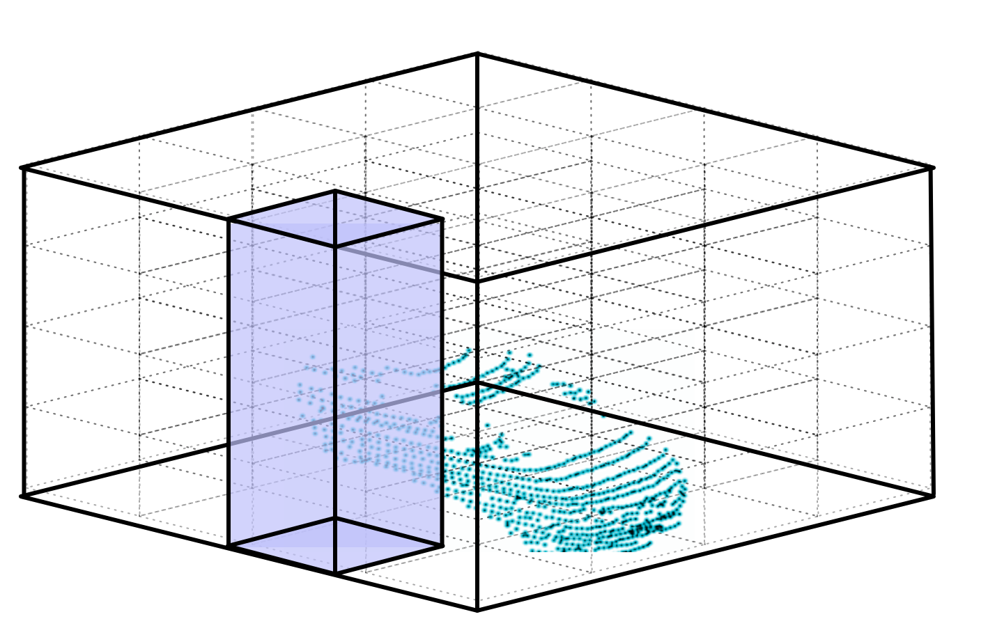
Figure 2: Voxel Representation: using height directly as input feature.

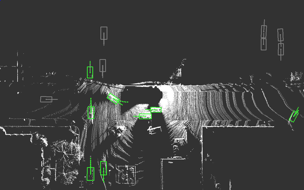
Figure 3: Overlay temporal & motion forecasting data. Green: bbox w/ 3D point. Grey: bbox w/o 3D point

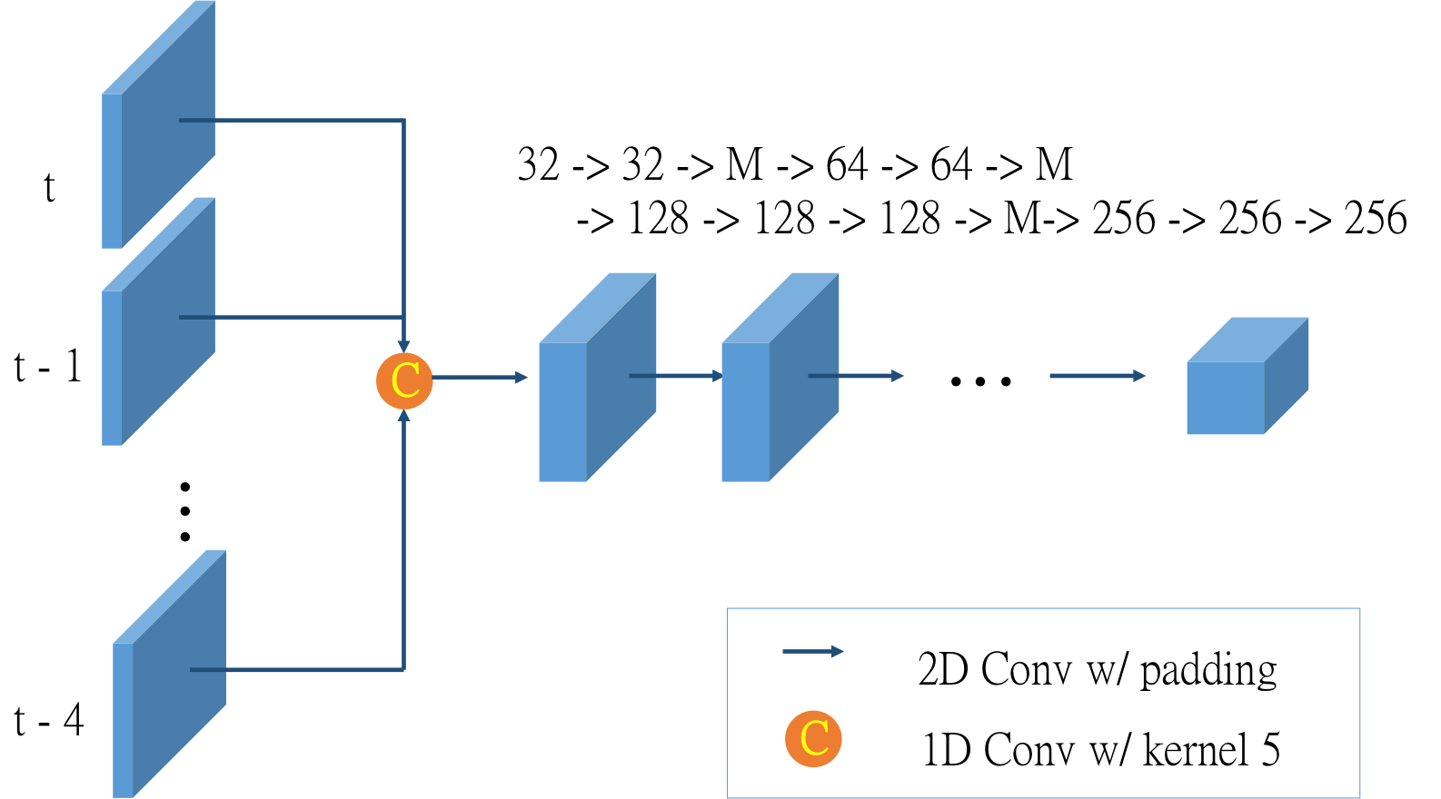
(a) Early fusion

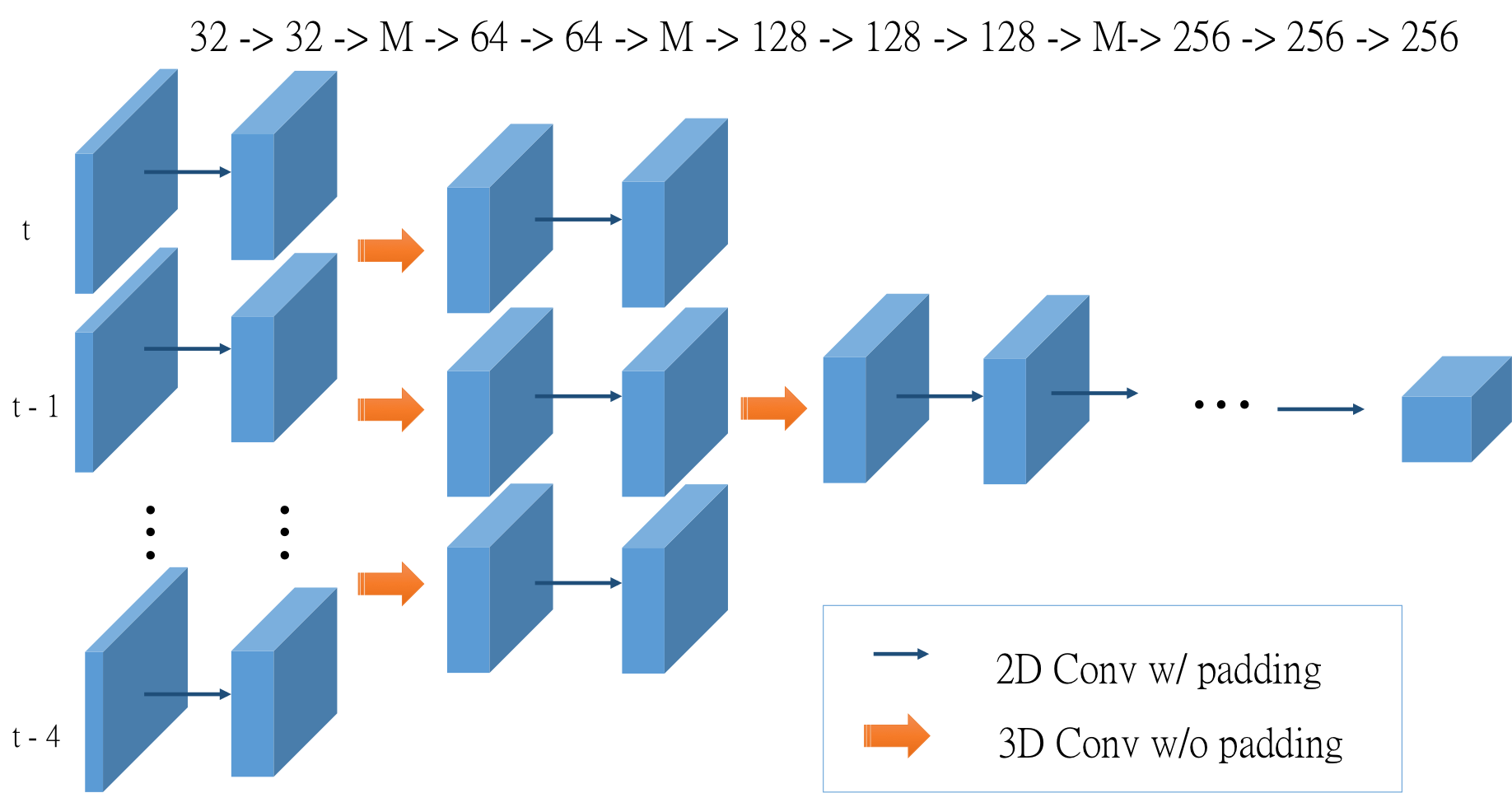
(b) Later fusion

Figure 4: Modeling temporal information

In this section, we first describe our single frame representation of the world. We then extend our representation to exploit multiple frames.

Voxel Representation:

In contrast to image detection where the input is a dense RGB image, point cloud data is inherently sparse and provides geometric information about the 3D scene. In order to get a representation where convolutions can be easily applied, we quantize the 3D world to form a 3D voxel grid. We then assign a binary indicator for each voxel encoding whether the voxel is occupied. We say a voxel is occupied if there exists at least one point in the voxel’s 3D space. As the grid is a regular lattice, convolutions can be directly used. We do not utilize 3D convolutions on our single frame representation as this operation will waste most computation since the grid is very sparse, i.e., most of the voxels are not occupied. Instead, we performed 2D convolutions and treat the height dimension as the channel dimension. This allows the network to learn to extract information in the height dimension. This contrast approaches such as MV3D [3], which perform quantization on the x-y plane and generate a representation of the z-dimension by computing hand-crafted height statistics. Note that if our grid’s resolution is high, our approach is equivalent to applying convolution on every single point without loosing any information. We refer the reader to Fig. 2 for an illustration of how we construct the 3D tensor from 3D point cloud data.

Adding Temporal Information:

In order to perform motion forecasting, it is crucial to consider temporal information. Towards this goal, we take all the 3D points from the past $n$ frames and perform a change of coordinates to represent then in the current vehicle coordinate system. This is important in order to undo the ego-motion of the vehicle where the sensor is mounted.

After performing this transformation, we compute the voxel representation for each frame. Now that each frame is represented as a 3D tensor, we can append multiple frames’ along a new temporal dimension to create a 4D tensor. This not only provides more 3D points as a whole, but also gives cues about vehicle’s heading and velocity enabling us to do motion forecasting. As shown in Fig. 3, where for visualization purposes we overlay multiple frames, static objects are well aligned while dynamic objects have ‘shadows’ which represents their motion.

3.2 Model Formulation

Our single-stage detector takes a 4D input tensor and regresses directly to object bounding boxes at different timestamps without using region proposals. We investigate two different ways to exploit the temporal dimension on our 4D tensor: early fusion and late fusion. They represent a tradeoff between accuracy and efficiency, and they differ on at which level the temporal dimension is aggregated.

Early Fusion:

Our first approach aggregates temporal information at the very first layer. As a consequence it runs as fast as using the single frame detector. However, it might lack the ability to capture complex temporal features as this is equivalent to producing a single point cloud from all frames, but weighting the contribution of the different timestamps differently. In particular, as shown in Fig. 4, given a 4D input tensor, we first use a 1D convolution with kernel size $n$ on temporal dimension to reduce the temporal dimension from $n$ to 1. We share the weights among all feature maps, i.e., also known as group convolution. We then perform convolution and max-pooling following VGG16 [25] with each layer number of feature maps reduced by half. Note that we remove the last convolution group in VGG16, resulting in only 10 convolution layers.

Late Fusion:

In this case, we gradually merge the temporal information. This allows the model to capture high level motion features. We use the same number of convolution layers and feature maps as in the early fusion model, but instead perform 3D convolution with kernel size $3\times 3\times 3$ for 2 layers without padding on temporal dimension, which reduces the temporal dimension from $n$ to 1, and then perform 2D spatial convolution with kernel size $3\times 3$ for other layers. We refer the reader to Fig. 4 for an illustration of our architecture.

We then add two branches of convolution layers as shown in Fig. 5. The first one performs binary classification to predict the probability of being a vehicle. The second one predicts the bounding box over the current frame as well as $n-1$ frames into the future. Motion forecasting is possible as our approach exploits multiple frames as input, and thus can learn to estimate useful features such as velocity and acceleration.

Following SSD [17], we use multiple predefined boxes for each feature map location. As we utilize a BEV representation which is metric, our network can exploit priors about physical sizes of objects. Here we use boxes corresponding to 5 meters in the real world with aspect ratio of $1:1,1:2,2:1,1:6,6:1$ and 8 meters with aspect ratio of $1:1$. In total there are 6 predefined boxes per feature map location denoted as $a_{i,j}^{k}$ where $i=1,...,I,j=1,...,J$ is the location in the feature map and $k=1,...,K$ ranges over the predefined boxes (i.e., size and aspect ratio). Using multiple predefined boxes allows us to reduce the variance of regression target, thus makes the network easy to train. Notice that we do not use predefined heading angles. Furthermore we use both $\sin$ and $\cos$ values to avoid the $180$ degrees ambiguity.

In particular, for each predefined box $a_{i,j}^{k}$, our network predicts the corresponding normalized location offset $\hat{l_{x}},\hat{l_{y}}$, log-normalized sizes $\hat{s_{w}},\hat{s_{h}}$ and heading parameters $\hat{a}_{\sin},\hat{a}_{\cos}$.

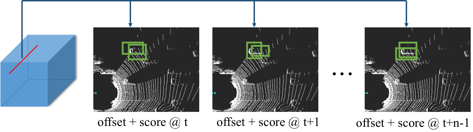
Figure 5: Motion forecasting

Decoding Tracklets:

At each timestamp, our model outputs the detection bounding boxes for $n$ timestamps. Reversely, each timestamp will have current detections as well as $n-1$ past predictions. Thus we can aggregate the information for the past to produce accurate tracklets without solving any trajectory based optimization problem. Note that if detection and motion forecasting are perfect, we can decode perfect tracklets. In practice, we use average as aggregation function. When there is overlap between detections from current and past’s future predictions, they are considered to be the same object and their bounding boxes will simply be averaged. Intuitively, the aggregation process helps particularly when we have strong past predictions but no current evidence, e.g., if the object is currently occluded or a false negative from detection. This allow us to track through occlusions over multiple frames. On the other hand, when we have strong current evidence but not prediction from the past, then there is evidence for a new object.

3.3 Loss Function and Training

We train the network to minimize a combination of classification and regression loss. In the case of regression we include both the current frame as well as our $n$ frames forecasting into the future. That is

$$\ell(w)=\sum\left(\alpha\cdot\ell_{\text{cla}}(w)+\sum\limits_{i=t,t+1,...,t+n}\ell_{\text{reg}}^{t}(w)\right)$$ (1)

where $t$ is the current frame and $w$ represents the model parameters.

We employ as classification loss binary cross-entropy computed over all locations and predefined boxes:

$$\ell_{\text{cla}}(w)=\sum_{i,j,k}q_{i,j,k}\log p_{i,j,k}(w)$$ (2)

Here $i,j,k$ are the indices on feature map locations and predefined box identity, $q_{i,j,k}$ is the class label (i.e. $q_{i,j,k}$ =1 for vehicle and 0 for background) and $p_{i,j,k}$ is the predicted probability for vehicle.

In order to define the regression loss for our detections and future predictions, we first need to find their associated ground truth. We defined their correspondence by matching each predefined box against all ground truth boxes. In particular, for each predicted box, we first find the ground truth box with biggest overlap in terms of intersection over union (IoU). If the IoU is bigger than a fixed threshold ($0.4$ in practice), we assign this ground truth box as $\bar{a}_{i,j}^{k}$ and assign 1 to its corresponding label $q_{i,j,k}$. Following SSD [17], if there exist a ground truth box not assigned to any predefined box, we will assign it to its highest overlapping predefined box ignoring the fixed threshold. Note that multiple predefined boxes can be associated to the same ground truth, and some predefined boxes might not have any correspondent ground truth box, meaning their $q_{i,j,k}=0$.

Thus we define the regression targets as

$$l_{x} =\frac{x-x^{GT}}{w^{GT}} l_{y} =\frac{y-y^{GT}}{h^{GT}}$$

$$s_{w} =\log\frac{w}{w^{GT}} s_{h} =\log\frac{h}{h^{GT}}$$

$$a_{sin} =\sin(\theta^{GT}) a_{cos} =\cos(\theta^{GT})$$

We use a weighted smooth L1 loss over all regression targets where smooth L1 is defined as:

$$\textrm{smooth}_{L_{1}}(\hat{x},x)=\begin{cases}\frac{1}{2}(\hat{x}-x)^{2}&\text{if }|\hat{x}-x|<1\\ |\hat{x}-x|-\frac{1}{2}&\text{otherwise}\end{cases}$$ (3)

Hard Data Mining

Due to the imbalance of positive and negative samples, we use hard negative mining during training. We define positive samples as those predefined boxes having corresponding ground truth box, i.e., $q_{i,j,k}=1$. For negative samples, we rank all candidates by their predicted score $p_{i,j,k}$ from the classification branch and take the top negative samples with a ration of 3 in practice.

IoU	0.5	0.6	0.7	0.8	0.9	Time [ms]
SqueezeNet_v1.1 [12]	85.80	81.06	69.97	43.20	3.70	9
SSD [17]	90.23	86.76	77.92	52.39	5.87	23
MobileNet [10]	90.56	87.05	78.39	52.10	5.64	65
FaF	93.24	90.54	83.10	61.61	11.83	30

Table 1: Detection performance on $144\times 80$ meters region, with object having $\geq$ 3 number 3D points

4 Experimental Evaluation

Unfortunately there is no publicly available dataset which evaluates 3D detection, tracking and motion forecasting. We thus collected a very large scale dataset in order to benchmark our approach. It is 2 orders of magnitude bigger than datasets such as KITTI [6].

Dataset:

Our dataset is collected by a roof-mounted LiDAR on top of a vehicle driving around several North-American cities. It consists of 546,658 frames collected from 2762 different scenes. Each scene consists of a continuous sequence. Our validation set consists of 5,000 samples collected from 100 scenes, i.e., 50 continuous frames are taken from each sequence. There is no overlap between the geographic area where the training and validation are collected, in order to showcase strong generalization. Our labels might contain vehicles with no 3D point on them as the labelers have access to the full sequence in order to provide accurate annotations. Our labels contain 3D rotated bounding box as well as track id for each vehicle.

Training Setup:

At training time, we use a spatial X-Y region of size $144\times 80$ meters, where each grid cell is $0.2\times 0.2$ meters. On the height dimension, we take the range from -2 to 3.5 meters with a 0.2 meter interval, leading to 29 bins. For temporal information, we take all the 3D points from the past 5 timestamps. Thus our input is a 4 dimensional tensor consisting of time, height, X and Y.

For both our early-fusion and late-fusion models, we train from scratch using Adam optimizer [13] with a learning rate of 1e-4. The model is trained on a 4 Titan XP GPU server with batch size of 12. We train the model for 100K iteration with learning rate halved at 60K and 80K iterations respectively.

Detection Results:

We compare our model against state-of-the-art real-time detectors including SSD [17], MobileNet [10] and SqueezeNet [12]. Note that these detectors are all developed to work on 2D detection from images. To make them competitive, we also build our predefined boxes into their system, which further easy the task for those detectors. The region of interest is $144\times 80M$ centered at ego-car during inference time. We keeps the same voxelization for all models and evaluate detections against ground truth vehicle bounding boxes with at minimum of three 3D points. Vehicles with less than three points are considered don’t care regions. We consider a detection correct if it has an IoU against any ground truth vehicle booundign box larger than 0.7. Note that for a vehicle with typical size of $3.5\times 6$ meters, 0.7 IoU means we can at most miss 0.35 meters along width and 0.6 meters along length. Fig. 6 shows the precision recall curve for all approaches, where clearly our model is able to achieve higher recall, which is crucial for autonomous driving. Furthermore, Tab. 1 shows mAP using different IoU thresholds. We can see that our method is able to outperform all other methods. Particularly at IoU 0.7, we achieve 4.7% higher mAP than MobileNet [10] while being twice faster, and 5.2% better than SSD [17] with similar running time.

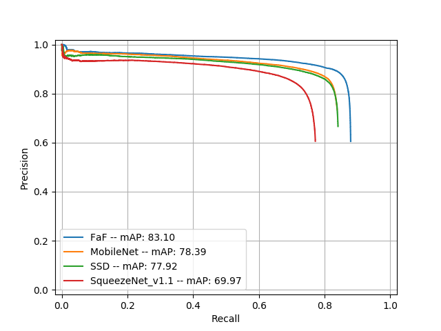
Figure 6: P/R curve

We also report performance as a function of the minimum number of 3D points, which is used to filter ground truth bounding boxes during test time. Note that high level of sparsity is due to occlusion or long distance vehicles. As shown in Fig. 7, our method is able to outperform other methods at all levels. We evaluate with a minimum of 0 point is, to show the importance of exploiting temporal information.

We are also interested in knowing how the model perform as a function of vehicle distance. Towards this goal, we extend the predictions to be as far as 100 meters away. Fig. 8 shows the mAP with IoU 0.7 on vehicles within different distance ranges. We can see that all methods are doing well on nearby vehicles, while our method is significantly better at long range. Note that all methods perform poorly at 100 meters due to lack of 3D points at that distance.

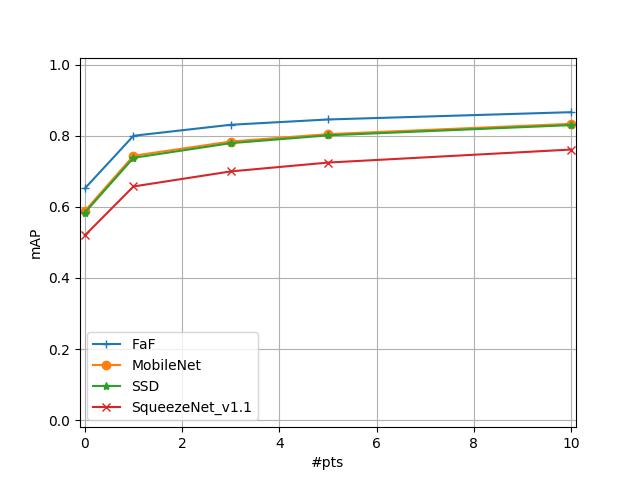
Figure 7: mAP on different number of minimum 3D points

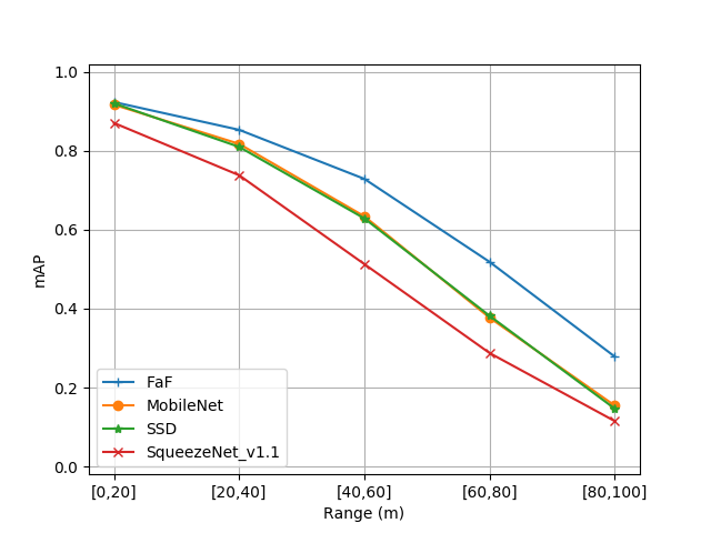
Figure 8: mAP over distance

Single	5 Frames	Early	Laster	w/ F	w/ T	IoU 0.5	IoU 0.6	IoU 0.7	IoU 0.8	IoU 0.9	Time [ms]
✓						89.81	86.27	77.20	52.28	6.33	9
	✓	✓				91.49	88.57	80.90	57.14	8.17	11
	✓		✓			92.01	89.37	82.33	58.77	8.93	29
	✓		✓	✓		92.02	89.34	81.55	58.61	9.62	30
	✓		✓	✓	✓	93.24	90.54	83.10	61.61	11.83	30

Table 2: Ablation study, on $144\times 80$ region with vehicles having $\geq$3 number 3D points

Ablation Study:

We conducted ablation experiments within our framework to show how important each of the component is. We fixed the training setup for all experiments. As shown in Tab. 2, using temporal information with early fusion gives 3.7% improvement on mAP at IoU 0.7. While later fusion uses the same information as early fusion, it is able to get 1.4% extra improvement as it can model more complex temporal features. In addition, adding prediction loss gives similar detection results on current frame alone, however it enables us to decode tracklets and provides evidence to output smoother detections, thus giving the best performance, i.e. 6% points better on mAP at IoU 0.7 than single frame detector.

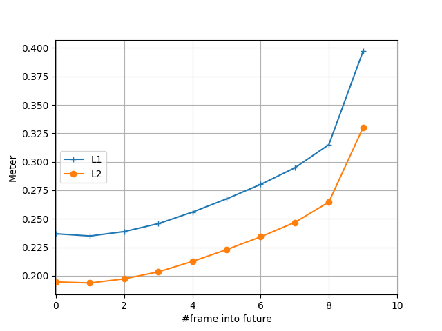
Figure 9: Motion forecasting performance

	MOTA	MOTP	MT	ML
FaF	80.9	85.3	75	10.6
Hungarian	73.1	85.4	55.4	20.8

Table 3: Tracking performance

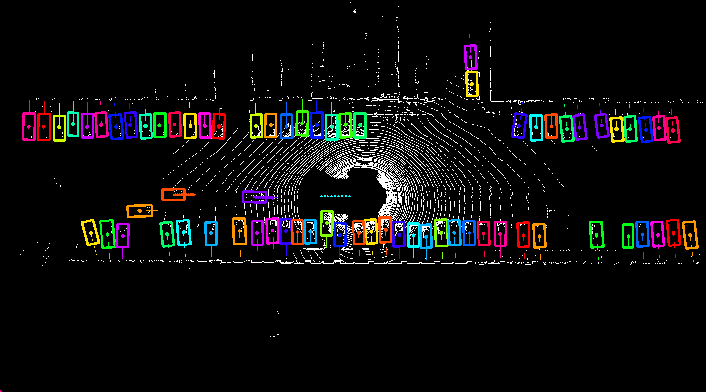
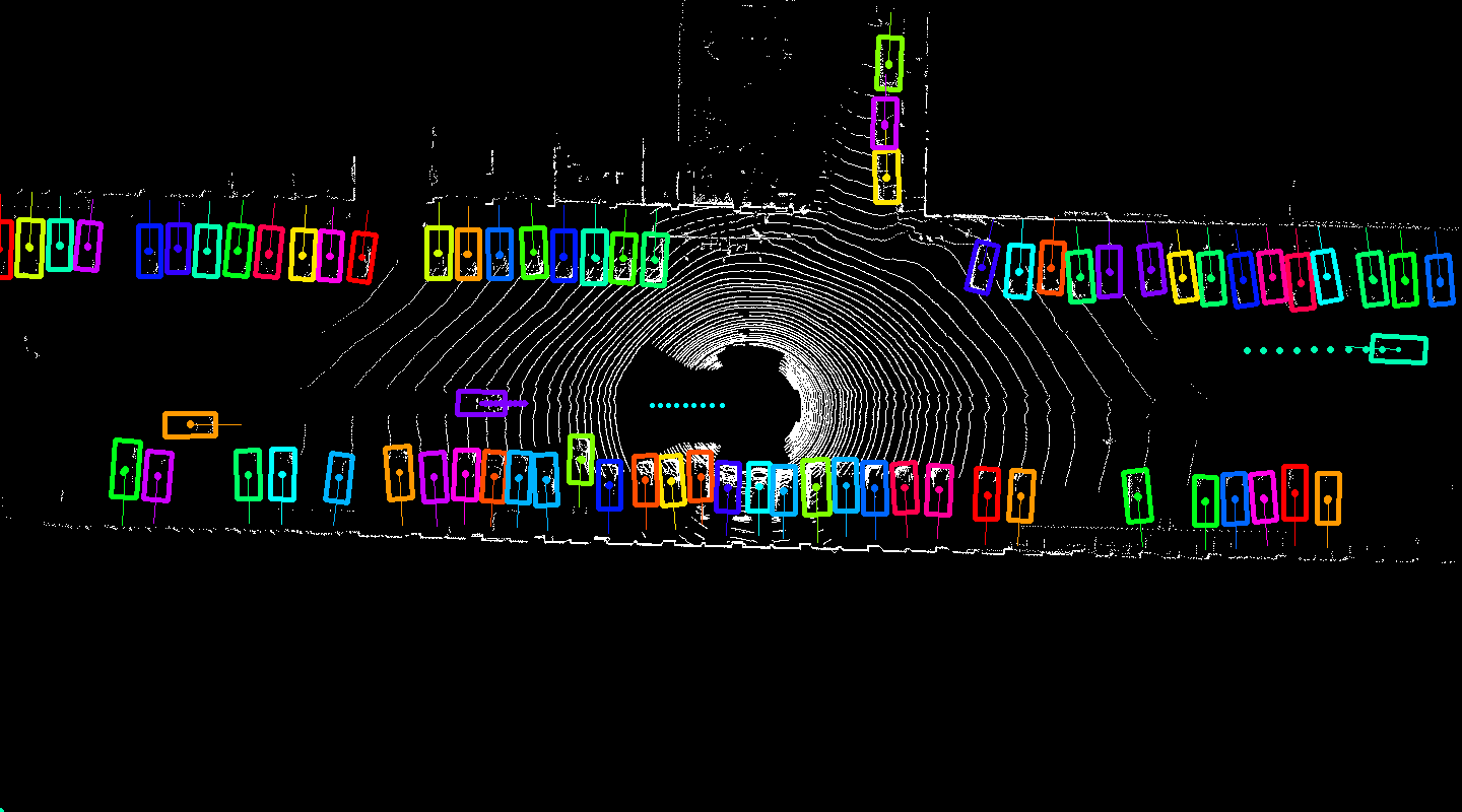
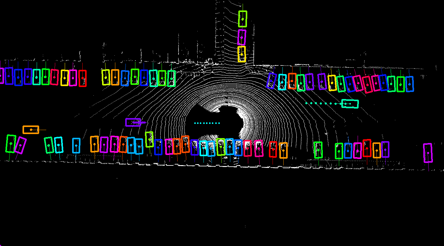
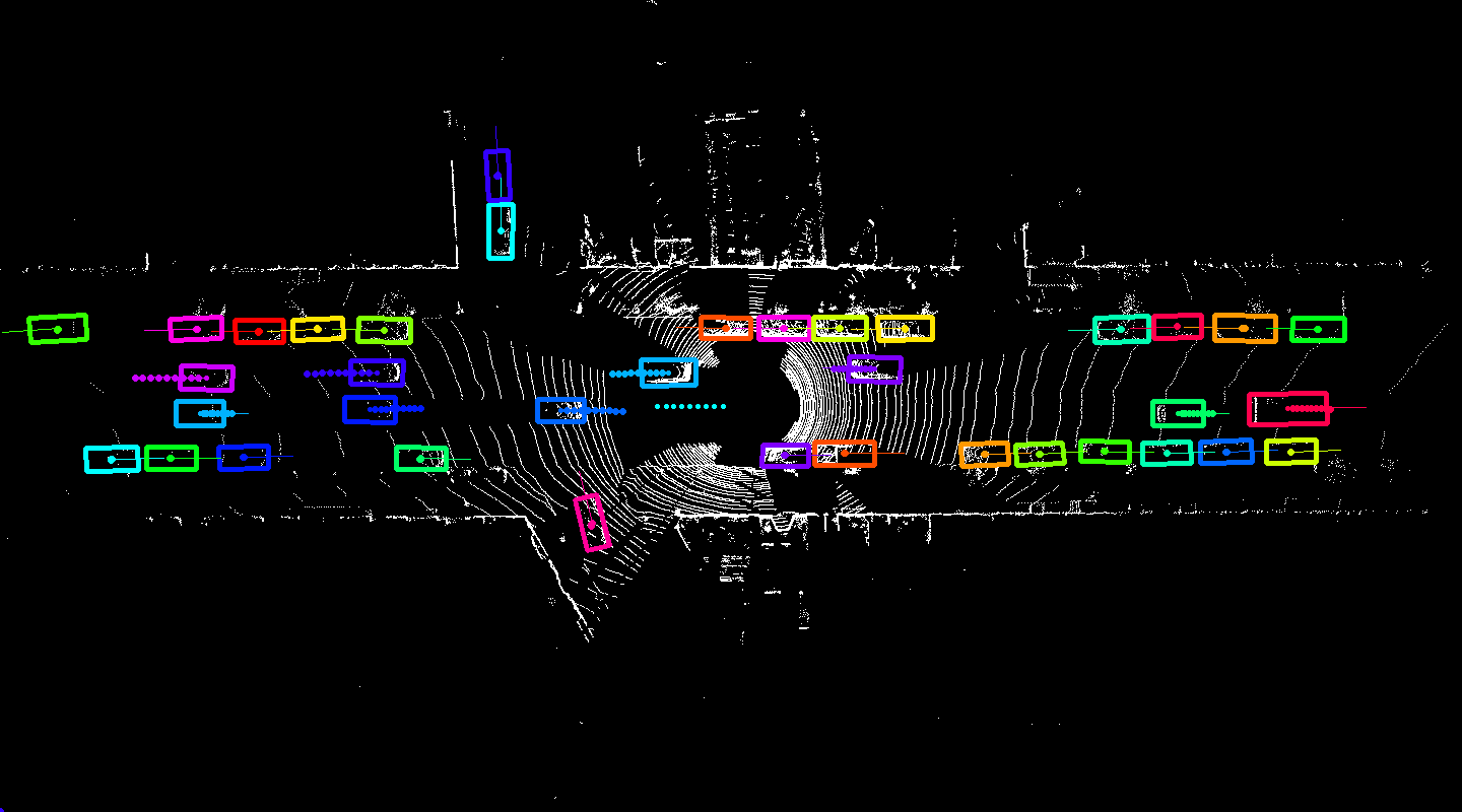
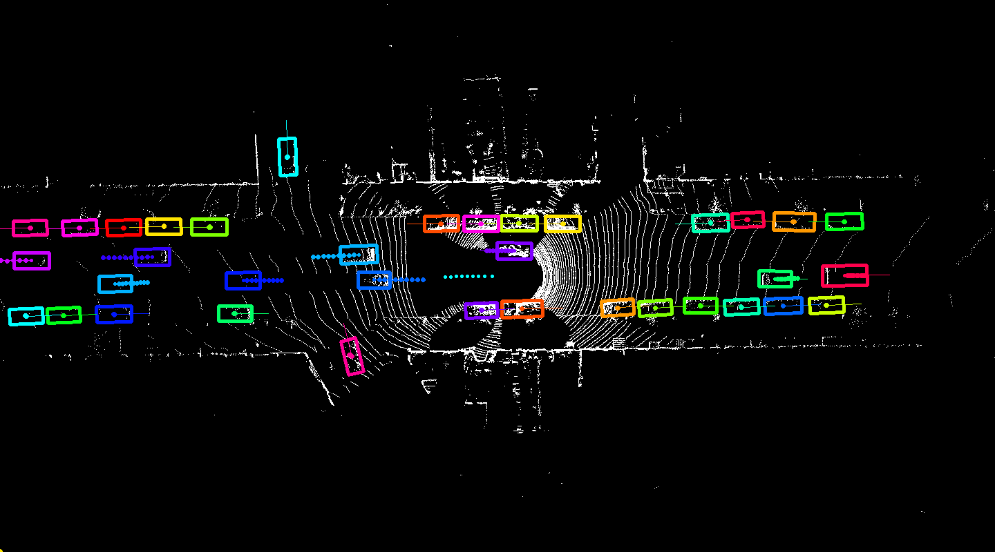
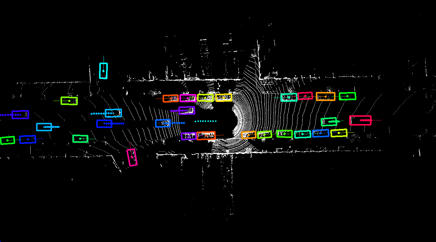
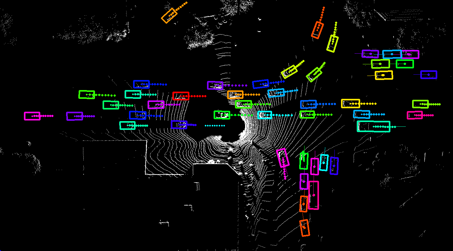
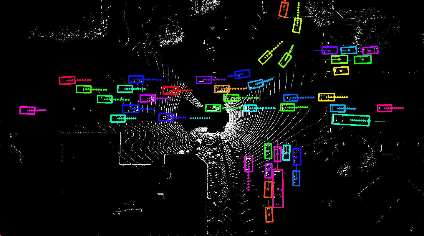
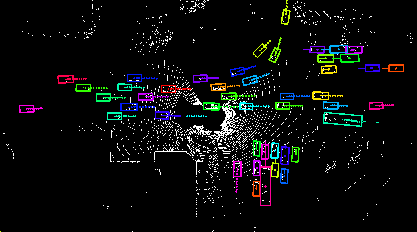
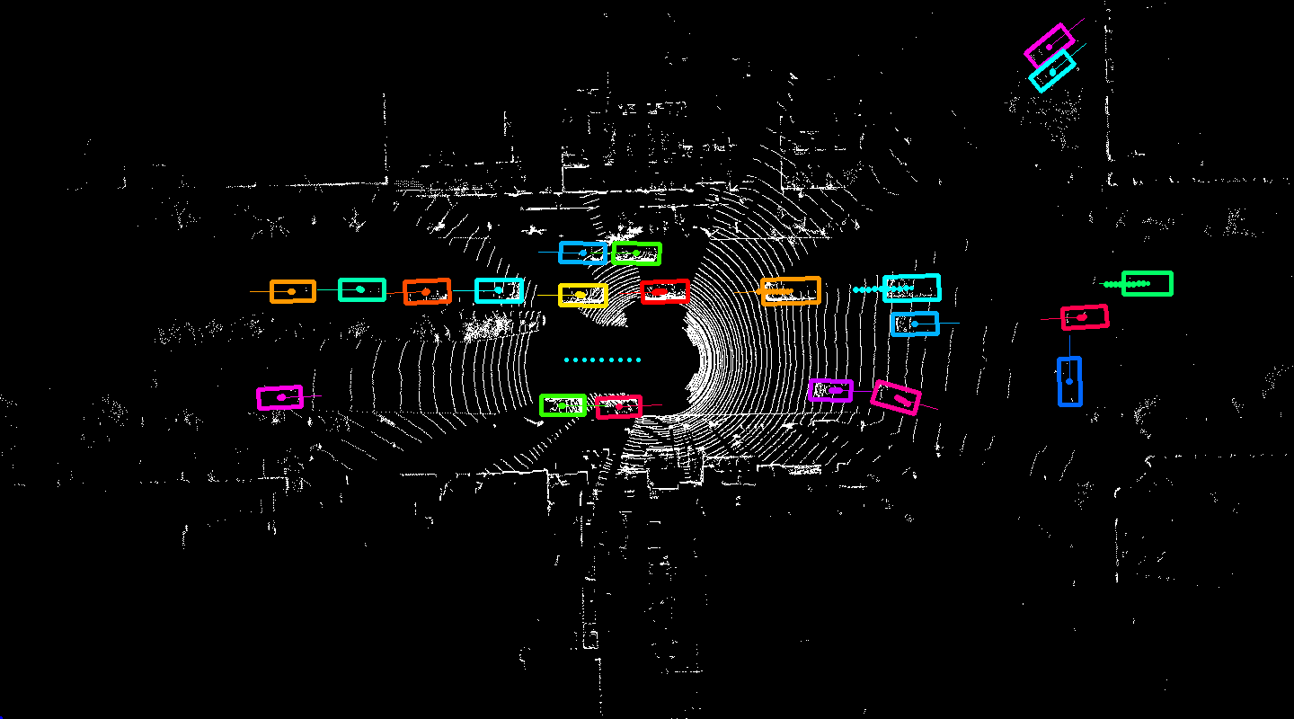
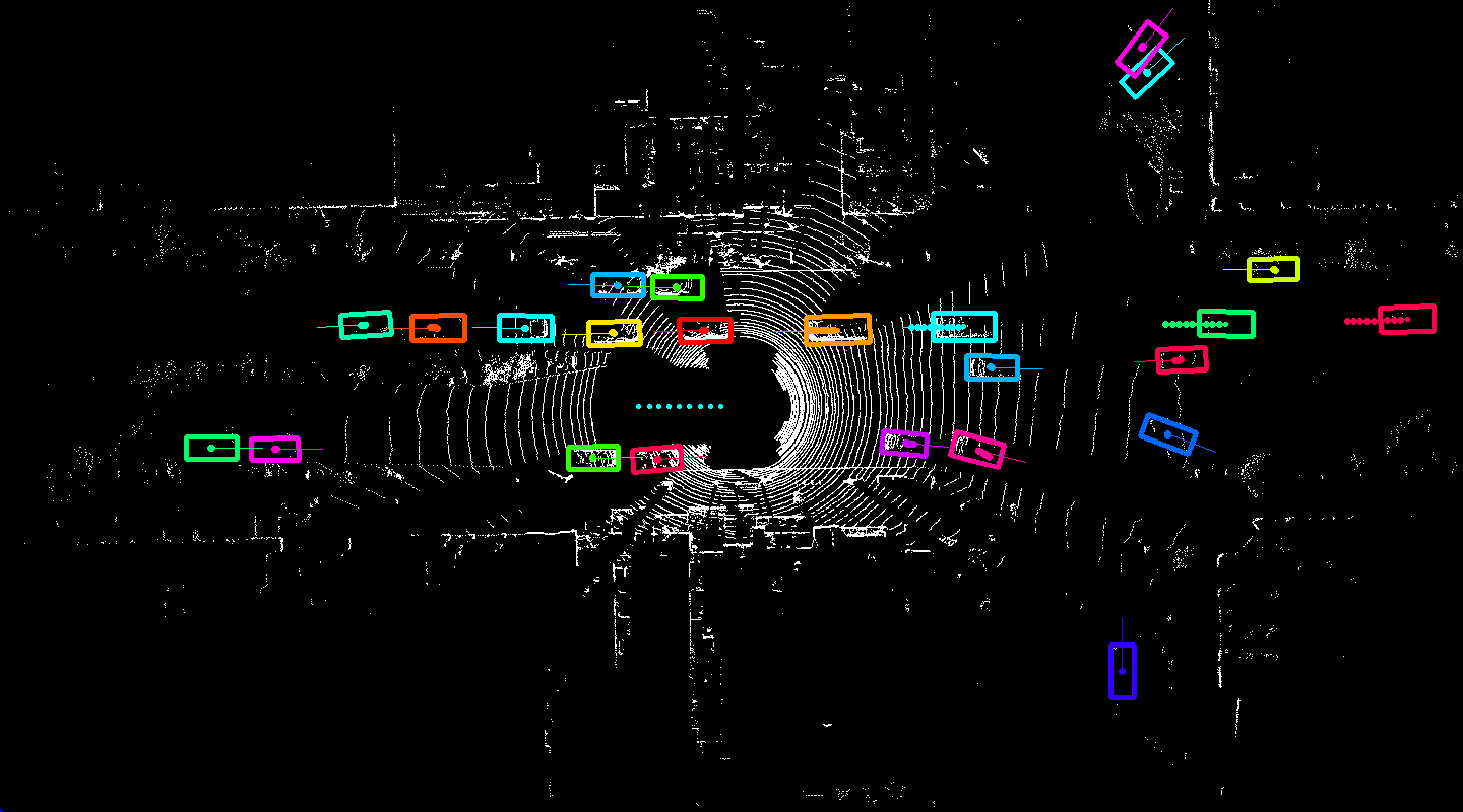
Figure 10: Qualitative results on 144x80M region [best view in color]. Same color represents same vehicle across different timeframe. Each vehicle has ‘dot’ presents the center locations of current and future time frames

Tracking:

Our model is able to output detections with track ids directly. We evaluate the raw tracking output without adding any sophisticated tracking pipeline on top. Tab. 3 shows the comparison between our model’s output and a Hungarian method on top of our detection results. We follow the KITTI protocol [6] and compute MOTA, MOTP, Mostly-Tracked (MT) and Mostly-Lost (ML) across all 100 validation sequences. The evaluation script uses IoU 0.5 for association and 0.9 score for thresholding both methods. We can see that our final output achieves $80.9\%$ in MOTA, $7.8\%$ better than Hungarian, as well as $20\%$ better on MT, $10\%$ lower on ML, while still having similar MOTP.

Motion Forecasting:

We evaluate the forecasting ability of the model by computing the average L1 and L2 distances of the vehicles’ center location. As shown in Fig. 9, we are able to predict 10 frames into the future with L2 distance only less than 0.33 meter. Note that due to the nature of the problem, we can only evaluate on true positives, which in our case has a corresponding recall of $92.5\%$.

Qualitative Results:

Fig. 10 shows our results on a $144\times 80$ meters region. We provide 4 sequences, where the top 3 rows show that our model is able to perform well at complex scenes, giving accurate rotated bounding boxes on both small vehicles as well big trucks. Note that our model also gives accurate motion forecasting for both fast moving vehicles and static vehicles (where all future center locations overlay at the current location). The last row shows one failure case, where our detector fails on the center right blue vehicle. This is due to the sparsity of the 3D points.

5 Conclusion

We have proposed a holistic model that reasons jointly about detection, prediction and tracking in the scenario of autonomous driving. We show that it runs real-time and achieves very good accuracy on all tasks. In the future, we plan to incorporate RoI align in order to have better feature representations. We also plan to test other categories such as pedestrians and produce longer term predictions.

References

- [1] A. Alahi, K. Goel, V. Ramanathan, A. Robicquet, L. Fei-Fei, and S. Savarese. Social lstm: Human trajectory prediction in crowded spaces. In Proceedings of the IEEE Conference on Computer Vision and Pattern Recognition, pages 961–971, 2016.
- [2] X. Chen, K. Kundu, Y. Zhu, H. Ma, S. Fidler, and R. Urtasun. 3d object proposals using stereo imagery for accurate object class detection. IEEE Transactions on Pattern Analysis and Machine Intelligence, 2017.
- [3] X. Chen, H. Ma, J. Wan, B. Li, and T. Xia. Multi-view 3d object detection network for autonomous driving. arXiv preprint arXiv:1611.07759, 2016.
- [4] J. Dai, Y. Li, K. He, and J. Sun. R-fcn: Object detection via region-based fully convolutional networks. In Advances in neural information processing systems, pages 379–387, 2016.
- [5] C. Feichtenhofer, A. Pinz, and A. Zisserman. Detect to track and track to detect. arXiv preprint arXiv:1710.03958, 2017.
- [6] A. Geiger, P. Lenz, and R. Urtasun. Are we ready for autonomous driving? the kitti vision benchmark suite. In Conference on Computer Vision and Pattern Recognition (CVPR), 2012.
- [7] H. Gong, J. Sim, M. Likhachev, and J. Shi. Multi-hypothesis motion planning for visual object tracking. In Computer Vision (ICCV), 2011 IEEE International Conference on, pages 619–626. IEEE, 2011.
- [8] K. He, G. Gkioxari, P. Dollár, and R. Girshick. Mask R-CNN. arXiv preprint arXiv:1703.06870, 2017.
- [9] D. Held, S. Thrun, and S. Savarese. Learning to track at 100 fps with deep regression networks. In European Conference on Computer Vision, pages 749–765. Springer, 2016.
- [10] A. G. Howard, M. Zhu, B. Chen, D. Kalenichenko, W. Wang, T. Weyand, M. Andreetto, and H. Adam. Mobilenets: Efficient convolutional neural networks for mobile vision applications. arXiv preprint arXiv:1704.04861, 2017.
- [11] J. Huang, V. Rathod, C. Sun, M. Zhu, A. Korattikara, A. Fathi, I. Fischer, Z. Wojna, Y. Song, S. Guadarrama, et al. Speed/accuracy trade-offs for modern convolutional object detectors. arXiv preprint arXiv:1611.10012, 2016.
- [12] F. N. Iandola, S. Han, M. W. Moskewicz, K. Ashraf, W. J. Dally, and K. Keutzer. Squeezenet: Alexnet-level accuracy with 50x fewer parameters and¡ 0.5 mb model size. arXiv preprint arXiv:1602.07360, 2016.
- [13] D. Kingma and J. Ba. Adam: A method for stochastic optimization. arXiv preprint arXiv:1412.6980, 2014.
- [14] N. Lee, W. Choi, P. Vernaza, C. B. Choy, P. H. Torr, and M. Chandraker. Desire: Distant future prediction in dynamic scenes with interacting agents. arXiv preprint arXiv:1704.04394, 2017.
- [15] B. Li. 3d fully convolutional network for vehicle detection in point cloud. arXiv preprint arXiv:1611.08069, 2016.
- [16] T.-Y. Lin, P. Goyal, R. Girshick, K. He, and P. Dollár. Focal loss for dense object detection. arXiv preprint arXiv:1708.02002, 2017.
- [17] W. Liu, D. Anguelov, D. Erhan, C. Szegedy, S. Reed, C.-Y. Fu, and A. C. Berg. SSD: Single shot multibox detector. In ECCV, 2016.
- [18] C. Ma, J.-B. Huang, X. Yang, and M.-H. Yang. Hierarchical convolutional features for visual tracking. In Proceedings of the IEEE International Conference on Computer Vision, pages 3074–3082, 2015.
- [19] W.-C. Ma, D.-A. Huang, N. Lee, and K. M. Kitani. Forecasting interactive dynamics of pedestrians with fictitious play. In Proceedings of the IEEE Conference on Computer Vision and Pattern Recognition, pages 774–782, 2017.
- [20] M. Mathieu, C. Couprie, and Y. LeCun. Deep multi-scale video prediction beyond mean square error. arXiv preprint arXiv:1511.05440, 2015.
- [21] H. Nam and B. Han. Learning multi-domain convolutional neural networks for visual tracking. In Proceedings of the IEEE Conference on Computer Vision and Pattern Recognition, pages 4293–4302, 2016.
- [22] S. Pellegrini, A. Ess, K. Schindler, and L. Van Gool. You’ll never walk alone: Modeling social behavior for multi-target tracking. In Computer Vision, 2009 IEEE 12th International Conference on, pages 261–268. IEEE, 2009.
- [23] J. Redmon and A. Farhadi. Yolo9000: better, faster, stronger. arXiv preprint arXiv:1612.08242, 2016.
- [24] S. Ren, K. He, R. Girshick, and J. Sun. Faster R-CNN: Towards real-time object detection with region proposal networks. In Neural Information Processing Systems (NIPS), 2015.
- [25] K. Simonyan and A. Zisserman. Very deep convolutional networks for large-scale image recognition. arXiv preprint arXiv:1409.1556, 2014.
- [26] N. Srivastava, E. Mansimov, and R. Salakhudinov. Unsupervised learning of video representations using lstms. In International Conference on Machine Learning, pages 843–852, 2015.
- [27] R. Tao, E. Gavves, and A. W. Smeulders. Siamese instance search for tracking. In Proceedings of the IEEE Conference on Computer Vision and Pattern Recognition, pages 1420–1429, 2016.
- [28] J. Walker, C. Doersch, A. Gupta, and M. Hebert. An uncertain future: Forecasting from static images using variational autoencoders. In European Conference on Computer Vision, pages 835–851. Springer, 2016.
- [29] L. Wang, W. Ouyang, X. Wang, and H. Lu. Visual tracking with fully convolutional networks. In Proceedings of the IEEE International Conference on Computer Vision, pages 3119–3127, 2015.
- [30] N. Wang and D.-Y. Yeung. Learning a deep compact image representation for visual tracking. In Advances in neural information processing systems, pages 809–817, 2013.
- [31] B. Wu, F. Iandola, P. H. Jin, and K. Keutzer. Squeezedet: Unified, small, low power fully convolutional neural networks for real-time object detection for autonomous driving. arXiv preprint arXiv:1612.01051, 2016.