Comparative Analysis of the Solar Wind: Modeling Charge State Distributions in the Heliosphere

1 Introduction

sec:intro The solar wind is a continuous flow of charged particles emanating from the Sun. The charge states of solar wind plasma provide diagnostic opportunities that can help unravel the mechanisms behind the solar wind acceleration, heating, and origin. Spacecraft such as the Advanced Composition Explorer (ACE), Ulysses (Geiss and Bochsler, 1986), Hinode (Tsuneta, 2006), and the Solar and Heliospheric Observatory (SOHO; Domingo, Fleck, and Poland, 1995) have aided in collecting charge state information to better constrain these complex distribution mechanisms. The continuous data provided by these spacecraft have helped researchers divide the solar wind into two main components, the slow wind ($\sim 300$ km s^-1) and the fast wind ($\sim 750$ km s^-1). Newer spacecraft such as the Parker Solar Probe (Fox et al., 2016) and the Solar Orbiter (Müller et al., 2013) offer modern technologies with incredibly complex instruments that provide an even broader picture of the Sun’s features, especially with the advantages of in situ measurement. In situ charge observations provide sharp constraints on solar wind models. This abundance of observation has driven various theoretical models that seek to explain the solar wind acceleration and heating. Non-equilibrium ionization (NEI) modeling of solar wind plasma is a key strategy for providing constraints on these models.

Time-dependent (or non-equilibrium) ionization becomes relevant when the thermodynamic state of the plasma changes faster than the typical timescales for ionization and recombination. In low-density regions in the solar wind, the plasma is expected to be out of equilibrium because the ionization/recombination time-scales become significantly longer than the dynamic time-scale of plasma. Moreover, the outward moving plasma in the solar wind does not have enough time to reach ionization equilibrium once the density drops significantly below the dense coronal atmosphere at the solar surface. Because of this, the ion species at “freeze-in” in the solar wind can be used to infer the temperature history during solar wind formation as well as place constraints on the solar wind source regions (Dupree, Moore, and Shapiro, 1979; Ko et al., 1997; Owocki and Hundhausen, 1981; Esser and Edgar, 2000). Time-dependent ionization is important for interpreting both remote sensing and in situ observations (e.g., Rakowski, Laming, and Lepri 2007; Landi et al. 2012a). Accounting for non-equilibrium ionization can have a significant difference on the interpretation of the observed structure of the solar atmosphere. By observing spectroscopic line and continuum intensities, one is typically able to use time-dependent ionization as a diagnostic tool to determine the plasma properties and analyse the relevant heating/cooling mechanisms of the plasma. For example, Martínez-Sykora et al. (2016) presented an analysis of the non-equilibrium properties of O³⁺ and Si³⁺ by combining 2D MHD simulations and IRIS’s spectroscopic observations. They looked at the Si IV/O IV line intensities in the quiet Sun and flaring active regions, and found that they were able to reproduce the observed line ratios when they fully considered the non-equilibrium case. Additionally, Kawate et al. (2017) investigated the heating processes of coronal loops in the soft X-ray band to constrain the heating/cooling timescales of hot coronal lines. The emission measure of the coronal loop in the soft X-ray spectra is used to estimate the temperature timescale due to the fact that soft X-ray spectral lines typically correspond to highly ionized particles; and, as a result, Kawate et al. (2017) presented that the line intensities showed a departure from ionization equilibrium where the degree of departure varied depending on the heat inputs for the coronal loop.

In general, the solar wind is not in ionization equilibrium. The electron temperature therefore does not match the local ionic charge state of the solar wind. The fast solar wind is believed to come from the solar coronal holes (Krieger, Timothy, and Roelof, 1973), but pinpointing the source of slower, highly-ionized wind regions remains an active area of research (Abbo et al., 2016). Current theories speculate that they may come from coronal holes with diverging magnetic fields (Wang and Sheeley, 1992; Cranmer, 2009), the tips of helmet streamers (Einaudi et al., 1999; Lapenta and Knoll, 2005), or from interchange reconnection near coronal hole boundaries (Fisk and Schwadron, 2001; Antiochos et al., 2011). A key way to go about exploring the source of the slow solar wind is by examining the inner conditions of the corona through in situ measurements of heavy ions present (Hundhausen, Gilbert, and Bame, 1968; Owocki, Holzer, and Hundhausen, 1983; Gloeckler and Geiss, 2007). Previous studies worked at this by modeling various magnetic field geometries (open or closed) and solar explosions to account for constituents present in the solar wind (Gruesbeck et al., 2011; Landi et al., 2012a, b; Oran et al., 2015; Rodkin et al., 2017). The series of articles produced by Landi et al. (2012a, b, 2014) provide a summary of plasma conditions as the plasma traverses the transition region outward into the fast solar wind. They found that, while the transition region lines were well predicted, the fast wind ionic charge states were underpredicted, indicating that the fast wind streams did not have time to collisionally ionize before departure. They also tested the models of Hansteen and Leer (1995), Cranmer, van Ballegooijen, and Edgar (2007), and Oran et al. (2013). The models were found to be in better agreement with observation when taking the source of the fast solar wind to be from the corona as opposed to the chromosphere. These types of benchmarks are useful for developing and improving upon current theories on the coronal heating and solar wind acceleration problems.

In this paper we analyze the charge state evolution of solar wind plasma that was observed during the Whole Sun Month (WSM, 1996 10 August to 8 September). The WSM was a coordinated observing campaign during Carrington Rotation (CR) 1913 from 1996 August 22 to Sep 18 to characterize and model the solar corona and wind around solar minimum (Galvin and Kohl, 1999; Riley et al., 1999). Solar wind models are heavily dependent on boundary conditions — that is, boundaries involving the magnetic field in the lower corona and conditions surrounding the heliosphere (Aschwanden et al., 2008). We invoked a well developed solar wind model produced by the Magnetohydrodynamics Around a Sphere (MAS) code for the WSM (Linker et al., 1999; Lionello, Linker, and Mikić, 2009) to generate solar wind conditions. We applied the simulated solar wind parameters (temperature, density, velocity, and angular position) to a non-equilibrium ionization code entitled NEI in order to extract ionic information from the stream traces such as the evolution of various charge states and abundance ratios to compare with the quantities observed by the Solar Wind Ion Composition Spectrometer (SWICS; Gloeckler et al., 1983, 1992) (Gloeckler et al., 1992) aboard Ulysses. We analyzed the time-dependent ionization state of plasma until it becomes frozen-in beyond the corona wherein we compare these ionization states with those measured by the SWICS instrument. This approach can ultimately be used to constrain the heating processes of the solar wind by identifying bulk charge states and narrowing down their lower boundary heating mechanisms. Note that with current magnetogram data only being collected from approximately the Earth viewing angle, there is restriction on the observational points which is a known limitation of MHD simulations. Such restrictions can introduce systematic errors in solar wind simulations, but CR 1913 occurred near solar minimum which allowed for a simpler magnetic configuration in the MAS model.

We also focus on the steady outflows above pseudo-streamers, loop-like structures that separate coronal holes of the same polarity (Rachmeler et al., 2014), and relevant NEI effects on the solar wind composition. While MHD models predict accurate wind speeds that motivate the study of turbulence in the heliosphere (Castaing, Gagne, and Hopfinger, 1990; Horbury and Balogh, 1997; Sorriso-Valvo et al., 1999; Pagel and Balogh, 2003; Wawrzaszek et al., 2015; Adhikari et al., 2017), they also allow one to address the fast/slow wind interaction regions (Khabarova et al., 2018; Richardson, 2018).

This paper is organized as follows. In Section sec:data, we describe the acquisition and utilization of the Ulysses data and discuss the MAS model for the Whole Sun Month interval. In Section sec:method, we compare the NEI calculations to SWICS data. In Section sec:results we present our results. In Section sec:discussion, we conclude with a discussion of the relevance of our work.

2 Data Preparation

sec:data The WSM interval was a cumulative modeling and data effort which sought to understand large-scale structures that may persist for several rotations in the solar corona (Galvin and Kohl, 1999). In situ observations contributed to this campaign by providing three-dimensional data out into the interplanetary medium through the observations of spacecraft such as Ulysses. The data we are most interested in are the trace elemental and ionic charge compositions measured by Ulysses/SWICS. During 1996 August 22 to September 18, the Ulysses spacecraft moves from 28$\degree$ to 26$\degree$ heliographic latitude at 4.25 AU from the solar center in the heliographic coordinate system. The main channel SWICS used to analyze and identify the solar wind ions utilized a combination of a time-of-flight sensor, a post-acceleration detector, electrostatic deflection, and residual energy measurement. SWICS was uniquely able to measure both the elemental and ionic charge distributions alongside the mean wind speeds of all of the major solar wind ions (H, He, C, N, O, Ne, Mg, S, Si, and Fe). In our analysis, we assume the abundances of Schmelz, Kimble, and Saba (2012) to calculate theoretical charge states for comparison with SWICS measurements. As mentioned before, measuring the heavy ions in the solar wind is indicative of the plasma conditions in the very early evolution (inner corona) of the solar wind as it travels out into interplanetary space. Moreover, during the WSM campaign Ulysses began sampling increasingly variable wind, a characteristic of the bands of solar wind variability at lower and higher latitudes (Gosling et al., 1997). Having components like the kinetic temperature, mean speeds, and ionic distributions of the heavy ions in the wind gives rise to the underlying physics happening at the solar corona.

We used HelioPy (Stansby, Rai, and Shaw, 2018) to acquire the SWICS data and extract information including the spacecraft coordinates, solar wind velocity and density, and abundance ratios for multiple ions. Once the coordinates of the spacecraft were acquired, we then matched the observation position with the coordinates in the MHD simulation by assuming the kinematics of the plasma were entirely radial. We used the maximum time resolution (3 hr) provided by SWICS for the CR 1913 period for our analysis. This included more than 200 data points starting from September 3 to September 29 (accounting for the 11 days the plasma takes to go from 20 $R_{\odot}$ to Ulysses/SWICS) of detailed constituents of the solar wind at a distance of 4.25 AU. We used all available ions provided by the SWICS database, which included O⁶⁺, C⁶⁺, Ne⁸⁺, Mg¹⁰⁺, Si⁹⁺, S¹⁰⁺, and Fe¹¹⁺. The above plasma and ion properties are used to compared with the following model simulation based on NEI calculation.

A known source of error is that the magnetogram data used as a boundary condition for the far side of the Sun in this simulation is roughly two weeks old. This is particularly relevant because Ulysses was on the opposite side of the Sun from Earth during this period. Comparing the charge states at Ulysses during this interval with those predicted from NEI modeling of the simulation provides a stringent test of the accuracy of this simulation. Riley et al. (1999) performed a similar analysis of comparing charge states between the Sun and Ulysses using two mapping techniques. They compared the results from the commonly used ballistic wind speed approximation with those computed from a two-dimensional inverse MHD algorithm and found that their MHD backwards mapping technique compared more closely to observation. With processes such as rarefaction and compression being possible beyond our MHD modeling boundary, a constant speed approximation might not capture the fast and slow wind stream interactions happening before Ulysses/SWICS samples the wind. Differences between the predicted and observed charge states provide information on how simulations of the solar wind can be improved.

We perform the NEI analysis based on the well-developed coronal MAS model from Predictive Science Inc. (PSI). We analyze a simulation of the Whole Sun Month (WSM) interval that overlapped with CR 1913 from 1996 August 22 to September 18, and obtain the primary plasma variables (velocity, temperature, and density) to apply the NEI calculation. The earlier version of this MHD model has been successfully used to compare the white light polarization emission to Mauna Loa Solar Observatory MK3 images (Linker et al., 1999), and also used to study the pseudo-streamer and helmet streamer during CR 2067 (Abbo et al., 2015). A newer model has been reported by Lionello, Linker, and Mikić (2009), in which they used this model with an improved energy equation to investigate different heating terms in WSM model. The energy equation in the model contains parameterized coronal heating, parallel thermal conduction, radiative losses, and the acceleration of solar wind by Alfvén waves (Lionello, Linker, and Mikić, 2009). The synoptic magnetic field map for the WSM period is obtained from the MDI instrument on SOHO. They made quantitative comparisons with emission in EUV from the EIT instrument on SOHO, and with X-ray emission from the soft X-ray telescope on Yohkoh. In this work, we use the updated model with higher spatial resolution than the Lionello, Linker, and Mikić (2009) model, with $221\times 275\times 431$ grid points, which correspondingly included more small-scale structures in the photospheric magnetic field. This improved MAS model also has been used to analyze NEI properties of a pseudo-streamer during CR 1913 and compare with SOHO/UVCS observations in detail (Shen et al., 2017). In this work, we are interested in the solar wind properties at higher altitudes above this well-studied pseudo-streamer in (Shen et al., 2017), and focus on freeze-in conditions along different trajectories.

3 Method of NEI analysis

sec:method

3.1 Eigenvalue Method

sec: eigenvalue

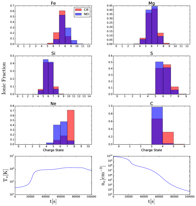
Figure 1.: Shown in these figures are the differences in ion population between a single sample stream trace for the equilibrium (red) and non-equilibrium (blue) cases. These are the modeled charge states at 20 $R_{\odot}$ and with a final velocity of 526 km s^-1. fig: bar˙plots

The ionic charge state of plasma depends on its evolutionary history. We solve the time-dependent ionization equations in Lagrangian form to obtain the charge state by using the Eigenvalue method (Masai, 1984; Hughes and Helfand, 1985; Shen et al., 2015) accompanied by an adaptive time-step that elongates or compresses the time-step depending on plasma conditions in order to retain computational efficiency. The rate of change of the ion population fraction $X_{i}$ for a specific ion with integer charge $i$ is

$$\ilabel{eq:nei_{e}quation}\frac{dX_{i}}{dt}=n_{e}(t)(I_{i-1}X_{i-1}+R_{i}X_{i+1}-I_{i}X_{i}-R_{i-1}X_{i}).$$ (1)

Here, $n_{e}$ is the electron number density. The total ionization and recombination rate coefficients for this ion are $I_{i}$ and $R_{i}$, respectively. These rates were obtained from the CHIANTI version 8.0.7 atomic database (Dere et al., 1997; Landi et al., 2013; Del Zanna et al., 2015; Young et al., 2016). An example of the key differences between collisional ionization equilibrium (CIE) and NEI is shown in Figure (fig: bar_plots). The ionization and recombination rates are functions of the plasma temperature, and do not strongly depend on the density. In a rapidly evolving system where the plasma density and temperature vary with time, the time-dependent ionization equations become non-linear. In individual cases with constant temperature, the evolution of ionic fraction $X_{i}$ tends to its equilibrium state corresponding to this particular temperature. In more general cases, a small time-step is required to accurately capture changes of $X_{i}$ with time. Therefore, we follow the Eigenvalue method to solve time-dependent ionization equations to benefit from its robust and efficient numerical scheme. In summary, the Eigenvalue method takes Eq. (eq: nei_equation) and formulates it into a matrix eigenvalue equation. The key matrix is diagonalizable and comprises all of the ionization and recombination rates for the respective ion. The updated ionization state vector is computed after diagonalizing the matrix of rates and extracting the eigenvalues and matrix of eigenvectors. Mathematically this is formulated as,

$$\ilabel{eq:matrix_{e}q}\frac{d\textbf{F}}{dt}=n_{e}(\hat{\textbf{A}}\cdot\textbf{F}),$$ (2)

where F is the vector containing the ion fractions composed with $Z+1$ ionization levels for an element of atomic number $Z$, and $\hat{\textbf{A}}$ is the matrix containing the ionization and recombination rate coefficients as shown in Eq. (eq: nei_equation). Once one diagonalizes the coefficient matrix $\hat{\textbf{A}}$, the solution of Eq. (eq: matrix_eq) can be written as:

$$\ilabel{eq:eigen_{e}q}\frac{d\textbf{F}^{\prime}}{dt}=n_{e}\hat{\lambda}\cdot\textbf{F}^{\prime},$$ (3)

where $\hat{\lambda}$ is a diagonal matrix containing the eigenvalues calculated from the initial coefficient matrix $\hat{\textbf{A}}$, and $\textbf{F}^{\prime}\equiv\hat{\textbf{V}}^{-1}\textbf{F}$ is the new vector formed by multiplying both sides with a matrix of eigenvectors $\hat{\textbf{V}}$ with eigenvalues $\hat{\lambda}$. In a situation where the plasma temperature is constant and the corresponding ionization and recombination rates are also constant, Eq. (eq: eigen_eq) yields the elementary exponential decay solution: $\textbf{F}^{\prime}=\textbf{F}_{0}$ exp($-n_{e}\hat{\lambda}t$). In this case, F₀ is the initial ion fraction vector for the element in question. The robustness and speed of this method allowed us to compute the ionization balance quite easily and speedily as compared to other numerical schemes like the Runge-Kutta algorithm. Note that this equation is stable even under conditions of very large time-steps which would cause the system to go into a state of equilibrium. We then solve Eq. (eq: nei_equation) using an open source Python project NEI-modeling/NEI and using eigenvalue tables created based on the method reported in Shen et al. (2015).

3.2 Getting the Streamtraces from MAS

sec: streams

In order to solve above ionization equations in a Lagrangian framework, we first trace plasma blobs in the Eulerian framework of MHD simulations, from the solar surface to the top boundary of the MHD model. The coordinate system the Ulysses spacecraft used was the Heliocentric Radial, Tangential, and Normal (HGRTN) system (Fränz and Harper, 2002) which didn’t require any major coordinate transformations in this work because the Heliographic Carrington coordinates match with those used in the MAS model. Since the spacecraft was at a distance of approximately 4 AU and the upper boundary of this MHD model is 20 $R_{\odot}$ from the solar center, we accounted for the time delay of the plasma blob leaving 20 $R_{\odot}$ to reach Ulysses by first averaging out an observed velocity of the instrument from 1996 August 1 to October 1, and then used the mean velocity throughout the WSM interval. This assumption allowed us to arrive at a time delay of 11 days. Due to the Ulysses spacecraft having such a long period of orbit relative to the time-frame of this analysis, we treated it as stationary throughout CR 1913. In doing so, we assumed the bulk outflow speeds measured were purely from the radial component of the MAS model velocity. This assumption was motivated by the velocity contour map produced by the MAS model (see Figure fig: fieldlines). As an effect, we shifted the Ulysses observations 11 days after the WSM interval to allow time for the plasma from CR 1913 to reach the SWICS instrument. Once these shifted dates and coordinates were passed into the MAS model at 20 $R_{\odot}$, it outputted a stream trace corresponding to each Ulysses observational data point. Below 20 $R_{\odot}$, we use ADVECT, a program developed by PSI, to trace the plasma movement using time-dependent velocity fields obtained from the MAS model, and interpolate temperature and density in space and time along each of the tracing trajectories. Thus each stream trace possesses a unique history of temperature, density, velocity, and acceleration.

3.3 Performing NEI Calculations

sec: nei

Once the stream trace data was collected from the MAS model, it was a matter of folding the stream properties through the NEI models. As aforementioned, each stream line possessed various values of temperature, density, and velocity, so an evolutionary charge state distribution from the NEI model had to be calculated for each individual trace. Since the SWICS instrument only tracked the abundant elements in the solar wind — Fe, O, C, Ne, Mg, S, and Si — (Gloeckler et al., 1992), we performed non-equilibrium ionization calculations for all of these elements. The following NEI calculations start from 1.02 $R_{\odot}$ where the plasma number density is usually as high as $10^{10}$ cm^-3 and the plasma is assumed to be in equilibrium ionization states. This allowed us to solve the time-dependent ionization equations and track the charge state distributions for each element present within the plasma traveling up each flux tube out to 20 $R_{\odot}$. The final charge states measured at the end of the simulations were stored for each of the streamers to later be compared to the in situ measurements.

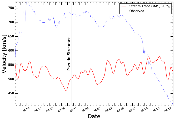
Figure 2.: The compared velocities between the MAS model at 20 $R_{\odot}$ and the mean velocities observed by the Ulysses/SWICS instrument during the Whole Sun Month rotation (CR 1913). The rectangular bar indicates when the outflow produced by the pseudo-streamer would have subtended the observational zone of SWICS.fig: velocity

4 Results

sec:results

Calculating the final charge states meant that we could compare them within situ observations when the charge state is frozen-in already. This meant that, to good approximation, the final plasma state calculated at 20 $R_{\odot}$ consists of the same charge state distributions as expected in the solar wind measured in the outer heliosphere by SWICS. After the calculating the ionization population for each stream trace, we compared the frozen-in plasma with the relative densities (to O⁶⁺) of Si⁹⁺, S¹⁰⁺, Mg¹⁰⁺, Ne⁸⁺, Fe⁸⁺, and C⁶⁺. We also compared the O⁷⁺/O⁶⁺ and C⁶⁺/C⁵⁺ abundance ratios with those found on SWICS.

4.1 Velocity Comparison

sec: v_compare

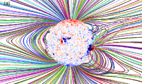
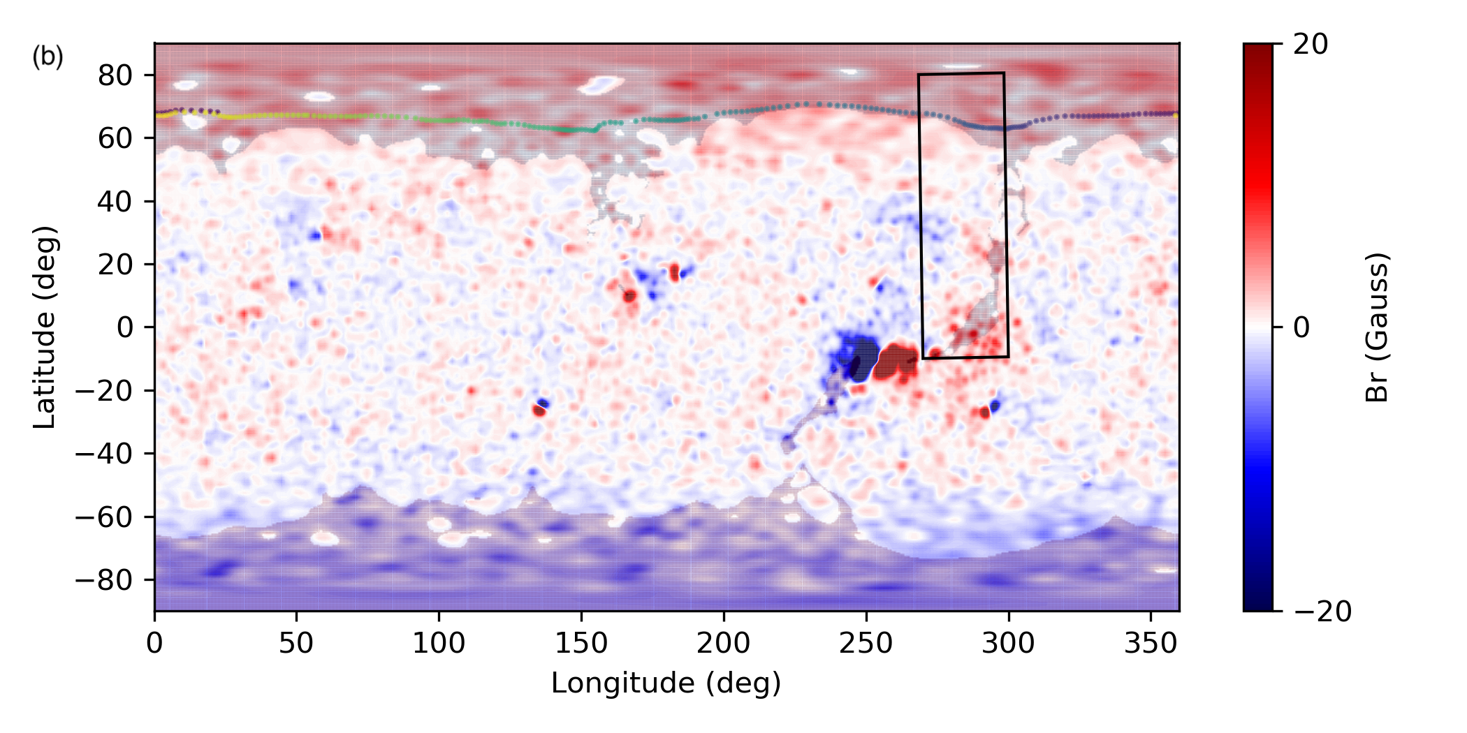
Figure 3.: (a) Magnetic field lines from MAS model for CR 1913; (b) The $B_{r}$ distribution at the solar surface. The dotted lines indicate the rooted position of streamlines at the solar surface and the dark shadow regions are for open field regions. The rectangle shows the pseudo-streamer region fig: fieldlines

The 3D MHD model takes in inputs for the radial magnetic field as a function of colatitude and colongitude governed by available full-Sun magnetogram data and the coronal base temperature and density. The simulation then outputs a range of variables such as the plasma temperature, density, and velocity of the solar wind in steady-state (Aschwanden et al., 2008). By matching the observation dates with CR 1913, we were able to compare winds speeds calculated at the 20 $R_{\odot}$ boundary with those measured by SWICS. Assuming the radial component of the velocity profile in the MAS code dominates, Figure (fig: velocity) shows the bulk flow velocity calculated by the MAS code at the 20 $R_{\odot}$ boundary (solid curve) and compares it with the measured ionic velocities measured by SWICS (dashed curve). The rectangular bar indicates when the pseudo-streamer appeared in the MHD model. The observed velocity profile was the steadiest between the dates of August 23 to September 9. After September 10, the observed wind speed continually declines for the rest of CR 1913. This decline is not captured by the MAS model. Therefore, we will focus the period from August 23 to September 9 in this comparison. We found that the SWICS observation shows a prominence of very fast solar wind (upwards of 700 km s^-1) while the MAS model is computing values in the range of 460 km s^-1 up to 540 km s^-1. This is likely indicative of an acceleration mechanism not accounted for by the MAS model. As a check, we plot the solar magnetic field configuration in Figure (fig: fieldlines) and the observational region (in panel b) shows that the field configuration for the pseudo-streamer greatly changes in the latitudinal direction. A clear feature appearing in both the model and in situ observations is that the velocity profiles show a local minimum plasma speed around this pseudo-streamer except the model-predicted velocity at 20 $R_{\odot}$ is still lower than Ulysses/SWICS measurements at $\sim$ 4 AU which evidences an underpredicted velocity profile by the MHD model. Another possibility is that there is acceleration beyond 20 $R_{\odot}$. The fact of highly-ionized plasma occupying slow solar wind streams is also confirmed by our analyses, but again the MHD wind speeds do not agree with the in situ measurements of SWICS.

In MHD modeling cases where the plasma is leaving the corona slower than in reality, the plasma will have more time for the charge states to evolve. The observed charge states could have frozen in at higher heights. For example, if the plasma is dropping in temperature as it moves away from the Sun, the charge states may correspond to lower temperatures than observed by Ulysses. This may contribute as one of the sources of errors in the following comparison between NEI calculations and Ulysses/SWICS observations.

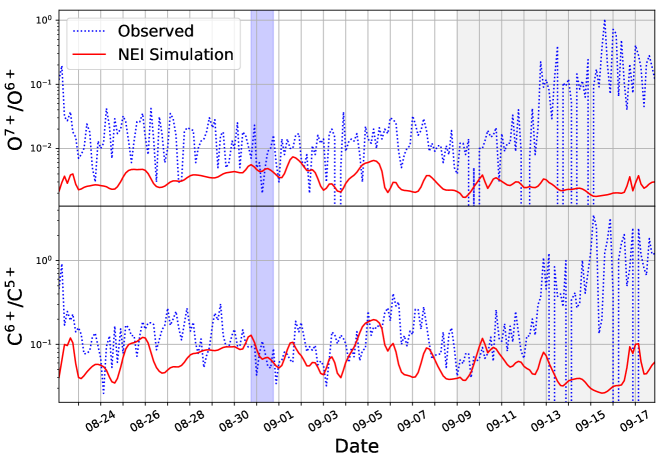
Figure 4.: The abundance ratios of solar wind ions measured by the SWICS instrument compared with the calculated values of our NEI model along with the labeled appearance of the pseudo-streamer. The grey area indicates where SWICS began to observe a decline in solar wind velocity which agrees with the anti-correlated nature of high ionization in the slower wind streams. fig: abund

4.2 Charge State and Abundance Ratio Comparison

sec: abund_compare

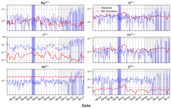
Figure 5.: The ionic densities relative to O⁶⁺ for the main solar wind ions measured by SWICS. The observation (blue) is superimposed with the model (red) where the model is in reasonable agreement for a few of the ions in question. The blue rectangle indicates the pseudo-streamer observation. fig: density

In this section, we calculated the final non-equilibrium ionic fractions at the 20 $R_{\odot}$ boundary based on temperature and density values predicted by the MAS model. We used ionization/recombination tables assuming the Maxwellian distribution throughout the NEI simulation. Although non-Maxwellian electron distribution functions exist in the ion-forming region (Esser et al., 2003), we assume these effects to be negligible in reference to our calculations. The O⁷⁺/O⁶⁺ and C⁶⁺/C⁵⁺ ratios measured by the SWICS instrument were compared with the results of the NEI simulation. Observed in situ abundance ratios are shown in Figure (fig: abund) where we have superimposed the NEI calculated fractions on top of the SWICS measurements. The blue strip indicates when the pseudo-streamer outflow would have made it to SWICS, and the grey region indicates the start of the decline in observed solar wind speed as seen in Figure (fig: velocity). Figure (fig: density) shows the relative densities of each measured ion versus the NEI calculated ratios. The simulation lies within reasonable agreement for the Fe¹¹⁺, Mg¹⁰⁺, Si⁹⁺, but does not match well with the other ions in question. An interesting observation is that the region of solar wind decline is highly correlated to a higher degree of ionization for all observed solar wind ions which would suggest an increase in temperature and magnetic field strength, but Figure (fig: mag) contradicts that notion. The O⁷⁺/O⁶⁺ ratio is a proxy for the degree of ionization in solar plasma, and the observed ratio increase towards the end of the WSM (Figure fig: abund) might be attributed to the plasma having more time to ionize as it moved away from the Sun.

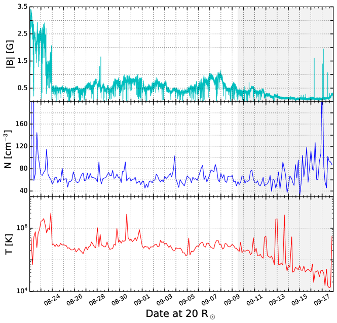
Figure 6.: Shown above are the magnetometer data, $\alpha$-particle density, and $\alpha$-particle temperature measured by SWICS. The grey region indicates when the observed winds begin to decelerate. This important distinction is made for the peculiar result shown in Figure (fig: abund) .fig: mag

4.3 Charge State Freeze-In Heights

sec: freeze_heights In wanting to understand the heavy ion distribution in reference to their expansion into the solar wind, we measured the “freeze-in” heights of each solar wind ion from the model prediction.

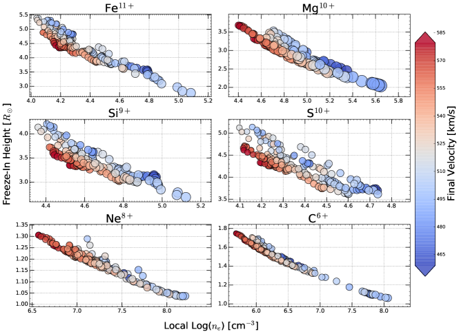
Figure 7.: Freeze-in heights obtained from the MHD model for the respective streamline traces corresponding to Ulysses/SWICS observational data points. The horizontal-axis indicates the local density when a particular ion freezed in, and the color indicates the final plasma flow velocity at 20$R_{\odot}$. fig: heights

Measurements of the ions at freeze-in potentially yield information about the solar plasma conditions at the coronal base (Owocki, Holzer, and Hundhausen, 1983). For each position corresponding to the date of Ulysses/SWICS observations, we monitored the constant NEI states along each streamline and found the freeze-in height for each ion. Figure (fig: heights) shows the heights at which each ion’s ionization state becomes fixed with respect to both the final velocity at 20 $R_{\odot}$ and the local freeze-in density along the flux tube. We can see a trend of ions freezing in at higher heights based on the magnitude of their velocity profiles. This corresponds to the fact that plasma that is moving quickly from the solar surface takes comparatively longer to equilibrate. It is also clear that freeze-in heights dramatically drop as the local density increases because the ionization/recombination time-scales become short in dense plasma environments. For relatively low-temperature ions, such as C⁶⁺ and Ne${{}^{8}+}$, the ions generally freeze-in lower altitudes (1.8 and 1.3$R_{\odot}$) even for the high speed flows with velocity up to ${\sim}$ 600 km s^-1. On the other hand, the high-temperature ions (Si⁹⁺, S¹⁰⁺, Fe¹¹⁺) show much wider freeze-in height ranges depending on the flow speed. Along with the freeze-in heights-density profiles in Figure (fig: heights), we noticed that our analysis does not show the higher density ranges ($>{10^{6}}$ cm^-3) for Fe¹¹⁺ due to the limited sampling points from the current MHD model. It will be interesting to investigate the freeze-in heights in more dense plasma cases in the future. Moreover, we have included the freeze-in heights for Fe¹⁰⁺ and Fe¹³⁺ in one figure (Figure fig: iron_freeze_in) to discuss the variation of freeze-in heights with charge states. The overall feature of Figure fig: iron_freeze_in is that Fe¹⁰⁺ ions freeze in at lower heights first, and Fe¹³⁺ fraction becomes fixed at the higher altitudes. This tendency is consistent with recently solar wind observations (e.g., Boe et al., 2018). Boe et al. (2018) provided reliable measurements for the freeze-in heights of the aforementioned ions for coronal holes. They measured the freeze-in distances to be in the range of 1.4 to 2 $R_{\odot}$ for Fe¹⁰⁺ and from 1.5 to 2.2 $R_{\odot}$ for Fe¹³⁺ in open field streamer regions during the 2015 March 20 total solar eclipse. In here, we compute a wider range of freeze-in heights in our model, showing how the dynamics of different coronal features can greatly affect when and where ionization states become fixed. Note that in the right corner of the Fe¹⁰⁺ panel in Figure (fig: iron_freeze_in), the freeze-in heights match closely to those found in Boe et al. (2018) while the Fe¹³⁺ distances are a bit higher partly due to the absence of higher density sampling streamlines from the current MHD model.

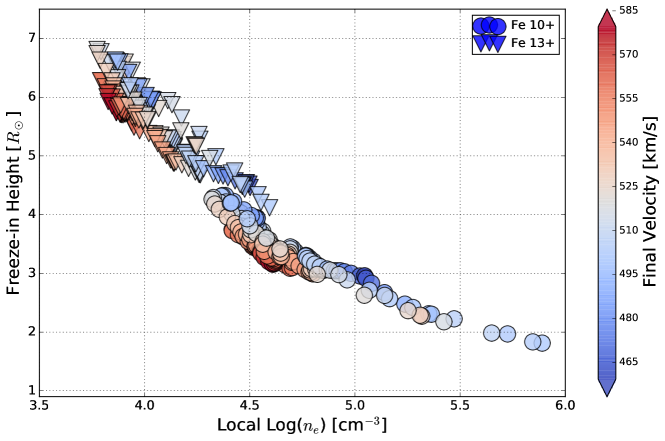
Figure 8.: The freeze-in distances vary with local density and final plasma flow speed for Fe¹⁰⁺ and Fe¹³⁺ ions calculated from the MHD model. The sampling points are chosen to be the same as in Figure fig: heights. fig: iron˙freeze˙in

Overall, the ion density to freeze-in height relationship corresponds well with the notion that local density falls with the height. Additionally, Figures(fig: heights & fig: iron_freeze_in) both show that faster moving ions freeze in at higher heights. What is not fully understood is the order-of-magnitude differences between the local densities. Nonetheless, these results are useful for one seeking to provide constraints on freeze-in distances and local densities given the outflow velocities of a wind near the northern edge variability band as described in Gosling et al. (1997). For instance, one looking to estimate the freeze-in distance for Mg¹⁰⁺ that is moving at a velocity greater than 570 km s^-1 can expect to see the ionization state become fixed beyond a distance of 3.5 $R_{\odot}$.

5 Summary

sec:discussion In this analysis, we used NEI calculations to compare model predicted charge state populations with those observed by the Ulysses/SWICS instrument during the WSM interval CR 1913 (1996 August 22 to September 18). We calculated charge states of abundant elements in solar wind by using the plasma evolution obtained from the MAS model up to 20 $R_{\odot}$. We then assume a steady velocity thereafter until the plasma reaches the SWICS instrument located at about 4.25 AU during this WSM interval. We compared the modeling plasma velocity at 20 $R_{\odot}$ versus the bulk flow velocities measured by Ulysses/SWICS. The discrepancies shown in Figure (fig: velocity) might be attributed to the MHD model not accounting for acceleration within 20$R_{\odot}$ or that the plasma accelerates beyond the modeling boundary. For a discussion of solar wind acceleration mechanisms beyond 20 $R_{\odot}$, we refer the reader to work such as those by McGregor et al. (2011).

We compared densities (relative to O⁶⁺) of the SWICS ions (C, O, Ne, Mg, S, Si, Fe) with our NEI calculations and found that Fe¹¹⁺, Mg¹⁰⁺, and Si⁹⁺ ratios matched observation much better than S¹⁰⁺, Ne⁸⁺, and C⁶⁺. We then measured the modeled O⁷⁺/O⁶⁺ and C⁶⁺/C⁵⁺ ratios with the in situ measurements and found reasonable agreement up until the drastic change in ion population that we assume was due to the interaction region ionizing the plasma beyond 20 $R_{\odot}$. To check for any sign of solar energetic events, we plotted the observed magnetic field strength, $\alpha$-particle density, and temperature in Figure (fig: mag). We might infer that the abrupt changes in these characteristics starting from the grey region in the plot provide more evidence of a heliospheric shift in the plasma conditions that was not captured by the MHD simulation. The velocity profile transitioning to the slow wind regime implies a mixing of plasma domains (Pizzo and Gosling, 1994; Gosling et al., 1997; Gosling and Pizzo, 1999) that might explain the large discrepancy between our model and observations. To be certain, we searched all available data for signs of solar energetic events during this WSM interval to no avail. In such a search, one might check for the presence a high-energy event via the Large Angle and Spectrometric Coronagraph (LASCO) aboard SOHO, but no such event was present in the data.

We calculated the freeze-in heights — the point at which ionization temperature is constant — for ions while relating this quantity to both the local plasma density at freeze-in as well as the plasma final velocity at 20$R_{\odot}$. This method can potentially be useful for observers wanting to know reference values for particular ions given initial conditions of the plasma. The results we found for Fe¹⁰⁺ and Fe¹³⁺ offer a wider range of freeze-in values than those reported by Boe et al. (2018). Our calculated freeze-in heights ranges for Fe¹⁰⁺ (4.5 to 7.5 $R_{\odot}$) and Fe ¹³⁺ (4.0 to 7.0 $R_{\odot}$) were greater than the combined ranges for both Fe¹⁰⁺ (1.4 to 2 $R_{\odot}$) and Fe¹³⁺ (1.5 to 2.2 $R_{\odot}$) examined in the Boe et al. (2018) work — with the effects of systematic error taken into account — but we emphasize that this discrepancy can be attributed to a wide range of uncertainties in MHD simulations, such as inaccurate acceleration within 20$R_{\odot}$. It is also likely to be an inherent fundamental difference between the magnetic field regions at which our two observations occur. Although under different magnetic field configurations, we cite the work of Boe et al. (2018) for comparison as a means of demonstrating the curious physical effects at play between different streamer regions. Future studies could shine more light on how impactful both coronal and ambient magnetic field configurations affect the freeze-in distance for many solar wind ions.

NEI calculations are highly sensitive to electron density and temperature evolutionary history. Differences between the true solar wind velocity and the velocity given by the simulation will contribute to discrepancies between the predicted and observed charge state distributions. Although the discrepancy of ion populations between observations and models in the past have been hypothesized to be due to non-thermal electrons (Esser et al., 2003), the differences between non-Maxwellian versus Maxwellian distributions in terms of the degree of ionization in the solar wind are negligibly small (Laming and Lepri, 2007). This is worth exploring in the future. Since the simulation domain of this MHD model is up to 20 $R_{\odot}$, it cannot reveal the plasma movement and directly obtain the velocity prediction at Ulysses’ orbit. Note that our driving assumption throughout this procedure was that the plasma velocity remains constant from 20 $R_{\odot}$ onward. The error in not accounting for acceleration beyond the 20 $R_{\odot}$ boundary is beyond the scope of this paper. It is possible that the solar wind accelerated in the interplanetary medium by means of wave-particle interactions such as shocks, but signs of shock-producing events such as coronal mass ejections (CMEs) were not detected by available coronagraphs. However, the model’s velocity profile provides sufficient information on the plasma before acceleration.

In essence, the variation in solar wind speed can come from a variety of sources and tracing a parcel of plasma back to the source is quite difficult at 1 AU let alone 4 AU. Future work would be to implement different electron distributions in the NEI model such as the kappa distribution which accounts for non-Maxwellian suprathermal tails. Velocity calculations in the MAS code may also be an important step towards improving the NEI models since they rely so heavily on the magnetic field configuration. The large discrepancy between the observed velocity profile in the MAS model tells us that either the MHD code is largely underestimating the velocity of the plasma outflow, we were incorrect in assuming the velocity was purely radially outward at the 20 $R_{\odot}$ boundary, or a combination of both effects. A more sophisticated approach of back tracing a plasma flow from 4 AU to the Sun would be to use an inverse MHD mapping as discussed in Riley et al. (1999). This way, the plasma parcel is accounted for throughout its entire journey and the appropriate acceleration mechanisms can be properly assessed throughout the trajectories. We acknowledge that in our report there are systematic errors that might have produced the differing effects, but such errors are not easily quantifiable. One way to smooth the systematic error in future work would be to expand our observation region to account for solar latitudes that might match more closely to observation.

This work was primarily supported by NSF SHINE Grant AGS-1723313 to the Smithsonian Astrophysical Observatory (SAO) and a Smithsonian Institution Scholarly Studies grant. C.S. is supported by NSF grant AST-1735525, and NASA grants 80NSSC20K1318, 80NSSC19K0853, and 80NSSC18K1129 to SAO. N.M. acknowledges partial support by NSF grant 1931388, NASA grants 80NSSC19K0853 and 80NSSC20K0174, and NASA contract NNM07AB07C to SAO.

Facilities: Ulysses, SOHO

Software: MAS, NEI (Shen, Raymond, and Murphy, 2015), HelioPy (Stansby, Rai, and Shaw, 2018), Astropy (Astropy Collaboration et al., 2018), PlasmaPy (PlasmaPy Community et al., 2018a, b), CHIANTI, v8.0.7, is a collaborative project involving George Mason University, the University of Michigan (USA), University of Cambridge (UK) and NASA Goddard Space Flight Center (USA).

Acknowledgments

The authors acknowledge helpful discussions with W. Barnes, J. Raymond, K. Reeves, D. Stansby and M. Stevens; and thank PSI for providing the MAS simulation.

References

- Abbo et al. (2015) Abbo, L., Lionello, R., Riley, P., Wang, Y.-M.: 2015, Coronal Pseudo-Streamer and Bipolar Streamer Observed by SOHO/UVCS in March 2008. Sol. Phys. 290, 2043. DOI.
- Abbo et al. (2016) Abbo, L., Ofman, L., Antiochos, S.K., Hansteen, V.H., Harra, L., Ko, Y.-K., Lapenta, G., Li, B., Riley, P., Strachan, L., von Steiger, R., Wang, Y.-M.: 2016, Slow Solar Wind: Observations and Modeling. Space Sci. Rev. 201(1-4), 55. DOI.
- Adhikari et al. (2017) Adhikari, L., Zank, G.P., Hunana, P., Shiota, D., Bruno, R., Telloni, D.: 2017, Evolution of Power Anisotropy in Magnetic Field Fluctuations Throughout the Heliosphere. In: AGU Fall Meeting Abstracts 2017, SH33B.
- Antiochos et al. (2011) Antiochos, S.K., Mikić, Z., Titov, V.S., Lionello, R., Linker, J.A.: 2011, A Model for the Sources of the Slow Solar Wind. ApJ 731(2), 112. DOI.
- Aschwanden et al. (2008) Aschwanden, M.J., Burlaga, L.F., Kaiser, M.L., Ng, C.K., Reames, D.V., Reiner, M.J., Gombosi, T.I., Lugaz, N., Manchester, W., Roussev, I.I., Zurbuchen, T.H., Farrugia, C.J., Galvin, A.B., Lee, M.A., Linker, J.A., Mikić, Z., Riley, P., Alexander, D., Sandman, A.W., Cook, J.W., Howard, R.A., Odstrčil, D., Pizzo, V.J., Kóta, J., Liewer, P.C., Luhmann, J.G., Inhester, B., Schwenn, R.W., Solanki, S.K., Vasyliunas, V.M., Wiegelmann, T., Blush, L., Bochsler, P., Cairns, I.H., Robinson, P.A., Bothmer, V., Kecskemety, K., Llebaria, A., Maksimovic, M., Scholer, M., Wimmer-Schweingruber, R.F.: 2008, Theoretical modeling for the stereo mission. Space Sci. Rev. 136, 565. DOI.
- Astropy Collaboration et al. (2018) Astropy Collaboration, Price-Whelan, A.M., Sipőcz, B.M., Günther, H.M., Lim, P.L., Crawford, S.M., Conseil, S., Shupe, D.L., Craig, M.W., Dencheva, N., Ginsburg, A., VanderPlas, J.T., Bradley, L.D., Pérez-Suárez, D., de Val-Borro, M., Aldcroft, T.L., Cruz, K.L., Robitaille, T.P., Tollerud, E.J., Ardelean, C., Babej, T., Bach, Y.P., Bachetti, M., Bakanov, A.V., Bamford, S.P., Barentsen, G., Barmby, P., Baumbach, A., Berry, K.L., Biscani, F., Boquien, M., Bostroem, K.A., Bouma, L.G., Brammer, G.B., Bray, E.M., Breytenbach, H., Buddelmeijer, H., Burke, D.J., Calderone, G., Cano Rodríguez, J.L., Cara, M., Cardoso, J.V.M., Cheedella, S., Copin, Y., Corrales, L., Crichton, D., D’Avella, D., Deil, C., Depagne, É., Dietrich, J.P., Donath, A., Droettboom, M., Earl, N., Erben, T., Fabbro, S., Ferreira, L.A., Finethy, T., Fox, R.T., Garrison, L.H., Gibbons, S.L.J., Goldstein, D.A., Gommers, R., Greco, J.P., Greenfield, P., Groener, A.M., Grollier, F., Hagen, A., Hirst, P., Homeier, D., Horton, A.J., Hosseinzadeh, G., Hu, L., Hunkeler, J.S., Ivezić, Ž., Jain, A., Jenness, T., Kanarek, G., Kendrew, S., Kern, N.S., Kerzendorf, W.E., Khvalko, A., King, J., Kirkby, D., Kulkarni, A.M., Kumar, A., Lee, A., Lenz, D., Littlefair, S.P., Ma, Z., Macleod, D.M., Mastropietro, M., McCully, C., Montagnac, S., Morris, B.M., Mueller, M., Mumford, S.J., Muna, D., Murphy, N.A., Nelson, S., Nguyen, G.H., Ninan, J.P., Nöthe, M., Ogaz, S., Oh, S., Parejko, J.K., Parley, N., Pascual, S., Patil, R., Patil, A.A., Plunkett, A.L., Prochaska, J.X., Rastogi, T., Reddy Janga, V., Sabater, J., Sakurikar, P., Seifert, M., Sherbert, L.E., Sherwood-Taylor, H., Shih, A.Y., Sick, J., Silbiger, M.T., Singanamalla, S., Singer, L.P., Sladen, P.H., Sooley, K.A., Sornarajah, S., Streicher, O., Teuben, P., Thomas, S.W., Tremblay, G.R., Turner, J.E.H., Terrón, V., van Kerkwijk, M.H., de la Vega, A., Watkins, L.L., Weaver, B.A., Whitmore, J.B., Woillez, J., Zabalza, V., Astropy Contributors: 2018, The Astropy Project: Building an Open-science Project and Status of the v2.0 Core Package. AJ 156, 123. DOI.
- Boe et al. (2018) Boe, B., Habbal, S., Druckmüller, M., Landi, E., Kourkchi, E., Ding, A., Starha, P., Hutton, J.: 2018, The First Empirical Determination of the Fe10+ and Fe13+ Freeze-in Distances in the Solar Corona. ApJ 859, 155. DOI.
- Castaing, Gagne, and Hopfinger (1990) Castaing, B., Gagne, Y., Hopfinger, E.J.: 1990, Velocity probability density functions of high Reynolds number turbulence. Physica D Nonlinear Phenomena 46(2), 177. DOI.
- Cranmer (2009) Cranmer, S.R.: 2009, Coronal Holes. Living Reviews in Solar Physics 6(1), 3. DOI.
- Cranmer, van Ballegooijen, and Edgar (2007) Cranmer, S.R., van Ballegooijen, A.A., Edgar, R.J.: 2007, Self-consistent Coronal Heating and Solar Wind Acceleration from Anisotropic Magnetohydrodynamic Turbulence. Astrophys. J. Supp. Ser. 171(2), 520. DOI.
- Del Zanna et al. (2015) Del Zanna, G., Dere, K.P., Young, P.R., Landi, E., Mason, H.E.: 2015, CHIANTI - An atomic database for emission lines. Version 8. A&A 582, A56. DOI.
- Dere et al. (1997) Dere, K.P., Landi, E., Mason, H.E., Monsignori Fossi, B.C., Young, P.R.: 1997, CHIANTI - an atomic database for emission lines. Astronomy and Astrophysics Supplement Series 125, 149. DOI.
- Domingo, Fleck, and Poland (1995) Domingo, V., Fleck, B., Poland, A.I.: 1995, SOHO: The Solar and Heliospheric Observatory. Space Sci. Rev. 72(1-2), 81. DOI.
- Dupree, Moore, and Shapiro (1979) Dupree, A.K., Moore, R.T., Shapiro, P.R.: 1979, Nonequilibrium ionization in solar and stellar winds. ApJ 229, L101. DOI.
- Einaudi et al. (1999) Einaudi, G., Boncinelli, P., Dahlburg, R.B., Karpen, J.T.: 1999, Formation of the slow solar wind in a coronal streamer. J. Geophys. Res. 104(A1), 521. DOI.
- Esser and Edgar (2000) Esser, R., Edgar, R.J.: 2000, Reconciling Spectroscopic Electron Temperature Measurements in the Solar Corona with In Situ Charge State Observations. ApJ 532, L71. DOI.
- Esser et al. (2003) Esser, R., Lie-Svendsen, Ø., Edgar, R., Chen, Y.: 2003, Observational and theoretical constraints on the heating and acceleration of the fast solar wind. In: Solar Wind Ten 679, 249. DOI.
- Fisk and Schwadron (2001) Fisk, L.A., Schwadron, N.A.: 2001, The Behavior of the Open Magnetic Field of the Sun. ApJ 560(1), 425. DOI. ADS.
- Fox et al. (2016) Fox, N.J., Velli, M.C., Bale, S.D., Decker, R., Driesman, A., Howard, R.A., Kasper, J.C., Kinnison, J., Kusterer, M., Lario, D., Lockwood, M.K., McComas, D.J., Raouafi, N.E., Szabo, A.: 2016, The Solar Probe Plus Mission: Humanity’s First Visit to Our Star. Space Sci. Rev. 204, 7. DOI.
- Fränz and Harper (2002) Fränz, M., Harper, D.: 2002, Heliospheric coordinate systems. Planetary and Space Science 50, 217. DOI.
- Galvin and Kohl (1999) Galvin, A.B., Kohl, J.L.: 1999, Whole Sun Month at solar minimum: An introduction. J. Geophys. Res. 104(A5), 9673. DOI.
- Geiss and Bochsler (1986) Geiss, J., Bochsler, P.: 1986, Solar Wind Composition and What We Expect to Learn from Out-of-Ecliptic Measurements. In: Marsden, R.G., Fisk, L.A. (eds.) The Sun and the Heliosphere in Three Dimensions 123, 173. DOI.
- Gloeckler and Geiss (2007) Gloeckler, G., Geiss, J.: 2007, The Composition of the Solar Wind in Polar Coronal Holes. Space Sci. Rev. 130(1-4), 139. DOI.
- Gloeckler et al. (1983) Gloeckler, G., Geiss, J., Balsiger, H., Fisk, L.A., Gliem, F., Ipavich, F.M., Ogilvie, K.W., Stüdemann, W., Wilken, B.: 1983, The ISPM Solar-Wind Ion Composition Spectrometer. In: Wenzel, K.P., Marsden, R.G., Battrick, B. (eds.) ESA Special Publication 1050, 75.
- Gloeckler et al. (1992) Gloeckler, G., Geiss, J., Balsiger, H., Bedini, P., Cain, J.C., Fischer, J., Fisk, L.A., Galvin, A.B., Gliem, F., Hamilton, D.C., Hollweg, J.V., Ipavich, F.M., Joos, R., Livi, S., Lundgren, R.A., Mall, U., McKenzie, J.F., Ogilvie, K.W., Ottens, F., Rieck, W., Tums, E.O., von Steiger, R., Weiss, W., Wilken, B.: 1992, The Solar Wind Ion Composition Spectrometer. Astronomy and Astrophysics Supplement Series 92, 267.
- Gosling and Pizzo (1999) Gosling, J.T., Pizzo, V.J.: 1999, Formation and Evolution of Corotating Interaction Regions and their Three Dimensional Structure. Space Sci. Rev. 89, 21. DOI.
- Gosling et al. (1997) Gosling, J.T., Bame, S.J., Feldman, W.C., McComas, D.J., Riley, P., Goldstein, B.E., Neugebauer, M.: 1997, The northern edge of the band of solar wind variability: Ulysses at 4.5 AU. Geophys. Res. Lett. 24(3), 309. DOI.
- Gruesbeck et al. (2011) Gruesbeck, J.R., Lepri, S.T., Zurbuchen, T.H., Antiochos, S.K.: 2011, Constraints on Coronal Mass Ejection Evolution from in Situ Observations of Ionic Charge States. ApJ 730(2), 103. DOI.
- Hansteen and Leer (1995) Hansteen, V.H., Leer, E.: 1995, Coronal heating, densities, and temperatures and solar wind acceleration. J. Geophys. Res. 100(A11), 21577. DOI.
- Horbury and Balogh (1997) Horbury, T.S., Balogh, A.: 1997, Structure function measurements of the intermittent MHD turbulent cascade. Nonlinear Processes in Geophysics 4(3), 185.
- Hughes and Helfand (1985) Hughes, J.P., Helfand, D.J.: 1985, Self-consistent models for the X-ray emission from supernova remnants : an application to Kepler’s remnant. ApJ 291, 544. DOI.
- Hundhausen, Gilbert, and Bame (1968) Hundhausen, A.J., Gilbert, H.E., Bame, S.J.: 1968, The State of Ionization of Oxygen in the Solar Wind. ApJ 152, L3. DOI.
- Kawate et al. (2017) Kawate, T., Narukage, N., Ishikawa, S.-n., Imada, S.: 2017, Detection of Heating Processes in Coronal Loops by Soft X-ray Spectroscopy. In: AAS/Solar Physics Division Meeting 48, 106.15.
- Khabarova et al. (2018) Khabarova, O.V., Obridko, V.N., Kislov, R.A., Malova, H.V., Bemporad, A., Zelenyi, L.M., Kuznetsov, V.D., Kharshiladze, A.F.: 2018, Evolution of the solar wind speed with heliocentric distance and solar cycle. Surprises from Ulysses and unexpectedness from observations of the solar corona. ArXiv e-prints, arXiv:1806.09604.
- Ko et al. (1997) Ko, Y.-K., Fisk, L.A., Geiss, J., Gloeckler, G., Guhathakurta, M.: 1997, An Empirical Study of the Electron Temperature and Heavy Ion Velocities in the South Polar Coronal Hole. Sol. Phys. 171(2), 345.
- Krieger, Timothy, and Roelof (1973) Krieger, A.S., Timothy, A.F., Roelof, E.C.: 1973, A Coronal Hole and Its Identification as the Source of a High Velocity Solar Wind Stream. Sol. Phys. 29(2), 505. DOI.
- Laming and Lepri (2007) Laming, J.M., Lepri, S.T.: 2007, Ion Charge States in the Fast Solar Wind: New Data Analysis and Theoretical Refinements. ApJ 660, 1642. DOI.
- Landi et al. (2012a) Landi, E., Gruesbeck, J.R., Lepri, S.T., Zurbuchen, T.H., Fisk, L.A.: 2012a, Charge State Evolution in the Solar Wind. II. Plasma Charge State Composition in the Inner Corona and Accelerating Fast Solar Wind. ApJ 761(1), 48. DOI.
- Landi et al. (2012b) Landi, E., Gruesbeck, J.R., Lepri, S.T., Zurbuchen, T.H., Fisk, L.A.: 2012b, Charge State Evolution in the Solar Wind. Radiative Losses in Fast Solar Wind Plasmas. ApJ 758(1), L21. DOI.
- Landi et al. (2013) Landi, E., Young, P.R., Dere, K.P., Del Zanna, G., Mason, H.E.: 2013, CHIANTI—An Atomic Database for Emission Lines. XIII. Soft X-Ray Improvements and Other Changes. ApJ 763, 86. DOI.
- Landi et al. (2014) Landi, E., Oran, R., Lepri, S.T., Zurbuchen, T.H., Fisk, L.A., van der Holst, B.: 2014, Charge State Evolution in the Solar Wind. III. Model Comparison with Observations. ApJ 790(2), 111. DOI.
- Lapenta and Knoll (2005) Lapenta, G., Knoll, D.A.: 2005, Effect of a Converging Flow at the Streamer Cusp on the Genesis of the Slow Solar Wind. ApJ 624(2), 1049. DOI.
- Linker et al. (1999) Linker, J.A., Mikić, Z., Biesecker, D.A., Forsyth, R.J., Gibson, S.E., Lazarus, A.J., Lecinski, A., Riley, P., Szabo, A., Thompson, B.J.: 1999, Magnetohydrodynamic modeling of the solar corona during Whole Sun Month. Journal of Geophysical Research 104, 9809. DOI.
- Lionello, Linker, and Mikić (2009) Lionello, R., Linker, J.A., Mikić, Z.: 2009, Multispectral Emission of the Sun During the First Whole Sun Month: Magnetohydrodynamic Simulations. ApJ 690, 902. DOI.
- Martínez-Sykora et al. (2016) Martínez-Sykora, J., De Pontieu, B., Hansteen, V.H., Gudiksen, B.: 2016, Time Dependent Nonequilibrium Ionization of Transition Region Lines Observed with IRIS. ApJ 817, 46. DOI.
- Masai (1984) Masai, K.: 1984, X-Ray Emission Spectra from Ionizing Plasmas. Astrophys. J. Supp. Ser. 98, 367. DOI.
- McGregor et al. (2011) McGregor, S.L., Hughes, W.J., Arge, C.N., Odstrcil, D., Schwadron, N.A.: 2011, The radial evolution of solar wind speeds. Journal of Geophysical Research: Space Physics 116(A3). DOI. https://agupubs.onlinelibrary.wiley.com/doi/abs/10.1029/2010JA016006.
- Müller et al. (2013) Müller, D., Marsden, R.G., St. Cyr, O.C., Gilbert, H.R.: 2013, Solar Orbiter . Exploring the Sun-Heliosphere Connection. Sol. Phys. 285, 25. DOI.
- Oran et al. (2013) Oran, R., van der Holst, B., Landi, E., Jin, M., Sokolov, I.V., Gombosi, T.I.: 2013, A Global Wave-driven Magnetohydrodynamic Solar Model with a Unified Treatment of Open and Closed Magnetic Field Topologies. ApJ 778(2), 176. DOI.
- Oran et al. (2015) Oran, R., Landi, E., van der Holst, B., Lepri, S.T., Vásquez, A.M., Nuevo, F.A., Frazin, R., Manchester, W., Sokolov, I., Gombosi, T.I.: 2015, A Steady-state Picture of Solar Wind Acceleration and Charge State Composition Derived from a Global Wave-driven MHD Model. ApJ 806, 55. DOI.
- Owocki and Hundhausen (1981) Owocki, S.P., Hundhausen, A.J.: 1981, Time-Dependent Solar Wind Ionization. In: Bulletin of the American Astronomical Society 13, 812.
- Owocki, Holzer, and Hundhausen (1983) Owocki, S.P., Holzer, T.E., Hundhausen, A.J.: 1983, The solar wind ionization state as a coronal temperature diagnostic. ApJ 275, 354. DOI.
- Pagel and Balogh (2003) Pagel, C., Balogh, A.: 2003, Radial dependence of intermittency in the fast polar solar wind magnetic field using Ulysses. Journal of Geophysical Research (Space Physics) 108(A1), 1012. DOI.
- Pizzo and Gosling (1994) Pizzo, V.J., Gosling, J.T.: 1994, 3-D Simulation of high-latitude interaction regions: Comparison with Ulysses results. Geophys. Res. Lett. 21(18), 2063. DOI.
- PlasmaPy Community et al. (2018a) PlasmaPy Community, Murphy, N.A., Stańczak, D., Kozlowski, P.M., Langendorf, S.J., Leonard, A.J., Beckers, J.P., Haggerty, C.C., Mumford, S.J., Malhotra, R., Bessi, L., Carroll, S., Choubey, A., Díaz Pérez, R., Einhorn, L., Fan, T., Goudeau, G., Guidoni, S., Hillairet, J., How, P.Z., Huang, Y.-M., Humphrey, N., Isupova, M., Kulshrestha, S., Kuszaj, P., Munn, J., Parashar, T., Patel, N., Raj, R., Sherpa, D.N., Stansby, D., Tavant, A., Xu, S.: 2018a, Plasmapy 0.1.1, Zenodo. DOI.
- PlasmaPy Community et al. (2018b) PlasmaPy Community, Murphy, N.A., Leonard, A.J., Stańczak, D., Kozlowski, P.M., Langendorf, S.J., Haggerty, C.C., Beckers, J.P., Mumford, S.J., Parashar, T.N., Huang, Y.-M.: 2018b, PlasmaPy: an open source community-developed Python package for plasma physics, Zenodo. DOI.
- Rachmeler et al. (2014) Rachmeler, L.A., Platten, S.J., Bethge, C., Seaton, D.B., Yeates, A.R.: 2014, Observations of a Hybrid Double-streamer/Pseudostreamer in the Solar Corona. ApJ 787, L3. DOI.
- Rakowski, Laming, and Lepri (2007) Rakowski, C.E., Laming, J.M., Lepri, S.T.: 2007, Ion Charge States in Halo Coronal Mass Ejections: What Can We Learn about the Explosion? ApJ 667(1), 602. DOI.
- Richardson (2018) Richardson, I.G.: 2018, Solar wind stream interaction regions throughout the heliosphere. Living Reviews in Solar Physics 15, 1. DOI.
- Riley et al. (1999) Riley, P., Gosling, J.T., McComas, D.J., Pizzo, V.J., Luhmann, J.G., Biesecker, D., Forsyth, R.J., Hoeksema, J.T., Lecinski, A., Thompson, B.J.: 1999, Relationship between Ulysses plasma observations and solar observations during the Whole Sun Month campaign. J. Geophys. Res. 104(A5), 9871. DOI.
- Rodkin et al. (2017) Rodkin, D., Goryaev, F., Pagano, P., Gibb, G., Slemzin, V., Shugay, Y., Veselovsky, I., Mackay, D.H.: 2017, Origin and Ion Charge State Evolution of Solar Wind Transients during 4 - 7 August 2011. Sol. Phys. 292(7), 90. DOI.
- Schmelz, Kimble, and Saba (2012) Schmelz, J.T., Kimble, J.A., Saba, J.L.R.: 2012, Deriving Plasma Densities and Elemental Abundances from SERTS Differential Emission Measure Analysis. ApJ 757(1), 17. DOI.
- Shen, Raymond, and Murphy (2015) Shen, C., Raymond, J.C., Murphy, N.A.: 2015, Non-Equilibrium Ionization Code, Zenodo. DOI.
- Shen et al. (2015) Shen, C., Raymond, J.C., Murphy, N.A., Lin, J.: 2015, A Lagrangian scheme for time-dependent ionization in simulations of astrophysical plasmas. Astronomy and Computing 12, 1. DOI.
- Shen et al. (2017) Shen, C., Raymond, J.C., Mikić, Z., Linker, J.A., Reeves, K.K., Murphy, N.A.: 2017, Time-dependent Ionization in a Steady Flow in an MHD Model of the Solar Corona and Wind. ApJ 850, 26. DOI.
- Sorriso-Valvo et al. (1999) Sorriso-Valvo, L., Carbone, V., Veltri, P., Consolini, G., Bruno, R.: 1999, Intermittency in the solar wind turbulence through probability distribution functions of fluctuations. Geophys. Res. Lett. 26(13), 1801. DOI.
- Stansby, Rai, and Shaw (2018) Stansby, D., Rai, Y., Shaw, S.: 2018, heliopython/heliopy: Heliopy 0.5.1, Zenodo. DOI.
- Tsuneta (2006) Tsuneta, S.: 2006, High resolution solar physics with Solar-B. In: 36th COSPAR Scientific Assembly 36, 3642.
- Wang and Sheeley (1992) Wang, Y.-M., Sheeley, J. N. R.: 1992, On Potential Field Models of the Solar Corona. ApJ 392, 310. DOI.
- Wawrzaszek et al. (2015) Wawrzaszek, A., Echim, M., Macek, W.M., Bruno, R.: 2015, Evolution of Intermittency in the Slow and Fast Solar Wind beyond the Ecliptic Plane. ApJ 814, L19. DOI.
- Young et al. (2016) Young, P.R., Dere, K.P., Landi, E., Del Zanna, G., Mason, H.E.: 2016, The CHIANTI atomic database. Journal of Physics B Atomic Molecular Physics 49, 074009. DOI.