Evolutionary Variational Optimization of
Generative Models

Abstract

We combine two popular optimization approaches to derive learning algorithms for generative models: variational optimization and evolutionary algorithms. The combination is realized for generative models with discrete latents by using truncated posteriors as the family of variational distributions. The variational parameters of truncated posteriors are sets of latent states. By interpreting these states as genomes of individuals and by using the variational lower bound to define a fitness, we can apply evolutionary algorithms to realize the variational loop. The used variational distributions are very flexible and we show that evolutionary algorithms can effectively and efficiently optimize the variational bound. Furthermore, the variational loop is generally applicable (“black box”) with no analytical derivations required. To show general applicability, we apply the approach to three generative models (we use noisy-OR Bayes Nets, Binary Sparse Coding, and Spike-and-Slab Sparse Coding). To demonstrate effectiveness and efficiency of the novel variational approach, we use the standard competitive benchmarks of image denoising and inpainting. The benchmarks allow quantitative comparisons to a wide range of methods including probabilistic approaches, deep deterministic and generative networks, and non-local image processing methods. In the category of “zero-shot” learning (when only the corrupted image is used for training), we observed the evolutionary variational algorithm to significantly improve the state-of-the-art in many benchmark settings. For one well-known inpainting benchmark, we also observed state-of-the-art performance across all categories of algorithms although we only train on the corrupted image. In general, our investigations highlight the importance of research on optimization methods for generative models to achieve performance improvements.

1 Introduction

Variational approximations (Saul et al., 1996; Saul and Jordan, 1996; Neal and Hinton, 1998; Jordan et al., 1999, and many more) are very popular and successful approaches to efficiently train probabilistic generative models. In the very common case when inference based on a generative data model is not tractable or not scalable to desired problem sizes, variational approaches provide approximations for an efficient optimization of model parameters. Here we focus on variational expectation maximization (variational EM) to derive learning algorithms (Neal and Hinton, 1998; Jordan et al., 1999), while acknowledging that variational approaches are also well suited and very successful in the context of fully Bayesian (non-parametric) approaches (e.g. Ghahramani and Jordan, 1995; Zhou et al., 2009). Variational EM typically seeks to approximate intractable full posterior distributions by members of a specific family of variational distributions. Prominent such families are the family of Gaussian distributions (e.g., Opper and Winther, 2005; Rezende et al., 2014; Kingma and Welling, 2014) and the family of factored distributions (e.g., Jordan et al., 1999) with the latter often being referred to as mean field approaches. Variational approaches can, in general, be regarded as one of two large classes of approximations with the other being made up of sampling approximations. Variational training can be very efficient and has been shown to realize training of very large-scale models (Blei et al., 2003; Rezende et al., 2014; Kingma and Welling, 2014) with thousands or even millions (Sheikh and Lücke, 2016) of parameters. In terms of efficiency and scalability they are often preferred to sampling approaches (see, e.g., Angelino et al., 2016, Section 6, for a discussion), although many successful algorithms often combine both variational and sampling techniques (e.g. Dayan et al., 1995; Shelton et al., 2011; Rezende et al., 2014; Kingma and Welling, 2014).

One drawback of variational approaches lies in their limits in modeling the posterior structure, which can result in biases introduced into the learned parameters. Gaussian variational distributions, by definition, only capture one posterior mode, for instance, and fully factored approaches (i.e., mean field) do not capture explaining-away effects including posterior correlations. Gaussian variational EM is consequently particularly popular for generative models known to result in posteriors with essentially one mode (Opper and Winther, 2005; Seeger, 2008; Opper and Archambeau, 2009). Mean field approaches are more broadly applied but the deteriorating effects of assuming a-posteriori independence have repeatedly been pointed out and discussed in different contexts (e.g., Mackay, 2001; Ilin and Valpola, 2005; Turner and Sahani, 2011; Sheikh et al., 2014; Vértes and Sahani, 2018). A further drawback of variational approaches, which they share with most sampling approaches, is the challenge to analytically derive an appropriate approximation for any new generative model. While solutions specific to a generative model are often the best choice w.r.t. efficiency, it has been argued (see, e.g. Ranganath et al., 2014; Steinruecken et al., 2019) that the necessary expertise to derive such solutions is significantly taxing the application of variational approaches in practice.

The drawbacks of variational approaches have motivated novel research directions. Early on, mean field approaches were generalized, for instance, to contain mutual dependencies (e.g., structured mean field; Saul and Jordan 1996; Bouchard-Côté and Jordan 2009; Murphy 2012; MacKay 2003) and, more recently, methods to construct arbitrarily complex approximations to posteriors, e.g., using normalizing flows were suggested (Rezende and Mohamed, 2015; Kingma et al., 2016). Ideally, a variational approximation should be both very efficiently scalable as well as generally applicable. Also with variational inference becoming increasingly popular for training deep unsupervised models (e.g., Rezende et al., 2014; Kingma et al., 2016) the significance of fast and flexible variational methods has further increased. Not surprisingly, however, increasing both scalability and generality represents a major challenge because in general a trade-off can be observed between the flexibility of the used variational method on the one hand, and its scalability and task performance on the other.

In order to contribute to novel methods that are both flexible and scalable, we here consider generative models with discrete latents and explore the combination of variational and evolutionary optimization. For our purposes, we use truncated posteriors as family of variational distributions. In terms of scalability, truncated posteriors suggest themselves as their application has enabled training of very large generative models (Sheikh and Lücke, 2016; Forster and Lücke, 2018). Furthermore, the family of truncated posteriors is directly defined by the joint distribution of a given generative model, which allows for algorithms that are generally applicable to generative models with discrete latents. While truncated posteriors have been used and evaluated in a series of previous studies (e.g. Lücke and Eggert, 2010; Dai and Lücke, 2014; Shelton et al., 2017), they have not been optimized variationally, i.e., rather than seeking the optimal members of the variational family, truncations were estimated by one-step feed-forward functions. Instead, we here use a fully variational optimization loop which improves the variational bound by using evolutionary algorithms. For mixture models, fully variational approaches based on truncated posteriors have recently been suggested (Forster et al., 2018; Forster and Lücke, 2018) but they exploit the non-combinatorial nature of mixtures to derive speed-ups for large scales (also compare Hughes and Sudderth, 2016). Here we, for the first time, apply a fully variational approach based on truncated posteriors in order to optimize more complex generative models (see Lücke et al. 2018 and Guiraud et al. 2018 for preliminary results).

2 Evolutionary Expectation Maximization

A probabilistic generative model stochastically generates data points (here referred to as $\vec{y}$ ) using a set of hidden (or latent) variables (referred to as $\vec{s}$). The generative process can be formally defined by a joint probability $p(\vec{s},\vec{y}\mid\Theta)$, where $\Theta$ is the set of all model parameters. We will introduce concrete models in Section 3. To start, let us consider general models with binary latents. In such a case $p(\vec{y}\mid\Theta)=\sum_{\vec{s}}\,p(\vec{s},\vec{y}\mid\Theta)$ where the sum is taken over all possible configurations of the latent variable $\vec{s}\in\{0,1\}^{H}$ with $H$ denoting the length of the latent vector. Given a set of $N$ data points $\mathcal{Y}=\{\vec{y}^{\,(n)}\}_{n=1,\dots,N}$, we seek parameters $\Theta$ that maximize the data likelihood $\mathcal{L}(\Theta)=\prod_{n=1}^{N}p(\vec{y}^{\,(n)}\mid\Theta)$. Here we use an approached based on Expectation Maximization (EM; e.g. Gupta and Chen, 2011, for a review). Instead of maximizing the (log-)likelihood directly, we follow, e.g. Saul and Jordan (1996) and Neal and Hinton (1998), and iteratively increase a variational lower bound (referred to as free energy or ELBO) which is given by:

$$\mathcal{F}(q,\Theta)=\sum_{n=1}^{N}\sum_{\vec{s}}q^{(n)}(\vec{s}\,)\,\log\big{(}p(\vec{y}^{\,(n)},\vec{s}\mid\Theta)\big{)}\,+\,\sum_{n=1}^{N}H[q^{(n)}].$$ (1)

$q^{(n)}(\vec{s}\,)$ are variational distributions and $H[q^{(n)}]=-\sum_{\vec{s}}q^{(n)}(\vec{s}\,)\,\log\big{(}q^{(n)}(\vec{s}\,)\big{)}$ denotes the entropy of these distributions. We seek distributions $q^{(n)}(\vec{s}\,)$ that approximate the intractable posterior distributions $p(\vec{s}\mid\vec{y}^{\,(n)},\Theta)$ as well as possible and that, at the same time, result in tractable parameter updates. If we denote the parameters of the variational distributions by $\Lambda$, then a variational EM algorithm consists of iteratively maximizing $\mathcal{F}(\Lambda,\Theta)$ w.r.t. $\Lambda$ in the variational E-step and w.r.t. $\Theta$ in the M-step. In this respect, the M-step can maintain the same functional form as for exact EM but expectation values now have to be computed with respect to the variational distributions.

2.1 Evolutionary Optimization of Truncated Posteriors

Instead of using specific functional forms such as Gaussians or factored (mean field) distributions for $q^{(n)}(\vec{s}\,)$, we choose, for our purposes, truncated posterior distributions (see, e.g., Lücke and Eggert, 2010; Sheikh et al., 2014; Shelton et al., 2017; Lücke and Forster, 2019):

$$q^{(n)}(\vec{s}\mid\mathcal{K}^{\phantom{1}{}^{(n)}},\hat{\Theta})\vcentcolon=\frac{p\left(\vec{s}\mid\vec{y}^{\,(n)},\hat{\Theta}\right)}{\sum\limits_{\vec{s}^{\,\prime}\in\mathcal{K}^{\phantom{1}{}^{(n)}}}p\left(\vec{s}^{\,\prime}\mid\vec{y}^{\,(n)},\hat{\Theta}\right)}\delta(\vec{s}\in\mathcal{K}^{\phantom{1}{}^{(n)}})=\frac{p\left(\vec{s},\vec{y}^{\,(n)}\mid\hat{\Theta}\right)}{\sum\limits_{\vec{s}^{\,\prime}\in\mathcal{K}^{\phantom{1}{}^{(n)}}}p\left(\vec{s}^{\,\prime},\vec{y}^{\,(n)}\mid\hat{\Theta}\right)}\delta(\vec{s}\in\mathcal{K}^{\phantom{1}{}^{(n)}}),$$ (2)

where $\delta(\vec{s}\in\mathcal{K}^{\phantom{1}{}^{(n)}})$ is equal to 1 if a state $\vec{s}$ is contained in the set $\mathcal{K}^{\phantom{1}{}^{(n)}}$ and 0 otherwise. The variational parameters are now given by $\Lambda=(\mathcal{K},\hat{\Theta})$ where $\mathcal{K}=\{\mathcal{K}^{\phantom{1}{}^{(n)}}\}_{n=1,\dots,N}$. With this choice of variational distributions, expectations w.r.t. the full posterior can be approximated by efficiently computable expectations w.r.t. truncated posteriors (2):

$$\left<g(\vec{s}\,)\right>_{q^{(n)}}=\frac{\sum\limits_{\vec{s}\in\mathcal{K}^{(n)}}g(\vec{s}\,)\ p(\vec{s},\vec{y}^{\,(n)}\mid\hat{\Theta})}{\sum\limits_{\vec{s}^{\,\prime}\in\mathcal{K}^{(n)}}p(\vec{s}^{\,\prime},\vec{y}^{\,(n)}\mid\hat{\Theta})}$$ (3)

Instead of estimating the relevant states of $\mathcal{K}^{\phantom{1}{}^{(n)}}$ using feedforward (preselection) functions (e.g. Lücke and Eggert, 2010; Sheikh et al., 2014, 2019), we here apply a fully variational approach, i.e., we define a variational loop to optimize the variational parameters. Based on the specific functional form of truncated posteriors, optimal variational parameters $\Lambda=(\mathcal{K},\hat{\Theta})$ are given by setting $\hat{\Theta}=\Theta$ and by seeking $\mathcal{K}$ which optimize (see Lücke, 2019, for details):

$$\mathcal{F}(\mathcal{K}^{(1\ldots N)},\Theta)=\sum_{n=1}^{N}\log\Big{(}\sum_{\vec{s}\in\mathcal{K}^{(n)}}p\left(\vec{y}^{\,(n)},\vec{s}\mid\Theta\right)\Big{)}.$$ (4)

Equation 4 represents a reformulation of the variational lower bound (1) for $\hat{\Theta}=\Theta$. Because of the specific functional form of truncated posteriors, this reformulation does not contain an explicit entropy term, which allows for an efficient optimization using pairwise comparisons. More concretely, the variational bound is provably increased in the variational E-step if the sets $\mathcal{K}^{\phantom{1}{}^{(n)}}$ are updated by replacing a state $\vec{s}$ in $\mathcal{K}^{\phantom{1}{}^{(n)}}$ with a new state $\vec{s\,}^{\mathrm{new}}$ such that:

$$p(\vec{s\,}^{\mathrm{new}},\vec{y}^{\,(n)}\mid\Theta)\,\,>\,\,p(\vec{s},\vec{y}^{\,(n)}\mid\Theta)\,,$$ (5)

where we make sure that any new state $\vec{s\,}^{\mathrm{new}}$ is not already contained in $\mathcal{K}^{\phantom{1}{}^{(n)}}$. By successively replacing states (or bunches of states), we can keep the size of each set $\mathcal{K}^{\phantom{1}{}^{(n)}}$ constant. We use the same constant size $S$ for all sets (i.e. $|\mathcal{K}^{\phantom{1}{}^{(n)}}|=S$ for all $n$), which makes $S$ an important parameter for the approximation. The crucial remaining question is how new states can be found such that the lower bound (4) is increased efficiently.

A distinguishing feature when using the family of truncated posteriors as variational distributions is the type of variational parameters, which are given by sets of latent states (i.e. by the sets $\mathcal{K}^{\phantom{1}{}^{(n)}}$). As these states, for binary latents, are given by bit vectors ($\vec{s}\in\{0,1\}^{H}$), we can here interpret them as genomes of individuals. Evolutionary algorithms (EAs) then emerge as a very natural choice: we can use EAs to mutate and select the bit vectors $\vec{s}\in\{0,1\}^{H}$ of the sets $\mathcal{K}^{\phantom{1}{}^{(n)}}$ in order to maximize the lower bound (4). In the EA terminology, the variational parameters $\mathcal{K}^{\phantom{1}{}^{(n)}}$ then become populations of individuals, where each individual is defined by its latent state $\vec{s}\in\{0,1\}^{H}$ (we will in the following use individual to also refer to its genome/latent state).

For each population $\mathcal{K}^{\phantom{1}{}^{(n)}}$, we will use EAs with standard genetic operators (parent selection, mutation and crossover) in order to produce offspring, and we will then use the offspring in order to improve each population. The central function for an EA is the fitness function it seeks to optimize. For our purposes, we will define the fitness $\mathit{f}(\vec{s};\vec{y}^{\,(n)},\Theta)$ of the individuals $\vec{s}$ to be a monotonic function of the joint $p(\vec{s},\vec{y}^{\,(n)}\mid\Theta)$ of the given generative model, i.e., we define the fitness function to satisfy:

$$\mathit{f}(\vec{s\,}^{\mathrm{new}};\vec{y}^{\,(n)},\Theta)\,\,>\,\,\mathit{f}(\vec{s};\vec{y}^{\,(n)},\Theta)\;\;\;\;\Leftrightarrow\;\;\;\;p(\vec{s\,}^{\mathrm{new}},\vec{y}^{\,(n)}\mid\Theta)\,\,>\,\,p(\vec{s},\vec{y}^{\,(n)}\mid\Theta)\,.$$ (6)

A fitness satisfying (6) will enable the selection of parents that are likely to produce offspring with high joint probability $p(\vec{s\,}^{\mathrm{new}},\vec{y}^{\,(n)}\mid\Theta)$. Before we detail how the offspring is used to improve a population $\mathcal{K}^{\phantom{1}{}^{(n)}}$, we first describe how the EA generates offspring. For each population $\mathcal{K}^{\phantom{1}{}^{(n)}}$, we set $\mathcal{K}^{\phantom{1}{}^{(n)}}_{0}=\mathcal{K}^{\phantom{1}{}^{(n)}}$ and then iteratively generate new generations $\mathcal{K}^{\phantom{1}{}^{(n)}}_{g}$ by successive application of Parent Selection, Crossover, and Mutation operators:

Parent Selection. To generate offspring, $N_{p}$ parent states are first selected from the initial population $\mathcal{K}^{\phantom{1}{}^{(n)}}_{0}$ (see Figure 1). Ideally, the parent selection procedure should be balanced between exploitation of parents with high fitness (which might be expected to be more likely to produce children with high fitness) and exploration of mutations of poor performing parents (which might be expected to eventually produce children with high fitness while increasing population diversity). Diversity is crucial, as the $\mathcal{K}^{\phantom{1}{}^{(n)}}$ are sets of unique individuals and therefore the improvement of the overall fitness of the population depends on generating as many as possible different children with high fitness. In our numerical experiments, we explore both random uniform selection of parents and fitness-proportional selection of parents (i.e., parents are selected with a probability proportional to their fitness). For the latter case, we here define the fitness as follows:

$$\mathit{f}(\vec{s};\vec{y}^{\,(n)},\Theta)\vcentcolon=\widetilde{\log p}(\vec{s},\vec{y}^{\,(n)}\mid\Theta)+\mathrm{const}.$$ (7)

The term $\widetilde{\log p}(\vec{s},\vec{y}^{\,(n)}\mid\Theta)$ denotes a monotonously increasing function of the joint $p(\vec{s},\vec{y}^{\,(n)}\mid\Theta)$ which is more efficiently computable and which has better numerical stability than the joint itself. $\widetilde{\log p}(\vec{s},\vec{y}^{\,(n)}\mid\Theta)$ is defined as the logarithm of the joint where summands that do not depend on $\vec{s}$ have been elided (see Appendix A for examples). As the fitness (7) satisfies (6), the parents are likely to have high joint probabilities if they are selected proportionally to $\mathit{f}(\vec{s};\vec{y}^{\,(n)},\Theta)$. The constant term in (7) is introduced to ensure that the fitness function always takes positive values for fitness proportional selection. The constant is defined to be $\mathrm{const}=\big{|}2\min_{\vec{s}\in\mathcal{K}^{\phantom{1}{}^{(n)}}_{g}}\widetilde{\log p}(\vec{s},\vec{y}^{\,(n)}\mid\Theta)\big{|}$. For a given population of individuals $\mathcal{K}^{\phantom{1}{}^{(n)}}_{g}$, the offset $\mathrm{const}$ is thus constant throughout the generation of the next population $\mathcal{K}^{\phantom{1}{}^{(n)}}_{g+1}$. According to (7) the fitness function can be evaluated efficiently given that the joint $p(\vec{s},\vec{y}^{\,(n)}\mid\Theta)$ can efficiently be computed (which we will assume here).

Crossover. For the crossover step, all the parent states are paired in each possible way. Each pair is then assigned a number $c$ from $1$ to $H-1$ with uniform probability ($c$ defines the single crossover point). Finally each pair swaps the last $H-c$ bits to generate offspring. The procedure generates $N_{c}=N_{p}(N_{p}-1)$ children. The crossover step can be skipped, making the EA more lightweight but decreasing variety in the offspring.

Mutation. Finally, each child undergoes one random bitflip to further increase offspring diversity. In our experiments, we compare results of random uniform selection of the bits to flips with a more refined sparsity-driven bitflip algorithm (the latter scheme assigns to 0’s and 1’s different probabilities of being flipped in order to produce children with a sparsity compatible with the one learned by a given model; details in Appendix B). If the crossover step is skipped, the parent states are copied $N_{m}$ times ($N_{m}$ can be chosen between $1\leq N_{m}\leq H$) and offspring is produced by mutating each copy by one random bitflip, producing $N_{c}=N_{p}N_{m}$ children.

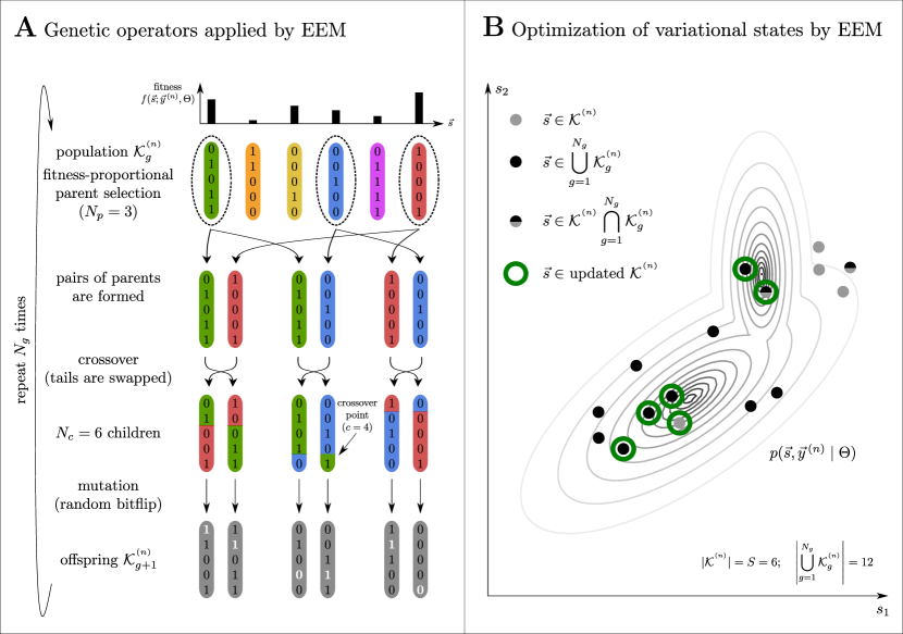
Figure 1: Illustration of the variational optimization using genetic operators.

The application of the genetic operators is iteratively repeated. The offspring $\mathcal{K}^{\phantom{1}{}^{(n)}}_{g+1}$ produced by the population $\mathcal{K}^{\phantom{1}{}^{(n)}}_{g}$ becomes the new population from which parents are selected (Figure 1). After $N_{g}$ iterations, we obtain a large number of new individuals (i.e., all the newly generated populations $\mathcal{K}^{\phantom{1}{}^{(n)}}_{g}$ with $g=1,\ldots,N_{g}$). The new populations of individuals can now be used to improve the original population $\mathcal{K}^{\phantom{1}{}^{(n)}}$ such that a higher value for the lower bound (4) is obtained. To find the best new population for a given $n$, we collect all generated populations (all $\mathcal{K}^{\phantom{1}{}^{(n)}}_{g}$ with $g=1,\ldots,N_{g}$) and unite them with $\mathcal{K}^{\phantom{1}{}^{(n)}}$. We then reduce this larger set back to the population size $S$, and we do so by only keeping those $S$ individuals with the highest joints $p(\vec{s},\vec{y}^{\,(n)}\mid\Theta)$. By only keeping the states/individuals with highest joints, the update procedure for $\mathcal{K}^{\phantom{1}{}^{(n)}}$ is guaranteed to monotonically increase the variational lower bound (4) since the variational bound is increased if criterion (5) is satisfied.

define selection, crossover and mutation operators;

set hyperparameters $S$, $N_{g}$, etc.;

initialize model parameters $\Theta$;

for each $n$: populate set $\mathcal{K}^{\phantom{1}{}^{(n)}}$ with $S$ latent states ($|\mathcal{K}^{\phantom{1}{}^{(n)}}|=S$);

repeat

       x=x 

      [-2mm] for $n=1,\ldots,N$ do

             set $\mathcal{K}^{\phantom{1}{}^{(n)}}_{0}=\mathcal{K}^{\phantom{1}{}^{(n)}}$;

            for $g=1,\ldots,N_{g}$ do

                   $\mathcal{K}^{\phantom{1}{}^{(n)}}_{g}=\text{mutation}\left(\text{crossover}\left(\text{selection}\left(\mathcal{K}^{\phantom{1}{}^{(n)}}_{g-1}\right)\right)\right)$;

                  $\mathcal{K}^{\phantom{1}{}^{(n)}}\,=\,\mathcal{K}^{\phantom{1}{}^{(n)}}\cup\mathcal{K}^{\phantom{1}{}^{(n)}}_{g}$;

            remove those $(|\mathcal{K}^{\phantom{1}{}^{(n)}}|-S)$ elements $\vec{s}$ in $\mathcal{K}^{\phantom{1}{}^{(n)}}$ with lowest $p(\vec{s},\vec{y}^{\,(n)}\,|\,\Theta)$;

      use M-steps with (3) to update $\Theta$;

until parameters $\Theta$ have sufficiently converged;

Algorithm 1 Evolutionary Expectation Maximization (EEM).

Algorithm 1 summarizes the complete variational algorithm; an illustration is provided in Figure 1. As the variational E-step is realized using an evolutionary algorithm, Algorithm 1 will from now on be referred to as Evolutionary Expectation Maximization (EEM). The EEM algorithm can be trivially parallelized over data-points. For later numerical experiments, we will use a parallelized implementation of EEM that can be executed on several hundreds of computing cores (for further technical details see Appendix E and also compare Salimans et al. 2017). For the numerical experiments, we will indicate which parent selection procedure (“fitparents” for fitness-proportional selection, “randparents” for random uniform selection) and which bitflip algorithm (“sparseflips” or “randflips”) are used in the variational loop. The term “cross” will be added to the name of the EA when crossover is employed.

2.2 Related Work on Applications of Evolutionary Approaches to Learning

Evolutionary algorithms (EAs) have repeatedly been applied to learning algorithms (e.g. Goldberg, 2006). In the context of reinforcement learning, for instance, evolution strategies have successfully been used as an optimization alternative to Q-learning and policy gradients (Salimans et al., 2017). EAs have also previously been applied to unsupervised learning based on generative models, also in conjunction with (or as substitute for) expectation maximization (EM). Myers et al. (1999) used EAs to learn the structue of Bayes Nets, for instance. Pernkopf and Bouchaffra (2005) have used EAs for clustering based on Gaussian mixture models (GMMs), where GMM parameters are updated relatively conventionally using EM. EAs are then used to select the best GMM models for the clustering problem (using a minimum description length criterion). Work by (Tohka et al., 2007) uses EAs for a more elaborate initialization of Finite Mixture Models, which is followed by EM. Work by Tian et al. (2011) goes further and combines EAs with a variational Bayes approach for GMMs. The algorithm they suggested is based on a fully Bayesian GMM approach with hyper-priors in the place of standard GMM parameters. The algorithm then first uses an EA to find good hyperparameters; given the hyperparameters the GMM is then trained using standard (but variational) EM iterations. The use of EAs by Pernkopf and Bouchaffra (2005) and Tian et al. (2011) is similar to their use for deep neural network (DNN) training. For DNNs, EAs are applied to optimize network hyperparameters in an outer loop (Stanley and Miikkulainen, 2002; Loshchilov and Hutter, 2016; Real et al., 2017; Suganuma et al., 2017; Oehmcke and Kramer, 2018, etc.) while DNN weight parameters are at the same time trained using standard back-propagation algorithms. Yet other approaches have applied EAs to directly optimize a clustering objective, using EAs to replace EM approaches for optimization (compare Hruschka et al., 2009). Similarly, in a non-probabilistic setting, EAs have been used to replace back-propagation for DNN training (see, e.g., Prellberg and Kramer, 2018, and references therein). Also in a non-probabilistic setting, for sparse coding with weights optimized based on a $l_{1}$-penalized reconstruction objective (e.g. Olshausen and Field, 1996), an EA tailored to this objective has been used to address maximum a-posteriori optimization (Ahmadi and Salari, 2016). In contrast to all such previous applications, the EEM approach (Algorithm 1) applies EAs as an integral part of variational EM, i.e., EAs address the key optimization problem of variational EM in the inner variational loop.

2.3 Data Estimator

As part of the numerical experiments, we will apply EEM to fit generative models to corrupted data which we will aim to restore; for instance we will apply EEM to denoise images corrupted by additive noise or to restore images with missing data (see Section 4). Here we illustrate how an estimator for such data reconstruction can be derived (details are given in Appendix C). Generally speaking, our aim is to compute estimates $\vec{y}^{\,\text{est}}$ based on observations $\vec{y}^{\,\text{obs}}$. If data points are corrupted by noise but not by missing values, we define the observations $\vec{y}^{\,\text{obs}}$ to be equal to the data points $\vec{y}\in\mathds{R}^{D}$ and we compute estimates $y_{d}^{\text{est}}$ for every $d=1,\dots,D$ with $D$ denoting the dimensionality of the data. In the presence of missing values, we define data points to consist of an observed part $\vec{y}^{\,\text{obs}}$ and a missing part $\vec{y}^{\,\text{miss}}=\vec{y}\,\backslash\vec{y}^{\,\text{obs}}$ and we aim to compute estimates $\vec{y}^{\,\text{est}}$ for the missing part. A data estimator can be derived based on the posterior predictive distribution $p(\vec{y}^{\,\text{est}}\mid\vec{y}^{\,\text{obs}})$. Here we will sketch how to derive an estimator for general models with binary latents and continuous observables (in Appendix C we provide a detailed derivation and show how to extend it to models with binary-continuous latents). The posterior predictive distribution for a model with binary latents and continuous observables is given by:

$$p(\vec{y}^{\,\text{est}}\mid\vec{y}^{\,\text{obs}},\Theta) =\sum_{\vec{s}}p(\vec{y}^{\,\text{est}}\,\mid\,\vec{s},\Theta)p(\vec{s}\,\mid\,\vec{y}^{\,\text{obs}},\Theta).$$ (8)

We choose to take expectations w.r.t. the posterior predictive distribution which leads to the following estimator:

$$\langle y_{d}^{\text{est}}\rangle_{p(\vec{y}^{\,\text{est}}\,\mid\,\vec{y}^{\,\text{obs}},\Theta)} =\left\langle\langle y_{d}^{\text{est}}\rangle_{p(y_{d}^{\text{est}}\,\mid\,\vec{s},\Theta)}\right\rangle_{p(\vec{s}\,\mid\,\vec{y}^{\,\text{obs}},\Theta)}.$$ (9)

The inner expectation in (9) can be identified with the mean of the distribution of the observables given the latents. This distribution is part of the definition of the generative model (compare Section 3.1). The outer expectation in $\eqref{eq:binlat_general_data_estimator_final}$ is taken w.r.t. the posterior distribution of the latents. Such expectation can efficiently be approximated using truncated expectations (3). Details and examples of data estimators for concrete models are given in Appendix C.

3 Application to Generative Models, Verification and Scalability

Considering Algorithm 1, observe that probabilistic inference for the algorithm is fully defined by the joint $p(\vec{s},\vec{y}^{\,(n)}\,|\,\Theta)$ of a given generative model and by a set of hyperparameters for the optimization procedure. No additional and model specific derivations are required for the variational E-step, which suggests Algorithm 1 for “black box” inference for models with binary latents. Using three different generative models, we here (A) verify this “black box” applicability, (B) numerically evaluate the algorithm’s ability to recover generating parameters, and (C) show scalability of the approach by applying it to large-scale generative models. To be able to study the properties of the novel variational optimization procedure, we consider generative models for which parameter update equations (M-steps) have been derived previously.

3.1 Used Generative Models

The generative models we use are noisy-OR Bayes Nets (binary latents and binary observables), Binary Sparse Coding (binary latents and continuous observables), and Spike-and-Slab Sparse Coding (continuous latents and continuous observables).

Noisy-OR Bayes Nets. A noisy-OR Bayes Net (e.g., Singliar and Hauskrecht, 2006; Jernite et al., 2013; Rotmensch et al., 2017) is a non-linear bipartite data model with all-to-all connectivity between the layer of hidden and observed variables (and no intra-layer connections). Latents and observables both take binary values, i.e. $\vec{s}\in\{0,1\}^{H}$ and $\vec{y}\in\{0,1\}^{D}$ with $H$ and $D$ denoting the dimensions of the latent and observed spaces. The model assumes a Bernoulli prior for the latents, and non-zero latents are then combined via the noisy-OR rule:

$$p\left(\vec{s}\mid\Theta\right)=\prod_{h=1}^{H}\mathcal{B}(s_{h};\pi_{h}),\;\;\;\;\;\;\;p\left(\vec{y}\mid\vec{s},\Theta\right)=\prod_{d=1}^{D}N_{d}(\vec{s}\,)^{y_{d}}(1-N_{d}(\vec{s}\,))^{1-y_{d}},\quad$$ (10)

where $\mathcal{B}(s_{h};\pi_{h})=\pi_{h}^{s_{h}}(1-\pi_{h})^{1-s_{h}}$ and where $N_{d}(\vec{s}\,)\vcentcolon=1-\prod_{h=1}^{H}(1-W_{dh}s_{h})$. In the context of the noisy-OR model $\Theta=\{\vec{\pi},W\}$, where $\vec{\pi}$ is the set of values $\pi_{h}\in[0,1]$ representing the prior activation probabilities for the hidden variables $s_{h}$ and $W$ is a $D{\times}H$ matrix of values $W_{dh}\in[0,1]$ representing the probability that an active latent variable $s_{h}$ activates the observable $y_{d}$. M-step update rules for the noisy-OR model can be derived by inserting (10) into the lower bound (1) and by then taking derivatives of the resulting expression w.r.t. all model parameters. The update rule for the $W$ parameter does not allow for a closed-form solution and a fixed-point equation is employed instead. The resulting M-step equations are shown in Appendix D.

Binary Sparse Coding. Binary Sparse Coding (BSC; Haft et al., 2004; Henniges et al., 2010) is an elementary sparse coding model for continuous data with binary latent and continuous observed variables. Similar to standard sparse coding (Olshausen and Field, 1997; Lee et al., 2007) BSC assumes that given the latents, the observables follow a Gaussian distribution. BSC and standard sparse coding differ from each other in their latent variables. In standard sparse coding, latents take continuous values and they are typically modeled e.g. with Laplace or Cauchy distributions. BSC uses binary latents $\vec{s}\in\{0,1\}^{H}$ which are assumed to follow a Bernoulli distribution $\mathcal{B}(s_{h};\pi)$ with the same activation probability $\pi$ for each hidden unit $s_{h}$. The combination of the latents is described by a linear superposition rule. Given the latents, the observables $\vec{y}\in\mathbbm{R}^{D}$ are independently and identically drawn from a Gaussian distribution:

$$p\left(\vec{s}\mid\Theta\right)=\prod_{h=1}^{H}\mathcal{B}(s_{h};\pi),\;\;\;\;\;\;\;p\left(\vec{y}\mid\vec{s},\Theta\right)=\prod_{d=1}^{D}\mathcal{N}(y_{d};\sum_{h=1}^{H}W_{dh}s_{h},\sigma^{2})$$ (11)

The parameters of the BSC model are $\Theta=(\pi,\sigma,W)$. $W$ is a $D\times H$ matrix whose columns contain the weights associated with each hidden unit; $\sigma$ determines the standard deviation of the Gaussian. The M-step equations for BSC can be derived analogously to the noisy-OR model by inserting (11) into (1) and by then optimizing the resulting expression w.r.t. each model parameter (compare, e.g., Henniges et al., 2010). As opposed to noisy-OR, each of the BSC update equations can be derived in closed-form. The explicit expressions are shown in Appendix D.

Spike-and-Slab Sparse Coding. As last example we consider a more expressive data model and use EEM to optimize the parameters of a spike-and-slab sparse coding (SSSC) model. SSSC extends the generative model of BSC in the sense that it uses a spike-and-slab instead of a Bernoulli prior distribution. The SSSC model has been used in a number of previous studies and in a number of variants (Titsias and Lázaro-Gredilla, 2011; Lücke and Sheikh, 2012; Goodfellow et al., 2012; Sheikh et al., 2014, and many more). It can be formulated using two sets of latents, $\vec{s}\in\{0,1\}^{H}$ and $\vec{z}\in\mathbbm{R}^{H}$, which are combined via pointwise multiplication s.t. $\left(\vec{s}\odot\vec{z}\,\right)_{h}=s_{h}z_{h}$. Here we take the continuous latents to be distributed according to a multivariate Gaussian with mean $\vec{\mu}$ and a full covariance matrix $\Psi$. The binary latents follow a Bernoulli distribution with individual activation probabilities $\pi_{h}$, $h=1,\dots,H$:

$$p\left(\vec{s}\mid\Theta\right)=\prod_{h=1}^{H}\mathcal{B}(s_{h};\pi_{h}),\;\;\;\;\;\;\;p\left(\vec{z}\mid\Theta\right)=\mathcal{N}(\vec{z};\vec{\mu},\Psi).\\$$ (12)

As in standard sparse coding, SSSC assumes components to combine linearly. The linear combination then determines the mean of a univariate Gaussian for the observables:

$$p\left(\vec{y}\mid\vec{s},\vec{z},\Theta\right)=\mathcal{N}(\vec{y};\,\sum_{h=1}^{H}\vec{W}_{h}s_{h}z_{h},\sigma^{2}\mathds{1})$$ (13)

where $W$ is a $D\times H$ matrix with columns $\vec{W}_{h}$ and where $\mathds{1}$ is the unit matrix. The M-step update rules of the SSSC model can be derived by taking derivatives of the free energy

$$\mathcal{F}(q,\Theta)=\sum_{n=1}^{N}\bigl{<}\log p(\vec{y}^{\,(n)},\vec{s},\vec{z}\mid\Theta)\bigr{>}_{q^{(n)}}\,+\,\sum_{n=1}^{N}H[q^{(n)}]$$ (14)

w.r.t. each of the model parameters $\Theta=(\vec{\pi},\sigma,W,\vec{\mu},\Psi)$. The term $\bigl{<}f(\vec{s},\vec{z})\bigr{>}_{q^{(n)}}$ in (14) denotes the expectation of $f(\vec{s},\vec{z})$ w.r.t. a variational distribution $q^{(n)}(\vec{s},\vec{z})$:

$$\bigl{<}f(\vec{s},\vec{z})\bigr{>}_{q^{(n)}}=\sum_{\vec{s}}\int q^{(n)}(\vec{s},\vec{z})f(\vec{s},\vec{z})\,\mathrm{d}\vec{z}.$$ (15)

The term $H[q^{(n)}]$ in (14) denotes the entropy $-\bigl{<}\log q^{(n)}(\vec{s},\vec{z})\bigr{>}_{q^{(n)}}$ of the variational distributions. For a detailed derivation of the SSSC M-step equations see Sheikh et al. (2014) and compare Goodfellow et al. (2012). For SSSC, all M-step updates (A) have closed-form solutions and (B) contain as arguments expectation values (15). Importantly for applying EEM, all these expectation values can be reformulated as expectations w.r.t. the posterior over the binary latent space. For more details see Appendix D and compare Sheikh et al. (2014). Based on the reformulations, the expectations w.r.t. the posterior over the binary latent space can be approximated using the truncated expectations (3). Since the joint $p(\vec{s},\vec{y}^{\,(n)}\mid\Theta)$ of the SSSC model is computationally tractable and given by

$$p\left(\vec{y}^{\,(n)},\vec{s}\mid\Theta\right)=\mathcal{B}(\vec{s};\vec{\pi})\,\,\mathcal{N}(\vec{y}^{\,(n)};\,\tilde{W}_{\vec{s}}\,\vec{\mu},C_{\vec{s}}),$$ (16)

with $C_{\vec{s}}=\sigma^{2}\mathds{1}+\tilde{W}_{\vec{s}}\,\Psi\,\tilde{W}_{\vec{s}}^{\mathrm{\,T}}$, $(\tilde{W}_{\vec{s}})_{dh}=W_{dh}s_{h}$ s.t. $W\left(\vec{s}\odot\vec{z}\,\right)=\tilde{W}_{\vec{s}}\,\vec{z}$, the variational lower bound (4) can be efficiently optimized using Algorithm 1. The EEM algorithm consequently provides a novel, evolutionary approach to efficiently optimize the parameters of the SSSC data model.

3.2 Verification: Recovery of Generating Parameters

First we verified EEM by training noisy-OR, BSC and SSSC models on artificial data for which the ground-truth generative parameters were known. We used the bars test as a standard setup for such purposes (Földiák, 1990; Hoyer, 2003; Lücke and Sahani, 2008). We started with a standard bars test using a weight matrix $W^{\mathrm{gen}}$ whose $H^{\mathrm{gen}}=2\sqrt{D}$ columns represented generative fields in the form of horizontal and vertical bars. We considered a dictionary of $H^{\mathrm{gen}}=10$ (Lücke and Sahani, 2008; Lücke and Eggert, 2010; Lücke et al., 2018; Sheikh and Lücke, 2016) components. For noisy-OR, we set the amplitudes of the bars and of the background to a value of 0.8 and 0.1, respectively; for BSC and SSSC the bar amplitudes were uniformly randomly set to 5 and -5 and the background was set to 0. For BSC and SSSC, we chose $(\sigma^{\mathrm{gen}})^{2}=1$ as ground-truth variance parameter; for SSSC we furthermore defined $\vec{\mu}^{\mathrm{gen}}=\vec{0}$ and $\Psi^{\mathrm{gen}}=\mathds{1}$.

For each model, 30 datasets of $N=5,000$ samples were generated. We used $\pi_{h}^{\mathrm{gen}}=\frac{2}{H^{\mathrm{gen}}}\,\forall\,h=1,\dots,H^{\mathrm{gen}}$ (see Figure 2 for a few examples). We then applied EEM to train noisy-OR, BSC and SSSC models with $H=H^{\mathrm{gen}}=10$ components (EEM hyperparameters are listed in Table 3 in Appendix E). For noisy-OR, priors $\pi_{h}$ were initialized to an arbitrary sparse value (typically $\frac{1}{H}$) while the initial weights $W^{\mathrm{init}}$ were sampled from the standard uniform distribution. The $\mathcal{K}^{\phantom{1}{}^{(n)}}$ sets were initialized by sampling bits from a Bernoulli distribution that encouraged sparsity. In our experiments, the mean of the distribution was set to $\frac{1}{H}$. For BSC, the initial value of the prior was defined $\pi^{\mathrm{init}}=\frac{1}{H}$; the value of $(\sigma^{\mathrm{init}})^{2}$ was set to the variance of the data points averaged over the observed dimensions. The columns of the $W^{\mathrm{init}}$ matrix were initialized with the mean of the data points to which some Gaussian noise with a standard deviation of $0.25\,\sigma^{\mathrm{init}}$ was added. The initial values of the $\mathcal{K}^{\phantom{1}{}^{(n)}}$ sets were drawn from a Bernoulli distribution with $p(s_{h}=1)=\frac{1}{H}$. To initialize the SSSC model, we uniformly randomly drew $\vec{\pi}^{\mathrm{init}}$ and $\vec{\mu}^{\mathrm{init}}$ from the interval $[0.1,0.5]$ and $[1,5]$, respectively (compare Sheikh et al., 2014) and set $\Psi^{\mathrm{init}}$ to the unit matrix. For SSSC, we proceeded as we had done for the BSC model to initialize the dictionary $W$, the variance parameter $\sigma^{2}$ and the sets $\mathcal{K}^{\phantom{1}{}^{(n)}}$. The evolution of the model parameters during learning is illustrated in Figure 2 for an exemplary run of the “fitparents-randflip” EA (illustrations of the parameters $\sigma$ of the BSC model and $\Psi$, $\vec{\mu}$ and $\sigma$ of the SSSC model are depicted in Figure 8 in Appendix F).

Figure 2: Training noisy-OR (NOR), BSC and SSSC models on artificial data using EEM.

Figure 2 illustrates that the ground-truth generative parameters can accurately be recovered for each model using EEM. The weights, latent means and latent covariances of the SSSC model are recovered in scaled versions w.r.t. the ground-truth values. This effect can be considered as a consequence of the spike-and-slab prior which allows for multiple equivalent solutions for the amplitudes of $W$ and $\vec{z}$ given a data point. We further used the setup with artificial data and known ground-truth generative parameters to explore EAs with different types of combinations of genetic operators. Different combinations of genetic operators resulted in different degrees of ability to recover the ground-truth parameters. For instance, for noisy-OR trained with EEM, the combination of random uniform parent selection, single-point crossover and sparsity-driven bitflip (“randparents-cross-sparseflips”) resulted in the best behavior for bars test data (also compare Guiraud et al., 2018). For BSC and SSSC trained with EEM, the best operator combinations were “fitparents-cross-sparseflips” and “fitparents-randflips”, respectively (compare Figure 9 in Appendix F). In general, the best combination of operators will depend on the data model and the data set used.

3.3 Scalability to Large Generative Models

Having verified the ability of EEM to recover ground-truth generating parameters for the three generative models of Section 3.1, we continued with investigating how well the evolutionary approximation was able to optimized large-scale models. Scalability is a property of crucial importance for any approximation method, and large-scale applicability is essential to accomplish many important data processing tasks based on generative models. To investigate scalability, we used natural image patches which are known to be richly structured and which require large models to appropriately model their distribution. We used image patches extracted from a standard image database (van Hateren and van der Schaaf, 1998). We trained the noisy-OR, BSC and SSSC data models using the “fitparents-cross-sparseflips” variant of EEM as we observed this operator combination to perform well across all models for this data.

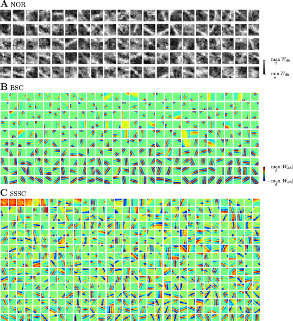
Figure 10: Dictionaries learned from natural image patches using noisy-OR, BSC and SSSC models (see Section 3.3). For noisy-OR, we considered raw image patches and trained a model with $H=100$ components. For BSC and SSSC, image patches were preprocessed using a whitening procedure. For BSC and SSSC, $H=300$ and $H=512$ generative fields were learned, respectively. In B and C, the fields are ordered according to their activation, starting with the fields corresponding to the most active hidden units.

For noisy-OR, we considered raw images patches, i.e., images which were not mean-free or whitened and reflected light intensities relatively directly. We used image patches that were generated by extracting random $10\times 10$ subsections of a single $255\times 255$ image of overlapping grass wires (part of image 2338 of the database). We clamped the brightest 1 % pixels from the dataset, and scaled each patch to have gray-scale values in the range $[0,1]$. From these patches, we then created $N=30,000$ data points $\vec{y}^{\,(n)}$ with binary entries by repeatedly choosing a random gray-scale image and sampling binary pixels from a Bernoulli distribution with parameter equal to the pixel values of the patches with $[0,1]$ gray-scale. Because of mutually occluding grass wires in the original image, the generating components of the binary data could be expected to follow a non-linear superimposition, which motivated the application of a non-linear generative model such as noisy-OR. For the data with $D=10\times 10=100$ observables, we applied a noisy-OR model with $H=100$ latents (EEM hyperparameters are listed in Table 3 in Appendix E). During training, we clamped the priors $\pi_{h}$ to a minimum value of $1/H$ to encourage the model to make use of all generative fields. Figure 3 (top) shows a random selection of 50 generative fields learned by the noisy-OR model (the full dictionary is displayed in Figure 10 in Appendix F). Model parameters initialization followed the same procedure as for the bars tests. EEM parameters are listed in Table 3 in Appendix E. As can be observed, EEM is efficient for large-scale noisy-OR on real data. Many of the generative fields of Figure 3 (top) resemble curved edges, which is in line with expectations and with results, e.g., as obtained by Lücke and Sahani (2008) with another non-linear generative model.

For the BSC generative model, we are not restricted to positive data. Therefore, we can use a whitening procedure as is customary for sparse coding approaches (Olshausen and Field, 1997). We employed $N=100,000$ image patches of size $D=16\times 16=256$ which were randomly picked from the van Hateren dataset. The highest 2 % of the pixel values were clamped to compensate for light reflections, and patches without significant structure were removed to prevent amplifications of very small intensity differences. The whitening procedure we subsequently applied is based on ZCA whitening (Bell and Sejnowski, 1997) retaining 95 % of the variance (compare Exarchakis and Lücke, 2017). We then applied EEM to fit a BSC model with $H=300$ components to the data (EEM hyperparameters are listed in Table 3 in Appendix E). To initialize the model and the variational parameters, we proceeded as we had done for the bars test (Section 3.2). Figure 3 (middle) depicts some of the generative fields learned by the BSC model. The fields correspond to the 60 hidden units with highest prior activation probability (for the full dictionary see Figure 10 in Appendix F). The obtained generative fields primarily take the form of the well-known Gabor functions with different locations, orientations, phase, and spatial frequencies.

We collected another $N=100,000$ image patches of size $D=12\times 12=144$ from the van Hateren dataset to fit a SSSC model with $H=512$ components (EEM hyperparameters listed in Table 3 in Appendix E). We applied the same preprocessing as for the BSC model and initialized the model and the variational parameters similarly to the bars test. Figure 3 (bottom) shows a random selection of 60 out of the 512 generative fields learned by the SSSC model (the full dictionary is displayed in Figure 10 in Appendix F). The experiment shows that EEM can be applied to train complex generative models on large-scale realistic data sets; the structures of the learned generative fields (a variety of Gabor-like and a few globular fields) are in line with observations made in previous studies which applied SSSC models to whitened image patches (see, e.g., Sheikh and Lücke, 2016).

Figure 3: Dictionary elements learned by noisy-OR (top), BSC (middle) and SSSC (bottom) models on natural image patches. The models were trained on separate datasets that had been obtained using different preprocessing schemes (see text). For noisy-OR, a random selection of 50 out of 100 fields is displayed; for BSC the fields corresponding to the 60 out of 300 most active hidden units are shown; for SSSC a random selection of 60 out of 512 fields is displayed. The full dictionaries learned by the individual models are depicted in Figure 10 in Appendix F.

4 Performance Comparison on Denoising and Inpainting Benchmarks

So far, we have verified that EEM can be applied to the training of elementary generative models such as noisy-OR Bayes Nets and Binary Sparse Coding (BSC) but also to the more expressive model of spike-and-slab sparse coding (SSSC) which features a more flexible prior than BSC or standard sparse coding. To perform variational optimization for these models, no additional analytical steps were required and standard settings of optimization parameters were observed to work well. However, an important question is how well EEM is able to optimize model parameters compared to other methods. And more generally, how well do generative model algorithms perform in benchmarks if their parameters are optimized by EEM? Here we will address these questions using two standard and popular benchmarks: image denoising and image inpainting. These two benchmarks offer themselves for performance evaluation, as benchmark data is available for a large range of different algorithms (including algorithms based on generative models among many others). The data for standard denoising and inpainting benchmarks is continuous. We will consequently focus on the BSC and SSSC generative models. In the following, we will refer to EEM applied to BSC as Evolutionary Binary Sparse Coding (EBSC) and to EEM applied to SSSC as Evolutionary Spike-and-Slab Sparse Coding (ES3C). As genetic operator combination for the EA we will use “fitparents-randflips” for all the following experiments. The main reason to prefer this combination over combinations that also use cross-over is computational efficiency (which is a major limiting factor for the following experiments).

4.1 Algorithm Types and Comparison Categories

We will use standard benchmarks to compare EBSC and ES3C w.r.t. (A) algorithms based on generative models equal or similar to the ones used in this work, (B) other probabilistic methods including mixture models and Markov random fields approaches, (C) non-local image specific methods and (D) deep neural networks. Table 1 gives an overview of the methods we compare to, sorted by algorithm type. To the knowledge of the authors, the listed papers represent the best performing approaches while we additionally included standard baselines such as BM3D, EPLL or MLP (see Table 1 for references).

The algorithms listed in Table 1 have different requirements that have to be fulfilled for them to be applicable. To facilitate comparison, we have grouped the benchmarked algorithms into the different categories of prior knowledge they require (see Table 2 and Appendix G for a related discussion). As can be observed, some algorithms (e.g., KSVD or BM3D) require the noise level to be known a-priori, for instance. Others do require (often large amounts of) clean images for training, which typically applies for feed-forward deep neural networks (DNNs). If an algorithm is able to learn without information other than the corrupted image itself, it is commonly referred to as a “zero-shot” learning algorithm (compare, e.g., Shocher et al., 2018; Imamura et al., 2019). Algorithms of the “zero-shot” category we compare to are, e.g., MTMKL, BPFA and DIP. The EEM-based algorithms EBSC and ES3C also fall into the “zero-shot” category. In Table 2, we have labeled the categories DE1-DE6 for denoising and IN1-IN6 for inpainting. DE2 could also be referred to as “zero-shot + noise level” as the algorithms of that category also do not need additional images.

Acronym	Algorithm Name / Type	Reference
Sparse Coding / Dictionary Learning
MTMKL	Spike-and-Slab Multi-Task and Multiple Kernel Learning	Titsias and Lázaro-Gredilla 2011
BPFA	Beta Process Factor Analysis	Zhou et al. 2012
GSC	Gaussian Sparse Coding	Sheikh et al. 2014
KSVD	Sparse and Redundant Representations Over Trained Dictionaries	Elad and Aharon 2006
cKSVD	Sparse Representation for Color Image Restoration	Mairal et al. 2008
LSSC	Learned Simultaneous Sparse Coding	Mairal et al. 2009
BKSVD	Bayesian K-SVD	Serra et al. 2017
Other Probabilistic Methods (GMMs, MRFs)
EPLL	Expected Patch Log Likelihood	Zoran and Weiss 2011
PLE	Piecewise Linear Estimators	Yu et al. 2012
FoE	Fields of Experts	Roth and Black 2009
MRF	Markov Random Fields	Schmidt et al. 2010
NLRMRF	Non-Local Range Markov Random Field	Sun and Tappen 2011
Non-Local Image Processing Methods
BM3D	Block-Matching and 3D Filtering	Dabov et al. 2007
NL	Patch-based Non-Local Image Interpolation	Li 2008
WNNM	Weighted Nuclear Norm Minimization	Gu et al. 2014
Deep Neural Networks
MLP	Multi Layer Perceptron	Burger et al. 2012
DnCNN-B	Denoising Convolutional Neural Network	Zhang et al. 2017
TNRD	Trainable Nonlinear Reaction Diffusion	Chen and Pock 2017
MemNet	Deep Persistent Memory Network	Tai et al. 2017
IRCNN	Image Restoration Convolutional Neural Network	Chaudhury and Roy 2017
FFDNet	Fast and Flexible Denoising Convolutional Neural Network	Zhang et al. 2018
DIP	Deep Image Prior	Ulyanov et al. 2018
DPDNN	Denoising Prior Driven Deep Neural Network	Dong et al. 2019
BDGAN	Image Blind Denoising Using Generative Adversarial Networks	Zhu et al. 2019
BRDNet	Batch-Renormalization Denoising Network	Tian et al. 2020

Table 1: Algorithms used for comparsion on denoising and/or inpainting benchmarks. The algorithms have been grouped into four types of approaches. The table includes the best performing algorithms and standard baselines.

A Denoising	B Inpainting
Further a-priori knowledge required None Noise Level Test-Train Match Clean training data required No DE1 DE2 DE3 MTMKL BPFA GSC BKSVD EBSC ES3C KSVD LSSC BM3D WNNM n/a Yes DE4 DE5 DE6 n/a EPLL MLP DnCNN-B TNRD MemNet FFDNet DPDNN BDGAN BRDNet	Further a-priori knowledge required None Noise Level Test-Train Match Clean training data required No IN1 IN2 IN3 MTMKL BPFA BKSVD DIP ES3C NL PLE n/a Yes IN4 IN5 IN6 FoE MRF cKSVD NLRMRF IRCNN

Table 2: Algorithms for denoising and inpainting require different degrees and types of prior knowledge. In A the algorithms listed in the column “Noise Level” require the ground-truth noise level of the test data as input parameter. The denoising approaches listed in the column “Test-Train Match” are optimized either for one single or for several particular noise levels. In B the column “Test-Train Match” lists inpainting algorithms that are optimized for a particular percentage of missing pixels (e.g. for images with 80% randomly missing values) or for a particular missing value pattern. These algorithms (category IN6) can be applied without providing a mask that indicates the pixels that are to be filled (see Appendix G for details).

4.2 Image Denoising

To apply EBSC and ES3C for image denoising, we first preprocessed the noisy images that we aimed to restore by segmenting the images into smaller patches: given an image of size $\cal{H}\times\cal{W}$ and using a patch size of $D=P_{x}\times P_{y}$ we cut all possible $N=(\cal{W}-\cal{P}_{\text{x}}+\text{1})\times(\cal{H}-\cal{P}_{\text{y}}+\text{1})$ patches by moving a sliding window on the noisy image. Patches were collected individually for each image and corresponded to the datasets $\mathcal{Y}$ which EBSC or ES3C were trained on. In other words, EBSC and ES3C leveraged nothing but the information of the noisy image itself (no training on other images, no training on clean images, noise unknown a-priori). After model parameters had been inferred using EBSC and ES3C, we took expectations w.r.t. the posterior predictive distribution of the model in order to estimate the non-noisy image pixels. For each noisy patch, we estimated all its non-noisy pixel values, and as commonly done we repeatedly estimated the same pixel value based on different (mutually overlapping) patches that shared the same pixel. The different estimates for the same pixel were then gathered to determine the non-noisy value using a weighted average (for details see Section 2.3 and Appendix C; also see, e.g., Burger et al. 2012). Finally, we were interested in how well EBSC and ES3C could denoise a given image in terms of the standard peak-signal-to-noise ratio (PSNR) evaluation measure.

4.2.1 Relation between PSNR measure and variational lower bound

We first investigated whether the value of the learning objective (the variational lower bound) of EBSC and ES3C was instructive about the denoising performance of the algorithms in terms of PSNR. While the PSNR measure requires access to the clean target image, the learning objective can be evaluated without such ground-truth knowledge. If learning objective and PSNR measure were reasonably well correlated, one could execute the algorithms several times on a given image and determine the best run based on the highest value of the learning objective without requiring access to the clean image. For the experiment, we used the standard “House” image degraded by additive white Gaussian (AWG) noise with a standard deviation of $\sigma=50$ (the clean and noisy images are depicted in Figure 5). We applied ES3C for denoising using patches of size $D=8\times 8$ and a dictionary with $H=256$ elements (EEM hyperparameters listed in Table 3 in Appendix E). At several iterations during execution of the algorithm, we measured the value of the learning objective and the PSNR of the reconstructed image. The experiment was repeated five times, each time using the same noisy image but a different initialization of the algorithm. Figure 4 illustrates the result of this experiment.

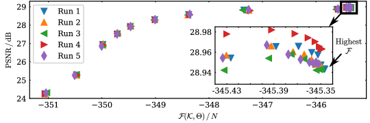
Figure 4: Variational bound and PSNR value pairs obtained from applying ES3C to the noisy “House” image (AWG noise with $\sigma=50$). 2,000 EEM iterations were performed and PSNR values were measured at iterations 1, 2, 5, 10, 20, 50, 100, 200, 400, 600, 800, 1000, 1200, 1400, 1600, 1800, 2000. The experiment was repeated five times using the same noise realization in each run. The PSNR values at the last iteration were 28.94, 28.95, 28.94, 28.96, 28.95 (avg. rounded $28.95\pm 0.01$; all values in dB).

As can be observed, PSNR values increase with increasing value of the objective $\mathcal{F}(\mathcal{K},\Theta)\,/\,N$ during learning. The truncated distributions which give rise to the lower bound are consequently well suited. Only at the end of learning, PSNR values slightly decrease while the lower bound still increases (inset figure). The final PSNR decreases are likely due to the PSNR measure being not perfectly correlated with the data likelihood. However, decreases of the likelihood while the lower bound still increases cannot be excluded. While final decreases of PSNR are small (see scale of inset figure of Figure 4), their consequence is that the run with the highest final value for the variational bound is not necessarily the run with the highest PSNR. For Figure 4, for instance, Run 1 has the highest final variational bound but Run 4 the highest final PSNR.

4.2.2 Comparison of Generative Models and Approximate Inference

Before comparing EBSC and ES3C with a broad range of different denoising algorithms (further below), we first focused on approaches that are all based on essentially the same data model. Differences in measured performance can than be attributed more directly to differences in the method used for parameter optimization. Concretely, we here first consider algorithms that are all based on a spike-and-slab sparse coding (SSSC) model. Namely, we compare the following algorithms:

• the ES3C algorithm which is trained using variational optimization of truncated posteriors (EEM),

• the MTMKL algorithm (Titsias and Lázaro-Gredilla, 2011) which uses a factored variation approach (i.e., mean field) for parameter optimization (also compare Goodfellow et al., 2012),

• the BPFA algorithm (Zhou et al., 2012) which uses sampling for parameter optimization,

• the GSC algorithm (Sheikh et al., 2014) which uses truncated posteriors constructed using preselection (i.e., no variational loop).

Furthermore, we included EBSC into the comparison, as the BSC data model (Henniges et al., 2010) is a boundary case of the SSSC model. For best comparability, we investigated the denoising performance of the algorithms under controlled conditions: We considered a fixed task (the “House” benchmark with $\sigma=50$ AWG noise), and we compared algorithms for three different configurations of $D$ and $H$ (see Figure 5 B). PSNR values for BPFA, MTMKL and GSC are taken from the corresponding original publications. The publication for GSC only reports values for $D=8\times{}8$ and $H=64$ as well as for $D=8\times{}8$ and $H=256$; MTMKL only for the former and BPFA only for the latter setting. We additionally cite the performance of MTMKL for $D=8\times{}8$ and $H=256$ as reported by Sheikh et al. (2014). PSNR values for the algorithms EBSC and ES3C were obtained as described above (Section 4.2) using the same hyperparameters for both approaches (see Table 3 in Appendix E). The PSNR values for EBSC and ES3C are averages across three runs each (standard deviations were smaller or equal 0.13 dB PSNR).

Considering Figure 5 B, BPFA and MTMKL (which both represented the state-of-the-art at the time of their publication) perform well but in comparison ES3C shows significant further improvements. As the major difference between the considered approaches is the parameter optimization approach rather than the generative model, the performance increases of ES3C compared to the other algorithms can be attributed to the used EEM optimization. An important factor of the performance increases for ES3C is presumably its ability to leverage the available generative fields more effectively. Titsias and Lázaro-Gredilla (2011) report for MTMKL, for instance, that larger dictionaries ($H>64$) do not result in performance increases; similarly Zhou et al. (2012) report that BPFA models with 256 and 512 dictionary elements yield similar performance. GSC has been shown to make better use of larger dictionaries than MTMKL (Sheikh et al., 2014). Performance of GSC is, however, significantly lower than ES3C for all investigated dictionary sizes, which provides strong evidence for the advantage of the fully variational optimization used by EEM. The EEM optimization also results in a notably strong performance of EBSC compared to previous approaches: it outperforms MTMKL (as well as GSC for $H=64$). The strong performance may be unexpected as the underlying BSC model is less expressive than the SSSC data model. The performance gains using EEM thus outweigh the potentially better data model in this case. However, ES3C performs (given the same set of hyperparameters) much stronger than EBSC in all settings, and can make much more use of larger dictionaries and larger patches.

4.2.3 General comparison of denoising approaches

After having compared a selected set of algorithms under controlled conditions, we investigated denoising performance much more generally. We compared the best performing algorithms on standard denoising benchmarks irrespective of the general approach they follow, allowing for different task categories they require, and allowing for any type of hyperparameters they use. The methods we have used for comparison are listed in Table 2 A, where the algorithms are grouped according to the prior information they assume (compare Section 4.1 and Appendix G).

A limitation of most of the investigated algorithms is the computational resources they require. For EBSC and ES3C, model size (i.e., patch and dictionary sizes) are limited by available computational resources and so is the number of variational states $S$ (Section 2.1) used to approximate posteriors. For ES3C, a good trade-off between performance vs. computational demand was observed for instance for $D=12\times 12$ and $H=512$ with $S=60$ for the experiment of Figure 5 D; for EBSC a good trade-off between performance and computational demand was observed for $D=8\times 8$ and $H=256$ with $S=200$. We thus have used more variational states $S$ for EBSC than for ES3C. Technical details including EEM hyperparameters are provided in Appendix E.

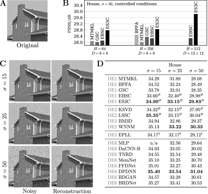
Figure 5: Denoising results for the “House” image (clean original depicted in A). B Performance comparison for AWG noise with $\sigma=50$ under controlled conditions (see text for further details). D Performance comparison w.r.t. to state-of-the-art denoising approaches and standard baselines using different optimized hyperparameters (see text for further details). Grouping and labeling according to Table 2; in each group the highest PSNR value is marked bold. Numbers marked with ^∅correspond to averages over multiple independent realizations of the experiment using different realizations of the noise (see text for further details). For EPLL, model selection was performed based on the learning objective of the algorithm (^†markers; personal communication with D. Zoran). Panel C illustrates the reconstructed images obtained with ES3C in the run with the highest PSNR value.

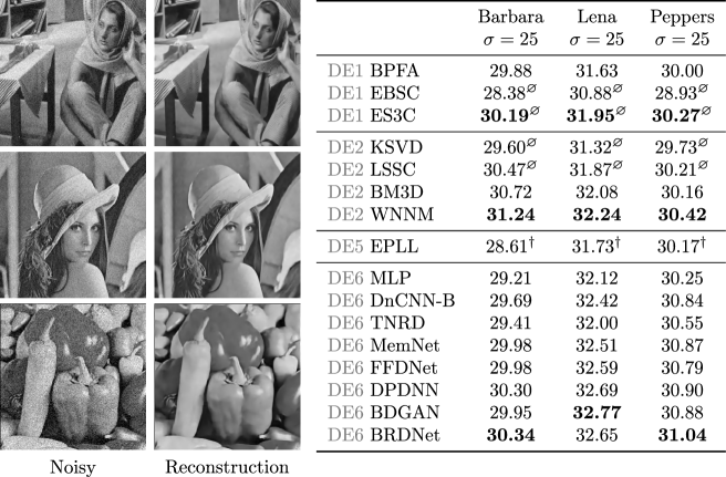
Figure 6: Denoising results for “Barbara”, “Lena” and “Peppers”. The table shows a performance comparison w.r.t. to state-of-the-art denoising approaches and standard baselines using different optimized hyperparameters (see text for further details). Grouping and labeling according to Table 2; in each group the highest PSNR value is marked bold. Numbers marked with ^∅correspond to averages over multiple independent realizations of the experiment using different realizations of the noise (see text for further details). For EPLL, model selection was performed based on the learning objective of the algorithm (^†markers; personal communication with D. Zoran). On the left we illustrate the reconstructed images obtained with ES3C in the run with the highest PSNR value.

Figures 5 D and 6 list denoising performances obtained with algorithms from the different categories of Table 2. The listed PSNR values are taken from the respective original publications with the following exceptions: For WNNM, EPLL and MLP, values are taken from Zhang et al. (2017) and for TNRD and MemNet values equal the ones in Dong et al. (2019). PSNR values reported in the original papers are often single PSNR values which may correspond to a single run of the investigated algorithm or to the best observed PSNR value. For deterministic methods with essentially no PSNR variations for a fixed input, it might seem natural to report a single PSNR value. For stochastic methods, reporting the best observed value is instructive about how well a given method can in principle perform. In practice, however, the run with highest PSNR value is less relevant than the average PSNR as selecting the run with best PSNR usually requires ground-truth (compare discussion in Appendix G). For KSVD and LSSC as well as for EBSC and ES3C, the PSNR values listed in Figures 5 D and 6 correspond to averages. For the two former approaches, averages were obtained from five runs of the algorithms with different noise realizations (standard deviations were reported to be negligibly small; see Elad and Aharon 2006, Mairal et al. 2009). For EBSC and ES3C, we performed three runs of the algorithms with different noise realizations (observed standard deviations of the resulting PSNRs were not larger than 0.06 dB; compare Table 4 in Appendix F).

Considering Figures 5 D and 6, it can be observed that the performance tends to increase the more a-priori information is used by an algorithm (as can be expected). Feed-forward DNNs report overall the best PSNR values but also use the most a-priori information (see category DE6, Table 2). In the “zero-shot” category with no a-priori information (DE1), ES3C shows the best performance (Figure 5 D). ES3C significantly increases the state-of-the-art PSNR values across all investigated settings. ES3C is still competitive if compared to algorithms in categories DE2 and DE5 which use more a-priori information but it is outperformed by some of these methods especially at lower noise levels (Figures 5 D and 6). Notably, differences in performance between the categories get smaller for larger and more complex images (Figure 6). For the image “Barbara”, for instance, ES3C outperforms all DNNs except of DPDNN and BRDNet which are slightly better while the best result is obtained for the image specific non-local method WNNM.

PSNR values achieved by the previous methods of BPFA or MTMKL have notably proven to be difficult to further improve. Only systems using more a-priori information (such as WNNM in category DE2 or DNNs in category DE6) have more recently reported higher PSNR values (also see discussion of difficult to improve BM3D values by Gu et al., 2014). In category DE1, the only more recent competitive approach is a Bayesian version of K-SVD (BKSVD; Serra et al., 2017). By extending K-SVD using Bayesian methodology, the data noise can be estimated from data. The BKSVD approach can thus be applied without a-priori information on the noise level, which makes it applicable in the “zero-shot” category (see Serra et al., 2017, for a discussion). PSNR values for BKSVD reported by Serra et al. 2017 are computed on downscaled images, and are therefore not directly comparable to those of Figures 5 D and 6. However, comparisons of BKSVD with MTMKL, K-SVD and BPFA reported by Serra et al. (2017) show that BKSVD performs competitive especially for lower noise levels. For higher noise levels, though, (e.g. $\sigma=25$ for ‘Lena’ and ‘Peppers’) BPFA results in higher PSNR values (and in similar PSNRs for ‘Barbara’). As ES3C outperforms BPFA for $\sigma=25$ on ‘Barbara’, ‘Lena’ and ‘Peppers’ on the full resolution images, BKSVD also does not seem to establish a new state-of-the-art in the DE1 category. We can, therefore, conclude that ES3C establishes a novel state-of-the-art in the “zero-shot” category since a relatively long time.

4.3 Image Inpainting

The final benchmark we used is image inpainting, i.e., the reconstruction of missing values in images. A standard setting for this task is the restoration of images that have been artificially degraded by uniformly randomly deleting pixels. We here considered the standard test images “Barbara”, “Cameraman”, “Lena”, “House” and “Castle” as examples for gray-scale and RGB images. For denoising, ES3C consistently performed better than EBSC, and the same we observed for inpainting. The performance difference between ES3C and EBSC on inpainting was, however, larger (sometimes several dB). We therefore focus on ES3C for comparison as EBSC is not competitive to the best performing methods we compare to.

For inpainting with ES3C, we employed the same partitioning and averaging scheme as described in Section 4.2. For the RGB image, ES3C was applied jointly to all color channels, as this had been reported to be more beneficial than training individual models on different color layers (Mairal et al., 2008). We trained the model and restored missing values exclusively based on the incomplete data which we aimed to restore (following, e.g., Fadili and Starck 2005; Little and Rubin 1987); uncorrupted pixels were not modified. Details about the missing value estimator applied by ES3C are provided in Section 2.3 and in Appendix C. For inpainting, we used a SSSC model with fixed $\vec{\mu}=\vec{1}$ and $\Psi=\mathds{1}$ as these parameters were observed to grow exponentially during learning which led to numerical instabilities of the training process. For each test scenario, we performed three runs of ES3C and used a different realization of missing values in each run (EEM hyperparameters are listed in Table 3 in Appendix E). Compared to the denoising experiments (Section 4.2.3), we observed for inpainting slightly larger variations of the resulting PSNR values (standard deviations were smaller or equal 0.18 dB; results of individual runs listed in Table 4 in Appendix F).

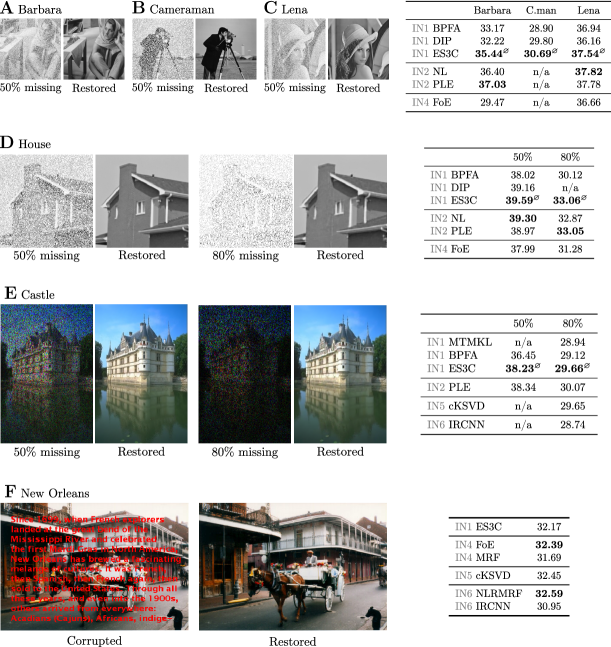
Figure 7: Inpainting results for “Barbara”, “Cameraman”, “Lena”, “House”, “Castle” and “New Orleans”. For the performance comparison, different approaches are grouped and labeled according to Table 2. In each group, the highest PSNR value is marked bold. Numbers marked with ^∅in A to E correspond to averages over multiple independent runs of the experiment using different realizations of missing values (see text for details; the performance of ES3C in the individual runs is reported in Table 4 in Appendix F). On the left we illustrate the reconstructed images obtained with ES3C in the run with the highest PSNR value.

The inpainting results for “Barbara”, “Cameraman”, “Lena” (each 50% missing values) and “House” and “Castle” (each 50% and 80% missing values) are depicted in Figure 7 A-E. The reference PSNR values are taken from the original publications except for NL and FoE for which we cite the numbers as reported by Yu et al. (2012). In general, inpainting is a less wide-spread benchmark than denoising presumably because additional estimation routines have to be developed and missing values pose, more generally, a considerable challenge to many approaches. Considering Figure 7 A-E, first observe that performance differences between categories are larger than for denoising. Compared to the best performing approaches in the literature, ES3C shows to be competitive in many settings. On the “Castle” benchmark, ES3C performs better than all other approaches in the literature except of PLE which uses the noise level as a-priori information. For the “House” benchmark, ES3C establishes a novel state-of-the-art in general: it performs better than all other algorithms for $50\%$ lost pixels and equal to PLE for $80\%$ lost pixels (i.e., within PSNR standard deviation of ES3C). This novel state-of-the-art is notably reached without requiring clean training data or a-priori knowledge about noise level or sparsity (ES3C requires to know which pixels are missing; compare Table 2 and Appendix G).

Finally, we also report inpainting performance on the well-known “New Orleans” inpainting benchmark (Figure 7 F left-hand-side). The benchmark serves as an inpainting example where pixels are lost non-randomly. For the benchmark, the original image is artificially corrupted by adding overlaid text, which is then removed by applying inpainting. Compared to inpainting with randomly missing values (e.g., the benchmarks in Figure 7 A-E), the “New Orleans” image contains relatively large contiguous regions of missing values. For our measurements, we used a publicly available dataset. The result of the experiment is illustrated in Figure 7 F. Reference PSNR values are taken from respective original publications with exceptions of FoE and MRF for which we use values reported by Sun and Tappen (2011). Due to extensive runtimes, we report the result of a single run of ES3C for this benchmark (see Appendix E for further details; EEM hyperparameters listed in Table 3). As can be observed, ES3C also performs well on this task. We observed higher PSNR values for ES3C than for MRF and IRCNN. Values for FoE and cKSVD are higher but also more a-priori information is used. Especially FoE is less sensitive to larger areas of lost pixels than ES3C (compare the lower performance of FoE in Figure 7 A-D); presumably FoE can make better use of larger contexts. The state-of-the-art on this benchmark is established by NLRMRF.

5 Discussion

Efficient approximate inference is of crucial importance for the training of expressive generative models. Consequently, there exist a range of different methods with different assumptions and different features. As most generative models can only be trained using approximations and usually many locally optimal solutions exist, the question of how well a generative model can potentially perform on a given task is difficult to answer. Sophisticated, mathematically grounded approaches such as sampling or variational optimization have been developed in order to derive sufficiently precise and efficient learning algorithms. As a contribution of this work, we have proposed a general purpose variational optimization that directly and intimately combines evolutionary algorithms (EAs) and EM. Considering Algorithm 1, EAs are an integral part of variational EM where they address the key optimization problem (the variational loop) arising in the training of directed generative models. The EEM algorithm is defined by a set of optimization hyperparameters for the EA. Given the hyperparameters, EEM is applicable to a given generative model solely by using the model’s joint probability $p(\vec{s},\vec{y}\,|\,\Theta)$. No analytical derivations are required to realize variational optimization.

Relation to other approximate inference approaches. To show large-scale applicability of EEM, we considered high-dimensional image data and generative models with large (combinatorial) state spaces. Aside from the elementary generative models of noisy-OR Bayes Nets (Singliar and Hauskrecht, 2006; Jernite et al., 2013; Rotmensch et al., 2017) and binary sparse coding (Haft et al., 2004; Henniges et al., 2010), we used spike-and-slab sparse coding (SSSC) as a more expressive example. The SSSC data model has been of considerable interest due to its strong performance for a range of tasks (Zhou et al., 2009, 2012; Titsias and Lázaro-Gredilla, 2011; Goodfellow et al., 2012; Sheikh et al., 2014). However, its properties require sophisticated probabilistic approximation methods for parameter optimization. Essentially three types of approximations have previously been applied to train the model: mean field (Titsias and Lázaro-Gredilla, 2011; Goodfellow et al., 2012), truncated posterior approximations (Sheikh et al., 2014), and MCMC sampling (Zhou et al., 2009, 2012; Mohamed et al., 2012). The EEM method shares features with all three previous approaches: like work by Sheikh et al. (2014), EEM uses truncated posterior distributions to approximate full posteriors, which contrasts with factored posterior approximations (i.e., mean field) used by Titsias and Lázaro-Gredilla (2011); Goodfellow et al. (2012). However, like work by Titsias and Lázaro-Gredilla, 2011, and Goodfellow et al., 2012, EEM is a fully variational EM algorithm which is guaranteed to monotonically increase the variational lower bound. This contrasts with Sheikh et al. (2014) or Shelton et al. (2017) who used feed-forward estimates to construct approximate posteriors (without a guarantee to monotonically increase a variational bound). Finally, like sampling based approaches (Zhou et al., 2009, 2012; Mohamed et al., 2012), EEM computes estimates of posterior expectations based on a finite set of latent states. However, unlike for sampling approximations, these states are not samples but are themselves variational parameters that are evolved using EAs (with a fitness defined by a variational bound).

Denoising and inpainting benchmarks and comparison with other approaches. For comparison with a range of other methods, we used standard denoising and inpainting benchmarks and evaluated EEM for the SSSC model (termed ES3C) and EEM for the BSC model (termed EBSC). Compared to competing methods in the “zero-shot” category (see category DE1 and IN1 in Table 2), we observed ES3C to achieve the highest PSNR values on all of the benchmarks we performed. Furthermore, ES3C also shows improvements w.r.t methods that use more a-priori information in many test scenarios:

• The denoising results (Figures 5 - 6) show that ES3C can outperform state-of-the-art sparse coding and non-local approaches including, e.g., LSSC and BM3D which require ground-truth noise level information. ES3C also improves on the popular GMM-based EPLL method, which additionally requires clean training data. Furthermore, ES3C shows improvements compared to a number of recent, intricate DNNs which are tailored to image denoising and require (large amounts of) clean data for training. For instance, on the “Barbara” image (Figure 6), ES3C is only outperformed by the very recent networks DPDNN (Dong et al., 2019) and BRDNet (Tian et al., 2020). At the same time, we note that the image noise for the benchmarks is Gaussian. Gaussian noise is commonly encountered for real data but it also makes the SSSC model well suited for this task in general.

• For image inpainting, we observed ES3C to provide state-of-the-art results also in general (i.e. across all categories) in some settings: compared to the best performing algorithms on the “House” benchmark for inpainting, ES3C achieves the highest PSNR value (Figure 7 D, best value shared with PLE for 80% lost pixels). The inpainting benchmark is, however, much less frequently applied than its denoising counterpart for the same image because a treatment of missing data is required.

The observation that probabilistic approaches such as SSSC-based algorithms perform well on the inpainting benchmarks of Figure 7 A-E may not come as too much of a surprise. Because for randomly missing values, the information provided by relatively small patches contains valuable information which an SSSC model can leverage well. Larger areas of missing values like studied using the “New Orleans” benchmark require larger contexts, whose information may be better leveraged by less local methods such as Markov Random Fields (Figure 7 F).

To answer the question of why EEM results in improvements, direct comparison with other optimization methods for the same or similar models are most instructive (Figure 5 B). In general, the type of variational optimization can have a strong influence on the type of generative fields that are learned, e.g., for the SSSC model. Mean field methods (i.e., fully factored variational distributions) have a tendency to bias generative fields to be orthogonal (Mackay, 2001; Ilin and Valpola, 2005). Such effects are also discussed for other generative models (e.g. Turner and Sahani, 2011; Vértes and Sahani, 2018). Biases introduced by a variational approximation can thus lead to increasingly suboptimal representations (see, e.g., Titsias and Lázaro-Gredilla, 2011, Sheikh et al., 2014, for discussions). Sampling is in general more flexible but practical implementations may (e.g., due to insufficient mixing) also bias parameter learning towards learning posteriors with single modes. The denoising benchmark under controlled conditions shows that the sampling based BPFA approach (Zhou et al., 2012) performs, for instance, better than the mean field approach MTMKL (Titsias and Lázaro-Gredilla, 2011) and the truncated EM approach GSC (Sheikh et al., 2014) but worse than ES3C which is based on EEM.

Comparison with other generative approaches. Observe that for our denoising benchmarking in Figures 5 and 6, the recent BDGAN approach is the only deep generative model. The reason is that except for BDGAN, neither for generative adversarial nets (GANs; Goodfellow et al., 2014) nor for variational autoencoders (VAEs; Rezende et al., 2014; Kingma and Welling, 2014) competitive denoising or inpainting results are reported on these standard benchmarks (for GANs and VAEs, benchmarks other than those in Figures 5 to 7 are often considered; see Appendix H for further discussion). The BDGAN approach (Zhu et al., 2019) does provide benchmark values for the denoising task. It shows competitive performance but like feed-forward DNNs requires large image corpora for training. At least in principle, GANs and VAEs are also applicable to the “zero-shot” category (DE1 and IN1 in Figures 5 - 7), however. The BDGAN approach uses large and intricate DNNs whose parameters are presumably difficult to train using just one image, which may explain why it was not applied in the “zero-shot” category. Recent work by, e.g. Shocher et al. (2018), explicitly discusses the DNNs sizes and the use of small DNNs for “zero-shot” super-resolution.

For VAEs, neither data for the “zero-shot” category nor for the other categories are (to the knowlege of the authors) available for the standard benchmarks we used. A reason may be that (like for the BDGAN) very intricate DNNs as well as sophisticated sampling and training methods are required to be competitive. Experiments with standard VAE setups that we conducted did, e.g. for denoising, not result in PSNR values close to those reported in Figures 5 and 6. Another possible reason for the absence of competitive values for VAEs may, however, be related to the variational approximation used for VAEs. VAEs for continuous data usually use Gaussian as variational distributions (Rezende et al., 2014; Kingma and Welling, 2014) that are in addition fully factored (i.e., mean field). The parameters of the VAE decoder may thus suffer from similar biasing effects as they were described for mean field approaches as used, e.g., by MTMKL (Titsias and Lázaro-Gredilla, 2011) for the SSSC model. That standard VAEs do show such biases has recently been pointed out, e.g., by Vértes and Sahani (2018).

Like other generative models, VAEs (which use DNNs as part of their decoder and encoder) are, consequently, likely to strongly profit from a more flexible encoding of variational distributions. In the context of deep learning, such flexible variational distributions have been suggested, e.g., in the form of normalizing flows (Rezende and Mohamed, 2015). In its standard version (Rezende and Mohamed, 2015) normalizing flows are making training significantly more expensive, however. Approximate learning using normalizing flows is centered around a sampling-based approximating of expectation values w.r.t. posteriors (Rezende and Mohamed, 2015); but also compare related approaches (Huang et al., 2018; Bigdeli et al., 2020). By following such a strategy, samples of increasingly complex variational distributions can be generated by successively transforming samples of an elementary distribution. The idea of successive transformations has also been used to directly parameterize the data distribution in what is now termed flow-based models (e.g. Dinh et al., 2017; Kingma and Dhariwal, 2018). An early example (Dinh et al., 2014) is a form of non-linear ICA (Hyvärinen and Pajunen, 1999). By using EAs, the EEM approach does, in contrast, follow a strategy that is notably very different from normalizing flows and other approaches. A consequence of these different strategies are very different sets of hyperparameters: EEM hyperparameters are centered around parameters for the EA such as population size as well as mutation, crossover and selection operators; hyperparameters of normalizing flows and related methods are centered around parameterized successive mappings (e.g., type of mapping, number transformations) and (if applicable) hyperparameters for sampling. Furthermore, and most importantly for practical applications, the types of generative models addressed by EEM and normalizing flow are essentially complementary: EEM focuses on generative models with discrete latents while normalizing flows and others focus on models with continuous latents.

Conclusion. More generally, EEM can be regarded as an example of the significant potential in improving the accuracy of posterior approximations. Many current research efforts are focused on making parameterized models increasingly complex: usually an intricate DNN is used either directly (e.g., feed-forward DNNs/CNNs for denoising) or as part of a generative model. At least for tasks such as denoising or inpainting, our results suggest that improving the flexibility of approximation methods may be as effective to increase performance as improving model complexity. While EEM shares the goal of a flexible and efficient posterior approximation with many other powerful and successful methods, it has a distinguishing feature: a direct link from variational optimization to a whole other research field focused on optimization: evolutionary algorithms. For generative models with discrete latents, new results in the field of EAs can consequently be leveraged to improve the training of future (elementary and complex) generative models.

Acknowledgments

We acknowledge funding by the DFG project HAPPAA (SFB 1330, B2), the BMBF project SPAplus (05M20MOA), the BMBF Gentner Scholarship awarded to EG, a grant for computing resources by the HLRN HPC-network (project nim00006) and support by the CARL HPC-cluster of Oldenburg University which is funded by the DFG through its Major Research Instrumentation Programme (INST 184/157-1 FUGG) and the Ministry of Science and Culture (MWK) of the Lower Saxony State.

Appendix A Log-pseudo joint formulation

For efficient computation of log-joint probabilities $\log p\left(\vec{y},\vec{s}\mid\Theta\right)$ (which are required to compute truncated expectations (3) and the variational lower bound (4)), we introduce the following reformulation. When computing $\log p\left(\vec{y},\vec{s}\mid\Theta\right)$ for a concrete model, we identify the terms that only depend on the model parameters $\Theta$ (and not on the data points $\vec{y}$ and the variational states $\vec{s}$). These terms, denoted $\mathrm{C}(\Theta)$ in the following, only need to be evaluated once when computing $\log p\left(\vec{y},\vec{s}\mid\Theta\right)$ for different data points and for different variational states. We refer to the remaining terms that depend on both $\vec{s}$, $\vec{y}$ and $\Theta$ as log-pseudo joint and denote this quantity by $\widetilde{\log p}(\vec{s},\vec{y}\mid\Theta)$. The log-joint probability $\log p\left(\vec{y},\vec{s}\mid\Theta\right)$ can then be reformulated as:

$$\log p\left(\vec{y},\vec{s}\mid\Theta\right)=\widetilde{\log p}(\vec{s},\vec{y}\mid\Theta)+\mathrm{C}(\Theta)$$ (17)

The concrete expressions of $\mathrm{C}(\Theta)$ and $\widetilde{\log p}(\vec{s},\vec{y}\mid\Theta)$ for the models introduced in Section 3.1 are listed below:

Noisy-OR.

$$\mathrm{C}(\Theta) =\sum_{h=1}^{H}\log(1-\pi_{h})$$ (18)

$$\widetilde{\log p}(\vec{s},\vec{y}\mid\Theta) =\sum_{d=1}^{D}\Big{(}y_{d}\log\big{(}N_{d}(\vec{s})\big{)}+(1-y_{d})\log\big{(}1-N_{d}(\vec{s})\big{)}\Big{)}+\sum_{h=1}^{H}s_{h}\log\Big{(}\frac{\pi_{h}}{1-\pi_{h}}\Big{)}$$ (19)

$$N_{d}(\vec{s}\,) =1-\prod_{h=1}^{H}(1-W_{dh}s_{h})$$ (20)

with the special exception of $\vec{s}=\vec{0}$ for which

$$\widetilde{\log p}(\vec{s}=\vec{0},\vec{y})=\begin{cases}0&\text{if}\,\,\vec{y}=\vec{0}\\ -\inf&\text{otherwise}\end{cases}$$ (21)

For practical computations, we set $\widetilde{\log p}$ to an arbitrarily low value rather than the floating point infinite representation.

BSC.

$$\mathrm{C}(\Theta) =H\log(1-\pi)-\frac{D}{2}\log(2\pi\sigma^{2})$$ (22)

$$\widetilde{\log p}(\vec{s},\vec{y}\mid\Theta) =\log\Big{(}\frac{\pi}{1-\pi}\Big{)}\sum_{h=1}^{H}s_{h}-\frac{1}{2\sigma^{2}}(\vec{y}-W\vec{s}\,)^{\mathrm{\,T}}(\vec{y}-W\vec{s}\,)$$ (23)

SSSC.

$$\mathrm{C}(\Theta) =\sum_{h=1}^{H}\log(1-\pi_{h})-\frac{D}{2}\log(2\pi)$$ (24)

$$\widetilde{\log p}(\vec{s},\vec{y}\mid\Theta) =\sum_{h=1}^{H}s_{h}\log\Big{(}\frac{\pi_{h}}{1-\pi_{h}}\Big{)}-\frac{1}{2}\log|C_{\vec{s}}|-\frac{1}{2}(\vec{y}-\tilde{W}_{\vec{s}\,}\vec{\mu})^{\mathrm{\,T}}C_{\vec{s}}^{-1}(\vec{y}-\tilde{W}_{\vec{s}\,}\vec{\mu})$$ (25)

Appendix B Sparsity-driven bitflips

When performing sparsity-driven bitflips, we flip each bit of a particular child $\vec{s}$ with probability $p_{0}$ if it is 0, with probability $p_{1}$ otherwise. We call $p_{\mathrm{bf}}$ the average probability of flipping any bit in $\vec{s}$. We impose as constraints on $p_{0}$ and $p_{1}$ that $p_{1}=\alpha p_{0}$ for some constant $\alpha$ and that the average number of “on” bits after mutation is set to $\widetilde{s}$. This yields the following expressions for $p_{0}$ and $p_{1}$:

$$p_{0}=\frac{Hp_{\mathrm{bf}}}{H+(\alpha-1)|\vec{s}\,|},\ \ \ \ \ \ \ \ \ \ \ \ \ \ \alpha=\frac{(H-|\vec{s}\,|)\cdot(Hp_{\mathrm{bf}}-\widetilde{s}+|\vec{s}\,|)}{(\widetilde{s}-|\vec{s}\,|+Hp_{\mathrm{bf}})|\vec{s}\,|}$$ (26)

Trivially, random uniform bitflips correspond to the case $p_{0}=p_{1}=p_{\mathrm{bf}}$. For our numerical experiments (compare Section 3.2), we chose $\widetilde{s}$ based on the sparsity learned by the model (we set $\widetilde{s}=\sum_{h=1}^{H}\pi_{h}$ for noisy-OR and SSSC and $\widetilde{s}=H\pi$ for BSC). We furthermore used an average bitflip probability of $p_{\mathrm{bf}}=\frac{1}{H}$.

Appendix C Data estimator

Models with binary latents and continuous observables. Consider the posterior predictive distribution

$$p(\vec{y}^{\,\text{est}}\mid\vec{y}^{\,\text{obs}},\Theta)=\sum_{\vec{s}}p(\vec{y}^{\,\text{est}},\vec{s}\mid\vec{y}^{\,\text{obs}},\Theta)=\sum_{\vec{s}}p(\vec{y}^{\,\text{est}}\mid\vec{s},\Theta)p(\vec{s}\mid\vec{y}^{\,\text{obs}},\Theta)$$ (27)

The second step in (27) exploits the fact that $\vec{y}^{\,\text{est}}$ and $\vec{y}^{\,\text{obs}}$ are conditionally independent given the latents. In order to infer the value of $y_{d}^{\text{est}}$ we will take expectations w.r.t. $p(\vec{y}^{\,\text{est}}\mid\vec{y}^{\,\text{obs}})$:

$$\langle y_{d}^{\text{est}}\rangle_{p(\vec{y}^{\,\text{est}}\mid\vec{y}^{\,\text{obs}},\Theta)}=\int\limits_{\vec{y}^{\,\text{est}}}y_{d}^{\text{est}}p(\vec{y}^{\,\text{est}}\mid\vec{y}^{\,\text{obs}},\Theta)\,\mathrm{d}\vec{y}^{\,\text{est}}=\int\limits_{y_{d}^{\text{est}}}y_{d}^{\text{est}}p(y_{d}^{\text{est}}\mid\vec{y}^{\,\text{obs}},\Theta)\,\mathrm{d}y_{d}^{\text{est}}.$$ (28)

The second step in (28) follows from marginalizing over $\vec{y}^{\,\text{est}}\backslash y_{d}^{\text{est}}$. Equations 27 and 28 can be combined:

$$\langle y_{d}^{\text{est}}\rangle_{p(\vec{y}^{\,\text{est}}\mid\vec{y}^{\,\text{obs}},\Theta)} =\int\limits_{y_{d}^{\text{est}}}y_{d}^{\text{est}}\sum_{\vec{s}}p(y_{d}^{\text{est}}\mid\vec{s},\Theta)p(\vec{s}\mid\vec{y}^{\,\text{obs}},\Theta)\,\mathrm{d}y_{d}^{\text{est}}$$ (29)

$$=\sum_{\vec{s}}\int\limits_{y_{d}^{\text{est}}}y_{d}^{\text{est}}p(y_{d}^{\text{est}}\mid\vec{s},\Theta)\,\mathrm{d}y_{d}^{\text{est}}\,p(\vec{s}\mid\vec{y}^{\,\text{obs}},\Theta)$$ (30)

$$=\sum_{\vec{s}}\langle y_{d}^{\text{est}}\rangle_{p(y_{d}^{\text{est}}\mid\vec{s},\Theta)}\,p(\vec{s}\mid\vec{y}^{\,\text{obs}},\Theta)$$ (31)

$$=\left\langle\langle y_{d}^{\text{est}}\rangle_{p(y_{d}^{\text{est}}\mid\vec{s},\Theta)}\right\rangle_{p(\vec{s}\mid\vec{y}^{\,\text{obs}},\Theta)}.$$ (32)

The inner expectation in (32) is for the example of the BSC model (11) given by $\langle y_{d}\rangle_{p(y_{d}\mid\vec{s},\Theta)}=\vec{W}_{d}\vec{s}$ with $\vec{W}_{d}$ denoting the $d$-th row of the matrix $W$. With this (32) takes for the BSC model the following form

$$\langle y_{d}^{\text{est}}\rangle_{p(\vec{y}^{\,\text{est}}\mid\vec{y}^{\,\text{obs}},\Theta)}=\vec{W}_{d}\langle\vec{s}\,\rangle_{p(\vec{s}\mid\vec{y}^{\,\text{obs}},\Theta)}.$$ (33)

The estimator (33) can be efficiently computed by (i) approximating the full posterior distribution of the latents by using truncated posteriors (2) and by (ii) approximating the expectation w.r.t. the full posterior by applying truncated expectations (3).

Models with binary-continuous latents and continuous observables. The upper derivation can be extended to be applicable to models with binary-continuous latents. Following the same line of reasoning, we again start with the posterior predictive distribution $p(\vec{y}^{\,\text{est}}\mid\vec{y}^{\,\text{obs}})$:

$$p(\vec{y}^{\,\text{est}}\mid\vec{y}^{\,\text{obs}},\Theta) =\sum_{\vec{s}}\int\limits_{\vec{z}}p(\vec{y}^{\,\text{est}},\vec{s},\vec{z}\mid\vec{y}^{\,\text{obs}},\Theta)\,\mathrm{d}\vec{z}$$ (34)

$$=\sum_{\vec{s}}\int\limits_{\vec{z}}p(\vec{y}^{\,\text{est}}\mid\vec{s},\vec{z},\Theta)p(\vec{s}\mid\vec{y}^{\,\text{obs}},\Theta)p(\vec{z}\mid\vec{s},\vec{y}^{\,\text{obs}},\Theta)\,\mathrm{d}\vec{z}.$$ (35)

We then follow the steps from equations 29 to 32, i.e. we take expectations w.r.t. the posterior predictive distribution (35):

$$\langle y_{d}^{\text{est}}\rangle_{p(\vec{y}^{\,\text{est}}\mid\vec{y}^{\,\text{obs}},\Theta)} =\int\limits_{y_{d}^{\text{est}}}y_{d}^{\text{est}}\sum_{\vec{s}}\int\limits_{\vec{z}}p(y_{d}^{\text{est}}\mid\vec{s},\vec{z},\Theta)p(\vec{s},\vec{z}\mid\vec{y}^{\,\text{obs}},\Theta)\,\mathrm{d}\vec{z}\,\mathrm{d}y_{d}^{\text{est}}$$ (36)

$$=\sum_{\vec{s}}\int\limits_{\vec{z}}\int\limits_{y_{d}^{\text{est}}}y_{d}^{\text{est}}p(y_{d}^{\text{est}}\mid\vec{s},\vec{z},\Theta)\,\mathrm{d}y_{d}^{\text{est}}\,p(\vec{s},\vec{z}\mid\vec{y}^{\,\text{obs}},\Theta)\,\mathrm{d}\vec{z}$$ (37)

$$=\sum_{\vec{s}}\int\limits_{\vec{z}}\langle y_{d}^{\text{est}}\rangle_{p(y_{d}^{\text{est}}\mid\vec{s},\vec{z},\Theta)}\,p(\vec{s},\vec{z}\mid\vec{y}^{\,\text{obs}},\Theta)\,\mathrm{d}\vec{z}$$ (38)

$$=\left\langle\langle y_{d}^{\text{est}}\rangle_{p(y_{d}^{\text{est}}\mid\vec{s},\vec{z},\Theta)}\right\rangle_{p(\vec{s},\vec{z}\mid\vec{y}^{\,\text{obs}},\Theta)}.$$ (39)

For the example of the SSSC model (12)-(13), the inner expectation in (39) is given by $\langle y_{d}\rangle_{p(y_{d}\mid\vec{s},\vec{z},\Theta)}=\vec{W}_{d}\left(\vec{s}\odot\vec{z}\,\right)$ s.t. equation 39 takes for the SSSC model the following form:

$$\langle y_{d}^{\text{est}}\rangle_{p(\vec{y}^{\,\text{est}}\mid\vec{y}^{\,\text{obs}},\Theta)}=\vec{W}_{d}\langle\vec{s}\odot\vec{z}\,\rangle_{p(\vec{s},\vec{z}\mid\vec{y}^{\,\text{obs}},\Theta)}.$$ (40)

The estimator (40) can be efficiently computed based on (47) by approximating the expectation w.r.t. the binary posterior by using truncated expectations (3).

Appendix D M-step update equations

Noisy-OR. For completeness, we report the Noisy-OR update rules here:

$$\pi_{h}=\frac{1}{N}\sum_{n=1}^{N}\left<s_{h}\right>_{q^{(n)}},~{}~{}~{}~{}~{}~{}~{}~{}W_{dh}=1+\frac{\sum_{n=1}^{N}(y_{d}^{(n)}-1)\left<D_{dh}(\vec{s})\right>_{q^{(n)}}}{\sum_{n=1}^{N}\left<C_{dh}(\vec{s})\right>_{q^{(n)}}}$$ (41)

where

$$D_{dh}(\vec{s})\vcentcolon=\frac{\widetilde{W}_{dh}(\vec{s})s_{h}}{N_{d}(\vec{s})(1-N_{d}(\vec{s}))},\,\,\,C_{dh}(\vec{s})\vcentcolon=\widetilde{W}_{dh}(\vec{s})D_{dh}(\vec{s}),\,\,\,\widetilde{W}_{dh}(\vec{s})\vcentcolon=\prod_{h^{\prime}\neq h}(1-W_{dh^{\prime}}s_{h^{\prime}})$$ (42)

The update equations for the weights $W_{dh}$ do not allow for a closed-form solution. We instead employ a fixed-point equation whose fixed point is the exact solution of the maximization step. We exploit the fact that in practice one single evaluation of (42) is enough to (noisily, not optimally) move towards convergence to efficiently improve on the parameters $W_{dh}$.

BSC. As for noisy-OR, we report the explicit forms of the M-step update rules for the BSC model here for completeness (compare, e.g., Henniges et al., 2010):

$$\begin{gathered}\pi=\frac{1}{NH}\sum_{n=1}^{N}\sum_{h=1}^{H}\left<s_{h}\right>_{q^{(n)}},~{}~{}~{}~{}~{}~{}~{}~{}\sigma^{2}=\frac{1}{ND}\sum_{n=1}^{N}\left<||\,\vec{y}^{\,(n)}-W\vec{s}\,||^{2}\right>_{q^{(n)}}\\ W=\left(\sum_{n=1}^{N}\vec{y}^{\,(n)}\left<\vec{s}\,\right>_{q^{(n)}}^{T}\right)\left(\sum_{n^{\prime}=1}^{N}\left<\vec{s}\vec{s}^{\,T}\right>_{q^{(n^{\prime})}}\right)^{-1}\end{gathered}$$ (43)

SSSC. We report the final expressions of the SSSC M-step update equations below. The derivations can be found in Sheikh et al. (2014).

$$\begin{gathered}W=\frac{\sum_{n=1}^{N}\vec{y}^{\,(n)}\bigl{<}\vec{s}\odot\vec{z}\,\bigr{>}_{q^{(n)}}^{\mathrm{\,T}}}{\sum_{n=1}^{N}\bigl{<}\left(\vec{s}\odot\vec{z}\,\right)\left(\vec{s}\odot\vec{z}\,\right)^{\mathrm{\,T}}\bigr{>}_{q^{(n)}}},~{}~{}~{}~{}~{}~{}\vec{\pi}=\frac{1}{N}\sum_{n=1}^{N}\bigl{<}\vec{s}\,\bigr{>}_{q^{(n)}},~{}~{}~{}~{}~{}~{}\vec{\mu}=\frac{\sum_{n=1}^{N}\bigl{<}\vec{s}\odot\vec{z}\,\bigr{>}_{q^{(n)}}}{\sum_{n=1}^{N}\bigl{<}\vec{s}\,\bigr{>}_{q^{(n)}}},\\ \Psi=\sum_{n=1}^{N}\left[\bigl{<}\left(\vec{s}\odot\vec{z}\,\right)\left(\vec{s}\odot\vec{z}\,\right)^{\mathrm{\,T}}\bigr{>}_{q^{(n)}}-\bigl{<}\vec{s}\vec{s}^{\mathrm{\,T}}\bigr{>}_{q^{(n)}}\odot\vec{\mu}\vec{\mu}^{\mathrm{\,T}}\right]\odot\left(\sum_{n=1}^{N}\left[\bigl{<}\vec{s}\vec{s}^{\mathrm{\,T}}\bigr{>}_{q^{(n)}}\right]\right)^{-1},\\ \sigma^{2}=\frac{1}{ND}\operatorname{Tr}\left(\sum_{n=1}^{N}\left[\vec{y}^{\,(n)}(\vec{y}^{\,(n)})^{\mathrm{\,T}}-W\left[\bigl{<}\vec{s}\odot\vec{z}\,\bigr{>}_{q^{(n)}}\bigl{<}\vec{s}\odot\vec{z}\,\bigr{>}_{q^{(n)}}^{\mathrm{\,T}}\right]W^{\mathrm{\,T}}\right]\right)\end{gathered}$$ (44)

As defined in (15) the expectations in (44) are taken w.r.t. the full binary-continuous latent space. Importantly for applying EEM, all these expectation values can be reformulated as expectations w.r.t. the posterior over the binary latent space:

$$\bigl{<}\vec{s}\,\bigr{>}_{q^{(n)}} =\sum_{\vec{s}}q^{(n)}(\vec{s};\Theta)\vec{s}$$ (45)

$$\bigl{<}\vec{s}\vec{s}^{\mathrm{\,T}}\bigr{>}_{q^{(n)}} =\sum_{\vec{s}}q^{(n)}(\vec{s};\Theta)\vec{s}\vec{s}^{\mathrm{\,T}}$$ (46)

$$\bigl{<}\vec{s}\odot\vec{z}\,\bigr{>}_{q^{(n)}} =\sum_{\vec{s}}q^{(n)}(\vec{s};\Theta)\vec{\kappa}_{\vec{s}}^{(n)}$$ (47)

$$\bigl{<}\left(\vec{s}\odot\vec{z}\,\right)\left(\vec{s}\odot\vec{z}\,\right)^{\mathrm{\,T}}\bigr{>}_{q^{(n)}} =\sum_{\vec{s}}q^{(n)}(\vec{s};\Theta)(\Lambda_{\vec{s}}+\vec{\kappa}_{\vec{s}}^{(n)}(\vec{\kappa}_{\vec{s}}^{(n)})^{\mathrm{\,T}})$$ (48)

where $q^{(n)}(\vec{s};\Theta)$ is (for the exact EM solution) the binary posterior given by

$$p\left(\vec{s}\mid\vec{y},\Theta\right)=\frac{\mathcal{B}(\vec{s};\vec{\pi})\,\,\mathcal{N}(\vec{y};\,\tilde{W}_{\vec{s}}\,\vec{\mu},C_{\vec{s}})}{\sum_{\vec{s}^{\prime}}\mathcal{B}(\vec{s}\,^{\prime};\vec{\pi})\,\,\mathcal{N}(\vec{y};\,\tilde{W}_{\vec{s}^{\prime}}\,\vec{\mu},C_{\vec{s}^{\prime}})}.$$ (49)

In the above equations $\Lambda_{\vec{s}}=(\sigma^{-2}\tilde{W}_{\vec{s}}^{\mathrm{\,T}}\tilde{W}_{\vec{s}}+\Psi_{\vec{s}}^{-1})^{-1}$ and $\vec{\kappa}^{(n)}_{\vec{s}}=(\vec{s}\odot\vec{\mu})+\sigma^{-2}\Lambda_{\vec{s}}\tilde{W}_{\vec{s}}^{\mathrm{\,T}}(\vec{y}^{\,(n)}-\tilde{W}_{\vec{s}}\vec{\mu})$. $\sum_{\vec{s}}$ denotes a summation over all binary vectors $\vec{s}$. Based on the reformulations, the expectations in (45)-(48) can be approximated using truncated expectations (3).

Appendix E Technical details on numerical experiments

Soft- and Hardware. We implemented our algorithms in Python and used the mpi4py package (Dalcín et al., 2005) for parallel execution on multiple processors. Model parameter updates were efficiently computed by distributing data points to multiple processors and performing calculations for batches of data points in parallel (compare Appendix D) . Small scale experiments such as the bars tests described in Section 3.2 were performed on standalone workstations with four-core CPUs; runtimes were in the range of minutes. For most of the large-scale experiments described in Sections 3.3 and 4, we used the HPC cluster CARL of the University of Oldenburg to execute our algorithms. The cluster is equipped with several hundred compute nodes with in total several thousands of CPU cores (Intel Xeon E5-2650 v4 12C, E5-2667 v4 8C and E7-8891 v4 10c). For each of the simulations, potentially different compute ressources were employed (different numbers of CPU cores, different CPU types, different numbers of compute nodes, different numbers of employed cores per node) and hence runtimes were found to vary greatly between the simulations. For example for the denoising experiments with EBSC and ES3C on the “House” image, the algorithms were executed using between one hundred and 640 CPU cores, and runtimes ranged approximatly between six and one hundred hours for one run. Images larger than “House” required still longer runtimes or more CPU cores. For parts of the inpainting experiments (Sec. 4.3), computing resources of the “Norddeutscher Verbund zur Förderung des Hoch- und Höchstleistungsrechnens” (HLRN) were available. These resources allowed distributed execution of the algorithms on several thousand CPU cores (as opposed to several hundred cores as on the CARL cluster) and thus enabled significantly shorter runtimes of the algorithms as compared to the runtimes on the CARL cluster.

Hyperparameters. Table 3 lists the hyperparameters employed in the numerical experiments on verification (Section 3.2), scalability (Section 3.3), denoising (Section 4.2) and inpainting (Section 4.3). EEM hyperparameters ($S$, $N_{p}$, $N_{m}$, $N_{g}$) were chosen s.t. they provided a reasonable tradeoff between the accuracy of the approximate inference scheme and the runtime of the algorithm.

A Verification and scalability (Sections 3.2 and 3.3) Experiment $N$ $D$ $H$ EA $S$ $N_{p}$ $N_{m}$ $N_{g}$ Iterations Bars Test NOR/BSC/SSSC 5,000 $5\times 5$ 10 randparents-randflips 20 5 4 2 300 Bars Test NOR/BSC/SSSC 5,000 $5\times 5$ 10 fitparents-cross-randflips 20 5 - 2 300 Bars Test NOR/BSC/SSSC 5,000 $5\times 5$ 10 fitparents-sparseflips 20 5 4 2 300 Bars Test NOR/BSC/SSSC 5,000 $5\times 5$ 10 fitparents-cross-sparseflips 20 5 - 2 300 Bars Test NOR/BSC/SSSC 5,000 $5\times 5$ 10 randparents-cross-sparseflips 20 5 - 2 300 Bars Test NOR/BSC/SSSC 5,000 $5\times 5$ 10 fitparents-randflips 20 5 4 2 300 van Hateren Images NOR 30,000 $10\times 10$ 100 fitparents-cross-sparseflips 120 8 - 2 200 van Hateren Images BSC 100,000 $16\times 16$ 300 fitparents-cross-sparseflips 200 10 - 4 4,000 van Hateren Images SSSC 100,000 $12\times 12$ 512 fitparents-cross-sparseflips 60 6 - 2 2,000

B Denoising (Relation between PSNR measure and variational lower bound; Section 4.2.1) Image Size Noise Level $\sigma$ $D$ $H$ EA $S$ $N_{p}$ $N_{m}$ $N_{g}$ Iterations House $256\times 256$ 50 $8\times 8$ 256 fitparents-randflips 60 6 5 2 2,000

C Denoising (Comparison of generative models and approximate inference under controlled conditions; Section 4.2.2) Image Size Noise Level $\sigma$ $D$ $H$ EA $S$ $N_{p}$ $N_{m}$ $N_{g}$ Iterations House $256\times 256$ 50 $8\times 8$ 64 fitparents-randflips 60 60 1 1 4,000 House $256\times 256$ 50 $8\times 8$ 256 fitparents-randflips 60 60 1 1 4,000 House $256\times 256$ 50 $12\times 12$ 512 fitparents-randflips 60 60 1 1 4,000

D Denoising (General comparison of denoising approaches; Section 4.2.3) Image Size Noise Level $\sigma$ Hyperparameters EBSC Hyperparameters ES3C EA Iterations $D$ $H$ $S$ $N_{p}$ $N_{m}$ $N_{g}$ $D$ $H$ $S$ $N_{p}$ $N_{m}$ $N_{g}$ House $256\times 256$ 15/25/50 $8\times 8$ 256 200 10 9 4 $12\times 12$ 512 60 60 1 1 fitparents-randflips 4,000 Barbara $512\times 512$ 25 $8\times 8$ 256 200 10 9 4 $11\times 11$ 512 60 60 1 1 fitparents-randflips 3,000 Lena $512\times 512$ 25 $8\times 8$ 256 200 10 9 4 $11\times 11$ 512 60 60 1 1 fitparents-randflips 4,000 Peppers $256\times 256$ 25 $8\times 8$ 256 200 10 9 4 $10\times 10$ 800 40 30 1 1 fitparents-randflips 6,000

E Inpainting (Section 4.3) Image Size Missing Data Ratio $D$ $H$ EA $S$ $N_{p}$ $N_{m}$ $N_{g}$ Iterations Barbara $512\times 512$ 50% $12\times 12$ 512 fitparents-randflips 30 20 1 1 4,000 Cameraman $256\times 256$ 50% $12\times 12$ 512 fitparents-randflips 30 20 1 1 4,000 Lena $512\times 512$ 50% $12\times 12$ 512 fitparents-randflips 30 20 1 1 4,000 House $256\times 256$ 50% $12\times 12$ 512 fitparents-randflips 30 20 1 1 4,000 House $256\times 256$ 80% $15\times 15$ 512 fitparents-randflips 30 20 1 1 500 Castle $481\times 321$ 50% $7\times 7$ 900 fitparents-randflips 30 20 1 1 2,000 Castle $481\times 321$ 80% $7\times 7$ 900 fitparents-randflips 60 60 1 1 200 New Orleans $297\times 438$ Text Mask $14\times 14$ 900 fitparents-randflips 60 60 1 1 3,000

Table 3: Hyperparameters employed in the numerical experiments.

Appendix F Further numerical results

Figures 8 to 11 provide further results related to the numerical experiments described in Sections 3 - 4.

Figure 8: BSC and SSSC model parameters learned from artificial data using EEM (for more details see the description of the experiment in Section 3.2).

Figure 9: Final free energies obtained by different EA configurations over 30 runs of EEM for noisy-OR, BSC and SSSC on 5$\times$5 bars images (for more details see the description of the experiment in Section 3.2).

A Denoising EBSC and ES3C House $\sigma=15$ House $\sigma=25$ House $\sigma=50$ Barbara $\sigma=25$ Lena $\sigma=25$ Peppers $\sigma=25$ EBSC ES3C EBSC ES3C EBSC ES3C EBSC ES3C EBSC ES3C EBSC ES3C Run 1 33.70 34.86 32.39 33.16 29.03 29.88 28.33 30.17 30.91 31.90 29.01 30.35 Run 2 33.65 34.93 32.47 33.20 28.91 29.85 28.39 30.14 30.90 31.94 28.87 30.22 Run 3 33.63 34.93 32.34 33.09 29.01 29.74 28.42 30.24 30.84 32.01 28.90 30.26 Average 33.66$\pm$0.03 34.90$\pm$0.03 32.40$\pm$0.05 33.15$\pm$0.05 28.98$\pm$0.05 29.83$\pm$0.06 28.38$\pm$0.04 30.19$\pm$0.04 30.88$\pm$0.03 31.95$\pm$0.04 28.93$\pm$0.06 30.27$\pm$0.06

B Inpainting ES3C Barbara Cameraman Lena House Castle 50% missing 50% missing 50% missing 50% missing 80% missing 50% missing 80% missing Run 1 35.39 30.91 37.57 39.55 32.99 38.14 29.65 Run 2 35.51 30.46 37.47 39.70 33.21 38.39 29.68 Run 3 35.42 30.70 37.58 39.54 32.99 38.14 29.64 Average 35.44$\pm$0.05 30.69$\pm$0.18 37.54$\pm$0.05 39.59$\pm$0.07 33.06$\pm$0.10 38.23$\pm$0.12 29.66$\pm$0.02

Table 4: PSNR values (in dB) measured for EBSC and ES3C in the denoising and inpainting experiments described in Sections 4.2.3 and 4.3. Panel A is related to the results shown in Figures 5 D and 6; panel B is related to the data of Figure 7 A-E.

;

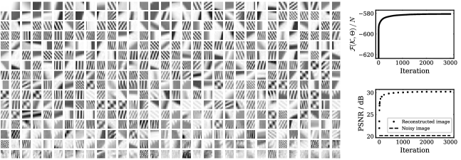
Figure 11: SSSC generative fields learned from the noisy “Barbara” image (compare Section 4.2). The fields are ordered according to their activation, starting with the fields corresponding to the most active hidden units.

Appendix G Evaluation Criteria

A standard metric for the evaluation of image restoration (IR) methods is the peak-signal-to-noise ratio (PSNR; compare Section 4). In the context of IR benchmarks (e.g., denoising, inpainting, image super resolution), PSNR values are informative about the root-mean-square error between the restored image calculated by a specific IR algorithm and the respective clean target image. In addition to the PSNR measure, there are other criteria that can be used to compare IR approaches. Some criteria will be discussed in the following.

Clean data. Supervised learning-based IR methods such as the denoising and inpainting methods of category DE6 and respectively IN6 in Table 2 require external datasets with clean images for training. In contrast, sparse coding and dictionary learning approaches such as the methods from category DE1 and IN1 (including the generative model algorithms EBSC and ES3C) are trained exclusively on the corrupted data they aim to restore. The ability of learning solely from corrupted data is very valuable for scenarios in which clean data is not available or difficult to generate. Besides, the internal statistics of a test image were observed to be often more predictive than statistics learned from external datasets (compare Shocher et al., 2018). For deep neural networks, which often do require external clean training data, recent work seeks to provide methods to also allow them to be trained on noisy data alone (e.g. Lehtinen et al., 2018; Ulyanov et al., 2018; Krull et al., 2019). Further related work proposes methods for “zero-shot” super-resolution which can be trained exclusively on the corrupted test data (Shocher et al., 2018).

A priori information and robustness. For denoising, it is frequently assumed that a priori knowledge of the ground-truth noise level is available. For instace KSVD, BM3D, WNNM, cKSVD or LSSC treat the noise level as input parameter of the algorithm. Other approaches that are trained using pairs of noisy/clean examples are typically optimized either for a single noise level (e.g. MLP, IRCNN, DnCNN-S, TNRD) or for several noise levels (e.g., MemNet, DnCNN-B, FFDNet, DPDNN, BDGAN). The denoising performance of noise-level-optimized approaches may deteriorate significantly if the algorithm is not provided with the appropriate (ground-truth) noise level of the test image (compare, e.g., Burger et al., 2012; Chaudhury and Roy, 2017; Zhang et al., 2018).

Similarly, for inpainting, it can be observed that certain methods exploit significant amounts of a priori information, for example considering the text removal benchmark (Figure 7 F): For NLRMRF and IRCNN, the training data is generated by overlaying specific text patterns on clean images. For IRCNN, several distinct font styles and font sizes are used (Chaudhury and Roy, 2017); for NLRMRF, training examples are generated using the identical text pattern of the test image (Sun and Tappen, 2011). In contrast, the generative model algorithms EBSC and ES3C require neither task-specific external training datasets (such as IRCNN or NLRMRF) nor do they require a-priori knowledge of the noise level (in contrast to e.g. BM3D, MLP, IRCNN, FFDNET, DnCNN; compare Table 2). EBSC and ES3C learn the noise level parameter (which is part of the generative model) from the data in an unsupervised way.

Context information. Another criterion for the evaluation of IR methods is the amount of context information that a particular algorithm exploits. The amount of context information is primarily determined by the patch size of the image segmentation. Increasing the effective patch size was reported to be beneficial for the performance of IR algorithms (compare Burger et al., 2012; Zhang et al., 2017). Zhang et al. reported that the effective patch size used by denoising methods can be found to vary greatly between different approaches (e.g. $36\times 36$ used by EPLL, $50\times 50$ by DnCNN-B, $70\times 70$ by FFDNet, $361\times 361$ by WNNM; numbers taken from Zhang et al., 2017, 2018). The denoising experiments with EBSC and ES3C were conducted using patches that did not exceed an effective size of $23\times 23$ (compare Table 3 in Appendix E) which is considerably smaller than the numbers reported by Zhang et al..

Stochasticity in the acquisition of test data. For the denoising benchmarks considered in Section 4.2, there is stochastic variation in the test data due to the fact that for a given AWG noise level $\sigma$ and for a given image, different realizations of the noise result in different noisy images. PSNR values can consequently vary even if the applied algorithm is fully deterministic. As all images investigated here are at least of size $256\times{}256$, variations due to different noise realizations are commonly taken as negligible for comparison (see, e.g., Mairal et al., 2009). The denoising results of EBSC and ES3C reported in Figures 5 and 6 were obtained by executing the algorithm three times on each image using different noise realizations in each run. Observed PSNR standard deviations were smaller or equal 0.06 dB (compare Table 4). For the inpainting experiments with randomly missing values (Figure 7 A-E), we also performed three runs for each image using a different realization of missing values in each run. In these experiments, we observed slightly higher PSNR variations (standard deviations ranged from 0.02 to 0.18 dB). The different realizations of the noise (or of the missing values) employed for each execution of the algorithm might be relevant to explain the PSNR variations we observed. Stochasticity in the EBSC and ES3C algorithms themselves however cannot be excluded as an additional factor.

Stochasticity in the algorithm. The output of stochastic algorithms can differ from run to run even if the input remains constant. For learning algorithms, different PSNR values usually correspond to different optima of the learning objective which are obtained due to different initializations and/or due to stochasticity during learning. For stochastic algorithms, it is therefore the question which PSNR value shall be used for comparison. Only two of the algorithms we used for comparison in Figures 5 - 7 report averages over different runs (KSVD and LSSC). All other algorithms do report a single PSNR value per denoising/inpainting setting without values for standard deviations. A single PSNR value is (for one realization of the corrupted image) naturally obtained for deterministic algorithms (e.g. BM3D, WNNM, NL). For the stochastic algorithms, a single PSNR may mean that either (A) just one run of the learning algorithm was performed, that (B) the best PSNR of all runs was reported, or that (C) one run of the learning algorithm was selected via another criterion. For DNN algorithms, for instance, the DNN with the lowest training or validation error could be selected for denoising or inpainting. Or for sparse coding algorithms, the model parameters with the lowest (approximate) likelihood could be selected for denoising or inpainting. As the contributions in Figure 5 - 7 which state just one PSNR value do not give details on how it was obtained from potentially several runs, it may be assumed that the best performing runs were reported (or sometimes the only run, e.g., in cases of a DNN requiring several days or weeks for training, compare Jain and Seung 2009; Burger et al. 2012; Chaudhury and Roy 2017; Zhang et al. 2018). Stating the best run is instructive as it shows how well an algorithm can perform under best conditions. For comparability, it should be detailed how the single PSNR value was selected, however (or if average and best values are essentially identical).

For practical applications, it is desirable to be able to select the best of several runs based on a criterion that can be evaluated without ground-truth knowledge. Our experimental data shows that for EBSC and ES3C the best denoising and inpainting performance in terms of PSNR cannot reliably be determined based on the learning objective, namely the variational bound (which is computable without ground-truth knowledge): The PSNR values of the runs with the highest bound may be smaller than the highest PSNR values observed in all runs. In a scenario with fixed noise realization, we observed the variational bound to be instructive about the PSNR value though (Figure 4).

Appendix H Comparison to GANs and VAEs

While Figures 5 to 7 show a comparison of EBSC and ES3C with a range of other denoising and inpainting approaches, no competitive performance for GANs and VAEs, except for BDGAN, is shown. Recent VAE versions instead frequently report approximate log-likelihoods on (binarized or standard) MNIST or human face datasets such as CelebA (e.g., Im et al., 2017; Creswell and Bharath, 2018). Creswell and Bharath also report reconstruction performance on AWG noise removal tasks, however in Creswell and Bharath (2018) (i) the considered noise levels are significantly smaller than the ones in Figures 5 - 6 and (ii) datasets such as Omniglot or CelebA are employed rather than the standard test images of Figures 5 - 6. Related contributions on GANs frequently consider the task of semantic inpainting, i.e. the reconstruction of large areas in images in a semantically plausible way (see, e.g., Cao et al., 2018, for an overview). In these contributions, typically datasets such as CelebA, Street View House Numbers images or ImageNet are employed and frequently the reconstruction of a single or a few (e.g. squared or rectangular) holes is considered as a benchmark (compare, e.g., Pathak et al., 2016; Yang et al., 2017; Yeh et al., 2017; Iizuka et al., 2017; Li et al., 2017). Yeh et al. also consider the task of restoring randomly missing values, however neither Yeh et al. (2017) nor the aforementioned publications report performance on the test images of Figure 7. The benchmarks of denoising and inpainting we use (Figures 5 to 7) are (A) very natural for EEM because of available benchmark results for mean field and sampling approaches, and (B) the benchmarks allow for comparison with state-of-the-art feed-forward DNNs (Figures 5 and 6).

References

- Ahmadi and Salari (2016) Kaveh Ahmadi and Ezzatollah Salari. Single-image super resolution using evolutionary sparse coding technique. IET Image Processing, 11(1):13–21, 2016.
- Angelino et al. (2016) Elaine Angelino, Matthew James Johnson, and Ryan P Adams. Patterns of scalable Bayesian inference. Foundations and Trends in Machine Learning, 9(2-3):119–247, 2016.
- Bell and Sejnowski (1997) A. J. Bell and T. J. Sejnowski. The “independent components” of natural scenes are edge filters. Vision Research, 37(23):3327–38, 1997.
- Bigdeli et al. (2020) Siavash A Bigdeli, Geng Lin, Tiziano Portenier, L Andrea Dunbar, and Matthias Zwicker. Learning Generative Models using Denoising Density Estimators. arXiv preprint arXiv:2001.02728, 2020.
- Blei et al. (2003) David M Blei, Andrew Y Ng, and Michael I Jordan. Latent Dirichlet Allocation. Journal of Machine Learning Research, 3:993–1022, 2003.
- Bouchard-Côté and Jordan (2009) Alexandre Bouchard-Côté and Michael I Jordan. Optimization of structured mean field objectives. In Proceedings of the Twenty-Fifth Conference on Uncertainty in Artificial Intelligence, pages 67–74, 2009.
- Burger et al. (2012) Harold C Burger, Christian J Schuler, and Stefan Harmeling. Image denoising: Can plain Neural Networks compete with BM3D? In CVPR, pages 2392–2399. IEEE, 2012.
- Cao et al. (2018) Yang-Jie Cao, Li-Li Jia, Yong-Xia Chen, Nan Lin, Cong Yang, Bo Zhang, Zhi Liu, Xue-Xiang Li, and Hong-Hua Dai. Recent Advances of Generative Adversarial Networks in Computer Vision. IEEE Access, 2018.
- Chaudhury and Roy (2017) Subhajit Chaudhury and Hiya Roy. Can fully convolutional networks perform well for general image restoration problems? In International Conference on Machine Vision Applications, pages 254–257, 2017.
- Chen and Pock (2017) Yunjin Chen and Thomas Pock. Trainable nonlinear reaction diffusion: A flexible framework for fast and effective image restoration. TPAMI, 39(6):1256–1272, 2017.
- Creswell and Bharath (2018) Antonia Creswell and Anil Anthony Bharath. Denoising Adversarial Autoencoders. IEEE Transactions on Neural Networks and Learning Systems, 30(4):968–984, 2018.
- Dabov et al. (2007) Kostadin Dabov, Alessandro Foi, Vladimir Katkovnik, and Karen Egiazarian. Image denoising by sparse 3D transform-domain collaborative filtering. IEEE Transactions on Image Processing, 16(8):2080–2095, 2007.
- Dai and Lücke (2014) Z. Dai and J. Lücke. Autonomous Document Cleaning – A Generative Approach to Reconstruct Strongly Corrupted Scanned Texts. TPAMI, 36(10):1950–1962, 2014.
- Dalcín et al. (2005) Lisandro Dalcín, Rodrigo Paz, and Mario Storti. MPI for Python. Journal of Parallel and Distributed Computing, 65(9):1108 – 1115, 2005.
- Dayan et al. (1995) Peter Dayan, Geoffrey E. Hinton, Radford Neal, and Richard S. Zemel. The Helmholtz machine. Neural Computation, 7:889 – 904, 1995.
- Dinh et al. (2014) Laurent Dinh, David Krueger, and Yoshua Bengio. Nice: Non-linear independent components estimation. arXiv:1410.8516, 2014.
- Dinh et al. (2017) Laurent Dinh, Jascha Sohl-Dickstein, and Samy Bengio. Density Estimation using Real NVP. In ICLR, 2017.
- Dong et al. (2019) W. Dong, P. Wang, W. Yin, G. Shi, F. Wu, and X. Lu. Denoising Prior Driven Deep Neural Network for Image Restoration. TPAMI, 2019.
- Elad and Aharon (2006) M. Elad and M.l Aharon. Image Denoising Via Sparse and Redundant Representations Over Learned Dictionaries. IEEE Transactions on Image Processing, 15(12):3736–3745, 2006.
- Exarchakis and Lücke (2017) G. Exarchakis and J. Lücke. Discrete Sparse Coding. Neural Computation, 29:2979–3013, 2017.
- Fadili and Starck (2005) Jalal M Fadili and Jean-Luc Starck. Sparse representations and Bayesian image inpainting. In Proceedings of International Conferences SPARS’05, page 4 pp, 2005.
- Földiák (1990) P. Földiák. Forming sparse representations by local anti-Hebbian learning. Biological Cybernetics, 64:165–170, 1990.
- Forster and Lücke (2018) Dennis Forster and Jörg Lücke. Can clustering scale sublinearly with its clusters? A variational EM acceleration of GMMs and k-means. In AISTATS, pages 124–132, 2018.
- Forster et al. (2018) Dennis Forster, Abdul-Saboor Sheikh, and Jörg Lücke. Neural Simpletrons: Learning in the Limit of Few Labels with Directed Generative Networks. Neural Computation, 30(8):2113–2174, 2018.
- Ghahramani and Jordan (1995) Zoubin Ghahramani and Michael I Jordan. Learning from incomplete data. 1995. A.I. Memo No. 1509.
- Goldberg (2006) David E Goldberg. Genetic Algorithms. Pearson Education India, 2006.
- Goodfellow et al. (2012) Ian Goodfellow, Aaron C. Courville, and Yoshua Bengio. Large-Scale Feature Learning With Spike-and-Slab Sparse Coding. In ICML, 2012.
- Goodfellow et al. (2014) Ian Goodfellow, Jean Pouget-Abadie, Mehdi Mirza, Bing Xu, David Warde-Farley, Sherjil Ozair, Aaron Courville, and Yoshua Bengio. Generative Adversarial Nets. In NIPS. 2014.
- Gu et al. (2014) Shuhang Gu, Lei Zhang, Wangmeng Zuo, and Xiangchu Feng. Weighted Nuclear Norm Minimization with Application to Image Denoising. In CVPR, pages 2862–2869. IEEE, 2014.
- Guiraud et al. (2018) E. Guiraud, J. Drefs, and J. Lücke. Evolutionary Expectation Maximization. In GECCO, 2018.
- Gupta and Chen (2011) Maya R Gupta and Yihua Chen. Theory and use of the em algorithm. Foundations and Trends® in Signal Processing, 4(3):223–296, 2011.
- Haft et al. (2004) M. Haft, R. Hofman, and V. Tresp. Generative binary codes. Formal Pattern Analysis & Applications, 6:269–84, 2004.
- Henniges et al. (2010) M. Henniges, G. Puertas, J. Bornschein, J. Eggert, and J. Lücke. Binary Sparse Coding. In LVA/ICA, pages 450–57. Springer, 2010.
- Hoyer (2003) Patrik O. Hoyer. Modeling receptive fields with non-negative sparse coding. Neurocomputing, 52-54:547–52, 2003.
- Hruschka et al. (2009) Eduardo Raul Hruschka, Ricardo JGB Campello, Alex A Freitas, et al. A survey of evolutionary algorithms for clustering. IEEE Transactions on Systems, Man, and Cybernetics, 39(2):133–155, 2009.
- Huang et al. (2018) Chin-Wei Huang, David Krueger, Alexandre Lacoste, and Aaron Courville. Neural Autoregressive Flows. In ICML, 2018.
- Hughes and Sudderth (2016) Michael C Hughes and Erik B Sudderth. Fast Learning of Clusters and Topics via Sparse Posteriors. arXiv preprint arXiv:1609.07521, 2016.
- Hyvärinen and Pajunen (1999) A. Hyvärinen and P. Pajunen. Nonlinear Independent Component Analysis: Existence and uniqueness results. Neural Networks, 12(3):429–439, 1999.
- Iizuka et al. (2017) Satoshi Iizuka, Edgar Simo-Serra, and Hiroshi Ishikawa. Globally and Locally Consistent Image Completion. ACM Transactions on Graphics (ToG), 36(4):1–14, 2017.
- Ilin and Valpola (2005) A. Ilin and H. Valpola. On the effect of the form of the posterior approximation in variational learning of ICA models. Neural Processing Letters, 22(2):183–204, 2005.
- Im et al. (2017) Daniel Im Jiwoong Im, Sungjin Ahn, Roland Memisevic, and Yoshua Bengio. Denoising Criterion for Variational Auto-Encoding Framework. In AAAI Conference on Artificial Intelligence, 2017.
- Imamura et al. (2019) Ryuji Imamura, Tatsuki Itasaka, and Masahiro Okuda. Zero-Shot Hyperspectral Image Denoising With Separable Image Prior. In IEEE International Conference on Computer Vision Workshop, 2019.
- Jain and Seung (2009) Viren Jain and Sebastian Seung. Natural Image Denoising with Convolutional Networks. In NIPS, 2009.
- Jernite et al. (2013) Yacine Jernite, Yonatan Halpern, and David Sontag. Discovering Hidden Variables in Noisy-Or Networks using Quartet Tests. In NIPS, 2013.
- Jordan et al. (1999) M. Jordan, Z. Ghahramani, T. Jaakkola, and L. Saul. An introduction to variational methods for graphical models. Machine Learning, 37:183–233, 1999.
- Kingma and Welling (2014) Diederik P Kingma and Max Welling. Auto-Encoding Variational Bayes. In ICLR, 2014.
- Kingma and Dhariwal (2018) Durk P Kingma and Prafulla Dhariwal. Glow: Generative flow with invertible 1x1 convolutions. In NIPS, 2018.
- Kingma et al. (2016) Durk P Kingma, Tim Salimans, Rafal Jozefowicz, Xi Chen, Ilya Sutskever, and Max Welling. Improved Variational Inference with Inverse Autoregressive Flow. In NIPS, 2016.
- Krull et al. (2019) Alexander Krull, Tim-Oliver Buchholz, and Florian Jug. Noise2Void - Learning Denoising From Single Noisy Images. In Proceedings of the IEEE Conference on Computer Vision and Pattern Recognition, pages 2129–2137, 2019.
- Lee et al. (2007) H. Lee, A. Battle, R. Raina, and A. Ng. Efficient sparse coding algorithms. In NIPS, volume 20, pages 801–08, 2007.
- Lehtinen et al. (2018) Jaakko Lehtinen, Jacob Munkberg, Jon Hasselgren, Samuli Laine, Tero Karras, Miika Aittala, and Timo Aila. Noise2Noise: Learning image restoration without clean data. In ICML, volume 80, pages 2965–2974, 2018.
- Li (2008) Xin Li. Patch-based image interpolation: algorithms and applications. In International Workshop on Local and Non-Local Approximation in Image Processing, pages 1–6, 2008.
- Li et al. (2017) Yijun Li, Sifei Liu, Jimei Yang, and Ming-Hsuan Yang. Generative Face Completion. In CVPR, pages 3911–3919. IEEE, 2017.
- Little and Rubin (1987) Roderick JA Little and Donald B Rubin. Statistical Analysis with Missing Data. Wiley Series in Probability and Statistics. John Wiley & Sons, 1st edition, 1987.
- Loshchilov and Hutter (2016) Ilya Loshchilov and Frank Hutter. CMA-ES for Hyperparameter Optimization of Deep Neural Networks. In ICLR Workshop, pages 513–520, 2016.
- Lücke and Sahani (2008) J. Lücke and M. Sahani. Maximal causes for non-linear component extraction. Journal of Machine Learning Research, 9:1227–67, 2008.
- Lücke (2019) Jörg Lücke. Truncated Variational Expectation Maximization. arXiv preprint, arXiv:1610.03113, 2019.
- Lücke and Eggert (2010) Jörg Lücke and Julian Eggert. Expectation Truncation And the Benefits of Preselection in Training Generative Models. Journal of Machine Learning Research, 11:2855–900, 2010.
- Lücke and Forster (2019) Jörg Lücke and Dennis Forster. k-means as a variational EM approximation of Gaussian mixture models. Pattern Recognition Letters, 125:349–356, 2019.
- Lücke and Sheikh (2012) Jörg Lücke and Abdul-Saboor Sheikh. Closed-Form EM for Sparse Coding and Its Application to Source Separation. In LVA/ICA, pages 213–221, 2012.
- Lücke et al. (2018) Jörg Lücke, Zhenwen Dai, and Georgios Exarchakis. Truncated Variational Sampling for “Black Box” Optimization of Generative Models. In LVA/ICA, pages 467–478, 2018.
- MacKay (2003) D. J. C. MacKay. Information Theory, Inference, and Learning Algorithms. Cambridge University Press, 2003.
- Mackay (2001) David J. C. Mackay. Local minima, symmetry-breaking, and model pruning in variational free energy minimization. Inference Group, Cavendish Laboratory, Cambridge, UK, 2001.
- Mairal et al. (2009) J. Mairal, F. Bach, J. Ponce, G. Sapiro, and A. Zisserman. Non-Local Sparse Models for Image Restoration. International Conference on Computer Vision, 25, 2009.
- Mairal et al. (2008) Julien Mairal, Michael Elad, and Guillermo Sapiro. Sparse Representation for Color Image Restoration. IEEE Transactions on Image Processing, 17(1):53–69, 2008.
- Mohamed et al. (2012) S. Mohamed, K. Heller, and Z. Ghahramani. Evaluating Bayesian and L1 approaches for sparse unsupervised learning. In ICML, 2012.
- Murphy (2012) Kevin P Murphy. Machine Learning: A probabilistic perspective. MIT press, 2012.
- Myers et al. (1999) James W Myers, Kathryn B Laskey, and Kenneth A DeJong. Learning bayesian networks from incomplete data using evolutionary algorithms. In GECCO, 1999.
- Neal and Hinton (1998) Radford Neal and G. Hinton. A view of the EM algorithm that justifies incremental, sparse, and other variants. In M. I. Jordan, editor, Learning in Graphical Models. Kluwer, 1998.
- Oehmcke and Kramer (2018) Stefan Oehmcke and Oliver Kramer. Knowledge Sharing for Population Based Neural Network Training. In Joint German/Austrian Conference on Artificial Intelligence, pages 258–269, 2018.
- Olshausen and Field (1996) B. Olshausen and D. Field. Emergence of simple-cell receptive field properties by learning a sparse code for natural images. Nature, 381:607–9, 1996.
- Olshausen and Field (1997) Bruno A. Olshausen and David J. Field. Sparse coding with an overcomplete basis set: A strategy employed by V1? Vision Research, 37(23):3311–3325, 1997.
- Opper and Archambeau (2009) Manfred Opper and Cédric Archambeau. The variational Gaussian approximation revisited. Neural computation, 21(3):786–792, 2009.
- Opper and Winther (2005) Manfred Opper and Ole Winther. Expectation consistent approximate inference. Journal of Machine Learning Research, 6(Dec):2177–2204, 2005.
- Pathak et al. (2016) Deepak Pathak, Philipp Krahenbuhl, Jeff Donahue, Trevor Darrell, and Alexei A Efros. Context Encoders: Feature Learning by Inpainting. In CVPR, pages 2536–2544. IEEE, 2016.
- Pernkopf and Bouchaffra (2005) Franz Pernkopf and Djamel Bouchaffra. Genetic-based EM algorithm for learning Gaussian mixture models. TPAMI, 27(8):1344–1348, 2005.
- Prellberg and Kramer (2018) Jonas Prellberg and Oliver Kramer. Limited Evaluation Evolutionary Optimization of Large Neural Networks. In Joint German/Austrian Conference on Artificial Intelligence, pages 270–283, 2018.
- Ranganath et al. (2014) Rajesh Ranganath, Sean Gerrish, and David Blei. Black Box Variational Inference. In AISTATS, pages 814–822, 2014.
- Real et al. (2017) Esteban Real, Sherry Moore, Andrew Selle, Saurabh Saxena, Yutaka Leon Suematsu, Jie Tan, Quoc V. Le, and Alexey Kurakin. Large-scale evolution of image classifiers. In ICML, pages 2902–2911, 2017.
- Rezende and Mohamed (2015) Danilo Jimenez Rezende and Shakir Mohamed. Variational inference with normalizing flows. ICML, 2015.
- Rezende et al. (2014) Danilo Jimenez Rezende, Shakir Mohamed, and Daan Wierstra. Stochastic Backpropagation and Approximate Inference in Deep Generative Models. In ICML, 2014.
- Roth and Black (2009) Stefan Roth and Michael J. Black. Fields of experts. IJCV, 82(2):205, 2009.
- Rotmensch et al. (2017) M. Rotmensch, Y. Halpern, A. Tlimat, S. Horng, and D. Sontag. Learning a Health Knowledge Graph from Electronic Medical Records. Scientific Reports, 7(1):5994, 2017.
- Salimans et al. (2017) Tim Salimans, Jonathan Ho, Xi Chen, Szymon Sidor, and Ilya Sutskever. Evolution Strategies as a Scalable Alternative to Reinforcement Learning. arXiv preprint arXiv:1703.03864, 2017.
- Saul and Jordan (1996) Lawrence K Saul and Michael I Jordan. Exploiting tractable substructures in intractable networks. NIPS, 1996.
- Saul et al. (1996) Lawrence K Saul, Tommi Jaakkola, and Michael I Jordan. Mean Field Theory for Sigmoid Belief Networks. Journal of Artificial Intelligence Research, 4(1):61–76, 1996.
- Schmidt et al. (2010) Uwe Schmidt, Qi Gao, and Stefan Roth. A Generative Perspective on MRFs in Low-Level Vision. In CVPR, pages 1751–1758, 2010.
- Seeger (2008) M. Seeger. Bayesian inference and optimal design for the sparse linear model. Journal of Machine Learning Research, 9:759–813, 2008.
- Serra et al. (2017) Juan G Serra, Matteo Testa, Rafael Molina, and Aggelos K Katsaggelos. Bayesian K-SVD Using Fast Variational Inference. IEEE Transactions on Image Processing, 26(7):3344–3359, 2017.
- Sheikh and Lücke (2016) A.-S. Sheikh and J. Lücke. Select-and-Sample for Spike-and-Slab Sparse Coding. In NIPS, 2016.
- Sheikh et al. (2014) Abdul-Saboor Sheikh, Jacquelyn A. Shelton, and Jörg Lücke. A Truncated EM Approach for Spike-and-Slab Sparse Coding. Journal of Machine Learning Research, 15:2653–2687, 2014.
- Sheikh et al. (2019) Abdul-Saboor Sheikh, Nicol S. Harper, Jakob Drefs, Yosef Singer, Zhenwen Dai, Richard E. Turner, and Jörg Lücke. STRFs in primary auditory cortex emerge from masking-based statistics of natural sounds. PLOS Computational Biology, 15(1):e1006595, 2019.
- Shelton et al. (2011) J. A. Shelton, J. Bornschein, A.-S. Sheikh, P. Berkes, and J. Lücke. Select and Sample – A Model of Efficient Neural Inference and Learning. NIPS, 24:2618–2626, 2011.
- Shelton et al. (2017) Jacquelyn A Shelton, Jan Gasthaus, Zhenwen Dai, Jörg Lücke, and Arthur Gretton. GP-Select: Accelerating EM Using Adaptive Subspace Preselection. Neural Computation, 29(8):2177–2202, 2017.
- Shocher et al. (2018) Assaf Shocher, Nadav Cohen, and Michal Irani. “Zero-Shot” Super-Resolution using Deep Internal Learning. In CVPR, pages 3118–3126. IEEE, 2018.
- Singliar and Hauskrecht (2006) T. Singliar and M. Hauskrecht. Noisy-OR Component Analysis and its Application to Link Analysis. Journal of Machine Learning Research, 7:2189–2213, 2006.
- Stanley and Miikkulainen (2002) Kenneth O. Stanley and Risto Miikkulainen. Evolving neural networks through augmenting topologies. Evolutionary Computing, 10(2):99–127, 2002.
- Steinruecken et al. (2019) Christian Steinruecken, Emma Smith, David Janz, James Lloyd, and Zoubin Ghahramani. The Automatic Statistician. In Automated Machine Learning. Springer, 2019.
- Suganuma et al. (2017) Masanori Suganuma, Shinichi Shirakawa, and Tomoharu Nagao. A Genetic Programming Approach to Designing Convolutional Neural Network Architectures. In GECCO, 2017.
- Sun and Tappen (2011) Jian Sun and Marshall F Tappen. Learning Non-Local Range Markov Random field for Image Restoration. In CVPR, pages 2745–2752, 2011.
- Tai et al. (2017) Ying Tai, Jian Yang, Xiaoming Liu, and Chunyan Xu. Memnet: A persistent memory network for image restoration. In CVPR, pages 4539–4547. IEEE, 2017.
- Tian et al. (2020) Chunwei Tian, Yong Xu, and Wangmeng Zuo. Image denoising using deep CNN with batch renormalization. Neural Networks, 121:461–473, 2020.
- Tian et al. (2011) GuangJian Tian, Yong Xia, Yanning Zhang, and Dagan Feng. Hybrid genetic and variational expectation-maximization algorithm for gaussian-mixture-model-based brain mr image segmentation. IEEE Transactions on Information Technology in Biomedicine, 15(3):373–380, 2011.
- Titsias and Lázaro-Gredilla (2011) Michalis K. Titsias and Miguel Lázaro-Gredilla. Spike and Slab Variational Inference for Multi-Task and Multiple Kernel Learning. In NIPS, 2011.
- Tohka et al. (2007) Jussi Tohka, Evgeny Krestyannikov, Ivo D Dinov, Allan MacKenzie Graham, David W Shattuck, Ulla Ruotsalainen, and Arthur W Toga. Genetic algorithms for finite mixture model based voxel classification in neuroimaging. IEEE Transactions on Medical Imaging, 26(5):696–711, 2007.
- Turner and Sahani (2011) R. E. Turner and M. Sahani. Bayesian Time Series Models, chapter Two problems with variational expectation maximisation for time-series models. Cambridge Univ Press, 2011.
- Ulyanov et al. (2018) Dmitry Ulyanov, Andrea Vedaldi, and Victor Lempitsky. Deep Image Prior. In Proceedings of the IEEE Conference on Computer Vision and Pattern Recognition, pages 9446–9454, 2018.
- van Hateren and van der Schaaf (1998) J. H. van Hateren and A. van der Schaaf. Independent component filters of natural images compared with simple cells in primary visual cortex. Proceedings of the Royal Society of London. Series B: Biological Sciences, 265:359–66, 1998.
- Vértes and Sahani (2018) Eszter Vértes and Maneesh Sahani. Flexible and accurate inference and learning for deep generative models. In NIPS, 2018.
- Yang et al. (2017) Chao Yang, Xin Lu, Zhe Lin, Eli Shechtman, Oliver Wang, and Hao Li. High-Resolution Image Inpainting using Multi-Scale Neural Patch Synthesis. In CVPR, pages 6721–6729. IEEE, 2017.
- Yeh et al. (2017) Raymond A Yeh, Chen Chen, Teck Yian Lim, Alexander G Schwing, Mark Hasegawa-Johnson, and Minh N Do. Semantic Image Inpainting with Deep Generative Models. In CVPR, pages 5485–5493. IEEE, 2017.
- Yu et al. (2012) Guoshen Yu, Guillermo Sapiro, and Stéphane Mallat. Solving Inverse Problems With Piecewise Linear Estimators: From Gaussian Mixture Models to Structured Sparsity. IEEE Transactions on Image Processing, 21(5):2481–2499, 2012.
- Zhang et al. (2017) Kai Zhang, Wangmeng Zuo, Yunjin Chen, Deyu Meng, and Lei Zhang. Beyond a Gaussian Denoiser: Residual Learning of Deep CNN for Image Denoising. IEEE Transactions on Image Processing, 26(7):3142–3155, 2017.
- Zhang et al. (2018) Kai Zhang, Wangmeng Zuo, and Lei Zhang. FFDNet: Toward a fast and flexible solution for CNN based image denoising. IEEE Transactions on Image Processing, 2018.
- Zhou et al. (2009) M. Zhou, H. Chen, J. Paisley, L. Ren, G. Sapiro, and L. Carin. Non-Parametric Bayesian Dictionary Learning for Sparse Image Representations. In NIPS, 2009.
- Zhou et al. (2012) Mingyuan Zhou, Haojun Chen, John Paisley, Lu Ren, Lingbo Li, Zhengming Xing, David Dunson, Guillermo Sapiro, and Lawrence Carin. Nonparametric Bayesian Dictionary Learning for Analysis of Noisy and Incomplete Images. IEEE Transactions on Image Processing, 21(1):130–144, 2012.
- Zhu et al. (2019) Shipeng Zhu, Guili Xu, Yuehua Cheng, Xiaodong Han, and Zhengsheng Wang. BDGAN: Image Blind Denoising Using Generative Adversarial Networks. In Chinese Conference on Pattern Recognition and Computer Vision, pages 241–252, 2019.
- Zoran and Weiss (2011) Daniel Zoran and Yair Weiss. From Learning Models of Natural Image Patches to Whole Image Restoration. In IEEE International Conference on Computer Vision, pages 479–486, 2011.