The VMC Survey – XL. Three-dimensional structure of the Small Magellanic Cloud as derived from red clump stars

Abstract

Galaxy interactions distort the distribution of baryonic matter and can affect star formation. The nearby Magellanic Clouds are a prime example of an ongoing galaxy interaction process. Here we use the intermediate-age ($\sim 1$–$10$ Gyr) red clump stars to map the three-dimensional structure of the Small Magellanic Cloud (SMC) and interpret it within the context of its history of interaction with the Large Magellanic Cloud (LMC) and the Milky Way. Red clump stars are selected from near-infrared colour–magnitude diagrams based on data from the VISTA survey of the Magellanic Clouds. Interstellar reddening is measured and removed, and the corrected brightness is converted to a distance, on a star-by-star basis. A flat plane fitted to the spatial distribution of red clump stars has an inclination $i=35\degr$–$48\degr$ and position angle PA$=170\degr$–$186\degr$. However, significant deviations from this plane are seen, especially in the periphery and on the eastern side of the SMC. In the latter part, two distinct populations are present, separated in distance by as much as 10 kpc. Distant red clump stars are seen in the North of the SMC, and possibly also in the far West; these might be associated with the predicted ‘Counter-Bridge’. We also present a dust reddening map, which shows that dust generally traces stellar mass. The structure of the intermediate-age stellar component of the SMC bears the imprints of strong interaction with the LMC a few Gyr ago, which cannot be purely tidal but must have involved ram pressure stripping.

1 Introduction

The details of how galaxies have evolved over cosmological times are imprinted in their star formation history (SFH), chemical enrichment, and morphological and kinematic structure. Many galaxies have experienced interactions with other galaxies, and this will have affected their evolution. If we are to understand galaxy evolution, we need to understand what happens during galaxy interactions. A prime example of a galaxy interaction is found in our backyard – the Magellanic System, comprising the Large Magellanic Cloud (LMC) and the Small Magellanic Cloud (SMC) at distances of just $\approx 50$ kpc (LMC; de Grijs et al., 2014) and $\approx 61$ kpc (SMC; de Grijs & Bono, 2015), the Magellanic Bridge between them, the purely gaseous Magellanic Stream trailing them, and the Leading Arm ahead of them in their flight through the Milky Way halo. In this paper we investigate the structure of the SMC as seen in its intermediate-age ($\sim 1$–$10$ Gyr) red-clump stars and link it to the recent LMC–SMC–Milky Way interaction history.

While their three-dimensional (3-D) space motions have been used to argue that the Magellanic Clouds are on their first close passage of the Milky Way, this is not certain and depends on the Milky Way’s mass (Kallivayalil et al., 2013; Patel et al., 2017). In any case, mutual interactions between the LMC and SMC may have occurred more often and over a longer period of time (Besla et al., 2016). Gradients in gravity and momentum have led to tidal stretching and bending, most notably in the form of an eastern extension to the SMC known as the ‘Wing’ (Shapley, 1940; Gonidakis et al., 2009; Belokurov & Erkal, 2019); this is now also seen in the internal kinematics (e.g., Niederhofer et al., 2018). While the Bridge is for certain a result of the galaxy interactions, too, it has proven to be a more complex structure than initially thought, with different distributions of gas (Hindman et al., 1963), young stars (Irwin et al., 1990) and old stars (Belokurov et al., 2017). The existence of the Magellanic Stream as well as recent proper motion measurements of stars within the SMC both indicate that a physical collision has happened between the LMC and SMC $\sim 200$ Myr ago (Hammer et al., 2015; Zivick et al., 2018).

Table 1: Line-of-sight depths for the SMC from the literature.

Publication	Depth (kpc)	Notes
Hatzidimitriou & Hawkins (1989)	17, 7	$2\sigma$ North–East and South–West
Gardiner & Hawkins (1991)	4–16	$2\sigma$ depth dependent on portion observed (North and North–West)
Groenewegen (2000)	14	(OGLE-II, DENIS and 2MASS) Cepheids, front–back
Crowl et al. (2001)	$(4.1\pm 0.8)$–$(6.3\pm 1.3)$	Cepheids
Glatt et al. (2008)	$\sim 10$	deep Hubble Space Telescope imaging
Subramanian & Subramaniam (2009)	$3.4\pm 1.2$	OGLE-II RC: average depth of the disc
Subramanian & Subramaniam (2009)	$4.2\pm 1.0$	OGLE-II RC: average depth in the North
Subramanian & Subramaniam (2009)	$2.6\pm 0.8$	OGLE-II RC: average depth in the South
Subramanian & Subramaniam (2009)	$3.1\pm 1.0$	OGLE-II RC: average depth in the East
Subramanian & Subramaniam (2009)	$2.8\pm 0.9$	OGLE-II RC: average depth in the West
Kapakos et al. (2011)	$4.13\pm 0.27$	OGLE-II/III RR Lyræ V-band: Central area $1\sigma$
Haschke et al. (2012)	$4.2\pm 0.4$	OGLE-III RR Lyræ
Haschke et al. (2012)	5.14–6.02	OGLE-III Cepheids; dependent on field selection
Kapakos & Hatzidimitriou (2012)	$5.3\pm 0.4$	OGLE-II/III RR Lyræ V-band: Extended region $1\sigma$
Subramanian & Subramaniam (2012)	$4.57\pm 1.03$	$1\sigma$ OGLE-III RC stars
Subramanian & Subramaniam (2012)	6–8	$1\sigma$ OGLE-III RC stars (North–Eastern regions)
Subramanian & Subramaniam (2012)	$\sim 14$	$4\sigma$ OGLE-III RR Lyræ & RC stars front to back
Subramanian & Subramaniam (2015)	$8.1\pm 1.4$	OGLE-III SMC disc $z$-distribution
Subramanian & Subramaniam (2015)	$1.8\pm 0.6$	OGLE-III SMC disc orientation corrected
Deb et al. (2015)	$4.9\pm 0.7$	OGLE-III RR Lyræ (RRab); Fourier relation
Deb et al. (2015)	$4.1\pm 0.7$	OGLE-III RR Lyræ (RRab); metallicity relation

Table 2: Position angle (PA) and inclination ($i$) for the SMC from the literature.

Publication	$i$ ($\degr$)	PA ($\degr$)	Notes
Caldwell & Coulson (1986)	$70\pm 3$	$58\pm 10$	Cepheids
Laney & Stobie (1986)	$45\pm 7$	$55\pm 17$	Cepheids
Groenewegen (2000)	$68\pm 2$	$238\pm 7$*	(OGLE-II, 2MASS and DENIS) Cepheids
Kunkel et al. (2000)	$73\pm 4$		Radial velocities Carbon stars
Stanimirović et al. (2004)	$40\pm 20$	$40\pm 10$	H i
Haschke et al. (2012)	$74\pm 9$	$66\pm 15$	OGLE-III Cepheids
Haschke et al. (2012)	$7\pm 15$	$83\pm 21$	OGLE-III RR Lyræ
Subramanian & Subramaniam (2012)	0.58	55.5	OGLE-III RC axes ratio
Subramanian & Subramaniam (2012)	0.50	58.3	OGLE-III RR Lyræ axis
Dobbie et al. (2014)	25–70	120–130	Radial velocities RGB stars
Deb et al. (2015)	$2.3\pm 0.8$	$74.3\pm 0.5$	OGLE-III RRab stars
Deb et al. (2015)	$0.51\pm 0.29$	$56.0\pm 0.8$	OGLE-III Main body
Deb et al. (2015)	$2.244\pm 0.024$	$85.54\pm 0.33$	OGLE-III North–Eastern arm
Subramanian & Subramaniam (2015)	$63.1\pm 1.0$	$152\pm 8$	OGLE-III Cepheids fundamental-mode
Subramanian & Subramaniam (2015)	$66.3\pm 0.9$	$159\pm 10$	OGLE-III Cepheids first-overtone
Subramanian & Subramaniam (2015)	$64.4\pm 0.7$	$155\pm 6$	OGLE-III Cepheids combined
Rubele et al. (2015)	$39.3\pm 5.5$	$179.3\pm 2.1$	CMDs
Deb (2017)	$2.30\pm 0.14$	$38.5\pm 0.3$	OGLE-IV RRab stars
Deb (2017)	$3.16\pm 0.19$	$38.0\pm 0.6$	OGLE-IV RRab stars
*Subtracting $180\degr$ from this PA brings it in line with the other results.

There exists a rich history of line-of-sight depth measurements in the SMC, motivated by large values of 20–30 kpc in the eastern part inferred from Cepheid variables distance measurements by Mathewson et al. (1986, 1988) (cf. Hatzidimitriou et al., 1993). Stanimirović et al. (2004) reviewed these findings (see also the more recent review by de Grijs & Bono, 2015), noting that Zaritsky et al. (2002) had mentioned that differential interstellar extinction can lead to Cepheid distances being overestimated. Correction for this would bring most values down to within the tidal radius (4–9 kpc). Even at the time Welch et al. (1987) pointed out flaws with these measurements. Further line-of-sight depth determinations are listed in Table 1, where some (e.g., Haschke et al., 2012) have interpreted the Crowl et al. (2001) data as a 6–12 kpc depth. Kapakos et al. (2011) argued that the metal-rich stars form a thin disc-like structure whilst the metal-poor stars form a halo- or bulge-like structure, appearing thicker in the North–East (see also Kapakos & Hatzidimitriou, 2012).

Measurements of the orientation of the SMC are challenging due to the stretched nature of the Wing, an elongated young main body and the ellipsoidal shape of the old population. This is reflected in a large variance in position angle (PA) and inclination ($i$) values (see Table 2). A clear age dichotomy is seen, with young stellar populations ($<1$ Gyr; Cepheids) steeply inclined with respect to the plane of the sky while old populations ($>10$ Gyr; RR Lyræ) are shallower. Haschke et al. (2012) suggested that this difference is due to interactions with the LMC and Milky Way. This must mean that ram pressure on the gas played a role in the interactions, as tidal forces alone would not differentiate between stars of different ages (nor between gas and stars). Alternatively, a dwarf–dwarf galaxy merger early on in the evolution of the SMC could have resulted in a spheroidal old component and a rotating gaseous disc that has since been truncated by interactions with the LMC (Bekki & Chiba, 2008). The merger scenario would predict an intermediate-age component to be disc like. Furthermore, the main body of the SMC is less inclined than its periphery; this has been explained as due to tidal forces between the LMC and SMC (Deb et al., 2015). The range of position angles is much smaller in the main body of the SMC than in other regions and this variance suggests the SMC is not a flat disc.

In this work, we use red clump (RC) stars as tracers of the 3-D structure of the SMC. RC stars form a metal-rich, younger counterpart to the horizontal branch. Stars in this phase of stellar evolution are of low mass ($<2.2$ M_⊙) and undergo core helium and shell hydrogen burning, starting at an almost-fixed core mass and hence luminosity (Girardi, 2016). Following the first ascent of the red giant branch (RGB) the RC phase typically lasts $\sim 0.1$ Gyr (up to 0.2 Gyr). As a result RC stars are easily noticeable in colour–magnitude diagrams (CMDs) as a clump of stars close to the RGB (Salaris, 2012, their Figure 4). As standard candles and more numerous than variable stars such as RR Lyræ and Cepheids, RC stars are choice tracers of intermediate-age (a few Gyr) stellar populations in galaxies with recent/ongoing star formation (Girardi & Salaris, 2001). Their ages imply they have had sufficient time to mix well dynamically as, in the absence of strong rotational support or external influences, an SMC-like dwarf galaxy would virialise within a few crossing times (well within a Gyr) into a spheroidal configuration; morphological and kinematical distortions must in general be due to tidal forces resulting from galaxy interactions. Comparisons with maps obtained using younger Cepheids (Jacyszyn-Dobrzeniecka et al., 2016; Scowcroft et al., 2016; Ripepi et al., 2017) and older RR Lyræ (Jacyszyn-Dobrzeniecka et al., 2017; Muraveva et al., 2018) can then place these results in a galactic evolutionary context, as was done for the 2-D case by Cioni et al. (2000), Zaritsky et al. (2000) and Sun et al. (2018).

The studies of SMC depth and structure in general, are hampered by attenuation of starlight by dust in the interstellar medium (ISM) and its wavelength dependence (Gieren et al., 2013). The effect is smaller in the infrared (IR) than in the optical and we therefore chose to make use of near-IR data. Still, it can be significant relative to the accuracy we aim to achieve ($\Delta m\sim 0.03$ mag) to trace small differences in distance ($\Delta d<1$ kpc). We therefore determine the amount of reddening and attenuation and correct for it. As a by-product, we obtain a map of the interstellar dust distribution, which traces the ISM and can be compared with the stellar distribution – see Tatton et al. (2013) for an application to the area around 30 Doradus in the LMC.

The structure of this paper is as follows. Section 2 describes the data used; Section 3 describes the RC star selection and de-reddening procedures; Section 4 presents the reddening map; Section 5 presents the derived 3-D structure; we discuss the results in Section 6 and conclude the paper in Section 7.

2 Data

We used near-IR $Y$ and $K_{\rm s}$ photometry from images taken with the Visible and Infrared Survey Telescope for Astronomy (VISTA; Sutherland et al., 2015) as part of the VISTA Survey of the Magellanic Clouds (VMC; Cioni et al., 2011). These data were obtained with the VISTA Infrared Camera (VIRCAM; Sutherland et al., 2015) and processed with the VISTA Data Flow System (VDFS; Irwin et al., 2004; González-Fernández et al., 2018). The exposure times were 40 min. for the $Y$ band and 150 min. for the $K_{\rm s}$ band. The 50% completeness level is reached at $K_{\rm s}>20$ mag (Rubele et al., 2015), varying with local crowding levels. The stars we study in this work are brighter than $K_{\rm s}=19.5$ mag, where completeness is always $>90$%.

The data used covers the entire VMC survey area for the SMC, encompassing 27 SMC tiles (each covering almost uniformly an area of 1.5 deg² in which each pixel received at least two exposures; Sutherland et al., 2015). Figure 1 shows a source density map of the SMC for the $K_{\rm s}=16$–18 mag range. All coordinates quoted throughout this paper are J2000. The gap between tiles SMC 5_3 and SMC 5_4 (RA $=13\hbox to0.0pt{.\hss}{\degr}5$ Dec $=-72\degr$) is the result of the automatic centring of each tile in order to include a sufficient number of guide stars (the gap is being covered with new VISTA observations). One of the tiles could not be used in full (SMC 5_2; centred at RA $=6\hbox to0.0pt{.\hss}{\degr}7$, Dec $=-71\hbox to0.0pt{.\hss}{\degr}9$) because it contains the Galactic globular cluster 47 Tucanæ causing significant contamination of the region in the CMD where the RC is expected in the SMC (Cioni et al., 2016). The excluded part of the tile is where RA $<7\hbox to0.0pt{.\hss}{\degr}8$ and Dec $<-71\hbox to0.0pt{.\hss}{\degr}4$. Another Galactic globular cluster, NGC 362 is visible at RA $=16\degr$, Dec $=-71\degr$ but has insignificant effect on our SMC RC analysis because of its larger distance vis à vis 47 Tucanæ. The SMC has a very low stellar density outside of its main body making the Galactic foreground more visible.

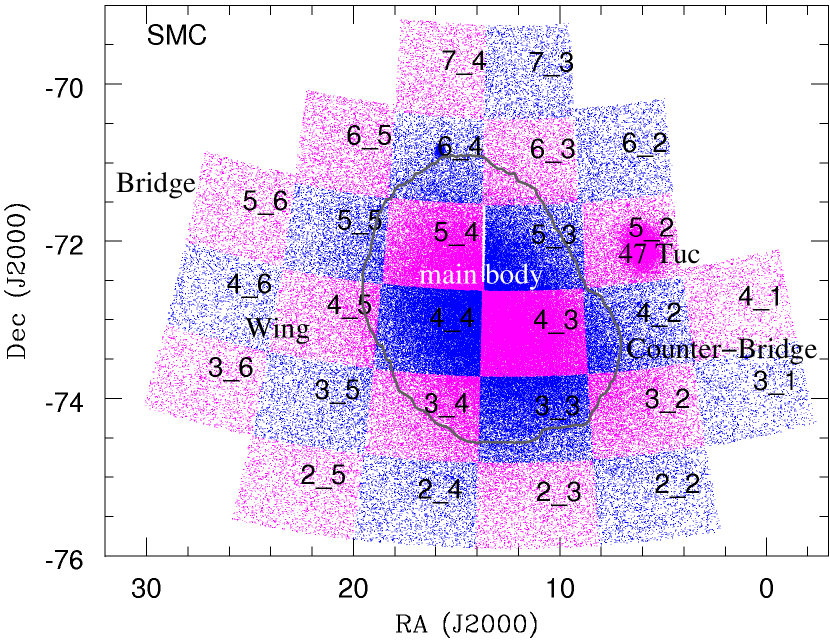
Figure 1: Map of sources with $K_{\rm s}=16$–$18$ mag from the VMC survey area around the SMC (the prominent dark area in the middle; the contour demarcates the boundary between ‘inner’ and ‘outer’ regions). The VMC tiles are labelled. The round overdensity seen at RA $=5\degr$, Dec $=-72\degr$ in tile SMC 5_2 is caused by the Galactic globular cluster 47 Tucanæ (another Galactic globular cluster, NGC 362, is visible in tile SMC 6_4 at RA $=16\degr$, Deg $=-71\degr$). The gap between tiles SMC 5_3 and SMC 5_4 (seen at RA $=13\hbox to0.0pt{.\hss}{\degr}5$) is caused by the absence of data.

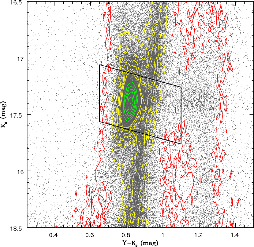
Figure 2: $K_{\rm s}$ versus $Y-K_{\rm s}$ diagram around the RC in tile SMC 5_3, showing the paralellogram selection box inclined along the reddening vector and limited at $(Y-K_{\rm s})=1.1$ mag to avoid Galactic foreground stars. The density contours are at 1% of peak (red), 5%–30% of peak with step 5% (yellow) and 50%–100% of peak with step 10% (green).

We used point spread function (PSF) fitted photometry (for full details see Rubele et al., 2012, 2015) instead of the aperture photometry that is provided by the VISTA Science Archive (VSA; Cross et al., 2012) as part of the VISTA pipeline products. Apart from improved performance in crowded regions, the PSF photometry was also found to be less susceptible to variations in seeing.

The tiles overlap by $\sim 10$ per cent. As the photometric catalogues were constructed on a tile-by-tile basis this means that some stars will have multiple entries in the catalogue. This is not a problem, as our analysis is not based on source counts. In fact it has the benefit that variations between tiles will be reduced in these overlapping regions, and that any dispersion in values introduced by multiple measurements is a measure of the accuracy with which these measurements had been derived.

3 Methods

3.1 RC selection

Each tile has its own RC star selection created using a two-dimensional histogram (Hess diagram) method, described by Tatton et al. (2013, Section 3.3). The only substantive difference with the procedures introduced by Tatton et al. (2013) is that they made use of the $J$ band instead of the $Y$ band. The reason is that, at the time, problems were noticed with the $Y$ band zero points that have meanwhile been resolved. With reliable $Y$-band photometry now available, the $Y$ band is preferred over the $J$ band, in conjunction with the $K_{\rm s}$ band, since the longer wavelength base helps determine – and correct for – the amount of reddening by interstellar dust, leading to more accurate reddening-corrected $K_{\rm s}$ values and thereby more accurate distance modulus estimates. Both the $Y$-band and $J$-band data are essentially complete for all RC stars; crowding and reddening lead to negligible losses.

Table 3: Tiles used and RC photometric properties. The columns list the tiles, their centres, the number of sources with magnitude readings in all three bands, the number of sources in the selected RC region followed by statistics on these RC regions: contour peak position (bin size 0.05 and 0.01 mag for $K_{\rm s}$ and $Y-K_{\rm s}$ respectively) and the $Y-K_{\rm s}$ mean, standard deviation (SD) and median values.

Tile	RAJ2000 ($\degr$)	DecJ2000 ($\degr$)	Sources		— Contour peak —		Mean	SD	Median
	°	°	Total	RC	$K_{\rm s}$ (mag)	–———— $Y-K_{\rm s}$ (mag) ————–
SMC 2_2	05.4330	$-$75.2012	84627	5486	17.45	0.82	0.822	0.065	0.810
SMC 2_3	11.1496	$-$75.3037	110576	10548	17.45	0.78	0.816	0.060	0.807
SMC 2_4	16.8911	$-$75.2666	137434	10941	17.50	0.80	0.906	0.179	0.830
SMC 2_5	22.5526	$-$75.0910	72423	5749	17.40	0.80	0.839	0.076	0.823
SMC 3_1	00.6663	$-$73.8922	76079	2068	17.40	0.75	0.792	0.075	0.780
SMC 3_2	05.8981	$-$74.1159	190401	18013	17.40	0.77	0.793	0.059	0.782
SMC 3_3	11.2329	$-$74.2117	1631078	56702	17.40	0.82	0.836	0.059	0.830
SMC 3_4	16.5880	$-$74.1774	288092	29794	17.40	0.83	0.840	0.058	0.834
SMC 3_5	21.8784	$-$74.0137	128290	7314	17.40	0.83	0.845	0.072	0.839
SMC 3_6	27.0255	$-$73.7245	97367	3542	17.40	0.78	0.818	0.074	0.803
SMC 4_1	01.3911	$-$72.8200	75399	1895	17.50	0.76	0.779	0.083	0.758
SMC 4_2	06.3087	$-$73.0299	245652	21829	17.45	0.78	0.809	0.070	0.794
SMC 4_3	11.3112	$-$73.1198	845029	125704	17.40	0.86	0.884	0.075	0.878
SMC 4_4	16.3303	$-$73.0876	693135	82330	17.40	0.86	0.872	0.075	0.868
SMC 4_5	21.2959	$-$72.9339	201070	11533	17.40	0.84	0.848	0.066	0.840
SMC 4_6	26.1438	$-$72.6624	70533	4310	17.00	0.81	0.828	0.069	0.815
SMC 5_2	06.6737	$-$71.9433	42860	3449	17.50	0.78	0.807	0.070	0.775
SMC 5_3	11.2043	$-$72.0267	2174210	45536	17.40	0.82	0.840	0.064	0.829
SMC 5_4	16.1088	$-$71.9975	536306	59231	17.35	0.84	0.858	0.069	0.849
SMC 5_5	20.7706	$-$71.8633	185805	14004	17.25	0.82	0.841	0.067	0.828
SMC 5_6	25.3700	$-$71.5964	93924	4151	17.00	0.77	0.799	0.068	0.782
SMC 6_2	06.9165	$-$70.8535	91744	3822	17.50	0.77	0.811	0.073	0.775
SMC 6_3	11.4532	$-$70.9356	123840	8814	17.50	0.79	0.830	0.061	0.817
SMC 6_4	15.9581	$-$70.8929	155280	12598	17.30	0.79	0.811	0.066	0.798
SMC 6_5	20.3437	$-$70.7697	118002	7433	17.00	0.77	0.796	0.066	0.781
SMC 7_3	11.5197	$-$69.8439	67270	3428	17.55	0.75	0.783	0.067	0.767
SMC 7_4	15.7520	$-$69.8162	77063	3632	17.50	0.78	0.798	0.066	0.783

To summarise, each tile has a RC selection box with a centre and size determined by the peak and width of the distribution of stars in the CMD and with a colour gradient determined by the reddening vector (Fig. 2). Contour plots are used to determine the centre and magnitude range within the box whereas histograms inside this box are used to determine the colour range. These values are summarised in Table 3. A “red” boundary to the selection box was imposed in order to avoid running into the vertical sequence of foreground stars (Fig. 2); owing to the metal-poor SMC stars being relatively blue, this was possible whereas in the LMC the two populations overlap (see Figure C.1 in Tatton et al., 2013). The foreground population appears to have an excess of stars only slightly brighter than the RC stars in Fig. 2. It is not clear what is the cause of this (they cannot be blended or reddened RC stars), but it does not affect our analysis.

In total 561,843 RC star candidates were found. The ‘inner’ and ‘outer’ SMC regions are defined by a density contour map of the SMC for the RC stars, where the outer SMC lies outside of the 20% contour level – this contains 161,100 sources.

Figure 3: CMDs for all tiles, each with their RC selection box and contour at 30% of the RC peak within the CMD.

3.2 Population effects

There are two possible population effects that could affect the assumptions made in the use of individual RC stars: intrinsic colour and brightness variations (or spread) resulting from age and/or metallicity variations (or spread), and contamination from stars that are not RC stars.

To start with the former, it is true that even in the K-band the RC brightness has the potential to vary by more than 0.5 mag, becoming brighter with younger age and higher metallicity (e.g., Figures 1 and 3 in Salaris & Girardi, 2002). This could lead to under-estimation of the distance modulus (or introduce an apparent foreground population) or – in the case of a mix of populations of a range in age and metallicity – an increased apparent depth. Because these population variations are largely due to bolometric correction variations the intrinsic colours will also change, which could lead to errors in the reddening determination and correction.

However, in reality the situation is not as extreme as one might envisage, because the SMC has been forming stars over many Gyr, gradually building up its metallicity. In combination with the mass-dependent stellar birth frequency and evolutionary timescales this results in a dominant age and metallicity corresponding to the assumed RC. Figure 13 in Rubele et al. (2018) proves this point: based on star formation and chemical evolution histories derived from the CMDs across the SMC, the RC stars effectively comprise intermediate age and only a narrow range in (typical SMC) metallicity, suggesting there is no cause for concern. In particular, there is no evidence for a significant contribution of (relatively) young RC stars. The RC does have a finite spread, even for a simple stellar population, but the core of the RC is very sharp ($\Delta K_{\rm s}\ll 0.1$ mag; Figure 6 in Rubele et al. (2018)) and comparable to the photometric spread. The spread derived from the inner two quartiles of the brightness distribution will measure mainly how much the core of the RC is spread, and be insensitive to intrinsic tails of the RC brightness distribution; while maps of the spatial distribution in the outer quartiles will show if and where there is an excess of stars that are brighter/fainter because they are nearer/farther.

As for the latter effect, contamination can arise principally from RGB stars and foreground stars. Figure 3 shows evidence for this, and how it may vary across the SMC. The contaminating foreground population comprises relatively cool, metal-rich stars in the Milky Way disc, seen along the red edge of the CMDs around $(Y-K_{\rm s})\approx 1.4$ mag. Here we are helped by the fact that SMC stars, even the RC stars, are relatively warm and metal-poor. This separates the two populations in colour, and given that the reddening is also relatively mild in the not very dusty metal-poor ISM of the SMC the two do not overlap. Nevertheless, the RC selection boxes are truncated at the red side so as to avoid the foreground, sacrificing the possible detection of rare highly-reddened RC stars – even in crowded fields with relatively dense, possibly dusty ISM such as SMC 4_3 there is no indication that such stars exist in abundance.

As is clear in Figure 3, however, the RGB within the SMC is crossed by the selection box. While the bulk of the RC is offset to bluer colours with respect to the bulk of the RGB, we had decided not to restrict the selection boxes further so as to avoid the RGB altogether, as this would introduce a stronger bias against reddened RC stars that could preferentially be at somewhat larger distances. Consequently, there is a fraction of the RC sample that are not in actual fact RC stars but RGB stars. The question is how this affects our analysis.

Firstly, as is clear from Figure 3, the RC is much more densely populated within the CMD than the RGB at similar brightness. The contours delineate 30% of the RC peak, and the RGB CMD density is well below that. Secondly, the RGB is populated much more uniformly in brightness, with a shallow and smooth gradient, in comparison to the RC (“branch” versus “clump”). This means that the RGB contamination should not lead to large deviations in the derived median distance modulus (as used in Section 5.3). It could have a larger effect on the apparent depth, but we mitigate against this by considering the brightness distribution of the RC stars excluding the tails of the distributions (see Section 5.4).

The largest effect could be on the derived RC reddening distributions. There is little reason to expect the spatial distribution in reddening (discussed in Section 4) to be affected substantially as the ratio of RC to RGB stars varies little across the SMC. However, we must look out for possible increases in stars that appear to be reddened significantly but that are actually (relatively) unreddened RGB stars. We discuss evidence for this, and quantify its effect, in Section 6.1.

3.3 Dereddening

It is possible to obtain a value for the $K_{\rm s}$ magnitude of an individual RC star free from extinction, based on its $Y-K_{\rm s}$ colour excess, $E(Y-K_{\rm s})$, with respect to its intrinsic colour, $(Y-K_{\rm s})_{0}$. A value of $(Y-K_{\rm s})_{0}=0.7625$ mag was determined from the average values using isochrones (Marigo et al., 2008; Girardi et al., 2010, converted to the VISTA photometric system by Rubele et al. 2012) that represent the SFH derived for the SMC from VMC PSF photometry by Rubele et al. (2015). In fact, the photometric properties of the bulk of the RC stars are not significantly affected by the effects of age or metallicity, especially in the near-IR (Alves, 2000; Onozato et al., 2019). This fiducial colour agrees very well with the observed blue end of the range of median values for the RC peak ($(Y-K_{\rm s})\approx 0.78$ mag; see Table 3); redder values indicate the effects of reddening.

The de-reddened magnitude can be expressed as:

$$(K_{\rm s})_{0}=K_{\rm s}-G\times\,E(Y-K_{\rm s}),$$ (1)

where $(K_{\rm s})_{0}$ is the resulting de-reddened magnitude and $G$ is the ratio of total to selective extinction (the ‘reddening vector’):

$$G=\frac{A_{K{\rm s}}/A_{V}}{A_{Y}/A_{V}-A_{K{\rm s}}/A_{V}}.$$ (2)

Using the $A_{\lambda}/A_{V}$ values for the VISTA filters (Tatton et al., 2013, their Table 2 based on the Cardelli et al. (1989) extinction law) we obtain $G=0.443$ and $A_{V}=3.69\times E(Y-K_{\rm s})$.

De-reddening is not carried out if $E(Y-K_{\rm s})<0$, which would have resulted from photometric scatter and intrinsic spread and not reddening. We do include these negative colour excess values in the reddening map so as not to bias it. We do also include those RC stars in the 3D structure analysis, without changes to their colours and magnitudes; a similar number of stars would be expected to the red of the RC fiducial colour, but all of those are treated as being reddened and their colours and magnitudes are corrected. The latter will introduce an offset in the distances estimated for these stars (bringing them nearer to us), but this is a small effect ($\Delta E(Y-K_{\rm s})\sim 0.03$ mag $\equiv 0.013$ mag), diluted by at least as many sources not affected, and systematic across the entire survey area.

4 Reddening map

Figure 4 shows the reddening map of the entire SMC on the $E(Y-K_{\rm s})$ scale along with the conversion to $A_{V}$, both on a star-by-star basis (left panel) and as mean values for the nearest 1000 RC stars (right panel). The latter results in a varying angular resolution, from $\sim 10^{\prime}$ in the densest parts of the SMC (175 pc at a distance of 60 kpc corresponding to the bulk of the SMC ) to $\sim 1^{\circ}$ in the outskirts (1.75 pc at a distance of 100 pc for a typical Galactic dust layer). Gonzalez et al. (2012) determined that 200 is an appropriate minimum number of RC stars over which to average based on the Gaussian distributions over $(J-K_{\rm s})$ colour of RC stars seen in the direction of the Galactic Bulge. The larger number of stars (1000) chosen here reflects the relatively low reddening in the direction of the SMC and larger distance of RC stars within the SMC, thus increasing the statistical errors and the stochastic width of the Gaussian distributions which, in turn, necessitates a larger number of sightlines to be combined. Both reddening maps are made available at the Centre de Données astronomiques de Strasbourg (CDS).

The field edges stand out more clearly than in Figure 1 as a result of the varying RC selection box (see Table 3). The streaks of missing data and occasionally high extinction in a North–South direction are due to the variable quantum efficiency of VISTA detector 16 . This is especially prevalent in tiles SMC 3_2 (centred at RA $=6\degr$, Dec $=-74\degr$) and SMC 5_4 (centred at RA $=16\degr$, Dec $=-72\degr$).

High extinction is mainly seen along the dense main body of the SMC, though it becomes more patchy towards north–western parts covered largely by tile SMC 5_3 (RA $\simeq 12\degr$, Dec $\simeq-72\degr$). The strongest features however are seen almost exclusively within tile SMC 4_3 (RA $=11\hbox to0.0pt{.\hss}{\degr}3$, Dec $=-73\hbox to0.0pt{.\hss}{\degr}1$). Evidently, the dust is concentrated in the main body where star formation is also most intense (e.g., Bolatto et al., 2011). In general for the whole SMC, lower extinction is seen in the Wing to the East of the main body.

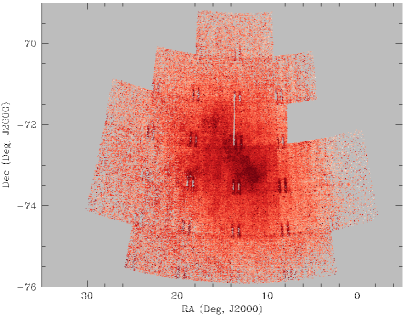
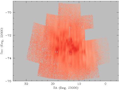
Figure 4: Reddening map of the SMC in $E(Y-K_{\rm s})$ (top side of legend shows this converted into $A_{V}$ magnitude) from RC stars. The vertical white strip around RA $=14\degr$ and Dec $=-72\degr$ lacks data, while the repeated pattern of pairs of short bars are caused by detector 16. The right panel shows the mean reddening values for the nearest 1000 RC stars.

5 Three-dimensional distribution of RC stars

5.1 Regional census

As a preliminary exploration of structure, the SMC RC star sample is divided into binned regions whose sizes vary with the stellar density. Owing to some SMC regions having very low stellar density this results in an incomplete coverage of the SMC, particularly within the Wing. Each cell in this regional census contains 500–2000 sources and has a size of 0.15–1 deg². This produces a total of 976 sub-regions, shown in Figure 5.

As expected, the median $(Y-K_{\rm s})$ colour follows the general pattern of the reddening map, where the inner SMC is redder than the outer regions. The representation in this figure, however, places more emphasis on high extinction regions – notably the area around RA $=18\hbox to0.0pt{.\hss}{\degr}5$, Dec $=-73\hbox to0.0pt{.\hss}{\degr}2$ associated with the N 83/84 star-formation complex.

From the de-reddened magnitudes (Figure 5, bottom right) it can be seen that the eastern Wing lies closer to us than the main body of the SMC, and the western periphery of the SMC is the furthest away. This appears to confirm the findings of Bica et al. (2015), who measured shorter distances to clusters within the Bridge (40–48 kpc). But the RC magnitude trend we see here is not a straightforward East–West gradient.

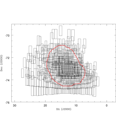
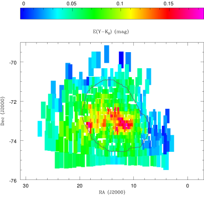
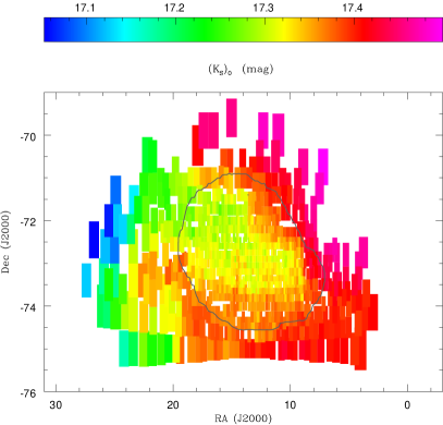
Figure 5: SMC maps of RC stars based on the regional census method. Shown are the outlines of the sub-regions (top–left), median $Y-K_{\rm s}$ colour (top–right), median $K_{\rm s}$ magnitudes before (bottom–left) and after (bottom–right) de-reddening. The contour represents the demarcation line between the inner and outer SMC fields.

5.2 SMC line-of-sight depth

There is a strong motivation to examine the line-of-sight depth in the SMC because it has been shown to have a thicker north–eastern side (e.g., Kapakos & Hatzidimitriou, 2012; Nidever et al., 2013; Subramanian et al., 2017).

Assuming that an RC star with $K_{\rm s}=17.304$ mag corresponds to a distance of 61 kpc (determined in the same way as the intrinsic colour in Section 3.3), we used the dispersion of distances in a binned region as a proxy for its thickness – i.e. line-of-sight depth.

For binned regions of $0\hbox to0.0pt{.\hss}{\degr}5$ in RA and $0\hbox to0.0pt{.\hss}{\degr}25$ in Dec, we look at this in two ways: first, the overall thickness range covered by all RC stars and, second, the thickness range of the two central quartiles of the distance distribution. While the former may over-estimate the line-of-sight depth due to contamination of the luminosity distribution by a ‘continuum’ of RGB stars, the latter likely under-estimates it since the RC luminosity distribution will have become truncated. Contour maps of these line-of-sight depth measures are shown in Figure 6.

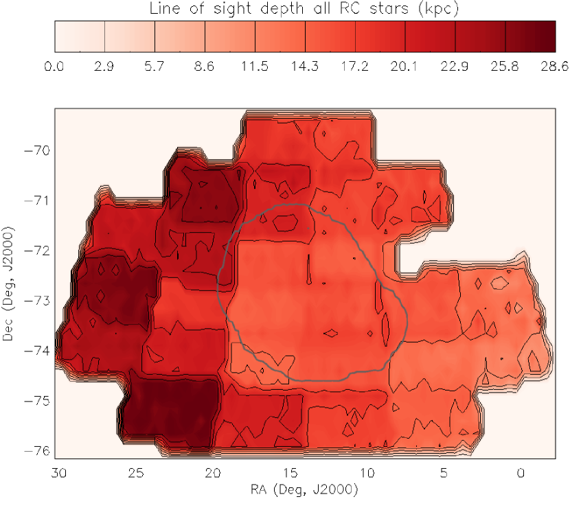
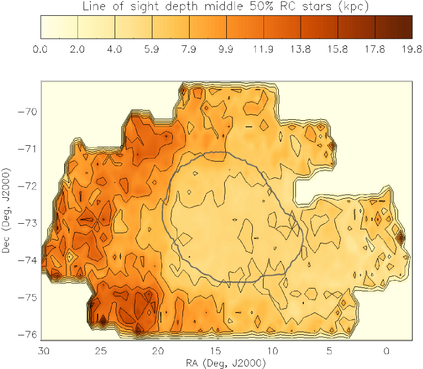
Figure 6: Line-of-sight depth of the SMC (in kpc) from RC stars, for all sources (top) and central quartiles (bottom). The bin size is $0\hbox to0.0pt{.\hss}{\degr}5$ in RA and $0\hbox to0.0pt{.\hss}{\degr}25$ in Dec.

The depth values themselves are typical of what is found in the literature, with central depths of $\sim 6$–14 kpc (Crowl et al., 2001; Subramanian & Subramaniam, 2012) and eastern depths of up to $\sim 23$ kpc towards the Bridge (Nidever et al., 2013).

When considering all sources one can see the effect of RC star selection and de-reddening having been conducted on a tile-by-tile basis, with the contour levels typically changing between tile edges. There is still significant line-of-sight depth exhibited in the central-quartiles sample. The major contributors to this depth are mostly the Wing regions in the North–East and South–East, but this is not a continuous band.

Another consideration is the distribution of distance moduli within the SMC. This analysis is carried out via histograms of the $K_{\rm s}$ magnitude for each tile and shown in Figure 7. It can be seen that for the eastern periphery (tiles SMC 2_5, SMC 3_6, SMC 4_6, SMC 5_6 and SMC 6_5) the distribution of sources does not only comprise a larger magnitude range than in the central and western regions but it also is double-peaked. This was first seen by Subramanian et al. (2017) in the North–East, but we now see that its presence is more wide-spread across the East. The fainter peak, at $K_{\rm s}\sim 17.3$–17.4 mag, corresponds to the bulk of the SMC. However, the brighter peak, at $K_{\rm s}\sim 16.9$–17.1 mag, corresponds to the distance to the LMC; it dominates over the fainter peak in tiles SMC 6_5, SMC 5_6 and SMC 4_6, which is in the direction of the LMC. Thus it is tempting to link this component to an effect caused by the LMC.

The north–western-most tiles (SMC 6_2 and SMC 4_1) have the dimmest peaks, around $K_{\rm s}\sim 17.5$ mag or $\sim 6$ kpc behind the SMC. It is possible that this is related to the Counter-Bridge (see Ripepi et al., 2017).

Figure 7: Histograms of de-reddened RC star $K_{\rm s}$ magnitudes (bin size of 0.02 mag for $K_{\rm s}=16.5$–18 mag range) for each SMC tile (labelled in the top–left or bottom–right of each panel). Of particular interest is the double RC seen in the eastern fields.

5.3 Plane fitting

We fit a plane to the spatial distribution of RC magnitudes, to examine whether a disc-like component is present in the SMC and to facilitate the examination of the structure by comparing the RC magnitudes relative to such a plane of symmetry. Moreover, to find the inclination and position angle (the orientation) of the SMC a plane must be fit. These values, apart from being of general interest when comparing with the orientation of the LMC and the path of motion through the Milky Way halo, may vary with the adopted tracer, thus revealing possible sub-structure and changes due to the dynamical history of the system.

In order to fit a plane to the data, we must remove the projection issues arising from the spherical co-ordinates that our current projection causes. This is done by transforming the current co-ordinate system of RA, Dec and measure of distance onto a Cartesian co-ordinate system where the $x$-axis is anti-parallel to RA, the $y$-axis is parallel to Dec and the $z$-axis points at the observer. The transformation takes the form of (e.g., van der Marel & Cioni, 2001; Subramanian & Subramaniam, 2010, 2013):

$$x=-D\times\sin(\,\alpha-\alpha_{0}\,)\times\cos\delta$$ (3)

$$y=D\times\sin\delta\times\cos\delta_{0}-D\times\sin\delta_{0}\times\cos(\,\alpha-\alpha_{0}\,)\times\cos\delta$$ (4)

$$z=D_{0}-D\times\sin\delta\times\sin\delta_{0}-D\times\cos(\,\alpha-\alpha_{0}\,)\times\cos\delta,$$ (5)

where ($\alpha_{0}$, $\delta_{0}$), ($\alpha$, $\delta$) and ($D_{0}$, $D$) are the RA, Dec and distance of the centre of the system and the sub-region, respectively.

A least-squares plane fitting procedure finds a solution to the following equation:

$$z=Ax+By+C.$$ (6)

The coefficients $A$, $B$ and $C$ are then used to obtain the position angle (PA) – of the line of nodes, i.e. the intersection of the galaxy plane with the plane of the sky, where it is measured from North over East (counter-clockwise) – and inclination ($i$) as follows:

$$i=\arccos\left(\frac{C}{\sqrt{A^{2}+B^{2}+1}}\right)$$ (7)

$${\rm PA}=\arctan\left(-\frac{A}{B}\right)+{\rm sign}(B)\times\frac{\pi}{2}$$ (8)

A single centre was used for the SMC which corresponds to the optical centre: RA $=13\hbox to0.0pt{.\hss}{\degr}17$, Dec $=-72\hbox to0.0pt{.\hss}{\degr}81$; this is an average of the values from de Vaucouleurs et al. (1976) and Paturel et al. (2003); see also de Grijs & Bono (2015). Plane fitting was carried out using all sources, outer sources (outside the 20% source density contour level), and the census method (see Section 5.1). The ‘all sources’, ‘outer ’ SMC and ‘census method’ samples contained 561,843 sources, 161,100 sources and 976 sub-regions, respectively. The results are summarised in Table 4.

Table 4: Plane fitting results to RC stars in the SMC.

	$i$ ($\degr$)	PA ($\degr$)
Outer	$48.5\pm 0.1$	$186.3\pm 0.5$
All	$43.3\pm 0.1$	$179.2\pm 0.1$
Census	$35.4\pm 1.8$	$169.8\pm 3.1$

The position angle from the ‘outer’ SMC fit returned a value of $-173\hbox to0.0pt{.\hss}{\degr}7$ but we use the complementary angle: $186\hbox to0.0pt{.\hss}{\degr}3$, following the adopted conventions of previous works. The cause of the rotation for the ‘outer’ fit result being reversed is most likely due to the centre of the Cartesian system being a void for that fit.

The census method acts as an inner SMC selection due to mainly containing sub-regions that are within the main body of the SMC. It is expected to exhibit a shallower inclination because the distribution over distance moduli is not sharply peaked in the core of the galaxy; also, the most extreme values are found outside of the main body of the SMC.

That said, the progressively larger inclination as well as rotation of the position angle, as one moves from the inner part of the SMC towards the periphery, could be an indication of tidal twisting of the SMC.

5.4 Deviations from a plane

For each selected RC candidate, the distance can be compared with the distance calculated at that position on the basis of the fitted plane solution. The difference between the two values is the ‘residual’. Figure 8 shows the histograms of these residuals for the three selections using a bin size of 0.2 kpc, where negative values lie behind the plane and positive ones lie in front of the plane.

One can see that the residual range of the two central quartiles is around 6 kpc (between boundaries ‘1’ and ‘3’), which is a good description of the line-of-sight depth for the central and western SMC depicted in Figure 6 (bottom panel). The central region, in particular, contains the majority of stars so this is not surprising. Examining the eastern SMC, line-of-sight depths are double this value. This was explained by their extended and split RC population as seen in Figure 7.

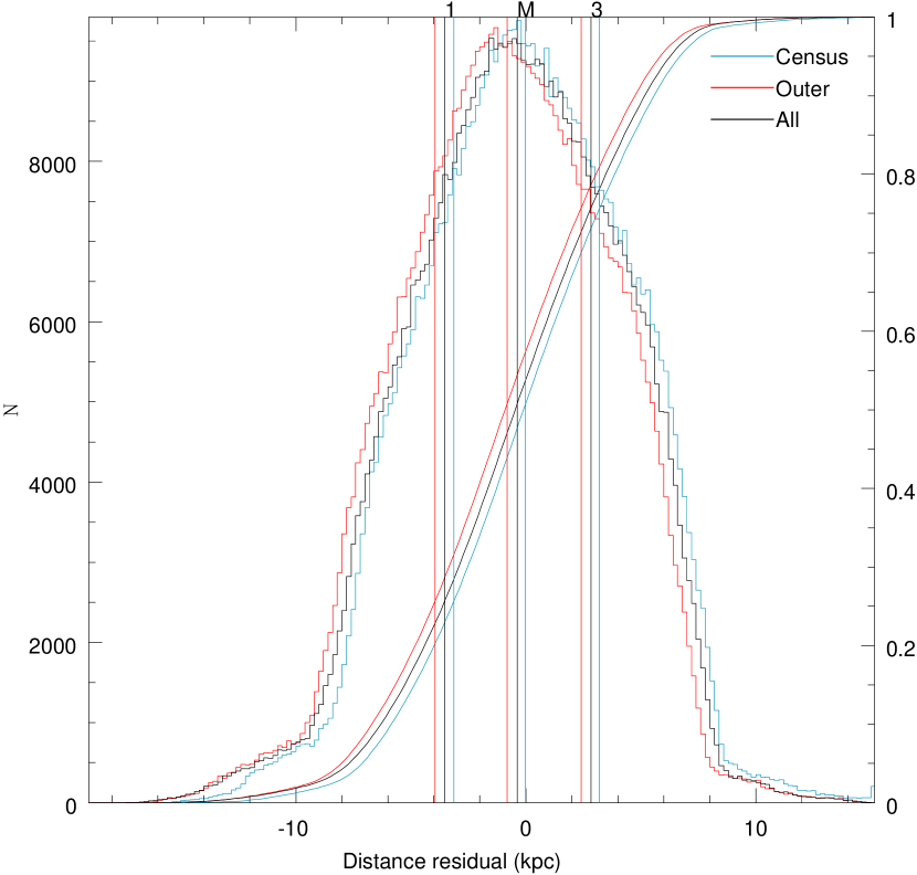
Figure 8: Histograms of residuals from the plane fits (bin size of 0.2 kpc) for ‘outer’ (red), ‘all’ (black) and ‘census’ (turquoise) SMC selections. The first (leftmost) and fourth (rightmost) quartiles cover a wide range of distances. Location of the boundaries between the quartiles are indicated with vertical lines and labelled as ‘1’, ‘M’ and ‘3’, respectively. Cumulative distributions are overlain (monotonically increasing curves, with values on the right hand side of the y-axis).

We split the residuals into four distance quartiles, from the back to the front of the plane, shown in Figure 9 for the ‘all’ SMC plane solution (the other two plane solutions are very similar). The bin size of these maps is $0\hbox to0.0pt{.\hss}{\degr}5$ in RA and $0\hbox to0.0pt{.\hss}{\degr}25$ in Dec. Displayed in these contour maps is the fraction of RC stars within a given bin contained in that quartile. For instance, high fractions in the second and third quartiles would suggest a compact structure commensurate with the plane fit, whereas high fractions in the first and fourth quartiles would suggest a highly extended or even split structure along the line-of-sight.

The main body of the SMC is found mostly in the latter three quartiles whereas its extent is small in the first (most distant) quartile. This would suggest that the main body of the SMC is a single component and not too extended in depth.

The eastern SMC (RA $>25\degr$) is mostly found in the first and last quartiles though, suggesting some asymmetry and distortion. The eastern tiles in general also exhibit greater line-of-sight depths (see Figure 6) and bimodal distance distributions (see Figure 7), which is reflected here in their presence in the first and fourth quartiles. Interestingly, in the first quartile there is less seen in the North–East but more in the South–East and this trend is reversed in the fourth quartile. With reference to Figure 7, most north–eastern tiles (e.g., SMC 5_6; RA $=25\hbox to0.0pt{.\hss}{\degr}4$, Dec $=-71\hbox to0.0pt{.\hss}{\degr}6$) have their largest peak of RC stars at relatively bright magnitudes, i.e. closer and thus in front of the plane of symmetry. The south–eastern tiles (e.g., SMC 3_5; RA $=21\hbox to0.0pt{.\hss}{\degr}9$, Dec $=-74\hbox to0.0pt{.\hss}{\degr}0$), on the other hand, contain relatively more fainter RC stars, which are farther and thus behind the plane of symmetry.

The northern part of the SMC (RA $=10\degr$–$20\degr$, Dec $>-71\degr$) is a more concentrated example of a single component appearing mainly in the first (far) quartile but non-existent in the fourth (near) quartile. In contrast the south–southeastern part (RA $=20\degr$–$26\degr$, Dec $<-75\degr$) is dominated by the near component.

The westernmost tiles (SMC 3_1 and SMC 4_1) are largely absent from the first quartile. This is confusing considering that the Counter-Bridge (see Ripepi et al., 2017) is a more distant feature and would be prominent behind the plane as opposed to in front. It is possible that so close to the main body of the SMC this distance increase has not yet manifested itself. Also, foreground contamination is relatively problematic in these sparse SMC fields.

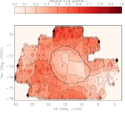
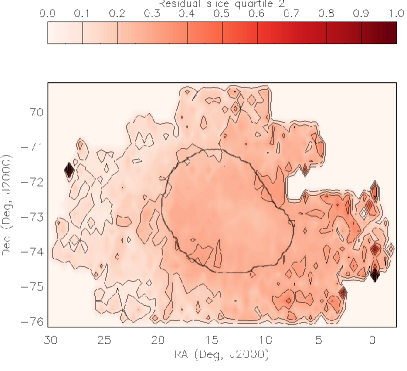
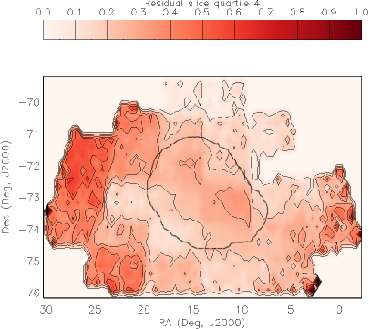
Figure 9: Residual slices with respect to a plane fitted to the ‘all’ SMC selection. Slices are ordered (clockwise) from behind the plane (first quartile, top–left) to in front of the plane (fourth quartile, bottom–right). Each slice contains 25% of the total number of RC stars; fractions, within bins of size $0\hbox to0.0pt{.\hss}{\degr}5$ in RA and $0\hbox to0.0pt{.\hss}{\degr}25$ in Dec, can be highly skewed across these distance slices.

6 Discussion

There are three main topics to discuss based on our new results: the reddening, the putative disc component and the morphological distortions.

6.1 Reddening (and dust)

While a comprehensive analysis of the reddening map similar to that in Tatton et al. (2013) is beyond te scope of the present study (cf. Bell et al., 2020), we will compare the spatial distributions of the interstellar dust and RC stars.

First, we compare our map with the widely used optical reddening map, expressed in $E(V-I)$, published by Haschke et al. (2011). We limited the comparison to their map based on RC stars (their Figure 4). Both maps contain some artificial structure – small gaps in ours and vertical striping in theirs. Qualitatively, the agreement is globally satisfactory, with peaks in similar places along the main body and also around N 83/84 in the Wing – though the latter seems more pronounced in their map. Our map covers a larger area on the sky, however, and clearly displays a smooth, ellipsoidal component with a reddening gradient away from the main body in all directions. This component is hard to discern in their map, apart from a global, low level of $E(V-I)\sim 0.04$ mag, corresponding to $A_{V}\sim 0.1$ mag, which seems to fall off at the extreme south–western and north–eastern edges of their map. Quantitatively, however, their reddening values correspond to $A_{V}$ values that are about three times lower than ours. A similar discrepancy had been noted for the 30 Doradus field in the LMC (Tatton et al., 2013), which was attributed to a combination of reddening bias and contamination from non-RC stars resulting from the more simplistic RC selection criteria adopted by Haschke et al. (2011). Górski et al. (2020) improved upon the work by Haschke et al.; their mean and maximum reddening values correspond to $A_{V}\sim 0.25$ and $\sim 0.70$, respectively, which match ours within a factor two.

Second, we compare our map with other ISM tracers. In the H$\alpha$ map of Kennicutt et al. (1995) the western side of the main body has similar emission levels to the south–eastern side. In the H i map of Stanimirović et al. (1999) and the mid- and far-IR maps of Bolatto et al. (2007) and Leroy et al. (2007), on the other hand, the western side of the main body has weaker emission than the eastern. The differences between the H$\alpha$ study and the other studies suggest there are changes in the ionisation state – and possibly the dust-to-gas ratio – between the western and eastern parts of the SMC main body. Dust emission is dependent on dust temperature and therefore the interstellar radiation field, whereas extinction is not. Thus, extinction is a more direct probe of dust.

In our extinction map weaker extinction is seen in the north–western side of the main body than in the South–East (see also Figure 5, top–right panel), corroborating what is seen in the H i and IR-emission maps and the reddening inferred using background galaxies (Bell et al., 2020). The strongest extinction features seen are best traced by the 8-$\mu$m data of Bolatto et al. (2007), suggesting that near-IR reddening may trace predominantly small grains (which are easily heated and thus shine brightly at relatively short IR wavelengths). The 160-$\mu$m data of Gordon et al. (2009) cover the Wing and main body and, unlike the previously mentioned maps, exhibit strands of emission connecting the main body with the Wing. In contrast, our map shows a more even distribution of moderate extinction between the two and strands are not apparent. This discrepancy can be explained by recalling the drawback of using extinction, which is that it is only measured in front of stars, whereas the dust emission is seen wherever it is located. Perhaps these strands of emission are predominantly located behind the stars resulting in less extinction measured than dust emission observed. Alternatively, if the strands are very thin, then few sightlines would cross them.

Another interpretation of our data comes from looking at the $Y-K_{\rm s}$ colours for the regional census sub-regions (Figure 10). A trend can be seen of average extinction increasing with respect to source density (i.e. the inner SMC has higher extinction than the outer SMC). This means that, to some extent, stars and dust are well mixed and follow the same potential. The scatter around this correlation is probably intrinsic, and the fact that the densest regions are not located where the colours reach the reddest values probably traces the recent star formation occurring in stripped gas devoid of an old stellar population. A particular high-extinction feature can be seen in the census map (Figure 5, top–right panel) around RA $=18\hbox to0.0pt{.\hss}{\degr}5$, Dec $=-73\hbox to0.0pt{.\hss}{\degr}3$. This is associated with the molecular cloud complex N 83/84.

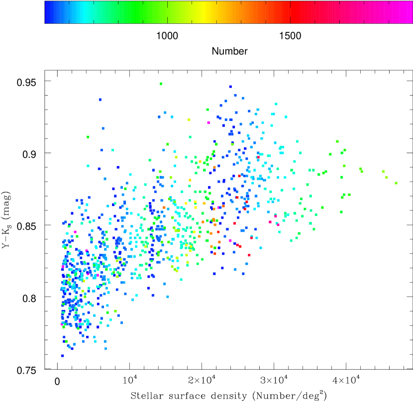
Figure 10: $Y-K_{\rm s}$ colour vs. regional census sub-region density of RC stars, showing a positive correlation (albeit with considerable scatter). The colour scale quantifies the number of sources per sub-region.

Finally, we examine the extinction distribution of five Wing tiles (SMC 2_5, SMC 3_6, SMC 4_6, SMC 5_6 and SMC 6_5) by splitting their populations into a near component ($K_{\rm s}<17.2$ mag, 12,855 RC stars) and a far component ($K_{\rm s}>17.2$ mag, 12,339 RC stars). The resulting histogram is shown in Figure 11. We might have expected more distant stars to experience higher extinction than stars in front, yet this is not seen. The overall distributions are in fact very similar, and no systematic shift is discernible. A feature that stands out more clearly is an excess of nearer stars apparently experiencing $A_{V}\sim 0.5$–0.8 mag. This can be traced back to the RGB bump, in Fig. 2 at $K_{\rm s}\approx 17.0$ mag and $(Y-K_{\rm s})\approx 0.95$ mag, and is seen in all tiles (see Section 3.2 for a discussion of population effects). The far component is fainter than the RGB bump, so is not affected by it, but the RGB itself still leaves an imprint. As Fig. 2 shows, this part of the RGB is less populated than the RGB bump, closer to the RC but bent more and thus the effect is both weaker and more wide-spread over $A_{V}$ – and therefore only appears as an inconspicuous shoulder to the extinction distribution around $A_{V}\sim 0.4$ mag. The reddening map is not dramatically affected by this inherent feature of the methodology, but it is important to be aware of its existence when using the map in all its fine detail.

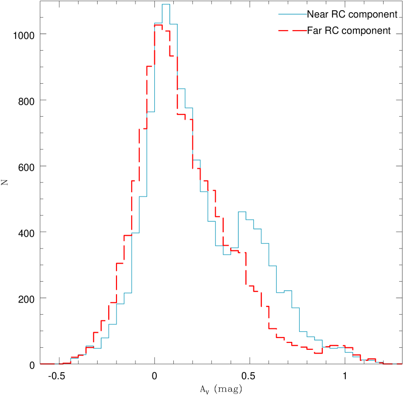
Figure 11: Histogram (bin size of 0.04 mag) comparing the extinction distribution of RC stars in the near-Wing component (turquoise, solid) to that in the far-Wing component (red, dashed).

6.2 Disc component

The inclination and position angle values found in the literature (see Table 2) greatly vary depending on the adopted tracer and method. This makes a direct comparison tricky, but potentially insightful. Younger Cepheid populations tend to have very steep inclinations – even though they do not strictly speaking adhere to a flat disc geometry (Ripepi et al., 2017, their Fig. 17). Older populations, on the other hand, tend to have very shallow, almost non-existent inclination – the oldest populations are more likely to be more spheroidal, as in the Milky Way halo, rather than being represented by a disc-like structure. One would therefore expect intermediate-aged populations traced, for instance, by RC stars to be somewhere between those. This is exactly what we found.

Subramanian & Subramaniam (2012) also used RC stars but found a very small inclination, $i=0\hbox to0.0pt{.\hss}{\degr}5$. Their methodology however was to use axes ratios and to limit the sample to a small depth range, which may have inadvertently introduced a bias. The position angles we found are nearest to those determined by Subramanian & Subramaniam (2015), who used Cepheids, and Rubele et al. (2015), who fitted entire CMDs and found a mean $i=39\degr$.

In conclusion, while the SMC does not exhibit an obvious disc component there is a clear trend for the system to become more inclined with respect to the plane of the sky the younger the (stellar) tracer is. Since the RC stars already show this progression this means that the dynamical events that led to this time-dependent morphology must have occurred on Gyr timescales. Indeed, while most of the stellar mass in the SMC was generated $>4$ Gyr ago (Sabbi et al., 2009; Rezaeikh et al., 2014; Rubele et al., 2018) there is evidence in the SFH of the SMC of a strong interaction with the LMC to have occurred $\sim 2$ Gyr ago (Harris & Zaritsky, 2004; Noël et al., 2009; Rezaeikh et al., 2014; Rubele et al., 2015). A more recent interaction $\sim 0.2$ Gyr ago coincident with the closest approach to the Milky Way, also seen in the SFH (Harris & Zaritsky, 2004; Noël et al., 2009; Sabbi et al., 2009; Rubele et al., 2015), may have caused further distortion of the gaseous disc, from which the younger population traced by the Cepheids formed.

6.3 Distortions and other structures

The outer regions of the SMC have been transformed by interactions leading to stripping and spatially stretched populations. Dias et al. (2016) described the SMC as being composed of three bodies: the eastern Wing, the central main body, and the western halo. We find the intermediate-age main body traced by RC stars to be structurally simple and symmetrical, consistent with a spheroidal component. The eastern Wing, on the other hand, is split into two distinct populations (both traced by intermediate-age RC stars), of which the brighter one clearly lies in front of the main body (Fig. 9, bottom–right). We have been able to comprehensively trace these two components across the VMC footprint, allowing us to relate them to what other observational and theoretical studies have found. We find a fourth structure, in the North (Fig. 9 top–left); this has previously been described as an extension to the Wing (e.g., Gardiner & Hawkins, 1991), but Sun et al. (2018) showed this area to contain a shell of young stars which is clearly separated from the general Wing area. The intermediate-age population of RC stars in the North need not be related to these young stars, though. We compare our results with previous analyses of Cepheids, RR Lyræ and RC stars, in light of these structures.

Ripepi et al. (2017) showed that both the young and old Cepheids (old Cepheids are $\sim 300$ Myr old, i.e. still much younger than RC stars) populate off-centre structures in the direction of the LMC. Nidever et al. (2013) found that the eastern side of the SMC has a bimodal distribution with a near component at 55 kpc and a far component at 67 kpc. In the same eastern regions we see a large line-of-sight depth but the sources are located mainly in front of the plane (i.e. a near component). However, these features may not be representative of the full content of the entire Wing. Young structures such as NGC 602 (RA $=22\degr$, Dec $=-73\hbox to0.0pt{.\hss}{\degr}6$) and N 83/84 (RA $=18\hbox to0.0pt{.\hss}{\degr}5$, Dec $=-73\hbox to0.0pt{.\hss}{\degr}2$) trace sub-structure not seen in the intermediate-age populations. Hammer et al. (2015) showed that past interactions between the LMC and SMC may have resulted in multiple tidal and ram-pressure stripped structures; while tidal effects are largely non-discriminatory in age, ram pressure can spatially separate gas in which new stars may form, from pre-existing (i.e. older) stellar populations.

Subramanian & Subramaniam (2012) selected optical photometry of RC stars and RR Lyræ (which are older than RC stars by a factor of a few, viz. $>10$ Gyr) and found typical line-of-sight depths of $4.6\pm 1.0$ kpc which increased to 6–8 kpc in the North–East. Muraveva et al. (2018) used VMC photometry of RR Lyræ and found an ellipsoidal distribution. Line-of-sight depths were in the range of 1.5–10 kpc, with an average of $4.4\pm 1.0$ kpc; these are around a factor of two smaller than the values derived here for RC stars (for the central quartiles we see a range of 0.5–20 kpc with an average of 7.8 kpc). We confirm the larger line-of-sight depth in the North–East; an increased depth in the South–West is less obvious and easier to see in the full line-of-sight depth map (Fig. 6).

Using a limited VMC data set, Subramanian et al. (2017) found a double RC feature manifesting itself as a distance bimodality in the eastern SMC with a ‘foreground’ population $\sim 11$ kpc nearer to us than the main SMC body. We confirmed this bimodality (see Figure 7) and showed it is also seen within adjacent tiles not studied by Subramanian et al. (2017): tiles SMC 2_5 (RA $=22\hbox to0.0pt{.\hss}{\degr}5$, Dec $=-75\hbox to0.0pt{.\hss}{\degr}1$), SMC 4_6 and SMC 3_6 (RA $=27\degr$, Dec $=-72\degr$ to $-74\degr$). The extent of the RC bimodality has since been traced further by El Youssoufi et al. (submitted). In addition, the northern tile SMC 7_4 (RA $=15\hbox to0.0pt{.\hss}{\degr}8$, Dec $=-69\hbox to0.0pt{.\hss}{\degr}9$) also exhibits some bimodality but spanning a less extended magnitude range. The closer of the two components is found around $K_{\rm s}\simeq 17.0$ mag making it much nearer to the LMC ($K_{\rm s}\simeq 16.9$ mag) than to the SMC ($K_{\rm s}\simeq 17.4$ mag).

The RR Lyræ do not show a distance bimodality (Muraveva et al., 2018) – while the eastern part of the SMC seems tilted towards us (their figure 15), there is a distinct lack of RR Lyræ $\sim 0.5$ mag brighter than those in the main body of the SMC (see their figure 8). This might suggest that the nearer RC component resulted from ram-pressure stripping of gas a few Gyr ago which led to subsequent formation of stars including what are now RC stars and Cepheids but without the presence of older stars such as RR Lyræ. A tidal origin would have affected stars of all ages similarly. This could mean that the Wing is, in origin, an intermediate-age structure that has persisted for a few Gyr; more recent tidal interactions could have shaped it further still.

An origin for the Bridge and the nearer RC component, and possibly the Wing, much earlier than a few hundred Myr is also consistent with the lower metallicity in the gas from which younger stars have formed in western parts of the Bridge (Rolleston et al., 1999; Lehner et al., 2008; Gordon et al., 2009). If these structures had formed from the main body of the SMC only a few hundred Myr ago then their metallicity ought to be indistinguishable from that of the ISM and young stars within the main SMC body. However, the metallicity in the Wing is much more similar to that within the main SMC body (Lee et al., 2005). This may be explained if, since the initial dislodging from the main body a few Gyr ago, star formation and chemical evolution within the eastern elongated structures continued on a par with that in the main body of the SMC in the densest parts closest to the SMC (Wing), whilst it proceeded much more slowly in the more tenuous parts further away (Bridge). Direct determination of the metallicity of the nearer RC stars could establish the connection between this intermediate-age component and the younger stars in the Wing, or the older stars in the Bridge.

While recent hydrodynamical simulations by Wang et al. (2019) show the separation of gas and stars due to the differing effects from tidal disruption and ram pressure interaction, they fail to reproduce the split RC and in particular the location on the sky of the far component. It is possible that this is a function of the exact (pre-)collision characteristics $>200$ Myr ago.

It is not just the East that is expected to display a distorted morphology. A Counter-Bridge originating in the West is predicted by the models of Diaz & Bekki (2012) as a remnant of the last close LMC–SMC encounter. However, due to the distances involved (70–80 kpc) its existence has so far only been suggested by Ripepi et al. (2017) and Niederhofer et al. (2018). We may be seeing a somewhat more distant RC clump in the far West (Fig. 7, tile SMC 4_1), though we caution that the source density is low. However, the Counter-Bridge is predicted to wrap around the SMC, from the South–West to the North–East. The dominance of ‘distant’ RC stars in the North (Fig. 9, top–left) could plausibly be associated with that part of the Counter-Bridge. Our finding is corroborated by El Youssoufi et al. (submitted). In fact, the foreground component appears to cross the main body of the SMC from North–East to South–West (Fig. 9, bottom–right); while this is dependent on the location of the ‘plane’ that was fit, the absence of a background component at the location of the main body of the SMC seems to confirm this interpretation. This suggests that both the Wing/Bridge and Counter-Bridge may have been stripped from the SMC first, trailing the SMC in its wake, before having been stretched by tidal effects.

7 Conclusions

This work used near-IR survey data of the SMC from the recently completed VMC survey, and reliable, homogenised PSF photometry covering the entire galaxy, to map its structure as traced by intermediate-age RC stars in unprecedented detail. The near-IR has the advantage that the effects from interstellar reddening and population age and metallicity are much reduced compared with the optical. That said, we did derive also a reddening map, which showed general agreement with dust emission and which was used to correct the $K_{\rm s}$-band magnitudes of the RC stars.

The large line-of-sight depths seen in the East led us to re-examine the magnitude distributions of the RC stars across the SMC. From this, a double RC component was seen whose nearer component is around the LMC distance. While this feature had been reported in Subramanian et al. (2017), here we expanded upon that study by showing how this feature varies across a larger area of the sky.

The residuals from fitting a plane once again emphasised that these eastern regions reveal structure that is not described by a plane in the periphery of the SMC. The inclination derived from plane fitting solutions ($i=35\hbox to0.0pt{.\hss}^{\circ}4\pm 1\hbox to0.0pt{.\hss}^{\circ}8$ for the inner-dominated census selection) falls between the very shallow inclinations reported for older RR Lyræ populations ($i\simeq 2\degr$) and younger Cepheid populations ($i\simeq 60\degr$). A distant population of RC stars seen in the North may be associated with the Counter-Bridge, as predicted by tidal interaction models.

The structures within the SMC mainly arise from its past close interactions with the LMC, which is evident in the sense that the East – which is nearest to the LMC – has the greatest distortions. The fact that some of these structures are traced by RC stars but not RR Lyræ stars means that tidal effects cannot fully account for them and star formation a few Gyr ago in ram-pressure stripped gas must be invoked.

Data Availability

The photometry data used in this paper are available in the VISTA Science Archive (VSA), at http://horus.roe.ac.uk/vsa
The reddening map catalogues derived from this data (presented in Figure 4) will be available in Centre de Donnees astronomiques de Strasbourg (CDS), at https://cds.u-strasbg.fr

References

- Alves (2000) Alves D. R., 2000, ApJ, 539, 732
- Bekki & Chiba (2008) Bekki K., Chiba M., 2008, ApJ, 679, L89
- Bell et al. (2020) Bell C. P. M., et al., 2020, MNRAS,
- Belokurov & Erkal (2019) Belokurov V. A., Erkal D., 2019, MNRAS, 482, L9
- Belokurov et al. (2017) Belokurov V., Erkal D., Deason A. J., Koposov S. E., De Angeli F., Evans D. W., Fraternali F., Mackey D., 2017, MNRAS, 466, 4711
- Besla et al. (2016) Besla G., Martínez-Delgado D., van der Marel R. P., Beletsky Y., Seibert M., Schlafly E. F., Grebel E. K., Neyer F., 2016, ApJ, 825, 20
- Bica et al. (2015) Bica E., Santiago B., Bonatto C., Garcia-Dias R., Kerber L., Dias B., Barbuy B., Balbinot E., 2015, MNRAS, 453, 3190
- Bolatto et al. (2007) Bolatto A. D., et al., 2007, ApJ, 655, 212
- Bolatto et al. (2011) Bolatto A. D., et al., 2011, ApJ, 741, 12