A Three-Point Form Factor Through Five Loops

Abstract

We bootstrap the three-point form factor of the chiral part of the stress-tensor supermultiplet in planar $\mathcal{N}=4$ super-Yang-Mills theory, obtaining new results at three, four, and five loops. Our construction employs known conditions on the first, second, and final entries of the symbol, combined with new multiple-final-entry conditions, “extended-Steinmann-like” conditions, and near-collinear data from the recently-developed form factor operator product expansion. Our results are expected to give the maximally transcendental parts of the $gg\to Hg$ and $H\to ggg$ amplitudes in the heavy-top limit of QCD. At two loops, the extended-Steinmann-like space of functions we describe contains all transcendental functions required for four-point amplitudes with one massive and three massless external legs, and all massless internal lines, including processes such as $gg\to Hg$ and $\gamma^{*}\to q\bar{q}g$. We expect the extended-Steinmann-like space to contain these amplitudes at higher loops as well, although not to arbitrarily high loop order. We present evidence that the planar $\mathcal{N}=4$ three-point form factor can be placed in an even smaller space of functions, with no independent $\zeta$ values at weights two and three.

feyndiags

1 Introduction

The most important production mechanism for the Higgs boson at the Large Hadron Collider is the gluon fusion process, mediated by a top quark loop. Higher-order QCD corrections to this process are very large, necessitating its understanding to at least next-to-next-to-next-to-leading order (N³LO) in the strong coupling $\alpha_{s}$ Anastasiou:2015vya ; Mistlberger:2018etf . In particular, matrix elements for the Higgs boson plus $n$ additional gluons are required. In the limit where the mass of the top quark is taken to be infinite, these amplitudes can be thought of as the $n$-point form factors of the gauge-invariant local composite operator $\operatorname{tr}(F^{2})$ Wilczek:1977zn ; Shifman:1978zn :

$$\mathcal{F}_{\operatorname{tr}(F^{2})}(p_{1},\dots,p_{n};q)=\int d^{d}x\,e^{-iq\cdot x}\langle 1,\dots,n|\operatorname{tr}(F^{2})(x)|0\rangle\,,$$ (1)

where $p_{i}$ denotes the momentum of the $i^{\text{th}}$ external particle, and $q$ is the momentum of the operator insertion, or equivalently the momentum of the Higgs boson.

At tree level, the operator $\operatorname{tr}(F^{2})$ can be split into a self-dual part $\operatorname{tr}(F_{SD}^{2})$ and an anti-self-dual part $\operatorname{tr}(F_{ASD}^{2})$, exposing a helicity structure similar to that for pure-gluon amplitudes Dixon:2004za . At loop level, when the form factor is normalized by its tree-level value, the kinematic dependence is trivial for $n=2$ (where it corresponds to the Sudakov form factor), and becomes non-trivial for $n\geq 3$. The three-point form factor $\mathcal{F}_{\operatorname{tr}(F^{2})}$ in QCD is currently known up to two loops Gehrmann:2011aa , which is the order contributing to the N³LO terms in the Higgs production cross section. Curiously, the maximally transcendental part of this form factor, or more specifically of its remainder function Bern:2008ap ; Drummond:2008aq , has been shown to coincide with its counterpart in the maximally supersymmetric Yang-Mills ($\mathcal{N}=4$ sYM) theory Brandhuber:2012vm , where $\operatorname{tr}(F_{SD}^{2})$ is part of the larger chiral part of the stress-tensor supermultiplet. This finding is an example of the more general principle of maximal transcendentality Kotikov:2001sc ; Kotikov:2002ab ; Kotikov:2004er ; Kotikov:2007cy , which relates the results for many interesting quantities in $\mathcal{N}=4$ sYM theory to the maximally transcendental part of their counterparts in pure Yang-Mills theory.

Form factors of a variety of operators have been calculated in $\mathcal{N}=4$ sYM theory using modern techniques originally developed in the context of scattering amplitudes. These include recursion relations Brandhuber:2010ad ; Brandhuber:2011tv ; Bolshov:2018eos ; Bianchi:2018peu , on-shell diagrams, polytopes and Graßmannians Bork:2014eqa ; Bork:2015fla ; Frassek:2015rka ; Bork:2016hst ; Bork:2016xfn ; Bork:2017qyh , twistor space actions Koster:2016ebi ; Koster:2016loo ; Chicherin:2016qsf ; Koster:2016fna , a connected prescription He:2016dol ; Brandhuber:2016xue ; He:2016jdg , color-kinematics duality Boels:2012ew ; Yang:2016ear ; Lin:2020dyj , and a dual description via the AdS/CFT correspondence Alday:2007he ; Maldacena:2010kp ; Brandhuber:2010ad ; Gao:2013dza ; Ben-Israel:2018ckc ; Bianchi:2018rrj . These results are currently limited to two loops for $n\geq 3$. See ref. Yang:2019vag for a recent review.

Prominent among these modern techniques are bootstrap methods Dixon:2011pw ; Dixon:2013eka ; Caron-Huot:2016owq , which have been used in planar $\mathcal{N}=4$ sYM theory to determine the six-point amplitude through seven loops Caron-Huot:2019vjl and the seven-point amplitude through four loops Drummond:2014ffa ; Dixon:2016nkn ; Drummond:2018caf ; Dixon:2020cnr . They have also been used to verify Almelid:2017qju the three-loop soft anomalous dimension matrix Almelid:2015jia , which contributes to the infrared structure of gauge theory beyond the planar limit. Bootstrap methods are based on making an ansatz for the functional form of the amplitude, leveraging knowledge of the location of its possible discontinuities, as well as conditions on its derivatives and higher discontinuities. Coefficients in the ansatz are fixed by requiring it to have appropriate discrete symmetries and by matching it to various physical limits.

One important set of constraints for these bootstrap methods comes from the behavior of these amplitudes in near-collinear limits. Their expansion around this limit is described at all loop orders by the integrability-based pentagon operator product expansion (POPE) Basso:2013vsa ; Basso:2013aha ; Basso:2014koa ; Basso:2014nra ; Basso:2014hfa ; Basso:2015rta ; Basso:2015uxa ; Belitsky:2014sla ; Belitsky:2014lta ; Belitsky:2016vyq . Recently, an analogous description of the near-collinear limit of form factors has been developed, termed the form factor operator product expansion (FFOPE) Sever:2020jjx ; Toappear1 ; Toappear2 . It provides physical constraints on the near-collinear behavior of the form factors of the chiral part of the stress-tensor supermultiplet at any loop order.

In this paper, we study the three-point maximum-helicity-violating (MHV) form factor of the chiral part of the stress-tensor supermultiplet. This form factor depends on the three ratios $u=s_{12}/q^{2}$, $v=s_{23}/q^{2}$ and $w=s_{31}/q^{2}$. However, since $q^{2}=s_{123}=s_{12}+s_{23}+s_{31}$, these variables satisfy the constraint $u+v+w=1$, and the form factor actually depends on only two variables. These are exactly the same variables on which the corresponding Higgs boson amplitudes in QCD depend. The two-loop contribution to this form factor has been computed via unitarity methods; moreover, it was shown to be uniquely determined by a bootstrap approach involving conditions on the first, second, and final entries of the symbol Brandhuber:2012vm . The first two entry conditions restrict the single and double discontinuities of the form factor, while the final-entry conditions constrain its differential structure. Here we exploit the recent progress on the FFOPE to bootstrap this form factor all the way to five loops.

In addition to leveraging the FFOPE, we observe and exploit two new forms of mathematical structure in the infrared-finite part of the form factor, which are not obeyed by the remainder function. First, we observe new multiple-final-entry conditions that restrict linear combinations of the last two or three entries of the symbol of the form factor. Second, we discover certain “extended-Steinmann-like” (ES-like) conditions Caron-Huot:2019bsq ; Drummond:2017ssj at all depths in the symbol. In the three-point form factor alphabet $\{u,v,w,1-u,1-v,1-w\}$, these ES-like conditions imply that $1-u$ never appears next to $1-v$ or $1-w$ in the symbol, nor $1-v$ next to $1-w$. While this condition does not transparently follow from the standard Steinmann relations, it is inspired by studying the Steinmann and cluster algebra constraints for heptagon functions Dixon:2016nkn ; Drummond:2017ssj , since the pentabox ladder integrals Drummond:2010cz ; Caron-Huot:2018dsv contribute to both the seven-particle amplitude and the three-point form factor.

To carry out our bootstrap, we define a space of polylogarithmic functions $\mathcal{M}$ that contains the infrared-finite part of the form factor. This function space draws from the symbol alphabet $\{u,v,w,1-u,1-v,1-w\}$ and obeys the ES-like conditions described in the last paragraph. We find that the dimension of $\mathcal{M}$ is exactly $3^{w}$ at weight $w$ (at symbol level). Although this growth rate is considerably slower than without the ES-like conditions, it is still considerably faster than the hexagon function space ${\cal H}$ associated with the six-point amplitude, which grows approximately as $\sim 1.8^{w}$ Caron-Huot:2019bsq . On the other hand, the simple dependence of the dimension on the weight suggests that a direct construction of this function space should be possible.

In the absence of a direct construction of $\mathcal{M}$, it would be helpful if there were a smaller space of functions that contained the finite part of the form factor. And indeed, when we normalize the form factor in a slightly different way, we learn by taking its derivatives (or rather, its iterated $\{n-1,1\}$ coproducts) that the space $\mathcal{M}$ is still larger than necessary for the planar ${\cal N}=4$ form factor. We also begin to see aspects of cosmic Galois theory, or the coaction principle Schnetz:2013hqa ; Brown:2015fyf ; Panzer:2016snt ; Schnetz:2017bko , which is also seen in the space of hexagon functions Caron-Huot:2019bsq . Notably, in this smaller space $\mathcal{C}$, the constants $\zeta_{2}$ and $\zeta_{3}$ no longer need to be treated as independent functions; they are locked to the other, symbol-level functions.

The rest of this paper is structured as follows. We review some basic properties of the three-point MHV form factor of the chiral part of the stress tensor in section 2. Moreover, we analyze its two-loop remainder function, which exhibits many of the properties that we will generalize to higher loop orders in subsequent sections. In section 3, we construct the function space $\mathcal{M}$ in which the form factor lives. We then bootstrap this form factor at three-, four-, and five-loop orders, and analyze the minimal space $\mathcal{C}\subset\mathcal{M}$ that appears in the coproduct of these functions in section 4. In section 5, we study the behavior of the remainder function through five loops, plotting its dependence on various combinations of parameters, and considering several kinematic limits. In section 6, we present evidence that the space $\mathcal{M}$ may also govern amplitudes with the same kinematics in arbitrary massless theories. Our conclusions and outlook are contained in section 7.

There are two appendices. Appendix A describes the pentabox ladders and their relation to both $\mathcal{M}$ and heptagon functions. Appendix B collects some explicit results for the near-collinear limits of the form factor remainder function needed to make contact with the FFOPE.

Ancillary files: We include three ancillary files. The first one, cEandRsymbols.txt, gives the symbols of the finite part of the form factor through five loops, and of the remainder function through four loops. The second and third files, T2terms.txt and T4terms.txt, provide the $T^{2}$ and $T^{4}$ terms, respectively, in the near-collinear limit through five loops.

2 BPS Form Factors and Polylogarithms

In this paper, we study the half-BPS operator corresponding to the chiral part of the stress-tensor supermultiplet in planar $\mathcal{N}=4$ sYM theory. This supermultiplet includes the scalar operator $\operatorname{tr}(\phi^{2})$, which is part of the so-called $20^{\prime}$ multiplet, as well as the chiral part of the on-shell Lagrangian, which includes the self-dual operator $\operatorname{tr}(F_{SD}^{2})$. We refer to refs. Eden:2011yp ; Brandhuber:2011tv ; Bork:2014eqa for more background on these form factors, and their formulation in $\mathcal{N}=4$ harmonic superspace.

Similar to scattering amplitudes, a helicity degree can be assigned to form factors, corresponding to the helicity of the $n$ external massless states. Form factors with helicity degree $n-k-2$ are related to those with helicity degree $k$ by parity, which acts on the external states as well as on the operator. Thus, non-trivial N^kMHV form factors first occur for $n=2k+2$.

For $n=2$ external states, the form factor only depends on the single scale $s_{12}=(p_{1}+p_{2})^{2}$, where $p_{i}$ is the momentum associated with the $i^{\text{th}}$ external state. Dimensional analysis dictates that this scale dependence has to factor out, leaving us with just a number at each perturbative order. The first case described by a non-trivial function thus involves $n=3$ external states. The only non-trivial form factor for this number of external states is MHV, namely $\mathcal{F}_{n,k=0}\equiv\mathcal{F}_{n}^{\rm MHV}$.

The form factor $\mathcal{F}_{3}^{\rm MHV}$ is a function of the three Mandelstam variables $s_{12}$, $s_{23}$, $s_{31}$ with

$$s_{ij}=(p_{i}+p_{j})^{2}=2p_{i}\cdot p_{j}\,.$$ (2)

We rescale these invariants by the invariant mass of the operator’s momentum,

$$q^{2}=s_{123}=(p_{1}+p_{2}+p_{3})^{2}=s_{12}+s_{23}+s_{31}\,,$$ (3)

in order to define three dimensionless ratios,

$$u=\frac{s_{12}}{s_{123}}\,,\quad v=\frac{s_{23}}{s_{123}}\,,\quad w=\frac{s_{31}}{s_{123}}\,.$$ (4)

These variables obey the constraint

$$u+v+w=1\,$$ (5)

due to momentum conservation; as in the case $n=2$, the overall scale dependence factors out.

The form factor $\mathcal{F}_{n}^{\rm MHV}$ obeys an exponentiation relation similar to that of amplitudes in planar $\mathcal{N}=4$ sYM theory Brandhuber:2012vm . We thus define a finite remainder function by

$$\mathcal{F}_{n}^{\rm MHV}=\mathcal{F}_{n}^{\text{BDS}}\exp[R_{n}]\,,$$ (6)

where $\mathcal{F}_{n}^{\text{BDS}}$ is an appropriately exponentiated one-loop form factor Bern:2005iz . (We will provide more details in the three-point case shortly.) Because the collinear behavior of amplitudes iterates in planar ${\cal N}=4$ sYM theory Anastasiou:2003kj , the remainder function has smooth collinear limits,

$$R_{n}\xrightarrow[]{p_{i}||p_{i+1}}R_{n-1}\,.$$ (7)

Moreover, it is only non-zero starting at three points and at two loops, when expanded in the ’t Hooft coupling for gauge group $SU(N)$, $\smash{g^{2}=\frac{g^{2}_{\text{YM}}N}{16\pi^{2}}}$:

$$R_{n}=\sum_{L=2}^{\infty}g^{2L}\,R^{(L)}_{n}\,.$$ (8)

Thus, the three-point form factor remainder function has vanishing collinear limits in all three channels,

$$R_{3}\xrightarrow[]{p_{i}||p_{i+1}}0\,.$$ (9)

2.1 The two-loop remainder function

The two-loop contribution to $\mathcal{F}_{3}^{\rm MHV}$ was computed explicitly in ref. Brandhuber:2012vm . There, it was found that the remainder function could be expressed entirely in terms of classical polylogarithms as

$$R^{(2)}_{3} =-2\sum_{i=1}^{3}\left[\mathrm{J}_{4}\left(-\frac{u_{i}u_{i+1}}{u_{i+2}}\right)+4\,\mathrm{Li}_{4}\left(1-1/u_{i}\right)+\frac{\ln^{4}u_{i}}{3!}\right]-\frac{\ln^{4}(uvw)}{4!}$$

$$\qquad-2\left[\sum_{i=1}^{3}\mathrm{Li}_{2}(1-1/u_{i})\right]^{2}+\frac{1}{2}\left[\sum_{i=1}^{3}\ln^{2}u_{i}\right]^{2}-\frac{23}{2}\zeta_{4}\ ,$$ (10)

where $u_{i+3}=u_{i}$, $\{u_{1},u_{2},u_{3}\}=\{u,v,w\}$, and we have made use of the function

$$\mathrm{J}_{4}(t)=\mathrm{Li}_{4}(t)-\ln(-t)\mathrm{Li}_{3}(t)+\frac{\ln^{2}(-t)}{2!}\mathrm{Li}_{2}(t)-\frac{\ln^{3}(-t)}{3!}\mathrm{Li}_{1}(t)-\frac{\ln^{4}(-t)}{48}\ .$$ (11)

While this form of $R^{(2)}_{3}$ makes its dihedral symmetry manifest, we recall that it is really just a function of two variables due to the constraint (5).

Classical polylogarithms are particular examples of generalized polylogarithms, or iterated integrals over logarithmic integration kernels Chen ; G91b ; Goncharov:1998kja ; Remiddi:1999ew ; Borwein:1999js ; Moch:2001zr . These functions can be defined iteratively by an integration base point and their total differential,

$$dF=\sum_{\phi}F^{\phi}\,d\ln\phi\,,$$ (12)

where the sum is over all logarithmic branch points appearing in the polylogarithmic function $F$. They are commonly expressed in the notation

$$G_{a_{1},\dots,a_{n}}(z)=\int_{0}^{z}\frac{dt}{t-a_{1}}G_{a_{2},\dots,a_{n}}(z)\,,\qquad G_{\text{\makebox[27.0pt][l]{${\underbrace{0,\dots,0}_{p}}$}}}(z)=\frac{\ln^{p}z}{p!}\,.$$ (13)

For instance, classical polylogarithms become

$$\textrm{Li}_{n}(z)=-G_{\text{\makebox[34.0pt][l]{${\underbrace{0,\dots,0}_{n-1},1}$}}}(z)\,.$$ (14)

Another important subclass of generalized polylogarithms are the harmonic polylogarithms (HPLs) Remiddi:1999ew $H_{\vec{a}}(z)$ with $a_{i}\in\{0,1,-1\}$. They are related by

$$H_{\vec{a}}(z)=(-1)^{p}G_{\vec{a}}(z)\,,$$ (15)

where $p$ is the number of letters $1$ in $\vec{a}$. Transcendental constants such as multiple zeta values (MZVs) and alternating Euler-Zagier sums also naturally appear in this space, as special values of the functions (13).

Generalized polylogarithms can be assigned a transcendental weight, corresponding to the number of logarithmic integrations that appear in their definition; the weight of a product of polylogarithms is given by the sum of weights. In the $G_{a_{1},\dots,a_{n}}(z)$ notation, this simply corresponds to the number of indices $n$. Similar to amplitudes in planar $\mathcal{N}=4$ sYM theory, the form factor remainder function (2.1) is observed to have a uniform transcendental weight equal to twice the loop order.

To understand the analytic structure of the polylogarithmic function (2.1), it proves useful to study its symbol Goncharov:2010jf . The symbol of a generic polylogarithm $F$ can be defined recursively in terms of its total differential (12) to be

$$\mathcal{S}\left(F\right)=\sum_{\phi}\mathcal{S}(F^{\phi})\otimes\phi\,,$$ (16)

where $\mathcal{S}$ maps a rational function back to itself, allowing this recursion to terminate. The symbol can also be defined as the maximal iteration of the motivic coaction that acts on generalized polylogarithms Gonch3 ; FBThesis ; Brown1102.1312 ; Duhr:2012fh ; 2015arXiv151206410B . This definition allows one to retain information about all constant letters $\phi$ other than $i\pi$, which can be useful in practice; see for instance ref. Bourjaily:2019igt .

The algebraic functions $\phi$ that appear in the tensor product (16) are referred to as symbol letters, and the set of all multiplicatively independent letters appearing in the symbol of $F$ is referred to as its symbol alphabet. The symbol alphabet identifies the location of a function’s logarithmic branch points; correspondingly, the symbol can be thought of as extracting all of a function’s non-zero sequences of discontinuities.

The symbol of $R_{3}^{(2)}$ is found to take the remarkably simple form Brandhuber:2012vm :

$$\cal S\Big{(}R_{3}^{(2)}\Big{)} = 4\,\bigg{[}-2u\otimes(1-u)\otimes(1-u)\otimes\frac{1-u}{u}+u\otimes(1-u)\otimes u\otimes\frac{1-u}{u}$$ (17)

$$\quad-u\otimes(1-u)\otimes v\otimes\frac{1-v}{v}-u\otimes(1-u)\otimes w\otimes\frac{1-w}{w}$$

$$\quad-u\otimes v\otimes(1-u)\otimes\frac{1-v}{v}-u\otimes v\otimes(1-v)\otimes\frac{1-u}{u}$$

$$\quad+u\otimes v\otimes w\otimes\frac{1-u}{u}+u\otimes v\otimes w\otimes\frac{1-v}{v}$$

$$\quad+u\otimes v\otimes w\otimes\frac{1-w}{w}-u\otimes w\otimes(1-u)\otimes\frac{1-w}{w}$$

$$\quad+u\otimes w\otimes v\otimes\frac{1-u}{u}+u\otimes w\otimes v\otimes\frac{1-v}{v}$$

$$\quad+u\otimes w\otimes v\otimes\frac{1-w}{w}-u\otimes w\otimes(1-w)\otimes\frac{1-u}{u}\bigg{]}\ +\ \text{cyclic}\,,$$

where the expression in the brackets is summed over all three cyclic permutations ($u_{i}\to u_{i+1}$) of the external states. From this result, we can read off the symbol alphabet of $R_{3}^{(2)}$ to be

$$\mathcal{S}_{3}=\{u,\,v,\,w,\,1-u,\,1-v,\,1-w\}\,.$$ (18)

In addition, we see that the first entry of the symbol is always drawn from the smaller set

$$\{u,\,v,\,w\}\,,$$ (19)

consistent with the branch cuts for massless processes always starting at either $s_{ij}=0$ or $s_{123}=0$.

There is a natural action of the dihedral group $D_{3}\equiv S_{3}$, which is generated by the two transformations:

cycle: $$u\to v\to w\to u,$$ (20)

flip: $$u\leftrightarrow v.$$

The MHV form factor and remainder function should both be invariant under $S_{3}$, i.e. under all permutations of $u,v,w$.

After eliminating $w$ in favor of $u$ and $v$ in the symbol alphabet (18) using the constraint (5), the symbol alphabet can be rewritten as

$$\mathcal{S}_{3}=\{u,\,v,\,1-u,\,1-v,\,u+v,\,1-u-v\}\,.$$ (21)

It follows that not all functions that draw on this symbol alphabet can be written as (products of) single-variable functions. Instead, the alphabet (21) can be seen to give rise to the space of 2dHPLs Gehrmann:2000zt .

2.2 Adjacent-letter restrictions on the form factor

Further interesting properties arise when we study the finite part of the form factor itself, instead of the remainder function. This procedure is similar to defining a BDS-like normalized amplitude, which exposed the constraints from the Steinmann relations in six- and seven-point amplitudes Caron-Huot:2016owq ; Dixon:2016nkn . The one-loop form factor is Brandhuber:2010ad ; Brandhuber:2012vm

$$M_{3}^{(1)}(\epsilon,s_{ij})=-\frac{1}{\epsilon^{2}}\sum_{i=1}^{3}\left(\frac{\mu^{2}}{-s_{i,i+1}}\right)^{\epsilon}+\frac{\zeta_{2}}{2}+E^{(1)}(u,v,w),$$ (22)

where we have omitted an overall factor of $e^{-\epsilon\gamma_{E}}/(4\pi)^{-\epsilon}$, with $\gamma_{E}$ the Euler-Mascheroni constant, and where

$$E^{(1)}(u,v,w) =-2\big{(}\textrm{Li}_{2}(1-u)+\textrm{Li}_{2}(1-v)+\textrm{Li}_{2}(1-w)\big{)}$$

$$\qquad\qquad-\ln u\ln v-\ln v\ln w-\ln w\ln u+4\zeta_{2}$$ (23)

is the finite, dual conformally invariant part.

For our “BDS-like” ansatz here, we (initially) use the minimal infrared-divergent part of $M_{3}^{(1)}(\epsilon,s_{ij})$, namely

$$\hat{M}_{3}^{(1)}(\epsilon,s_{ij})=-\frac{1}{\epsilon^{2}}\sum_{i=1}^{3}\left(\frac{\mu^{2}}{-s_{i,i+1}}\right)^{\epsilon}+\frac{\zeta_{2}}{2}.$$ (24)

When we convert from BDS normalization (6) to BDS-like normalization,

$$\mathcal{F}_{3}^{\rm MHV}=\mathcal{F}_{3}^{\text{BDS-like}}\times E\,,$$ (25)

$E^{(1)}$ gets exponentiated along with the remainder function $R_{3}$ in eq. (6). That is, the finite (BDS-like normalized) form factor $E$ and the remainder function $R\equiv R_{3}$ are related by

$$E=\exp\biggl{[}\frac{1}{4}\Gamma_{\rm cusp}E^{(1)}+R\biggr{]}\,,$$ (26)

where the cusp anomalous dimension is Beisert:2006ez

$$\frac{1}{4}\Gamma_{\rm cusp}(g^{2})\ =\ g^{2}-2\,\zeta_{2}\,g^{4}+22\,\zeta_{4}\,g^{6}-\Bigl{[}219\,\zeta_{6}+8\,(\zeta_{3})^{2}\Bigr{]}\,g^{8}+\cdots.$$ (27)

What consequences does this have for the symbol of $E^{(2)}$? Expanding eq. (26) to order $g^{4}$, we have

$$\mathcal{S}\Big{[}E^{(2)}\Big{]}=\mathcal{S}\Big{[}R^{(2)}+\frac{1}{2}[E^{(1)}]^{2}\Big{]}\,.$$ (28)

Notice that in several terms in the symbol (17), the letter $(1-u)$ appears adjacent to $(1-v)$ or $(1-w)$. However, these appearances are all attributable to the term $\smash{-2\bigl{[}\sum_{i}{\rm Li}_{2}(1-1/u_{i})\bigr{]}^{2}}$ in eq. (2.1). For example, the symbol of $\mathrm{J}_{4}$ is

$$\cal S\Big{[}\mathrm{J}_{4}(z)\Big{]}=-\frac{1}{2}\bigg{[}z\otimes z\otimes z\otimes\frac{z}{(1-z)^{2}}\bigg{]}\,,$$ (29)

which has the letters $(1-u_{i})$ only in the fourth entry. Using ${\rm Li}_{2}(1-1/u)=-{\rm Li}_{2}(1-u)-\tfrac{1}{2}\ln^{2}u$, it is easy to see that the terms with $(1-u_{i})$ adjacent to $(1-u_{j})$ for $i\neq j$ are all cancelled by adding $\frac{1}{2}[E^{(1)}]^{2}$ to the remainder function.

Thus, the symbol of $E^{(2)}$ obeys the novel ES-like restrictions

$$\cancel{\ldots\otimes 1-u\otimes 1-v\otimes\ldots},$$ (30)

plus the five other conditions generated by the $S_{3}$ dihedral symmetry (20). Using compatibility graphs, the same restriction can be seen to hold to all loop orders for planar ladder-box integrals Panzer:2015ida , including the explicit three-loop result of ref. DiVita:2014pza . As we will discuss further in section 6, there is considerable evidence at two loops that these restrictions are broadly applicable to all processes with the same kinematics, i.e. four-point scattering amplitudes with one massive external leg and three massless ones, and all massless internal lines, planar and non-planar. Correspondingly, we will adopt eq. (30) as part of the definition of the form factor function space $\mathcal{M}$ in the next section.

The condition (30) does not appear to arise from any standard (extended) Steinmann relation Steinmann ; Steinmann2 ; in fact, the letters $1-u_{i}$ are not associated with physical thresholds. On the other hand, we understand these conditions in the pentabox ladder integrals Drummond:2010cz ; Caron-Huot:2018dsv . As will be discussed further in appendix A, these integrals belong to both $\mathcal{M}$ and the space of heptagon functions relevant for seven-point amplitudes. As heptagon functions, they inherit adjacency restrictions from (extended) Steinmann relations (or cluster adjacency conditions) governing this space Dixon:2016nkn ; Drummond:2017ssj , and these restrictions imply eq. (30).

2.3 Kinematic regions

Finally, let us discuss the various kinematic regions that can be accessed. All real values of $(u,v)$ correspond to physical scattering or decay processes, as depicted in Fig. 1. In the Euclidean region I, where all four of the Mandelstam invariants are negative and $0<u,v,w<1$, the form factor is manifestly real. For infrared-finite expressions, this region is equivalent to the pseudo-Euclidean region with all four invariants positive, which describes the decay of the (time-like) operator insertion into three massless particles — for instance, a Higgs boson decaying into three positive-helicity gluons, $H\to g^{+}g^{+}g^{+}$. Scattering region IIa, where $w<0<u,v$, describes instead a scattering process involving a space-like operator (similar to deep-inelastic scattering), such as a (space-like) Higgs boson and a gluon scattering into two gluons, $Hg^{-}\to g^{+}g^{+}$. Scattering regions IIb and IIc are obtained by cyclically permuting $(u,v,w)$ from region IIa. Finally, scattering region IIIa with $u,v<0<w$, as well as its images under cyclic permutations, IIIb and IIIc, describe time-like Higgs production, say $g^{-}g^{-}\to Hg^{+}$.

The dashed lines in Fig. 1 correspond to potential spurious poles, because they coincide with the vanishing loci of the letters $1-u$, $1-v$, and $1-w$. On the line $u=1$, the letters (21) of $\mathcal{S}_{3}$ become $\{v,1-v,1+v\}$, and so the functions in $\mathcal{M}$ all collapse to HPLs $H_{\vec{a}}(v)$ with $a_{i}\in\{0,1,-1\}$, making it straightforward to plot the form factor or remainder function there. On the dotted line with $u=v$, the letters become $\{u,1-u,1-2u\}$, which maps to the same function space with argument $2u-1$. In section 5.1, we will plot the remainder function on the dashed line $u=1$ and the dotted line $u=v$ through five loops.

Figure 1: Kinematics of the three-point form factor in the $(u,v)$ plane, where $w=1-u-v$. The Euclidean region is the triangle $0<u,v,w<1$, and the solid edges bounding it correspond to the near-collinear limits where the FFOPE data can be accessed. The other physical regions are described further in the text.

3 The Form Factor Function Space

The polylogarithms that contribute to the one- and two-loop form factor have a number of notable features, which can be abstracted away from the specific weight-two and weight-four functions $E^{(1)}$ and $E^{(2)}$. In particular, the polylogarithms that appear in these functions can be individually chosen to obey certain branch cut conditions and restrictions on their adjacent symbol letters. In combination with the symbol alphabet (18), we generalize these properties to all transcendental weights to define the three-point form factor space of functions $\mathcal{M}$. Specifically, we define $\mathcal{M}$ to be the space of polylogarithms that satisfies the following criteria:

1. Symbol Alphabet: their symbol only involves letters that appear in $\mathcal{S}_{3}$, as given in eq. (18) or equivalently eq. (21),

2. Branch Cut Condition: they develop logarithmic branch cuts only at physical thresholds, corresponding to their symbol’s first entries belonging to $\{u,v,w\}$,

3. Extended-Steinmann-Like: the letter $1-u$ never appears adjacent to $1-v$ or $1-w$ in the symbol, nor $1-v$ next to $1-w$.

We conjecture that this space of functions contains the perturbative three-point MHV form factor to all loop orders.

Since $\mathcal{M}$ contains only polylogarithms, it is graded by transcendental weight. Namely, we can decompose

$$\mathcal{M}=\bigoplus_{w=0}^{\infty}\mathcal{M}_{w}\,,$$ (31)

where $\mathcal{M}_{w}$ is the space of polylogarithms of weight $w$ that satisfy the above constraints. It is analogous to the hexagon and heptagon function spaces relevant to six- and seven-particle scattering in planar $\mathcal{N}=4$ sYM theory Dixon:2013eka ; Dixon:2014iba ; Dixon:2014voa ; Drummond:2014ffa ; Dixon:2015iva ; Caron-Huot:2016owq ; Dixon:2016apl ; Dixon:2016nkn ; Drummond:2018caf ; Caron-Huot:2019vjl ; Caron-Huot:2019bsq , and it can be constructed iteratively in the weight. We also assume that the $L$-loop form factor has weight $2L$, i.e. $E^{(L)}\in\mathcal{M}_{2L}$. We first describe how this iterative construction can be carried out using the coproduct formalism, and then we discuss how the dimension of $\mathcal{M}_{w}$ grows with the weight $w$.

3.1 Construction of the space $\mathcal{M}$

The method of building polylogarithmic spaces of functions from a fixed symbol alphabet has been described in a number of places in the literature (see for instance refs. Dixon:2013eka ; Caron-Huot:2020bkp or appendix D of ref. Dixon:2015iva ), so we here describe it only briefly. The basic idea is to build the space of coproducts that correspond to the desired polylogarithms, rather than the functions themselves. This simplifies the description of the function space at each weight, at the cost of making certain properties of the functions non-manifest. Information about integration constants also has to be retained separately.

To begin our iterative construction of $\mathcal{M}$, we first determine which logarithms exist in $\mathcal{M}_{1}$. From condition (i), we have a candidate six-dimensional space of logarithms. However, as described by condition (ii), form factors are only expected to have discontinuities at thresholds for physical particle production, i.e. where (multiple) internal propagators in Feynman integrals can go on shell. Since we are in a massless theory, this can only happen when one of the Mandelstam invariants vanishes. From equation (4), it is clear that setting any single Mandelstam invariant to zero causes $u$, $v$, or $w$ to vanish (or all of them to become infinite); in no case does it cause any of them to approach 1. Thus, the only functions appearing in $\mathcal{M}$ at weight one are $\ln u$, $\ln v$, and $\ln w$.

To proceed to higher weights, we construct the space of coproducts corresponding to the functions in $\mathcal{M}_{w}$, rather than the functions themselves. More specifically, at each weight we start from an ansatz for the coproduct component involving functions of one lower weight in the first entry:

$$\Delta_{w-1,1}\mathcal{M}_{w}\subset\sum_{i,j}c_{ij}F^{(i)}_{w-1}\otimes\ln\phi_{j}\,,$$ (32)

where $F^{(i)}_{w-1}$ is the $i^{\text{th}}$ function in $\mathcal{M}_{w-1}$, $\phi_{j}$ is the $j^{\text{th}}$ symbol letter in $\mathcal{S}_{3}$, and the $c_{ij}\in\mathbb{Q}$ are undetermined coefficients. The coproduct of each function in $\mathcal{M}_{w}$ will be given by some value of the coefficients $c_{ij}$ in this ansatz, but not all values of these coefficients correspond to valid functions in $\mathcal{M}_{w}$. Thus, we need to constrain this ansatz further.

By assumption, each of the functions $F^{(i)}_{w-1}$ satisfy constraints (i)-(iii). Thus, condition (i) is automatically satisfied by our ansatz for $\mathcal{M}_{w}$ since each of the $\phi_{j}$ are also drawn from $\mathcal{S}_{3}$. To impose condition (iii), we replace each function $F^{(i)}_{w-1}$ by its coproduct component $\smash{\Delta_{w-2,1}F^{(i)}_{w-1}}$. This gives us the double coproduct

$$\sum_{i,j}c_{ij}\big{(}\Delta_{w-2,1}F^{(i)}_{w-1}\big{)}\otimes\ln\phi_{j}=\sum_{i,j,k}c_{ij}\big{(}F^{(i)}_{w-2}\big{)}^{\phi_{k}}\otimes\ln\phi_{k}\otimes\ln\phi_{j}\,,$$ (33)

where we have introduced notation in which we denote the ‘$\phi_{k}$ coproduct entry’ of a function $F$ with a superscript, as $F^{\phi_{k}}$. The ES-like conditions can then be imposed on the double-coproduct ansatz (33) by requiring that

$$F^{1-u,1-v}=0\,,$$ (34)

plus all dihedral permutations, where $F^{\phi_{i},\phi_{j}}$ denotes the linear combination of functions appearing in the first entry of the tensor product (32) with second and third entries $\ln\phi_{i}$ and $\ln\phi_{j}$.

In addition to this constraint, we must also require that $F$ is a genuine function. We can ensure this by solving the integrability conditions on adjacent pairs of symbol letters. Taking into account the conditions (34) that we have already imposed, it is sufficient to require

$$F^{u,v}-F^{v,u}=F^{v,1-w}-F^{1-w,v},$$ (35)

plus all dihedral permutations. Together, equations (34) and (35) generate 12 conditions on our ansatz.

Finally, we must impose the branch cut condition (ii) on our ansatz. This can be done by requiring

$$F^{1-u}(1,v,w)\Big{|}_{v,w\to 0}=0,$$ (36)

plus the two cyclically related conditions $F^{1-v}(u,1,w)|_{w,u\to 0}=F^{1-w}(u,v,1)|_{u,v\to 0}=0$. These conditions prevent the logarithms $\ln(1-u)$, $\ln(1-v)$, $\ln(1-w)$ from appearing at higher weights when multiplied by zeta values. As discussed above, such functions have branch cuts in unphysical locations, so they must be forbidden. In principle, eq. (36) could be imposed at other points on the line $u=1$. However, it is simplest to impose the condition here, because functions in $\mathcal{M}$ in the vicinity of $u=1$ with $v,w\to 0$ are simple polynomials in $\ln v$ and $\ln w$, with zeta-valued coefficients. We require the vanishing of these polynomials for any $F^{1-u}$. That is, $F^{1-u}$ should vanish as $(u,v)\to(1,0)$ from any angle in the $(u,v)$ plane. This constraint removes functions even at symbol level, unlike what happens for the hexagon or heptagon functions. We can also fix the constant of integration for an arbitrary function $F\in\mathcal{M}$ at the same point $(1,v\to 0,w\to 0)$; for example, we can require that the constant in the polynomial in $\ln v$ and $\ln w$ at this point is zero for each function.

3.2 Growth of the space $\mathcal{M}$

Solving the conditions outlined in the last section at symbol level through weight eight, we find exactly $3^{w}$ independent functions at each weight $w$. The generating function for this dimensionality, $d(w)=3^{w}$, is simply

$$d_{\mathcal{M},\,{\rm symb}}(t)\equiv\sum_{w=1}^{\infty}d(w)t^{w}=\frac{1}{1-3t}\,.$$ (37)

Such a simple dimensionality begs for an all-orders construction, but so far we have just let the computer solve the conditions.

If we had not imposed the ES-like relations, we would expect a faster asymptotic growth rate of $4^{w}$. This growth rate stems from the fact that four of the letters in eq. (21) contain $u$. Hence $G_{0,\vec{a}}(u)$, $G_{1,\vec{a}}(u)$, $G_{1-v,\vec{a}}(u)$, and $G_{-v,\vec{a}}(u)$ all provide possible functions at weight $w$, for each allowed function $G_{\vec{a}}(u)$ at weight $(w-1)$. At weight eight, we would expect about 10 times as many functions without the ES-like relations, making bootstrapping much more difficult.

When $v\to 0$, the symbol alphabet collapses to $\{u,1-u,v\}$. Thus, on the $v\to 0$ line, the limiting behavior of the function space $\mathcal{M}$ just involves logarithms in $v$, and HPLs $H_{\vec{a}}(1-u)$ with $a_{i}\in\{0,1\}$ Remiddi:1999ew . The constants associated with these functions are MZVs, which (motivically) have the generating function Zagier:1994 ; Broadhurst:1996kc ; Brown:2011ik

$$d_{\rm MZV}(t)\equiv\sum_{w=0}^{\infty}d_{\rm MZV}(w)t^{w}=\frac{1}{1-t^{2}-t^{3}}=1+t^{2}+t^{3}+t^{4}+2t^{5}+2t^{6}+\ldots\,$$ (38)

We define $\mathcal{M}$ to include constant functions for all such MZVs. Thus the dimensionality of the full function space $\mathcal{M}$ is generated by

$$d_{\rm MZV}(t)\times d_{\mathcal{M},\,{\rm symb}}(t) = \frac{1}{1-t^{2}-t^{3}}\,\frac{1}{1-3t}$$

$$= 1+3t+10t^{2}+31t^{3}+94t^{4}+284t^{5}+854t^{6}+2565t^{7}+7699t^{8}+\cdots$$

In practice, we have constructed the full function space through weight eight.

Many of the functions in $\mathcal{M}$ are quite simple. Any polynomial in $\ln u,\ln v,\ln w$ is in the space. Furthermore, if a function $F$ is in the space, then so is $\ln u_{i}\times F$, where $u_{1}=u$, $u_{2}=v$, $u_{3}=w$. Also in $\mathcal{M}$ are the functions $H_{\vec{a}}(1-u_{i})$ with $a_{k}\in\{0,1\}$, where the last $a_{k}$ must be 1. On the other hand, we cannot multiply two of these functions for different $u_{i}$ together. For example, the product $H_{0,1}(1-u)H_{0,1}(1-v)$ is not in $\mathcal{M}$, because its symbol is the shuffle of $u\otimes(1-u)$ with $v\otimes(1-v)$, which contains terms where $(1-u)$ and $(1-v)$ are adjacent, which is not allowed.

Let us define the “simple” functions in $\mathcal{M}$ to be all of the functions $H_{\vec{a}}(1-u_{i})$ multiplied by arbitrary polynomials in all of the $\ln u_{j}$. The generating function for this space of simple functions is

$$d_{\rm simple}(t)=\frac{1}{(1-t)^{3}}\biggl{[}-2+\frac{3(1-t)^{2}}{1-2t}\biggr{]}\,,$$ (40)

where the factor of $1/(1-t)^{3}$ accounts for the polynomials in all the $\ln u_{j}$. The remaining functions depend irreducibly on two variables, i.e. they are true 2dHPLs Gehrmann:2000zt . We do not yet have a closed-form construction of such functions in $\mathcal{M}$. However, we can count them. We remove the ones that are simply powers of logs times lower weight 2dHPL functions by multiplying by $(1-t)^{3}$. Thus the generating function for the 2d functions is

$$d_{\rm 2d}(t) = (1-t)^{3}\biggl{[}d_{\mathcal{M},\,{\rm symb}}(t)-d_{\rm simple}(t)\biggr{]}=\frac{2t^{3}(1+t)}{(1-2t)(1-3t)}$$ (41)

$$= 2t^{3}+12t^{4}+48t^{5}+168t^{6}+552t^{7}+1752t^{8}+5448t^{9}+16728t^{10}+\cdots~{}~{}~{}~{}~{}$$

at symbol level.

Non-classical polylogarithms can first appear at weight four. Applying the Lie cobracket test in ref. Goncharov:2010jf , we find that there are 9 non-classical functions, which are contained within the set of 12 weight-four 2dHPLs in eq. (41). For example, the function $r_{i}^{(2)}$ appearing in the operator form factor studied in ref. Brandhuber:2014ica contains non-classical polylogarithms and appears in the space $\mathcal{M}$.

4 Bootstrapping the Three-Point Form Factor

Having constructed $\mathcal{M}$ up to weight eight, we now want to identify the planar ${\cal N}=4$ sYM form factor within this space. We first assume that the $L$-loop contribution to the form factor has uniform transcendental weight $2L$, as is true for scattering amplitudes in this theory. A number of additional constraints were used to bootstrap the two-loop remainder function in ref. Brandhuber:2012vm . However, as discussed in section 2, the remainder function does not belong to $\mathcal{M}$ because it does not satisfy the constraint (30). Only the form factor $E$, defined via the relation (26), satisfies this constraint.

In fact, there is an even more optimal normalization for bootstrapping the three-point form factor. Its definition just differs from that of $E$ by an exponentiated product of logs:

$${\cal E}=\exp\biggl{[}\frac{1}{4}\Gamma_{\rm cusp}{\cal E}^{(1)}+R\biggr{]}\,,$$ (42)

where

$${\cal E}^{(1)}(u,v,w) = E^{(1)}-\ln^{2}u-\ln^{2}v-\ln^{2}w+\ln u\ln v+\ln v\ln w+\ln w\ln u-4\zeta_{2}$$ (43)

$$= -2[\textrm{Li}_{2}(1-u)+\textrm{Li}_{2}(1-v)+\textrm{Li}_{2}(1-w)]-\ln^{2}u-\ln^{2}v-\ln^{2}w$$

$$= 2\biggl{[}\textrm{Li}_{2}\biggl{(}1-\frac{1}{u}\biggr{)}+\textrm{Li}_{2}\biggl{(}1-\frac{1}{v}\biggr{)}+\textrm{Li}_{2}\biggl{(}1-\frac{1}{w}\biggr{)}\biggr{]}\,.$$

The shift from $E$ to ${\cal E}$ corresponds to using a different BDS-like normalization of the form factor. Because ${\cal E}^{(1)}-E^{(1)}$ is polynomial in $\{\ln u,\ln v,\ln w\}$, this shift does not spoil the ES-like relations obeyed by $E$. However, ${\cal E}^{(1)}$ has a non-zero double discontinuity in $u$, unlike $E^{(1)}$. Even so, at high loop orders, this disadvantage is greatly outweighed by three advantages of ${\cal E}^{(1)}$:

1. it satisfies the same final-entry condition as the remainder function, ${\cal E}^{(1),\,u}=-{\cal E}^{(1),\,1-u}$,

2. ${\cal E}$ satisfies satisfies simplified multiple-final-entry conditions,

3. the space of functions contained in all the iterated coproducts of ${\cal E}$ is much smaller than that for $E$.

Hence, although our bootstrap was initially carried out in terms of the form factor function $E$, we will also present the bootstrap constraints on ${\cal E}$. In particular, we will show that ${\cal E}$ can be bootstrapped through four-loop order using very little information from the FFOPE.

Before considering the constraints on $E$ or ${\cal E}$, let us first summarize the constraints that can be imposed on the remainder function:

1. Dihedral symmetry: $R(u,v,w)$ is invariant under any permutation of $u,v,w$.

2. Final entry: The remainder function obeys $R^{u_{i}}+R^{1-u_{i}}=0$, resulting in only three linearly independent final entries.

3. Next-to-final entry: There are only six independent next-to-final entries, to be described below.

4. Collinear limit: The leading-power collinear limit of $R$ should vanish.

5. Discontinuity: The $L^{\rm th}$ discontinuity in $u$ of $R^{(L)}$ should vanish.

6. Near-collinear limit: The near collinear limit of $R$ should agree with the predictions of the FFOPE Sever:2020jjx ; Toappear1 ; Toappear2 .

Some of these constraints, such as the restriction on next-to-final entries, are new results of our analysis through five loops. We will discuss these constraints in detail below.

The translation of some of these constraints on $R$ into constraints on $E$ or ${\cal E}$ is not entirely simple. Consider for instance the vanishing of the $L^{\rm th}$ discontinuity of $R^{(L)}$ in the $u$ channel. From eq. (23), we have that

$${\rm Disc}_{u}E^{(1)} = 2\ln(1-u)-\ln v-\ln w,$$ (44)

$$\bigl{[}{\rm Disc}_{u}\bigr{]}^{2}\,E^{(1)} = 0\,.$$ (45)

Thus, if we take the coefficient of $g^{2L}$ in eq. (26) and compute its $L^{\rm th}$ discontinuity, we can immediately impose the condition that the second discontinuity of $E^{(1)}$ vanishes and similarly that the $L^{\rm th}$ discontinuity of $R^{(L)}$ vanishes for all $L$. Doing so, we see that only the pure $E^{(1)}$ term in eq. (26) can contribute at symbol level. Using the Leibniz rule, we furthermore have that

$${\rm Disc}_{u}\Bigl{\{}[{\rm Disc}_{u}E^{(1)}]^{k}\exp[g^{2}\,E^{(1)}]\Bigr{\}}=g^{2}[{\rm Disc}_{u}E^{(1)}]^{k+1}\exp[g^{2}\,E^{(1)}]\,.$$ (46)

Thus, the vanishing discontinuity condition on the remainder function corresponds to the requirement that

$$[{\rm Disc}_{u}]^{L}E^{(L)}=[{\rm Disc}_{u}E^{(1)}]^{L}\,$$ (47)

at the level of the symbol.

Similarly, we can work out the final-entry condition on $E$. Using the fact that $R^{u}+R^{1-u}=0$ and that

$$E^{(1),\,u}+E^{(1),\,1-u}=2\ln u-\ln v-\ln w\equiv X\,,$$ (48)

one derives the following conditions at higher loops:

$$E^{(2),\,u}+E^{(2),\,1-u} = [E^{(1)}-2\zeta_{2}]\,X\,,$$ (49)

$$E^{(3),\,u}+E^{(3),\,1-u} = [E^{(2)}-2\zeta_{2}E^{(1)}+22\zeta_{4}]\,X\,,$$ (50)

$$E^{(4),\,u}+E^{(4),\,1-u} = [E^{(3)}-2\zeta_{2}E^{(2)}+22\zeta_{4}E^{(1)}-219\zeta_{6}-8(\zeta_{3})^{2}]\,X\,,$$ (51)

$$E^{(5),\,u}+E^{(5),\,1-u} = \biggl{[}E^{(4)}-2\zeta_{2}E^{(3)}+22\zeta_{4}E^{(2)}-(219\zeta_{6}+8(\zeta_{3})^{2})E^{(2)}$$ (52)

$$\hskip 0.0pt\hbox{}+\frac{7096}{3}\zeta_{8}+32\zeta_{2}(\zeta_{3})^{2}+160\zeta_{3}\zeta_{5}\biggr{]}\,X\,.$$

These relations hold at full function level. In practice it requires some work to utilize them, because the multiplication of the logarithms in $X$ by the lower-loop form factors is not well-supported by the $\{n-1,1\}$ coproduct organization of the function space in the bulk. However, one can make use of the behavior of each function in the collinear and near-collinear limits, as well as on the dotted and dashed lines in Fig. 1, to pin down where the functions on the right-hand sides of these equations sit within the function space.

In the ${\cal E}$ normalization, the final-entry condition can be phrased much more simply. Namely, because ${\cal E}^{(1),\,u}+{\cal E}^{(1),\,1-u}=0$, we have

$${\cal E}^{(L),\,u}+{\cal E}^{(L),\,1-u}=0,$$ (53)

to all loop orders $L$. This normalization also turns out to obey simple multiple-final-entry conditions, which we will present in section 4.2.

4.1 Near-collinear limit via integrability

An important source of data for the perturbative form factor bootstrap stems from the near-collinear limit. Using the recently developed form factor operator product expansion, or FFOPE, the form factor can be determined in an expansion around the collinear limit for any value of the planar coupling constant Sever:2020jjx ; Toappear1 ; Toappear2 . Let us briefly review this construction.

The FFOPE is based on the dual description of the form factor in terms of a periodic Wilson loop Alday:2007he ; Maldacena:2010kp ; Brandhuber:2010ad ; Ben-Israel:2018ckc ; Bianchi:2018rrj . Similar to scattering amplitudes, this dual Wilson loop is defined via dual points $x_{i}$, where $x_{i+1}-x_{i}=p_{i}$. However, since $\sum_{i}p_{i}=q$, the dual Wilson loop for form factors is periodic instead of closed: $x_{i+n}-x_{i}=q$. Note that dual conformal symmetry acts on both the dual momenta and the periodicity constraint. Using dual momentum space, the expectation value of the (suitably regularized) Wilson loop can be written in terms of dual conformal cross ratios Sever:2020jjx . For the three-point form factor, we have

$$\frac{(x_{1}-x_{3})^{2}(x_{4}-x_{6})^{2}}{(x_{1}-x_{4})^{2}(x_{3}-x_{6})^{2}} =\frac{1}{(1+e^{-2\tau}+e^{2\sigma})^{2}}=u^{2}\,,$$ (54)

$$\frac{(x_{2}-x_{4})^{2}(x_{5}-x_{7})^{2}}{(x_{2}-x_{5})^{2}(x_{3}-x_{7})^{2}} =\frac{1}{(1+e^{2\tau})^{2}}=v^{2}\,.$$ (55)

We can also express the cross ratios in terms of $T=e^{-\tau}$ and $S=e^{\sigma}$, in terms of which they are given by Sever:2020jjx

$$u=\frac{1}{1+S^{2}+T^{2}}\,,\quad v=\frac{T^{2}}{1+T^{2}}\,,\quad w=\frac{1}{(1+T^{2})(1+S^{-2}(1+T^{2}))}\,.$$ (56)

Note that, in principle, algebraic symbol letters could appear in the form factor at higher weight; however, the fact that the OPE expansion parameter is $T^{2}$ rather than $T$ Sever:2020jjx provides strong motivation to consider only the six letters in eq. (18).

The FFOPE immediately applies to a finite ratio of Wilson loops, $\mathcal{W}_{n}$, which is defined such that the ultraviolet divergences occurring at the cusps vanish; see ref. Sever:2020jjx for details. It can be translated to the remainder function $R_{n}$ via

$${\cal W}_{n}=\exp\left[\frac{1}{4}\Gamma_{\rm cusp}\mathcal{W}^{(1)}_{n}+R_{n}\right]\,,$$ (57)

where

$$\mathcal{W}_{3}^{(1)}=4\sigma^{2}-2\textrm{Li}_{2}(-e^{-2\tau})+2\textrm{Li}_{2}(-e^{-2\tau}-e^{2\sigma})+2\textrm{Li}_{2}(-e^{-2\tau}-e^{-2\sigma}(1+e^{-2\tau})^{2})+\frac{\pi^{2}}{3}\,,$$ (58)

and $\Gamma_{\text{cusp}}$ is the cusp anomalous dimension (27).

The FFOPE is the large-$\tau$ expansion of the ratio $\mathcal{W}_{n}$, and is given for $n=3$ by Sever:2020jjx

$$\mathcal{W}_{3}=\int\!\!\!\!\!\!\!\!\!\sum_{\psi}e^{-E_{\psi}\tau+ip_{\psi}\sigma}\mathcal{P}(0|\psi)\mathcal{F}(\psi)\,,$$ (59)

where the sum is over a basis of eigenstates $\psi$ of the Gubser-Klebanov-Polyakov (GKP) flux tube. All ingredients in this expansion are known at finite coupling: the energies $E_{\psi}$ and momenta $p_{\psi}$ of states were found in ref. Basso:2010in , the pentagon transitions $\mathcal{P}$ in refs. Basso:2013vsa ; Basso:2013aha ; Basso:2014koa ; Basso:2014nra ; Basso:2014hfa ; Basso:2015rta ; Basso:2015uxa ; Belitsky:2014sla ; Belitsky:2014lta ; Belitsky:2016vyq and the form factor transitions $\mathcal{F}$ in refs. Sever:2020jjx ; Toappear1 ; Toappear2 . At any loop order in the weak-coupling expansion, only flux-tube states $\psi$ with a finite number of effective excitations contribute. The integral over the momenta of these excitations can then be done via residues to obtain a series expansion in $e^{\sigma}$ to any desired order.

We have used the above procedure to obtain a series expansion of the terms of order $T^{2}$ up to $\cal O(S^{300})$ through five loops, but this can be extended easily to higher loop orders and higher orders in $S$. We have also generated selected results for the terms of order $T^{4}$ up to five-loop order. After a translation to the remainder function (57), they agree perfectly with the expansion of our result for the remainder function. In appendix B, we give the results for the expansion of $R$ in closed form in $S$ at two and partially at three loops; the higher-loop results are provided in the ancillary files T2terms.txt and T4terms.txt.

4.2 Multiple-final-entry conditions

One of our initial assumptions is that the remainder function obeys the same final-entry condition as the six-point amplitude, ${\cal R}^{u_{i}}+{\cal R}^{1-u_{i}}=0$ CaronHuot:2011kk . As described above, the $L$-loop form factor $E^{(L)}$ does not obey the same relation, since the one-loop form factor $E^{(1)}$ does not respect the same final-entry condition. However, the violation of this final-entry condition is predictable, as detailed in eqs. (49)–(52). From eq. (48), the sum over all three cyclic images of $E^{(1),\,u}+E^{(1),\,1-u}$ vanishes, and therefore $E^{(L)}$ does obey one homogeneous final-entry condition,

$$E^{(L),\,u}+E^{(L),\,v}+E^{(L),\,w}+E^{(L),\,1-u}+E^{(L),\,1-v}+E^{(L),\,1-w}=0.$$ (60)

Thus, $E^{(L)}$ seems to have five final entries. However, we know that only three of them can be truly new, due to the inhomogeneous relations (49)–(52) and the fact that we know the lower-loop form factors.

weight $n$	0	1	2	3	4	5	6	7	8	9	10
$L=1$	1	3	1
$L=2$	1	3	10	5	1
$L=3$	1	3	10	27	15	5	1
$L=4$	1	3	10	31	69	37	15	5	1
$L=5$	1	3	10	31	88	162	83	37	15	5	1

Table 1: The number of independent $\{n,1,1,\ldots,1\}$ coproducts of the form factor $E^{(L)}$ through $L=5$ loops. A green number denotes saturation of the space $\mathcal{M}$ constructed from the bottom up. A blue number denotes saturation of the space of coproducts, as indicated by the $(L,n)$ number being the same as the $(L+1,n+2)$ number.

weight $n$	0	1	2	3	4	5	6	7	8	9	10
$L=1$	1	3	1
$L=2$	1	3	6	3	1
$L=3$	1	3	9	12	6	3	1
$L=4$	1	3	9	21	24	12	6	3	1
$L=5$	1	3	9	21	47	45	24	12	6	3	1

Table 2: The same as Table 1, but for ${\cal E}^{(L)}$ instead of $E^{(L)}$.

Similarly, we can ask how many independent $k^{\rm th}$ final entries there are, or $\{2L-k,1,\ldots,1\}$ coproducts of the $L$-loop form factor $E^{(L)}$. This set of dimensions is given in Table 1. In Table 2 we present the same dimensions for ${\cal E}^{(L)}$. The number of independent functions appearing in the coproduct components of ${\cal E}^{(L)}$ is considerably smaller, principally because ${\cal E}^{(1)}$ obeys the same final-entry condition as $R$.

Since the multiple-final-entry analysis is simpler for ${\cal E}$, we focus on this normalization. For $k=1$, the independent final entries can be taken to be

$$\{{\cal E}^{1-u},\ {\cal E}^{1-v},\ {\cal E}^{1-w}\}\,.$$ (61)

The rest are determined by the relation

$${\cal E}^{u}=-{\cal E}^{1-u}\,,$$ (62)

as well as its dihedral images. For $k=2$, the independent next-to-final entries can be taken to be

$$\{{\cal E}^{u,1-u},\ {\cal E}^{1-u,1-u},\ {\cal E}^{v,1-v},\ {\cal E}^{1-v,1-v},\ {\cal E}^{w,1-w},\ {\cal E}^{1-w,1-w}\}\,.$$ (63)

The final-entry pairs ending in one of the $u_{i}$ are related to those ending in $1-u_{i}$ by taking further coproducts of eq. (62). So we only need to specify those ending in a $1-u_{i}$, and of course $E^{1-u_{j},1-u_{i}}=0$ for $j\neq i$. That leaves only the $E^{u_{j},1-u_{i}}$. They are all given by dihedral images of the relation,

$${\cal E}^{u,1-v} = -{\cal E}^{w,1-w}-{\cal E}^{1-w,1-w}+{\cal E}^{u,1-u}+{\cal E}^{1-u,1-u}\,,$$ (64)

which was first found empirically at three loops.

Similarly, we find that, starting at three loops, there are 12 linearly independent triple final entries for ${\cal E}$, which can be taken to be

$$\{{\cal E}^{u,u,1-u},\ {\cal E}^{u,1-u,1-u},\ {\cal E}^{v,u,1-u},\ {\cal E}^{w,u,1-u},\ \dots\}\,,$$ (65)

where the ellipses denote the cyclic images of the first four. The other triple final entries of the form ${\cal E}^{x,u,1-u}$ and ${\cal E}^{x,1-u,1-u}$ are related to these by

$${\cal E}^{1-u,u,1-u} = {\cal E}^{u,1-u,1-u}-{\cal E}^{v,u,1-u}-{\cal E}^{w,u,1-u}\,,$$ (66)

$${\cal E}^{1-v,u,1-u} = \frac{1}{3}\Bigl{[}-{\cal E}^{u,v,1-v}+{\cal E}^{u,w,1-w}-{\cal E}^{v,u,1-u}-{\cal E}^{v,v,1-v}+{\cal E}^{v,w,1-w}$$ (67)

$$\hskip 8.5359pt\hbox{}-{\cal E}^{v,1-v,1-v}-2\,{\cal E}^{w,u,1-u}-{\cal E}^{w,v,1-v}+{\cal E}^{w,w,1-w}+{\cal E}^{w,1-w,1-w}\Bigr{]}\,,$$

$${\cal E}^{v,1-u,1-u} = \frac{1}{3}\Bigl{[}-{\cal E}^{v,u,1-u}+{\cal E}^{v,v,1-v}+{\cal E}^{v,w,1-w}+{\cal E}^{v,1-v,1-v}+{\cal E}^{w,u,1-u}$$ (68)

$$\hskip 8.5359pt\hbox{}-{\cal E}^{w,v,1-v}-{\cal E}^{w,w,1-w}-{\cal E}^{w,1-w,1-w}\Bigr{]}\,,$$

$${\cal E}^{1-u,1-u,1-u} = \frac{1}{3}\Bigl{[}-2\,{\cal E}^{u,u,1-u}-5\,{\cal E}^{u,1-u,1-u}+{\cal E}^{v,u,1-u}+{\cal E}^{v,v,1-v}-{\cal E}^{v,w,1-w}$$ (69)

$$\hskip 8.5359pt\hbox{}+{\cal E}^{v,1-v,1-v}+{\cal E}^{w,u,1-u}-{\cal E}^{w,v,1-v}+{\cal E}^{w,w,1-w}+{\cal E}^{w,1-w,1-w}\Bigr{]}\,,$$

$${\cal E}^{1-v,1-u,1-u} = 0,$$ (70)

as well as the $(v\leftrightarrow w)$ flip of these relations. These relations, and eq. (64), hold for all the form factors through five loops.

Finally, Table 2 shows that there are 24 independent quadruple final entries, starting at four loops. There is a corresponding set of quadruple final entry relations that holds through five loops. We have not yet fully characterized these relations, or used them as constraints in our bootstrap.

4.3 Imposing the constraints

We originally bootstrapped the form factor $E^{(L)}$ through five loops, and did not make much use of multiple-final-entry relations, relying more on data from the FFOPE Sever:2020jjx ; Toappear1 ; Toappear2 . However, the implementation of the constraints for ${\cal E}^{(L)}$ is generally simpler. In Table 3 we present the number of parameters remaining as we impose the various constraints described above on our ansatz for ${\cal E}^{(L)}$, working in the space of functions $\mathcal{M}$. The final-entry condition in that table refers to eq. (62), while the next-to-final-entry condition refers to eq. (64). The vanishing of the $L^{\rm th}$ discontinuity of $R^{(L)}$ in $u$ is implemented at symbol level. At three loops, only one constant has to be fixed using the OPE data, and it can be done with just the $T^{2}\ln^{2}T\,S^{2}\ln^{2}S$ coefficient, while we actually used significantly more OPE data when we initially constructed $E^{(3)}$. At four loops, Table 3 shows that we need to use the OPE data down to $T^{2}\ln^{1}T$ in order to fix all of the 32 parameters remaining after imposing the other conditions.

$L$	2	3	4
functions in $\mathcal{M}$	94	854	7699
dihedral symmetry	24	176	1419
final entry	8	49	354
next-to-final entry	5	22	125
collinear limit	0	1	33
$L^{\rm th}$ discontinuity	0	1	32
OPE $T^{2}\,\ln^{L-1}T$	0	0	28
OPE $T^{2}\,\ln^{L-2}T$	0	0	16
OPE $T^{2}\,\ln^{L-3}T$	0	0	0

Table 3: Number of parameters left when bootstrapping the form factor ${\cal E}^{(L)}$ at $L$-loop order in the function space $\mathcal{M}$.

We do not present the numbers of parameters for five loops in Table 3 because redoing the whole construction for ${\cal E}^{(5)}$ would be too time-consuming. In bootstrapping $E^{(5)}$, we used the OPE data all the way down to $T^{2}\,\ln^{1}T$, as well as the triple-final-entry conditions, in order to find a unique solution. The solution was validated on the $T^{2}\,\ln^{0}T$ data and selected $T^{4}\,\ln^{k}T$ data Toappear2 . The fact that the numbers of independent coproducts at weights two, three, and four in Table 2 drop significantly when shifting from $E^{(5)}$ to ${\cal E}^{(5)}$ provides additional circumstantial evidence that the five-loop solution is correct. We provide the symbols of the form factors ${\cal E}^{(L)}$ through five loops and the remainder functions $R^{(L)}$ through four loops in the ancillary file cEandRsymbols.txt.

In ref. Brandhuber:2012vm it was observed that the symbol of the remainder function of the two-loop six-gluon amplitude, ${\cal R}^{(2)}$, can be written as the sum of two terms. The first term is precisely the symbol of the three-point form factor $R^{(2)}$. The second term has a final entry which is the product of the three parity-odd hexagon letters, $y_{u}y_{v}y_{w}$. This term actually vanishes on the surface $u+v+w=1$, because $y_{u}y_{v}y_{w}\to-1$ there. Indeed, it is possible to show that the two functions coincide on this surface, ${\cal R}^{(2)}(u,v,1-u-v)=R^{(2)}(u,v)$. However, this agreement turns out to be a coincidence that is only true at two-loop order. That is, comparing our three-loop remainder symbol with the corresponding one for the three-loop six-gluon amplitude Dixon:2011pw , they do not agree on the surface $u+v+w=1$.

4.4 A smaller function space $\mathcal{C}$

It is clear from Table 2 that there is a smaller space $\mathcal{C}\subset\mathcal{M}$ which contains all of the coproducts of ${\cal E}$. Because $\mathcal{M}$ grows rather rapidly with the weight, understanding $\mathcal{C}$ will be key to pushing this form factor bootstrap beyond five loops. At weight two, the missing function in $\mathcal{C}$ is the constant $\zeta_{2}$. It gets coupled to the other weight-two functions as follows:

$$\mathcal{C}_{w=2}=\biggl{\{}\frac{1}{2}\ln^{2}\biggl{(}\frac{u_{i}}{u_{i+1}}\biggr{)}+\zeta_{2}\,,\ \ \frac{1}{2}\ln^{2}\biggl{(}\frac{u_{i}u_{i+1}}{u_{i+2}}\biggr{)}+\zeta_{2}\,,\ \ H_{0,1}(1-u_{i})\biggr{\}}\,.$$ (71)

At weight three, there are 21 functions. They can be sorted into seven three-orbits under the dihedral symmetry. The constant $\zeta_{3}$ does not appear in this space, nor do 6 other symbol-level functions that are in $\mathcal{M}$. The five simplest three-orbits are

$$\mathcal{C}_{w=3} \supset \biggl{\{}\frac{1}{6}\ln^{3}\biggl{(}\frac{u_{i}}{u_{i+1}}\biggr{)}+\zeta_{2}\,\ln\biggl{(}\frac{u_{i}}{u_{i+1}}\biggr{)}\,,\ \ \frac{1}{6}\ln^{3}\biggl{(}\frac{u_{i}u_{i+1}}{u_{i+2}}\biggr{)}+\zeta_{2}\,\ln\biggl{(}\frac{u_{i}u_{i+1}}{u_{i+2}}\biggr{)}\,,\ \$$ (72)

$$\hskip 8.5359pt\hbox{}\frac{1}{6}\ln^{3}u_{i}-H_{0,1,1}(1-u_{i})\,,\ \ \frac{1}{6}\ln^{3}u_{i}+\ln u_{i}\,H_{0,1}(1-u_{i})+2\,H_{0,1,1}(1-u_{i})\,,$$

$$\hskip 8.5359pt\hbox{}H_{0,0,1}(1-u_{i})+H_{0,1,1}(1-u_{i})\biggr{\}}\,,$$

but we do not have illuminating representations of the two more complicated three-orbits.

We have not yet fully characterized $\mathcal{C}$ at higher weights, but we can construct a version of it based on the 21 weight-three functions listed in Table 2. We construct the weight-four functions by requiring that their $\{3,1\}$ coproducts lie in this 21-dimensional space, as well as imposing the ES-like, integrability, and branch-cut conditions. We find 51 symbol-level functions, plus $\zeta_{4}$. (It may be possible to discard three of these functions; the 47 functions in the coproducts of ${\cal E}^{(5)}$ can be supplemented with 2 more functions from the pentaladder space $\mathcal{P}_{4}$ in appendix A to obtain a space that appears to be complete. But it is more conservative to keep the three functions for now.) Continuing iteratively through weight eight, we find the dimensions listed in Table 4, along with those for $\mathcal{M}$. The symbol-level dimensions are consistent with the generating function

$$d_{\mathcal{C},\,{\rm symb}}(t)=\frac{1-2t-6t^{3}}{(1-2t)(1-3t)}\,,$$ (73)

which also grows asymptotically like $3^{w}$, although we emphasize again that the true $\mathcal{C}$ is likely to be considerably smaller.

weight $n$	0	1	2	3	4	5	6	7	8
functions in $\mathcal{M}$	1	3	10	31	94	284	854	2565	7699
functions in $\mathcal{C}$	1	3	9	21	52	134	356	969	2695

Table 4: Number of functions in $\mathcal{M}$ and in the trimmed space $\mathcal{C}$, as a function of the weight.

We have redone the bootstrap construction in the function space $\mathcal{C}$ through four loops, in order to see how much it lessens the requirements for OPE data. Because we do not have a usable weight-eight basis for $\mathcal{C}$ yet, at four loops we worked at the level of the $\{7,1\}$ coproducts, and at symbol level. Due to this restriction, we impose dihedral symmetry and the final-entry condition simultaneously, and we report the numbers of surviving parameters at the level of the symbol. We see from Table 5 that through four loops there are considerably fewer parameters in early stages than in Table 3, although similar amounts of OPE information is required at the last stage. The smaller size of the space $\mathcal{C}$ should bode well for bootstrapping the three-point form factor beyond five loops.

$L$	2	3	4
symbols in $\mathcal{C}$	51	339	2571
dihedral symmetry $+$ final entry	5	24	140
next-to-final entry	3	12	57
collinear limit	0	1	14
$L^{\rm th}$ discontinuity	0	1	13
OPE $T^{2}\,\ln^{L-1}T$	0	0	10
OPE $T^{2}\,\ln^{L-2}T$	0	0	4
OPE $T^{2}\,\ln^{L-3}T$	0	0	0

Table 5: Number of parameters left when bootstrapping the form factor ${\cal E}^{(L)}$ at $L$-loop order in the function space $\mathcal{C}$ at symbol level.

It will also be important to explore the implications of cosmic Galois theory, or the coaction principle, for the function space $\mathcal{C}$. This space shares with the space of hexagon functions ${\cal H}$ Caron-Huot:2019bsq the property of not including $\zeta_{2}$ or $\zeta_{3}$ as independent constant functions. At weight four, $\zeta_{4}$ is an independent constant function in both $\mathcal{C}$ and ${\cal H}$. At weight five, neither $\zeta_{5}$ nor $\zeta_{2}\zeta_{3}$ are independent constant functions in ${\cal H}$. For $\mathcal{C}$, we do not know yet whether $\zeta_{5}$ or $\zeta_{2}\zeta_{3}$ are likewise locked to other functions. Determining this may require either the construction of the six-loop form factor ${\cal E}^{(6)}$, or else a deeper understanding of the function space $\mathcal{C}$.

In addition to probing the coaction principle in bulk kinematics, we can investigate what constants appear at special points in this space. For example, in the case of ${\cal H}$, there is a natural base point $(u,v,w)=(1,1,1)$ where all of the weight-three functions vanish, so $\zeta_{3}$ does not appear. This fact leads to strong coaction-principle constraints on the MZVs that can appear in higher-weight functions in ${\cal H}$ when evaluated at $(1,1,1)$ Caron-Huot:2019bsq . Unfortunately, we have not yet found a point analogous to $(1,1,1)$ in the $(u,v)$ plane for $\mathcal{C}$, where we can look for missing zeta values. There also may be a higher-loop constant normalization factor needed to maintain the coaction principle, analogous to the constant $\rho$ in the case of hexagon functions Caron-Huot:2019bsq , but this issue is hard to assess without the analog of the point $(1,1,1)$.

5 Numerical Results and Simplifications in Kinematic Limits

Let us now analyze the numerical and analytical behavior of the form factor remainder function found in the previous section. We first focus on the $(u,u,1-2u)$ and $(1,v,-v)$ lines, and then consider various points on these lines where the form factor evaluates to MZVs or alternating sums.

5.1 Values on particular lines

Perhaps the simplest place to plot the remainder function is on one of the three equivalent lines bisecting the Euclidean triangle $0<u,v,w<1$ in Fig. 1, which run from one corner to the mid-point of the opposite side. For example, one of these line segments is given by setting $v=u$. The remainder function is then forced to vanish as $u\to 0$ (a corner) and also as $u\to 1/2$, since $w\to 0$ at that point (the midpoint of the opposite side). By symmetry, the maximum of the absolute value of the $L$-loop remainder function for $0<u<1/2$ occurs at the dihedrally symmetric point $u=1/3$, since $u=v=w=1/3$ there. The numerical values at this point, and the ratios to the previous loop order, are given in Table 6.

$L$	$R^{(L)}(\frac{1}{3},\frac{1}{3},\frac{1}{3})$	$R^{(L)}(\frac{1}{3},\frac{1}{3},\frac{1}{3})/R^{(L-1)}(\frac{1}{3},\frac{1}{3},\frac{1}{3})$
2	$-$0.1489664398982726	–
3	$-$8.3720527811583320	$+$56.20093
4	166.8943388313494956	$-$19.93470
5	$-$2666.61569156241573	$-$15.97787

Table 6: The value of the $L$-loop remainder function at the symmetric point $(u,v,w)=(\frac{1}{3},\frac{1}{3},\frac{1}{3})$ in the Euclidean region, as well as the ratio to the previous loop order.

Most quantities in planar ${\cal N}=4$ sYM theory exhibit sign alternation from one loop order to the next, at least at high loop orders. The sign alternation is associated with a finite radius of convergence of the perturbative series, and a pole on the negative $g^{2}$ axis that is typically (e.g. for the cusp anomalous dimension Beisert:2006ez ) at $g^{2}=-1/16$. This behavior has been explored to seven loops in the six-point amplitude Caron-Huot:2019vjl , and to four loops in the seven-point amplitude Dixon:2020cnr , mainly in the Euclidean region. Interestingly, Table 6 shows that for the three-point form factor remainder $R$ there is no sign alternation from two to three loops in the Euclidean region. We will see this feature in other regions as well. From three to four loops the sign alternation starts up (also in other regions). Indeed, the successive loop-order ratio $R^{(4)}/R^{(3)}=-19.934697\ldots$ is not that far from the asymptotic cusp value of $-16$. The ratio $R^{(5)}/R^{(4)}$ given in Table 6 is extremely close to this asymptotic cusp value. (So close that it might be an accident.)

In order to take into account the large dynamical range and lack of sign alternation, in Fig. 2 we plot the remainder function divided by its maximal value, given in Table 6. The $L=4$ curve is hidden directly under the $L=5$ curve, because they are almost exactly proportional in this region.

$\frac{R^{(L)}(u,u,1-2u)}{R^{(L)}(1/3,1/3,1/3)}$

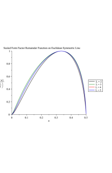
Figure 2: The $L$-loop form factor remainder function $R^{(L)}$ on the Euclidean line $(u,u,1-2u)$, normalized by its value at $u=1/3$. The four-loop curve is hidden under the five-loop one.

We can also study the behavior of the remainder function in scattering regions, where it becomes complex. To move from region I to region IIa, we let $\ln w\to\ln|w|-i\pi$ in the vicinity of the line $w=0$. We then use the coproduct formalism to integrate up from that line on the IIa branch. Similarly, to move from region I to region IIIa, we let $\ln u\to\ln|u|-i\pi$ and $\ln v\to\ln|v|-i\pi$ near the point $u=v=0$, and then integrate up from that point.

In Fig. 3(a), we plot the real part of the remainder function on the extension of the line $(u,u,1-2u)$ into the space-like scattering region IIa, for $u>1/2$, divided by its value at $u=1$. We see that the proportionality of the four- and five-loop results extends a bit into region IIa, but does not hold so strongly at larger values of $u$. In Fig. 3(b), we plot the imaginary part of the remainder function on the same IIa line, also normalized by the value of its real part at $u=1$.

$\frac{\text{Re }R^{(L)}(u,u,1-2u)}{\text{Re }R^{(L)}(1,1,-1)}$

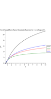
(a) .

$\frac{\text{Im }R^{(L)}(u,u,1-2u)}{\text{Re }R^{(L)}(1,1,-1)}$

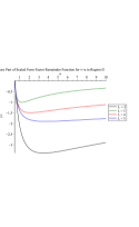
(b) .

Figure 3: Real (a) and imaginary (b) part of the $L$-loop form factor remainder function $R^{(L)}$ on the line $(u,u,1-2u)$ in scattering region IIa, $u>1/2$, normalized by the value of its real part at $u=1$.

The analogous plots for the extension of the line $(u,u,1-2u)$ into the time-like scattering region IIIa, with $u<0$, are given in Fig. 4(a) and Fig. 4(b). In this case, we normalize by the value of the real part at $u=-1$. In this region, the proportionality of the four- and five-loop remainder function holds to much larger values of $|u|$ than in region II.

$\frac{\text{Re }R^{(L)}(-u,-u,1+2u)}{\text{Re }R^{(L)}(-1,-1,3)}$

(a) .

$\frac{\text{Im }R^{(L)}(-u,-u,1+2u)}{\text{Re }R^{(L)}(-1,-1,3)}$

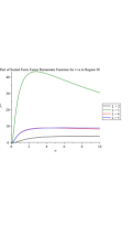
(b) .

Figure 4: Real (a) and imaginary (b) part of the $L$-loop form factor remainder function $R^{(L)}$ on the line $(u,u,1-2u)$ in scattering region IIIa, $u<0$, normalized by the value of its real part at $u=-1$.

Finally, we plot the remainder function in scattering region IIa again, but now on the line $u=1$, in Fig. 5(a) and Fig. 5(b). In this case the value at $v=\infty$ is real, and we normalize by that value.

$\frac{\text{Re }R^{(L)}(1,v,-v)}{R^{(L)}(1,\infty,-\infty)}$

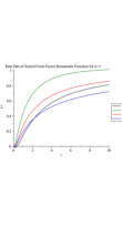
(a) .

$\frac{\text{Im }R^{(L)}(1,v,-v)}{R^{(L)}(1,\infty,-\infty)}$

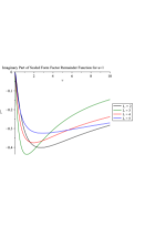
(b) .

Figure 5: Real (a) and imaginary (b) part of the $L$-loop form factor remainder function $R^{(L)}$ on the line $u=1$ in scattering region IIa, $v>0$, normalized by its (real) value at $v=\infty$.

5.2 Values at particular points

There are some distinguished points in the $(u,v)$ plane where the form factor remainder function takes on interesting analytic values. Of course, $R$ vanishes on the entire boundary of the Euclidean triangle, which includes the points $(u,v,w)=(1,0,0)$, $(0,1,0)$ and $(0,0,1)$. For the function space $\mathcal{M}$ as a whole, we expect only MZVs and logarithms of the two small variables at these points.

The point $(u,v,w)=(1,1,-1)$ lies at the intersection of the $u=1$ line and the $u=v$ line plotted earlier. From the representation of $\mathcal{M}$ on the $u=1$ line as HPLs of argument $v$ with weight vector elements $\{0,1,-1\}$, we know that the real and imaginary parts of $R$ at the point $(1,1,-1)$ must belong to the space of alternating sums. For example, the values at two and three loops are

$$R^{(2)}(1,1,-1) = 8\,{\rm Li}_{4}(1/2)+\frac{1}{3}\,\ln^{4}2+4\,\zeta_{2}\,\ln^{2}2-\frac{29}{4}\,\zeta_{4}$$ (74)

$$\hskip 0.0pt\hbox{}+i\pi\biggl{[}\frac{4}{3}\ln^{3}2+2\,\zeta_{2}\,\ln 2-2\,\zeta_{3}\biggr{]}\,,$$

$$R^{(3)}(1,1,-1) = -96\,{\rm Li}_{6}(1/2)+8\,\zeta_{2}\,{\rm Li}_{4}(1/2)-\frac{2}{15}\,\ln^{6}2-\frac{23}{3}\,\zeta_{2}\,\ln^{4}2-104\,\zeta_{4}\,\ln^{2}2$$ (75)

$$\hskip 0.0pt\hbox{}+24\,\zeta_{2}\,\zeta_{3}\,\ln 2+\frac{76}{3}\,\zeta_{6}+8\,(\zeta_{3})^{2}$$

$$\hskip 0.0pt\hbox{}+i\,\pi\,\biggl{[}32\,{\rm Li}_{5}(1/2)-\frac{2}{5}\,\ln^{5}2-\frac{4}{3}\,\zeta_{2}\,\ln^{3}2-4\,\zeta_{3}\,\ln^{2}2$$

$$\hskip 19.91684pt\hbox{}+\Bigl{(}16\,{\rm Li}_{4}(1/2)-19\,\zeta_{4}\Bigr{)}\,\ln 2+\frac{1}{4}\,\zeta_{5}+2\,\zeta_{2}\,\zeta_{3}\biggr{]}\,.$$

The values at four and five loops can be written in terms of an alternating-sum $f$-basis using HyperlogProcedures HyperlogProcedures , but the results are fairly lengthy. In Table 7 we present the numerical values of $R^{(L)}$ and of the ratio of successive loop orders $R^{(L)}/R^{(L-1)}$ at this point.

$L$	$R^{(L)}(1,1,-1)$	$R^{(L)}(1,1,-1)/R^{(L-1)}(1,1,-1)$
2	$-$0.4688118 + 1.0061952 $i$	–
3	$-$28.364132 + 27.844487 $i$	$+$33.528634 + 12.567654 $i$
4	546.09247 $-$ 697.38435 $i$	$-$22.095756 + 2.8958875 $i$
5	$-$8052.1673 + 11322.282 $i$	$-$15.668885 + 0.7234070 $i$

Table 7: The value of the remainder function at $(u,v,w)=(1,1,-1)$ at loop order $L$, as well as the ratio to the previous loop order. The five loop to four loop ratio is already not far from the asymptotic ratio of $-16$ for the cusp anomalous dimension.

When we take the limit $v\to\infty$ on the $u=1$ line, the remainder function becomes real, and the values belong to the space of MZVs:

$$R^{(2)}(1,\infty,-\infty) = -3\zeta_{4}\,,$$ (76)

$$R^{(3)}(1,\infty,-\infty) = -\frac{931}{12}\,\zeta_{6}+10\,(\zeta_{3})^{2}\,,$$ (77)

$$R^{(4)}(1,\infty,-\infty) = \frac{22193}{9}\,\zeta_{8}-352\,\zeta_{3}\,\zeta_{5}-20\,\zeta_{5,3}\,,$$ (78)

$$R^{(5)}(1,\infty,-\infty) = -\frac{941509787}{16800}\,\zeta_{10}-493\,\zeta_{4}\,(\zeta_{3})^{2}+920\,\zeta_{2}\,\zeta_{3}\,\zeta_{5}+\frac{29049}{7}\,(\zeta_{5})^{2}$$ (79)

$$\hskip 0.0pt\hbox{}+\frac{14843}{2}\,\zeta_{3}\,\zeta_{7}+\frac{124}{5}\,\zeta_{2}\,\zeta_{5,3}+\frac{1416}{7}\,\zeta_{7,3}\,.$$

We provide the numerical values, and the successive loop order ratios, in Table 8. The approach to the asymptotic cusp ratio of $-16$ is slower out at infinity than it is closer to the origin, which is similar to what is observed for six-point amplitudes Caron-Huot:2019vjl .

$L$	$R^{(L)}(1,\infty,-\infty)$	$R^{(L)}(1,\infty,-\infty)/R^{(L-1)}(1,\infty,-\infty)$
2	$-$3.2469697	–
3	$-$64.479458	$+$19.858349
4	2036.439992	$-$31.582771
5	$-$41521.8935	$-$20.389451

Table 8: The value of the remainder function at $(u,v,w)=(1,\infty,-\infty)$, i.e. the $v\to+\infty$ limit of the $u=1$ line, at loop order $L$, as well as the ratio to the previous loop order. The five-loop to four-loop ratio is not quite as close to the cusp asymptotic value of $-16$ as was the case at $(u,v,w)=(1,1,-1)$.

A second limit in which the remainder function becomes real and evaluates to MZVs is the limit where $u\to\pm\infty$ on the line $(u,u,1-2u)$. The value is independent of the sign of $u$; that is, it is the same whether we approach this point from within region IIa or region IIIa. Through five loops, the limit is

$$R^{(2)}(u,u,1-2u)\Big{|}_{u\to\infty} = -10\,\zeta_{4}\,,$$ (80)

$$R^{(3)}(u,u,1-2u)\Big{|}_{u\to\infty} = -\frac{371}{3}\,\zeta_{6}+8\,(\zeta_{3})^{2}\,,$$ (81)

$$R^{(4)}(u,u,1-2u)\Big{|}_{u\to\infty} = 5212\,\zeta_{8}+64\,\zeta_{2}\,(\zeta_{3})^{2}-160\,\zeta_{3}\,\zeta_{5}-24\,\zeta_{5,3}\,,$$ (82)

$$R^{(5)}(u,u,1-2u)\Big{|}_{u\to\infty} = -\frac{600943}{5}\,\zeta_{10}-672\,\zeta_{4}\,(\zeta_{3})^{2}-1280\,\zeta_{2}\,\zeta_{3}\,\zeta_{5}+708\,(\zeta_{5})^{2}$$ (83)

$$\hskip 0.0pt\hbox{}+1680\,\zeta_{3}\,\zeta_{7}+240\,\zeta_{2}\,\zeta_{5,3}+192\,\zeta_{7,3}\,.$$

The numerical values and the ratios to the previous loop order are shown in Table 9. The approach to the asymptotic cusp ratio is even slower here.

$L$	$R^{(L)}(u,u,1-2u)\Big{|}_{u\to\infty}$	$R^{(L)}(u,u,1-2u)/R^{(L-1)}(u,u,1-2u)\Big{|}_{u\to\infty}$
2	$-$10.823232	–
3	$-$114.25190	$+$10.556172
4	5185.0320798	$-$45.382458
5	$-$121169.4098	$-$23.369076

Table 9: The value of the $L$-loop remainder function at $(u,v,w)=(u,u,1-2u)$ with $u\to\infty$, as well as the ratio to the previous loop order.

The general conclusion of our numerical investigation is a rough consistency with the expected large-order asymptotics. The two-loop remainder function is a bit smaller, and has the opposite sign, than one might have expected from the higher-loop results, and the more strictly sign-alternating behavior of six-and seven-point amplitude remainder functions Dixon:2013eka ; Dixon:2014voa ; Caron-Huot:2019vjl ; Dixon:2020cnr . Also, the form factor remainder function tends to a constant at infinity, which has interesting consequences for the high-energy or Regge limit, as we will mention in section 7.

6 Multi-Loop One-Mass Four-Point Integrals

As mentioned in section 2.2, the ES-like adjacency restriction (30), which is critical to defining the function space $\mathcal{M}$, was first motivated by its appearance in the form factor (as opposed to the remainder function) computed in ref. Brandhuber:2012vm . We have also inspected several other three-point form factors, or amplitudes involving a Higgs boson and three gluons, that are available in the literature Gehrmann:2011aa ; Brandhuber:2012vm ; Brandhuber:2014ica ; Brandhuber:2017bkg . All obey the same ES-like restriction. The constraint (30) has no effect until weight three, because $1-u$ cannot appear until the second entry, but it can be seen in the weight-three and -four functions in these references.

All of the quantities in question are linear combinations of a class of two-loop master integrals associated with four-point processes with one massive and three massless external legs, and all massless internal lines, for both planar and non-planar topologies. The master integrals for these topologies were first computed through weight four in refs. Gehrmann:2000zt ; Gehrmann:2001ck . More recently they have been expanded further in the dimensional regularization parameter $\epsilon$, through weights five Duhr:2014nda and six Mistlbergerprivate . Examining these two-loop master integrals through weight six Mistlbergerprivate , we find that they all lie within $\mathcal{M}$. There are 89 different master integrals. At weight four, 69 symbols and 79 functions of the 89 are linearly independent, while there are $3^{4}=81$ symbols and (from Table 4) 94 functions in $\mathcal{M}_{4}$. Thus only 12 of the weight-four symbols in $\mathcal{M}$ are not captured by the two-loop master integrals. At weight five, there are 72 and 86 independent symbols and functions, respectively. (These numbers depend a bit on how the integrals are normalized; shifting them all by factors like $(u_{i})^{\epsilon}$ can change the number of independent higher-weight functions.) We expect much more of the space $\mathcal{M}$ at weights five and six to be filled out by three-loop integrals.

Based on the fact that all the two-loop master integrals are in $\mathcal{M}$, as well as the planar ${\cal N}=4$ sYM form factors through five loops, we expect that this space contains all master integrals for the same topologies, one massive and three massless external legs, and all massless external lines, planar and non-planar, to higher loop orders. However, for reasons discussed in the “note added”, we don’t expect this statement to be true to arbitrary loop order. If our expectation is true, then any four-point amplitude with these kinematics, for example subleading-in-$N$ corrections in ${\cal N}=4$ sYM, as well as QCD corrections to amplitudes for $gg\to Hg$ (in the heavy-top limit), $qg\to Zq$, and $e^{+}e^{-}\to q\bar{q}g$, can be expressed to three loops, possibly further, in terms of the transcendental functions in $\mathcal{M}$. All different weights up to $2L$ can be expected to appear at $L$ loops in QCD, and the rational-function prefactors in front of these functions, especially the lower-weight ones, can be expected to become rather intricate. Nevertheless, this would be a remarkable property for a large class of high-order amplitudes in massless theories to exhibit.

7 Conclusions and outlook

In this paper, we have bootstrapped the three-point form factor of the chiral part of the stress-tensor supermultiplet in planar $\mathcal{N}=4$ sYM theory through five loops, extending the state of the art by three loop orders. To carry out this bootstrap, we have utilized new boundary data coming from the OPE in the near-collinear limit of these form factors Sever:2020jjx ; Toappear1 ; Toappear2 . The OPE also provides important cross-checks on our results. On the other hand, the information about subleading logarithms in $T$ at order $T^{2}$ coming from our results also assisted the determination of the higher-order behavior of the form factor transition. The integrability-based bootstrap and the perturbative form factor bootstrap thus complement each other quite nicely.

These new form factor results provide a novel glimpse into the mathematical structure of gauge theory at high loop orders, complementing our rapidly-developing understanding of the mathematical structure of multi-loop amplitudes. In particular, we have observed novel extended-Steinmann-like constraints (30) that are obeyed by the finite part of the form factor $\mathcal{E}^{(L)}$. Similar to the extended Steinmann relations for amplitudes Caron-Huot:2019bsq , we do not have a full proof of these relations based on physical principles. It would thus be interesting to elucidate the origin of these restrictions, perhaps using the types of methods employed in refs. Abreu:2014cla ; Bloch:2015efx ; Abreu:2017ptx ; Bourjaily:2019exo ; Bourjaily:2020wvq ; Benincasa:2020aoj .

We have also observed that the functions $\mathcal{E}^{(L)}$ satisfy multiple-final-entry conditions. Namely, the double coproduct entries of $\mathcal{E}^{(L)}$ satisfy relation (64), and its dihedral images, through at least five loops. It would be interesting to see if these relations could be derived using the $\bar{Q}$ equation CaronHuot:2011ky ; CaronHuot:2011kk . Similarly, the triple coproduct entries of $\mathcal{E}^{(L)}$ satisfy relations (66)–(70), and their dihedral images, through the same loop order. It is worth noting that the six-point amplitude also satisfies next-to-final-entry conditions Dixon:2015iva ; however, when the extended Steinmann relations are used to build up the space of hexagon functions, these conditions are automatically satisfied Caron-Huot:2019vjl . As seen in Table 3 and Table 5, the multiple-final-entry constraints that we observe are not redundant with the other general assumptions we currently build into our ansatz.

In addition to exhibiting interesting mathematical structure, these form factors should be closely related to quantities of phenomenological interest. In particular, we expect the remainder function $R^{(L)}$ to match the maximally transcendental parts of the $gg\to Hg$ and $H\to ggg$ amplitude remainder functions in the heavy-top limit of QCD. Additionally, for the reasons described in section 6, we believe that the lower-transcendentality functions appearing in these QCD amplitudes at three loops will be contained in the form factor space $\mathcal{M}$, although they will have more complicated rational prefactors. These form factors, and the function space $\mathcal{M}$, are thus important for future studies of the Higgs boson, among other LHC processes.

An interesting avenue for future work is to study the high-energy or Regge behavior of four-point scattering involving a colorless operator. In the case of four-gluon scattering, where the remainder function vanishes, the BDS formula Bern:2005iz is consistent with Regge behavior being controlled by the cusp and collinear anomalous dimensions Drummond:2007aua ; Naculich:2007ub . In the present case, the remainder function does not vanish in the scattering region II (space-like operator), but as we saw in section 5.2, it goes to a real constant as $v\to\infty$ for $u=1$, or for $u=v$. This constancy follows from the final-entry condition, $R^{u_{i}}+R^{1-u_{i}}=0$. For $u\ll v$, this region is the high-energy limit $s_{23}\gg s_{12},q^{2}$. The logarithmic growth with energy again is captured by the infrared-divergent terms, as well as $E^{(1)}$, which have been removed from the remainder function. However, there will also be an impact factor, which does not depend on $s_{23}$, but does depend on the dimensionless ratio $u=s_{12}/q^{2}$. It can be extracted from the remainder function to high loop orders. Similar remarks apply to scattering region III (the time-like operator).

We have defined the form factor function space $\mathcal{M}$ to have the analytic properties expected of a generic Feynman integral that draws from the $\mathcal{S}_{3}$ symbol alphabet, and to obey the extended-Steinmann-like relations (30). In order to carry out our bootstrap, we have iteratively constructed $\mathcal{M}$ through weight eight. While the space $\mathcal{M}$ involve fewer symbol letters than the hexagon function space $\mathcal{H}$, we find that its dimension grows faster with the transcendental weight $w$, namely as $3^{w}$ — compared to $\sim 1.8^{w}$ in the hexagon case. However, the clean growth of the function space with the weight and the simpler letters make $\mathcal{M}$ an ideal testing ground for constructing the function space in a closed form.

In fact, we have found that the function $\mathcal{E}$ is contained in the smaller subspace $\mathcal{C}\subset\mathcal{M}$. We expect this space to be crucial for going beyond five-loop order in-progress , but we do not yet have a bottom-up, or first-principles, construction of $\mathcal{C}$.

It would also be interesting to bootstrap form factors with a larger number of points $n$. In particular, a non-trivial NMHV form factor is first encountered at $n=4$. Higher-point form factors for $\operatorname{tr}(F_{SD}^{2})$ factorize onto $n$ gluon scattering amplitudes for $n\geq 4$. Since these amplitudes do not obey a maximal-transcendentality principle, we also do not expect such a principle to hold between ${\cal N}=4$ sYM form factors and QCD Higgs amplitudes, beyond $n=3$.

Finally, it would be interesting to bootstrap form factors of different operators. Possible operators include those studied in refs. Bork:2010wf ; Engelund:2012re ; Brandhuber:2014ica ; Wilhelm:2014qua ; Nandan:2014oga ; Loebbert:2015ova ; Brandhuber:2016fni ; Loebbert:2016xkw ; Caron-Huot:2016cwu ; Ahmed:2016vgl ; Banerjee:2016kri ; Huber:2019fea ; Lin:2020dyj . In particular, in the case of the two-loop three-point form factor for $\operatorname{tr}(F^{3})$ it has been shown that the next-to-leading order contribution to the Higgs amplitude remainder in the heavy-top limit of QCD shares its maximally transcendental part with its counterpart in $\mathcal{N}=4$ sYM theory Brandhuber:2017bkg ; Brandhuber:2018xzk ; Brandhuber:2018kqb ; Jin:2018fak . These form factors are liable to have just as interesting a structure at higher loops as the form factor we have studied in this work.

Note Added: The initial version of this paper included the conjecture that the transcendental functions appearing in four-point one-mass amplitudes would be contained in the $\mathcal{M}$ space to all loop orders. After it appeared, we were reminded by Erik Panzer that non-polylogarithmic periods are known to appear in massless $\phi^{4}$ theory by eight loops Brown:2010bw ; Brown:2013wn ; Panzer:2016snt . Because these period integrals can be converted to propagator integrals by injecting external momentum, and since propagator integrals are contained within four-point one-mass integrals, the polylogarithmic conjecture we originally put forward must fail at higher loop orders (in generic massless quantum field theories).

Appendix A Pentaladder integrals

The pentaladder integrals, or pentabox ladder integrals, belong to both the form factor space $\mathcal{M}$ and the heptagon function space. As such, they provide a way of understanding the ES-like adjacency restrictions for some of the functions in $\mathcal{M}$, in terms of adjacency restrictions which follow from extended Steinmann relations for heptagon functions, as we will discuss in this appendix.

The class of pentaladder integrals depicted in Fig. 6 was first considered in ref. Drummond:2010cz . With the inclusion of a numerator associated with the pentagon loop (which is depicted graphically by a dashed line), they are rendered infrared finite and dual conformally invariant (DCI). Starting from the one-loop pentagon integral,

$${\cal I}_{pl}^{(1)}(x_{1},x_{2},x_{3},x_{4},x_{6})=\frac{x_{14}^{2}x_{26}^{2}x_{36}^{2}}{x_{6a}^{2}}\int\frac{d^{4}x_{r}}{i\pi^{2}}\frac{x_{ar}^{2}}{x_{1r}^{2}x_{2r}^{2}x_{3r}^{2}x_{4r}^{2}x_{6r}^{2}}\,,$$ (84)

where $x_{a}$ is the dual point that satisfies the null-separation conditions $x_{a1}^{2}=x_{a2}^{2}=x_{a3}^{2}=x_{a4}^{2}=0$, the $L$-loop pentaladder integral can be constructed iteratively by including $L{-}1$ further integrations of the form

$${\cal I}_{pl}^{(L)}(x_{1},x_{2},x_{3},x_{4},x_{6})=\frac{x_{14}^{2}x_{26}^{2}x_{36}^{2}}{x_{6a}^{2}}\int\frac{d^{4}x_{r}}{i\pi^{2}}\frac{x_{ar}^{2}}{x_{1r}^{2}x_{2r}^{2}x_{3r}^{2}x_{4r}^{2}x_{6r}^{2}}{\cal I}_{pl}^{(L-1)}(x_{1},x_{2},x_{3},x_{4},x_{r})\,.$$ (85)

These integrals depend on the pair of cross-ratios

$$U=\frac{x_{46}^{2}x_{13}^{2}}{x_{36}^{2}x_{14}^{2}}\,,\qquad V=\frac{x_{16}^{2}x_{24}^{2}}{x_{26}^{2}x_{14}^{2}}\,,$$ (86)

which describe a two-dimensional subspace of seven-particle kinematics.

(300,140) dot_size0.18mm (.115w,.5h)p1 (.255w,.86h)p2 (.41w,.68h)p3 (.54w,.68h)p4 (.67w,.68h)p5 (.8w,.68h)p7 (.8w,.32h)p9 (.67w,.32h)p11 (.54w,.32h)p12 (.41w,.32h)p13 (.255w,.14h)p14 (.575w,.5h)d1 (.605w,.5h)d2 (.635w,.5h)d3 (.04w,.5h)e1 (.23w,1.0h)e2 (0.9w,0.85h)e3 (0.93w,0.75h)e4 (0.93w,0.25h)e5 (0.9w,0.15h)e6 (.23w,0.0h)e7 (.12w,.84h)l1 (.59w,.85h)l2 (0.9w,.5h)l34 (.59w,.15h)l5 (.12w,.16h)l6 plain, width=.2mmp1,p2 plain, width=.2mmp2,p3 plain, width=.2mmp3,p4 plain, width=.2mmp4,p5 plain, width=.2mmp5,p7 plain, width=.2mmp7,p9 plain, width=.2mmp9,p11 plain, width=.2mmp11,p12 plain, width=.2mmp12,p13 plain, width=.2mmp13,p14 plain, width=.2mmp14,p1 dashes, width=.2mmp2,p14 plain, width=.2mmp3,p13 plain, width=.2mmp4,p12 plain, width=.2mmp5,p11 plain, width=.2mmp1,e1 plain, width=.2mmp2,e2 plain, width=.2mmp7,e3 plain, width=.2mmp7,e4 plain, width=.2mmp9,e5 plain, width=.2mmp9,e6 plain, width=.2mmp14,e7 d1 d2 d3 label=$x_{3}$, label.dist=.1cml1 label=$x_{4}$, label.dist=.1cml2 label=$x_{6}$, label.dist=.1cml34 label=$x_{1}$, label.dist=.1cml5 label=$x_{2}$, label.dist=.1cml6

Figure 6: The seven-point pentabox ladder integral, labeled by dual coordinates, in which the box ladder involves $L-1$ loops. The dashed line represents a numerator factor that renders the integral DCI and infrared finite. This class of integrals maps into the space of functions relevant for the three-point form factor in the limit $x_{6}\to\infty$.

An important aspect of this class of integrals is that adjacent loop orders are related to each other by a second-order differential equation Drummond:2010cz . Specifically, defining the function

$$\Psi^{(L)}(U,V)=(1-U-V)\,{\cal I}_{pl}^{(L)}(x_{1},x_{2},x_{3},x_{4},x_{6})\,,$$ (87)

we have that

$$UV(1-U-V)\partial_{V}\partial_{U}\Psi^{(L)}(U,V)=\Psi^{(L-1)}(U,V)\,.$$ (88)

Using this relation, these integrals have been computed to high loop order and resummed in the coupling Caron-Huot:2018dsv . As a result, explicit polylogarithmic expressions for these integrals are available through eight loops.

These integrals also turn out to be relevant to the space of functions entering the three-point form factors in this paper. To see how, consider the limit in which the dual point $x_{6}$ is sent to infinity. In this limit, the seven-point cross ratios (86) simplify to ratios that only depend on three external momenta:

$$U\xrightarrow[]{x_{6}\to\infty}\frac{x_{13}^{2}}{x_{14}^{2}}=\frac{s_{12}}{s_{123}}=u\,,\qquad V\xrightarrow[]{x_{6}\to\infty}\frac{x_{24}^{2}}{x_{14}^{2}}=\frac{s_{23}}{s_{123}}=v\,.$$ (89)

Thus, these variables map directly to the variables $u$ and $v$ defined in eq. (4), while all kinematic dependence on the box end of the ladders drops out.

Since the variables $U$ and $V$ each remain finite in the limit (89), the functional form of $\Psi^{(L)}$ does not change, and we can directly check whether they have the right properties to contribute to the form factor $\mathcal{F}_{3}^{\rm MHV}$. As it turns out, they only draw from the five-letter subset

$$\{u,\,v,\,1-u,\,1-v,\,1-u-v\}$$ (90)

of the six-letter symbol alphabet (21). Also, they obey the same extended Steinmann constraints as the form factor space $\mathcal{M}$, insofar as the two letters $1{-}u$ and $1{-}v$ never appear sequentially in their symbols. Since only the letters $u$ and $v$ can appear in the first entry in seven-particle kinematics, these functions also satisfy the first-entry condition relevant for form factors. Thus, we see that the functions $\Psi^{(L)}(u,v)$ have all of the right properties to appear in the space of functions $\mathcal{M}$ constructed in section 3.

The differential equation (88) implies the single coproduct relations,

$$\Psi^{w}=\Psi^{u}+\Psi^{1-u}=\Psi^{v}+\Psi^{1-v}=0,$$ (91)

and the additional double coproduct ones,

$$\Psi^{1-u,1-v} = \Psi^{1-v,1-u}=0,$$ (92)

$$\Psi^{u,v} = \Psi^{v,u}=-\Psi^{1-u-v,u}=-\Psi^{1-u-v,v}=\Psi^{(L-1)}\,,$$ (93)

where we have dropped the $(L)$ superscript on $\Psi^{(L)}$ for clarity. Using these relations, the flip symmetry $\Psi^{(L)}(u,v)=\Psi^{(L)}(v,u)$, and the vanishing of $\Psi$ in the collinear limit $w=1-u-v\to 0$, it is easy to locate the pentabox ladder integrals in $\mathcal{M}$; we have done so through five loops.

The extended-Steinmann-like constraints we have observed for the form factor space $\mathcal{M}$ do not seem to have a direct physical explanation, based on causality, within that space alone. On the other hand, when $\Psi^{(L)}\in\mathcal{M}$ is interpreted as a pentaladder integral in heptagon kinematics, the constraints follow from the extended Steinmann relations in planar $\mathcal{N}=4$ sYM theory Dixon:2016nkn ; Caron-Huot:2019bsq , which have a causal interpretation. This connection can be seen most easily by building the full space of polylogarithms with the alphabet (90)—interpreted as heptagon letters via the definitions (86)—that satisfy the first-entry and extended Steinmann conditions. This construction generates the $\mathcal{P}$ subspace of the form factor space $\mathcal{M}$, which has dimension

$$d_{\mathcal{P},\,\text{symb}}(t)\equiv\sum_{w=1}^{\infty}d_{\mathcal{P}}(w)t^{w}=\frac{1-t-2t^{2}+t^{3}}{(1-2t)(1-t-t^{2})}=1+2t+3t^{2}+6t^{3}+11t^{4}+\cdots\,$$ (94)

at symbol level. Notice that only two functions appear at weight one, consistent with the above comment that $1-u-v$ does not satisfy the first-entry condition in heptagon kinematics. Moreover, at weight two, only the functions

$$\textrm{Li}_{2}(1-1/u),\quad\textrm{Li}_{2}(1-1/v),\quad\ln^{2}(u/v),$$ (95)

survive after applying the heptagon Steinmann conditions. As has been previously observed in heptagon kinematics, imposing the extended Steinmann relations at each higher weight also implies cluster adjacency Drummond:2017ssj ; Drummond:2018dfd ; Golden:2019kks , even though the latter condition seems to imply more constraints.

In terms of the labelling of the heptagon cross ratios $u_{i}$, and the heptagon $g$ letters described in ref. Dixon:2020cnr , the five letters (90) become

$$u = u_{2}u_{6}=g_{1,2}\,g_{1,6}\,,\qquad v=u_{4}u_{7}=g_{1,4}\,g_{1,7}\,,$$

$$1-u = g_{3,4}\,,\qquad 1-v=g_{3,2}\,,\qquad 1-u-v=g_{4,3}\,.$$ (96)

To restate the previous connection in terms of these letters: the letters $g_{3,i}$ and $g_{3,i+2}$ are never found adjacent to each other in the extended Steinmann heptagon function space.

It would be very interesting to find a constructive description of the space $\mathcal{P}$, perhaps as a prelude to finding one for $\mathcal{M}$ or $\mathcal{C}$. We leave this to future work.

Appendix B Near-collinear limit at orders $T^{2}$ and $T^{4}$

In this appendix, we describe further the structure of the near-collinear expansion of the remainder function discussed in section 4.1, providing explicit results at two and three loops.

The near-collinear expansion of the three-point remainder function $R\equiv R_{3}$ in $T$ has the form,

$$R^{(L)}(T,S)=\sum_{j=1}^{\infty}\sum_{k=0}^{L-1}T^{2j}\,\ln^{k}T\,R_{j,k}^{(L)}(S)\,.$$ (97)

From the FFOPE side, the $T^{2}$ terms are completely determined, as are essentially all of the $T^{4}$ terms. As mentioned in section 4.1, the FFOPE results are generated as a high-order series expansion around $S=0$. One can construct an ansatz for the closed-form dependence on $S$ in terms of HPLs up to a certain weight with suitable rational-function prefactors. With enough terms in the series expansion, one can fix all of the coefficients in the ansatz.

Alternatively, it is straightforward to obtain the complete dependence on $S$ by using the coproduct representation to compute the $v$ (or $T$) derivative of each function in $\mathcal{M}$ in terms of lower-weight functions. The integration in $T$ is trivial to do, order-by-order in $T$, given the expansion (97). The HPLs are generated by the $T^{0}$ term in the expansion, where the derivative in $u$ has to be integrated up (at least for the terms with no $\ln T$), but this is also straightforward. After constructing the near-collinear limits of all the functions, the results for $E$ or ${\cal E}$, and then for $R$, can be obtained, in principle to any power of $T^{2}$.

Here we provide some terms at order $T^{2}$ and $T^{4}$. It is convenient to take the argument of the harmonic polylogarithms to be $x=-S^{2}$. At order $T^{2}$, we can separate out the rational prefactors by writing

$$R_{1,k}^{(L)}=\frac{(1-x)^{2}}{x}A^{(L)}_{k}+(1-x)B^{(L)}_{k}+C^{(L)}_{k}\,,$$ (98)

where $A^{(L)}_{k}$, $B^{(L)}_{k}$ and $C^{(L)}_{k}$ are pure functions, although not of uniform weight. This particular decomposition is useful because the maximum weight of $A^{(L)}_{k}$ is $2L-k-1$, whereas $B^{(L)}_{k}$ and $C^{(L)}_{k}$ turn out to have a maximal weight of $2L-k-2$.

At two loops, these functions are given by

$$A^{(2)}_{1} = -8\,H_{1}(x)\,\ln(-x)-16\,H_{1,1}(x)-8\,H_{1}(x)\,,$$ (99)

$$B^{(2)}_{1} = 8\,\ln(-x)\,,$$ (100)

$$C^{(2)}_{1} = 8\,,$$ (101)

$$A^{(2)}_{0} = 4\,\bigl{[}2\,H_{1,1}(x)+H_{1}(x)\bigr{]}\,\ln(-x)+8\,H_{0,0,1}(x)+16\,H_{1,1,1}(x)-8\,\zeta_{2}\,H_{1}(x)$$ (102)

$$\hskip 0.0pt\hbox{}+8\,H_{1,1}(x)+4\,H_{1}(x)\,,$$

$$B^{(2)}_{0} = -4\,\ln(-x)\,,$$ (103)

$$C^{(2)}_{0} = 8\,\zeta_{2}-12\,.$$ (104)

At three loops, suppressing now the argument $x$ of the HPLs, we have

$$A^{(3)}_{2} = -12\,H_{1}\,\ln^{2}(-x)-32\,\bigl{[}2\,H_{1,1}+H_{1}\bigr{]}\,\ln(-x)+8\,H_{0,0,1}-128\,H_{1,1,1}-8\,\zeta_{2}\,H_{1}$$ (105)

$$\hskip 0.0pt\hbox{}-64\,H_{1,1}-32\,H_{1}\,,$$

$$B^{(3)}_{2} = 32\,\ln(-x)\,,$$ (106)

$$C^{(3)}_{2} = 12\,\ln^{2}(-x)+8\,\zeta_{2}+24\,,$$ (107)

$$A^{(3)}_{1} = 12\,\bigl{[}2\,H_{1,1}+H_{1}\bigr{]}\,\ln^{2}(-x)+4\,\bigl{[}2\,H_{1,0,1}+4\,H_{0,0,1}+2\,H_{0,1,1}+48\,H_{1,1,1}$$ (108)

$$\hskip 14.22636pt\hbox{}+6\,\zeta_{2}\,H_{1}+24\,H_{1,1}+11\,H_{1}\bigr{]}\,\ln(-x)$$

$$\hskip 0.0pt\hbox{}+24\,H_{1,0,0,1}+24\,H_{0,1,0,1}+48\,H_{0,0,1,1}+384\,H_{1,1,1,1}$$

$$\hskip 0.0pt\hbox{}+8\,\zeta_{2}\,\bigl{[}2\,H_{1,1}+H_{1}\bigr{]}-8\,\zeta_{3}\,H_{1}+24\,H_{0,0,1}+192\,H_{1,1,1}$$

$$\hskip 0.0pt\hbox{}+12\,H_{0,1}+96\,H_{1,1}+60\,H_{1}\,,$$

$$B^{(3)}_{1} = 2\,\ln^{2}(-x)+\bigl{[}-32\,\zeta_{2}-8\,H_{1}-60\bigr{]}\,\ln(-x)+24\,H_{0,1}+12\,\zeta_{2}\,,$$ (109)

$$C^{(3)}_{1} = -14\,\ln^{2}(-x)+\bigl{[}-8\,H_{0,1}+8\,\zeta_{2}\bigr{]}\,\ln(-x)+24\,H_{0,0,1}+8\,\zeta_{3}-20\,\zeta_{2}-96\,,$$ (110)

$$A^{(3)}_{0} = \bigl{[}-24\,H_{1,1,1}-2\,H_{1,0,1}+2\,H_{0,0,1}-2\,H_{0,1,1}-2\,\zeta_{2}\,H_{1}-12\,H_{1,1}-5\,H_{1}\bigr{]}\,\ln^{2}(-x)$$ (111)

$$\hskip 0.0pt\hbox{}+\bigl{[}-12\,H_{0,1,1,1}-8\,H_{1,0,0,1}-8\,H_{0,1,0,1}-16\,H_{0,0,1,1}-8\,H_{1,1,0,1}-12\,H_{1,0,1,1}$$

$$\hskip 14.22636pt\hbox{}-192\,H_{1,1,1,1}-12\,\zeta_{2}\,(2\,H_{1,1}+H_{1})-4\,\zeta_{3}\,H_{1}-4\,H_{1,0,1}-4\,H_{0,1,1}-8\,H_{0,0,1}$$

$$\hskip 14.22636pt\hbox{}-96\,H_{1,1,1}-4\,H_{0,1}-46\,H_{1,1}-24\,H_{1}\bigr{]}\,\ln(-x)$$

$$\hskip 0.0pt\hbox{}-48\,H_{0,0,1,1,1}-72\,H_{0,0,0,0,1}-12\,H_{0,0,0,1,1}-24\,H_{1,1,0,0,1}-24\,H_{1,0,1,0,1}$$

$$\hskip 0.0pt\hbox{}-36\,H_{1,0,0,1,1}-24\,H_{0,1,1,0,1}-12\,H_{1,0,0,0,1}-12\,H_{0,1,0,0,1}-12\,H_{0,0,1,0,1}$$

$$\hskip 0.0pt\hbox{}-36\,H_{0,1,0,1,1}-384\,H_{1,1,1,1,1}+16\,\zeta_{2}\,\bigl{[}H_{0,0,1}-H_{1,1,1}\bigr{]}+4\,\zeta_{3}\,\bigl{[}2\,H_{1,1}+H_{1}\bigr{]}$$

$$\hskip 0.0pt\hbox{}+77\,\zeta_{4}\,H_{1}-12\,H_{1,0,0,1}-12\,H_{0,1,0,1}-24\,H_{0,0,1,1}-192\,H_{1,1,1,1}-8\,\zeta_{2}\,H_{1,1}$$

$$\hskip 0.0pt\hbox{}-6\,H_{0,0,1}-6\,H_{0,1}-6\,H_{0,1,1}-96\,H_{1,1,1}-54\,H_{1,1}-4\,\zeta_{2}\,H_{1}-36\,H_{1}\,,$$

$$B^{(3)}_{0} = 2\,\ln^{2}(-x)\,H_{1}+\bigl{[}-6\,H_{0,1}+4\,H_{1,1}+6\,H_{1}+14\,\zeta_{2}+36\bigr{]}\,\ln(-x)$$ (112)

$$\hskip 0.0pt\hbox{}+6\,H_{0,0,1}-12\,H_{0,1}-12\,H_{0,1,1}+6\,\zeta_{3}-6\,\zeta_{2}\,,$$

$$C^{(3)}_{0} = \bigl{[}2\,H_{0,1}+2\,\zeta_{2}+3\bigr{]}\,\ln^{2}(-x)+\bigl{[}-8\,H_{0,0,1}+4\,H_{0,1,1}+2\,H_{0,1}+4\,\zeta_{3}-2\,\zeta_{2}\bigr{]}\,\ln(-x)$$ (113)

$$\hskip 0.0pt\hbox{}-12\,H_{0,0,1,1}+12\,H_{0,0,0,1}-6\,H_{0,0,1}-77\,\zeta_{4}-10\,\zeta_{3}-6\,\zeta_{2}+120\,.$$

The expressions at four and five loops may be found in the ancillary file T2terms.txt.

Similarly, at order $T^{4}$, the rational prefactors can be separated out by letting

$$R_{2,k}^{(L)} = \frac{(1-x)(1+x+3x^{2}-x^{3})}{x^{2}}D^{(L)}_{k}+\frac{(1-x)^{2}(1+2x-x^{2})}{x^{2}}E^{(L)}_{k}+\frac{(1-x)^{4}}{x^{2}}F^{(L)}_{k}$$ (114)

$$\hskip 0.0pt\hbox{}+(1-x)G^{(L)}_{k}+K^{(L)}_{k}\,,$$

where $D^{(L)}_{k}$, $\ldots$, $K^{(L)}_{k}$ are pure functions, although again not of uniform weight. The maximum weight of $D^{(L)}_{k}$ is $2L-k-1$, while the other coefficients have at most one weight lower.

At two loops, these functions are given by

$$D^{(2)}_{1} = -4\,H_{1}\,\ln(-x)-8\,H_{1,1}+\frac{1}{2}\,,$$ (115)

$$E^{(2)}_{1} = \ln(-x)\,,$$ (116)

$$F^{(2)}_{1} = -\ln(-x)-2\,H_{1}-\frac{1}{2}\,,$$ (117)

$$G^{(2)}_{1} = 4\,\ln(-x)-2\,,$$ (118)

$$K^{(2)}_{1} = 8\,\ln(-x)+1\,,$$ (119)

$$D^{(2)}_{0} = 4\,H_{1,1}\,\ln(-x)+8\,H_{1,1,1}+4\,H_{0,0,1}-\zeta_{2}\,\bigl{[}4\,H_{1}-3\bigr{]}+H_{1}-\frac{1}{8}\,,$$ (120)

$$E^{(2)}_{0} = \biggl{[}2\,H_{1}-\frac{1}{4}\biggr{]}\,\ln(-x)-4\,H_{0,1}-2\,\zeta_{2}\,,$$ (121)

$$F^{(2)}_{0} = -\biggl{[}H_{1}-\frac{1}{4}\biggr{]}\,\ln(-x)-2\,H_{1,1}-\zeta_{2}-\frac{1}{2}\,H_{1}+\frac{1}{8}\,,$$ (122)

$$G^{(2)}_{0} = -5\,\ln(-x)-4\,\zeta_{2}-4\,H_{1}+\frac{1}{2}\,,$$ (123)

$$K^{(2)}_{0} = -4\,\ln(-x)-2\,\zeta_{2}-\frac{7}{4}\,.$$ (124)

At three loops, the $\ln^{2}T$ coefficients are

$$D^{(3)}_{2} = -\biggl{[}6\,H_{1}-\frac{9}{2}\biggr{]}\,\ln^{2}(-x)-32\,H_{1,1}\,\ln(-x)-64\,H_{1,1,1}+4\,H_{0,0,1}$$ (125)

$$\hskip 0.0pt\hbox{}-\zeta_{2}\,(4\,H_{1}-3)+\frac{3}{2}\,,$$

$$E^{(3)}_{2} = -3\,\ln^{2}(-x)-(4\,H_{1}-3)\,\ln(-x)-4\,H_{0,1}-2\,\zeta_{2}\,,$$ (126)

$$F^{(3)}_{2} = -\frac{3}{2}\,\ln^{2}(-x)-(8\,H_{1}+3)\,\ln(-x)-16\,H_{1,1}-6\,H_{1}-\zeta_{2}-\frac{3}{2}\,,$$ (127)

$$G^{(3)}_{2} = -6\,\ln^{2}(-x)+12\,\ln(-x)-4\,\zeta_{2}-6\,,$$ (128)

$$K^{(3)}_{2} = -3\,\ln^{2}(-x)+8\,\ln(-x)-2\,\zeta_{2}-\frac{1}{2}\,.$$ (129)

The remaining three-loop $T^{4}$ coefficients, and the four- and five-loop ones, can be found in the ancillary file T4terms.txt.

References

- (1) C. Anastasiou, C. Duhr, F. Dulat, F. Herzog and B. Mistlberger, Higgs Boson Gluon-Fusion Production in QCD at Three Loops, Phys. Rev. Lett. 114 (2015) 212001 [1503.06056].
- (2) B. Mistlberger, Higgs boson production at hadron colliders at N3LO in QCD, JHEP 05 (2018) 028 [1802.00833].
- (3) F. Wilczek, Decays of Heavy Vector Mesons Into Higgs Particles, Phys. Rev. Lett. 39 (1977) 1304.
- (4) M. A. Shifman, A. Vainshtein and V. I. Zakharov, Remarks on Higgs Boson Interactions with Nucleons, Phys. Lett. B 78 (1978) 443.
- (5) L. J. Dixon, E. Glover and V. V. Khoze, MHV rules for Higgs plus multi-gluon amplitudes, JHEP 12 (2004) 015 [hep-th/0411092].
- (6) T. Gehrmann, M. Jaquier, E. Glover and A. Koukoutsakis, Two-Loop QCD Corrections to the Helicity Amplitudes for 3 partons, JHEP 02 (2012) 056 [1112.3554].
- (7) Z. Bern, L. J. Dixon, D. A. Kosower, R. Roiban, M. Spradlin, C. Vergu et al., The Two-Loop Six-Gluon MHV Amplitude in Maximally Supersymmetric Yang-Mills Theory, Phys. Rev. D78 (2008) 045007 [0803.1465].
- (8) J. Drummond, J. Henn, G. Korchemsky and E. Sokatchev, Hexagon Wilson loop = six-gluon MHV amplitude, Nucl.Phys. B815 (2009) 142 [0803.1466].
- (9) A. Brandhuber, G. Travaglini and G. Yang, Analytic two-loop form factors in SYM, JHEP 05 (2012) 082 [1201.4170].
- (10) A. Kotikov and L. Lipatov, DGLAP and BFKL evolution equations in the supersymmetric gauge theory, in 35th Annual Winter School on Nuclear and Particle Physics, 12, 2001, hep-ph/0112346.
- (11) A. Kotikov and L. Lipatov, DGLAP and BFKL equations in the supersymmetric gauge theory, Nucl. Phys. B 661 (2003) 19 [hep-ph/0208220].
- (12) A. Kotikov, L. Lipatov, A. Onishchenko and V. Velizhanin, Three loop universal anomalous dimension of the Wilson operators in SUSY Yang-Mills model, Phys. Lett. B 595 (2004) 521 [hep-th/0404092].
- (13) A. Kotikov, L. Lipatov, A. Rej, M. Staudacher and V. Velizhanin, Dressing and wrapping, J. Stat. Mech. 0710 (2007) P10003 [0704.3586].
- (14) A. Brandhuber, B. Spence, G. Travaglini and G. Yang, Form Factors in Super Yang-Mills and Periodic Wilson Loops, JHEP 01 (2011) 134 [1011.1899].
- (15) A. Brandhuber, Ö. Gürdoğan, R. Mooney, G. Travaglini and G. Yang, Harmony of Super Form Factors, JHEP 10 (2011) 046 [1107.5067].
- (16) A. Bolshov, L. Bork and A. Onishchenko, The all-loop conjecture for integrands of reggeon amplitudes in SYM, JHEP 06 (2018) 129 [1802.03986].
- (17) L. Bianchi, A. Brandhuber, R. Panerai and G. Travaglini, Form factor recursion relations at loop level, JHEP 02 (2019) 182 [1812.09001].
- (18) L. Bork, On form factors in SYM theory and polytopes, JHEP 12 (2014) 111 [1407.5568].
- (19) L. Bork and A. Onishchenko, On soft theorems and form factors in SYM theory, JHEP 12 (2015) 030 [1506.07551].
- (20) R. Frassek, D. Meidinger, D. Nandan and M. Wilhelm, On-shell diagrams, Graßmannians and integrability for form factors, JHEP 01 (2016) 182 [1506.08192].
- (21) L. Bork and A. Onishchenko, Grassmannians and form factors with q2 = 0 in SYM theory, JHEP 12 (2016) 076 [1607.00503].
- (22) L. Bork and A. Onishchenko, Wilson lines, Grassmannians and gauge invariant off-shell amplitudes in SYM, JHEP 04 (2017) 019 [1607.02320].
- (23) L. Bork and A. Onishchenko, Four dimensional ambitwistor strings and form factors of local and Wilson line operators, Phys. Rev. D 97 (2018) 126013 [1704.04758].
- (24) L. Koster, V. Mitev, M. Staudacher and M. Wilhelm, Composite Operators in the Twistor Formulation of Supersymmetric Yang-Mills Theory, Phys. Rev. Lett. 117 (2016) 011601 [1603.04471].
- (25) L. Koster, V. Mitev, M. Staudacher and M. Wilhelm, All tree-level MHV form factors in = 4 SYM from twistor space, JHEP 06 (2016) 162 [1604.00012].
- (26) D. Chicherin and E. Sokatchev, Composite operators and form factors in SYM, J. Phys. A 50 (2017) 275402 [1605.01386].
- (27) L. Koster, V. Mitev, M. Staudacher and M. Wilhelm, On Form Factors and Correlation Functions in Twistor Space, JHEP 03 (2017) 131 [1611.08599].
- (28) S. He and Y. Zhang, Connected formulas for amplitudes in standard model, JHEP 03 (2017) 093 [1607.02843].
- (29) A. Brandhuber, E. Hughes, R. Panerai, B. Spence and G. Travaglini, The connected prescription for form factors in twistor space, JHEP 11 (2016) 143 [1608.03277].
- (30) S. He and Z. Liu, A note on connected formula for form factors, JHEP 12 (2016) 006 [1608.04306].
- (31) R. H. Boels, B. A. Kniehl, O. V. Tarasov and G. Yang, Color-kinematic Duality for Form Factors, JHEP 02 (2013) 063 [1211.7028].
- (32) G. Yang, Color-kinematics duality and Sudakov form factor at five loops for supersymmetric Yang-Mills theory, Phys. Rev. Lett. 117 (2016) 271602 [1610.02394].
- (33) G. Lin and G. Yang, Non-planar form factors of generic local operators via on-shell unitarity and color-kinematics duality, 2011.06540.
- (34) L. F. Alday and J. Maldacena, Comments on gluon scattering amplitudes via AdS/CFT, JHEP 0711 (2007) 068 [0710.1060].
- (35) J. Maldacena and A. Zhiboedov, Form factors at strong coupling via a Y-system, JHEP 11 (2010) 104 [1009.1139].
- (36) Z. Gao and G. Yang, Y-system for form factors at strong coupling in and with multi-operator insertions in , JHEP 06 (2013) 105 [1303.2668].
- (37) R. Ben-Israel, A. G. Tumanov and A. Sever, Scattering amplitudes — Wilson loops duality for the first non-planar correction, JHEP 08 (2018) 122 [1802.09395].
- (38) L. Bianchi, A. Brandhuber, R. Panerai and G. Travaglini, Dual conformal invariance for form factors, JHEP 02 (2019) 134 [1812.10468].
- (39) G. Yang, On-shell methods for form factors in SYM and their applications, Sci. China Phys. Mech. Astron. 63 (2020) 270001 [1912.11454].
- (40) L. J. Dixon, J. M. Drummond and J. M. Henn, Bootstrapping the three-loop hexagon, JHEP 1111 (2011) 023 [1108.4461].
- (41) L. J. Dixon, J. M. Drummond, M. von Hippel and J. Pennington, Hexagon functions and the three-loop remainder function, JHEP 1312 (2013) 049 [1308.2276].
- (42) S. Caron-Huot, L. J. Dixon, A. McLeod and M. von Hippel, Bootstrapping a Five-Loop Amplitude Using Steinmann Relations, Phys. Rev. Lett. 117 (2016) 241601 [1609.00669].
- (43) S. Caron-Huot, L. J. Dixon, F. Dulat, M. von Hippel, A. J. McLeod and G. Papathanasiou, Six-Gluon amplitudes in planar = 4 super-Yang-Mills theory at six and seven loops, JHEP 08 (2019) 016 [1903.10890].
- (44) J. M. Drummond, G. Papathanasiou and M. Spradlin, A Symbol of Uniqueness: The Cluster Bootstrap for the 3-Loop MHV Heptagon, JHEP 03 (2015) 072 [1412.3763].
- (45) L. J. Dixon, J. Drummond, T. Harrington, A. J. McLeod, G. Papathanasiou and M. Spradlin, Heptagons from the Steinmann Cluster Bootstrap, JHEP 02 (2017) 137 [1612.08976].
- (46) J. Drummond, J. Foster, Ö. Gürdoğan and G. Papathanasiou, Cluster adjacency and the four-loop NMHV heptagon, JHEP 03 (2019) 087 [1812.04640].
- (47) L. J. Dixon and Y.-T. Liu, Lifting Heptagon Symbols to Functions, JHEP 10 (2020) 031 [2007.12966].
- (48) Ø. Almelid, C. Duhr, E. Gardi, A. McLeod and C. D. White, Bootstrapping the QCD soft anomalous dimension, JHEP 09 (2017) 073 [1706.10162].
- (49) Ø. Almelid, C. Duhr and E. Gardi, Three-loop corrections to the soft anomalous dimension in multileg scattering, Phys. Rev. Lett. 117 (2016) 172002 [1507.00047].
- (50) B. Basso, A. Sever and P. Vieira, Spacetime and Flux Tube S-Matrices at Finite Coupling for Supersymmetric Yang-Mills Theory, Phys. Rev. Lett. 111 (2013) 091602 [1303.1396].
- (51) B. Basso, A. Sever and P. Vieira, Space-time S-matrix and Flux tube S-matrix II. Extracting and Matching Data, JHEP 1401 (2014) 008 [1306.2058].
- (52) B. Basso, A. Sever and P. Vieira, Space-time S-matrix and Flux-tube S-matrix III. The two-particle contributions, JHEP 08 (2014) 085 [1402.3307].
- (53) B. Basso, A. Sever and P. Vieira, Space-time S-matrix and Flux-tube S-matrix IV. Gluons and Fusion, JHEP 09 (2014) 149 [1407.1736].
- (54) B. Basso, J. Caetano, L. Cordova, A. Sever and P. Vieira, OPE for all Helicity Amplitudes, JHEP 08 (2015) 018 [1412.1132].
- (55) B. Basso, J. Caetano, L. Cordova, A. Sever and P. Vieira, OPE for all Helicity Amplitudes II. Form Factors and Data Analysis, JHEP 12 (2015) 088 [1508.02987].
- (56) B. Basso, A. Sever and P. Vieira, Hexagonal Wilson loops in planar SYM theory at finite coupling, J. Phys. A 49 (2016) 41LT01 [1508.03045].
- (57) A. Belitsky, Nonsinglet pentagons and NMHV amplitudes, Nucl. Phys. B 896 (2015) 493 [1407.2853].
- (58) A. Belitsky, Fermionic pentagons and NMHV hexagon, Nucl. Phys. B 894 (2015) 108 [1410.2534].
- (59) A. Belitsky, Matrix pentagons, Nucl. Phys. B 923 (2017) 588 [1607.06555].
- (60) A. Sever, A. G. Tumanov and M. Wilhelm, An Operator Product Expansion for Form Factors, 2009.11297.
- (61) A. Sever, A. Tumanov and M. Wilhelm, “An Operator Product Expansion for Form Factors II.” To appear.
- (62) A. Sever, A. Tumanov and M. Wilhelm, “An Operator Product Expansion for Form Factors III.” To appear.
- (63) S. Caron-Huot, L. J. Dixon, F. Dulat, M. Von Hippel, A. J. McLeod and G. Papathanasiou, The Cosmic Galois Group and Extended Steinmann Relations for Planar SYM Amplitudes, JHEP 09 (2019) 061 [1906.07116].
- (64) J. Drummond, J. Foster and Ö. Gürdoğan, Cluster Adjacency Properties of Scattering Amplitudes in Supersymmetric Yang-Mills Theory, Phys. Rev. Lett. 120 (2018) 161601 [1710.10953].
- (65) J. M. Drummond, J. M. Henn and J. Trnka, New differential equations for on-shell loop integrals, JHEP 04 (2011) 083 [1010.3679].
- (66) S. Caron-Huot, L. J. Dixon, M. von Hippel, A. J. McLeod and G. Papathanasiou, The Double Pentaladder Integral to All Orders, JHEP 07 (2018) 170 [1806.01361].
- (67) O. Schnetz, Graphical functions and single-valued multiple polylogarithms, Commun. Num. Theor. Phys. 08 (2014) 589 [1302.6445].
- (68) F. Brown, Feynman amplitudes, coaction principle, and cosmic Galois group, Commun. Num. Theor. Phys. 11 (2017) 453 [1512.06409].
- (69) E. Panzer and O. Schnetz, The Galois coaction on periods, Commun. Num. Theor. Phys. 11 (2017) 657 [1603.04289].
- (70) O. Schnetz, The Galois coaction on the electron anomalous magnetic moment, Commun. Num. Theor. Phys. 12 (2018) 335 [1711.05118].
- (71) B. Eden, P. Heslop, G. P. Korchemsky and E. Sokatchev, The super-correlator/super-amplitude duality: Part I, Nucl. Phys. B 869 (2013) 329 [1103.3714].
- (72) Z. Bern, L. J. Dixon and V. A. Smirnov, Iteration of planar amplitudes in maximally supersymmetric Yang-Mills theory at three loops and beyond, Phys. Rev. D72 (2005) 085001 [hep-th/0505205].
- (73) C. Anastasiou, Z. Bern, L. J. Dixon and D. Kosower, Planar amplitudes in maximally supersymmetric Yang-Mills theory, Phys. Rev. Lett. 91 (2003) 251602 [hep-th/0309040].
- (74) K.-T. Chen, Iterated path integrals, Bull. Amer. Math. Soc. 83 (1977) 831.
- (75) A. B. Goncharov, Geometry of configurations, polylogarithms, and motivic cohomology, Adv. Math. 114 (1995) 197.
- (76) A. B. Goncharov, Multiple polylogarithms, cyclotomy and modular complexes, Math. Res. Lett. 5 (1998) 497 [1105.2076].
- (77) E. Remiddi and J. Vermaseren, Harmonic polylogarithms, Int. J. Mod. Phys. A 15 (2000) 725 [hep-ph/9905237].
- (78) J. M. Borwein, D. M. Bradley, D. J. Broadhurst and P. Lisonek, Special values of multiple polylogarithms, Trans. Am. Math. Soc. 353 (2001) 907 [math/9910045].
- (79) S. Moch, P. Uwer and S. Weinzierl, Nested sums, expansion of transcendental functions and multiscale multiloop integrals, J.Math.Phys. 43 (2002) 3363 [hep-ph/0110083].
- (80) A. B. Goncharov, M. Spradlin, C. Vergu and A. Volovich, Classical Polylogarithms for Amplitudes and Wilson Loops, Phys. Rev. Lett. 105 (2010) 151605 [1006.5703].
- (81) A. Goncharov, Multiple polylogarithms and mixed Tate motives, math/0103059.
- (82) F. C. Brown, Multiple zeta values and periods of moduli spaces , Annales Sci.Ecole Norm.Sup. 42 (2009) 371 [math/0606419].
- (83) F. Brown, Mixed Tate motives over , Ann. of Math. (2) 175 (2012) 949 [1102.1312].
- (84) C. Duhr, Hopf algebras, coproducts and symbols: an application to Higgs boson amplitudes, JHEP 1208 (2012) 043 [1203.0454].
- (85) F. Brown, Notes on Motivic Periods, Commun. Num. Theor. Phys. 11 (2017) 557 [1512.06410].
- (86) J. L. Bourjaily, A. J. McLeod, C. Vergu, M. Volk, M. Von Hippel and M. Wilhelm, Rooting Out Letters: Octagonal Symbol Alphabets and Algebraic Number Theory, JHEP 02 (2020) 025 [1910.14224].
- (87) T. Gehrmann and E. Remiddi, Two loop master integrals for 3 jets: The Planar topologies, Nucl. Phys. B 601 (2001) 248 [hep-ph/0008287].
- (88) N. Beisert, B. Eden and M. Staudacher, Transcendentality and Crossing, J. Stat. Mech. 0701 (2007) P01021 [hep-th/0610251].
- (89) D. Chicherin, J. Henn and G. Papathanasiou, Cluster algebras for Feynman integrals, 2012.12285.
- (90) E. Panzer, Feynman integrals and hyperlogarithms, Ph.D. thesis, Humboldt U., 2015. 1506.07243. 10.18452/17157.
- (91) S. Di Vita, P. Mastrolia, U. Schubert and V. Yundin, Three-loop master integrals for ladder-box diagrams with one massive leg, JHEP 09 (2014) 148 [1408.3107].
- (92) O. Steinmann, Über den Zusammenhang zwischen den Wightmanfunktionen und der retardierten Kommutatoren, Helv. Physica Acta 33 (1960) 257.
- (93) O. Steinmann, Wightman-Funktionen und retardierten Kommutatoren. II, Helv. Physica Acta 33 (1960) 347.
- (94) L. J. Dixon and M. von Hippel, Bootstrapping an NMHV amplitude through three loops, JHEP 1410 (2014) 65 [1408.1505].
- (95) L. J. Dixon, J. M. Drummond, C. Duhr and J. Pennington, The four-loop remainder function and multi-Regge behavior at NNLLA in planar super-Yang-Mills theory, JHEP 1406 (2014) 116 [1402.3300].
- (96) L. J. Dixon, M. von Hippel and A. J. McLeod, The four-loop six-gluon NMHV ratio function, JHEP 01 (2016) 053 [1509.08127].
- (97) L. J. Dixon, M. von Hippel, A. J. McLeod and J. Trnka, Multi-loop positivity of the planar = 4 SYM six-point amplitude, JHEP 02 (2017) 112 [1611.08325].
- (98) S. Caron-Huot, L. J. Dixon, J. M. Drummond, F. Dulat, J. Foster, O. Gürdoğan et al., The Steinmann Cluster Bootstrap for = 4 Super Yang-Mills Amplitudes, PoS CORFU2019 (2020) 003 [2005.06735].
- (99) D. Zagier, Values of Zeta Functions and Their Applications, Progress in Mathematics 120 (1994) 497.
- (100) D. J. Broadhurst and D. Kreimer, Association of multiple zeta values with positive knots via Feynman diagrams up to 9 loops, Phys. Lett. B393 (1997) 403 [hep-th/9609128].
- (101) F. Brown, On the decomposition of motivic multiple zeta values, Adv. Studies in Pure Math. 63 (2012) 31 [1102.1310].
- (102) A. Brandhuber, B. Penante, G. Travaglini and C. Wen, The last of the simple remainders, JHEP 08 (2014) 100 [1406.1443].
- (103) D. Gaiotto, J. Maldacena, A. Sever and P. Vieira, Pulling the straps of polygons, JHEP 12 (2011) 011 [1102.0062].
- (104) S. Laporta and E. Remiddi, Analytic Treatment of the Two-Loop Equal Mass Sunrise Graph, Nucl. Phys. B704 (2005) 349 [hep-ph/0406160].
- (105) S. Müller-Stach, S. Weinzierl and R. Zayadeh, From Motives to Differential Equations for Loop Integrals, PoS LL2012 (2012) 005 [1209.3714].
- (106) F. Brown and A. Levin, Multiple Elliptic Polylogarithms, 1110.6917.
- (107) S. Bloch and P. Vanhove, The Elliptic Dilogarithm for the Sunset Graph, J. Number Theory 148 (2015) 328 [1309.5865].
- (108) L. Adams, C. Bogner and S. Weinzierl, The Two-Loop Sunrise Graph with Arbitrary Masses, J. Math. Phys. 54 (2013) 052303 [1302.7004].
- (109) L. Adams, C. Bogner and S. Weinzierl, The Two-Loop Sunrise Integral around Four Space-Time Dimensions and Generalisations of the Clausen and Glaisher Functions towards the Elliptic Case, J. Math. Phys. 56 (2015) 072303 [1504.03255].
- (110) L. Adams, C. Bogner, A. Schweitzer and S. Weinzierl, The Kite Integral to All Orders in Terms of Elliptic Polylogarithms, J. Math. Phys. 57 (2016) 122302 [1607.01571].
- (111) J. L. Bourjaily, A. J. McLeod, M. Spradlin, M. von Hippel and M. Wilhelm, Elliptic Double-Box Integrals: Massless Scattering Amplitudes beyond Polylogarithms, Phys. Rev. Lett. 120 (2018) 121603 [1712.02785].
- (112) J. Brödel, C. Duhr, F. Dulat and L. Tancredi, Elliptic Polylogarithms and Iterated Integrals on Elliptic Curves. Part I: General Formalism, JHEP 05 (2018) 093 [1712.07089].
- (113) L. Adams, E. Chaubey and S. Weinzierl, Analytic Results for the Planar Double Box Integral Relevant to Top-Pair Production with a Closed Top Loop, JHEP 10 (2018) 206 [1806.04981].
- (114) J. L. Bourjaily, Y.-H. He, A. J. Mcleod, M. Von Hippel and M. Wilhelm, Traintracks Through Calabi-Yaus: Amplitudes Beyond Elliptic Polylogarithms, Phys. Rev. Lett. 121 (2018) 071603 [1805.09326].
- (115) J. L. Bourjaily, A. J. McLeod, M. von Hippel and M. Wilhelm, A (Bounded) Bestiary of Feynman Integral Calabi-Yau Geometries, Phys. Rev. Lett. 122 (2019) 031601 [1810.07689].
- (116) J. L. Bourjaily, A. J. McLeod, C. Vergu, M. Volk, M. Von Hippel and M. Wilhelm, Embedding Feynman Integral (Calabi-Yau) Geometries in Weighted Projective Space, JHEP 01 (2020) 078 [1910.01534].
- (117) C. Bogner, S. Müller-Stach and S. Weinzierl, The unequal mass sunrise integral expressed through iterated integrals on , Nucl. Phys. B 954 (2020) 114991 [1907.01251].
- (118) J. Brödel, C. Duhr, F. Dulat, R. Marzucca, B. Penante and L. Tancredi, An analytic solution for the equal-mass banana graph, JHEP 09 (2019) 112 [1907.03787].
- (119) B. Basso, Exciting the GKP string at any coupling, Nucl. Phys. B 857 (2012) 254 [1010.5237].
- (120) S. Caron-Huot and S. He, Jumpstarting the All-Loop S-Matrix of Planar Super Yang-Mills, JHEP 1207 (2012) 174 [1112.1060].
- (121) O. Schnetz. Computer program HyperlogProcedures, https://www.math.fau.de/person/oliver-schnetz/.
- (122) A. Brandhuber, M. Kostacinska, B. Penante and G. Travaglini, Higgs amplitudes from super Yang-Mills theory, Phys. Rev. Lett. 119 (2017) 161601 [1707.09897].
- (123) T. Gehrmann and E. Remiddi, Two loop master integrals for 3 jets: The Nonplanar topologies, Nucl. Phys. B 601 (2001) 287 [hep-ph/0101124].
- (124) C. Duhr, T. Gehrmann and M. Jaquier, Two-loop splitting amplitudes and the single-real contribution to inclusive Higgs production at N3LO, JHEP 02 (2015) 077 [1411.3587].
- (125) B. Mistlberger. Private communication.
- (126) S. Abreu, R. Britto, C. Duhr and E. Gardi, From multiple unitarity cuts to the coproduct of Feynman integrals, JHEP 10 (2014) 125 [1401.3546].
- (127) S. Bloch and D. Kreimer, Cutkosky Rules and Outer Space, 1512.01705.
- (128) S. Abreu, R. Britto, C. Duhr and E. Gardi, Cuts from residues: the one-loop case, JHEP 06 (2017) 114 [1702.03163].
- (129) J. L. Bourjaily, E. Gardi, A. J. McLeod and C. Vergu, All-mass -gon integrals in dimensions, JHEP 08 (2020) 029 [1912.11067].
- (130) J. L. Bourjaily, H. Hannesdottir, A. J. McLeod, M. D. Schwartz and C. Vergu, Sequential Discontinuities of Feynman Integrals and the Monodromy Group, 2007.13747.
- (131) P. Benincasa, A. J. McLeod and C. Vergu, Steinmann Relations and the Wavefunction of the Universe, Phys. Rev. D 102 (2020) 125004 [2009.03047].
- (132) S. Caron-Huot, Superconformal symmetry and two-loop amplitudes in planar super Yang-Mills, JHEP 12 (2011) 066 [1105.5606].
- (133) J. Drummond, G. Korchemsky and E. Sokatchev, Conformal properties of four-gluon planar amplitudes and Wilson loops, Nucl. Phys. B 795 (2008) 385 [0707.0243].
- (134) S. G. Naculich and H. J. Schnitzer, Regge behavior of gluon scattering amplitudes in SYM theory, Nucl. Phys. B 794 (2008) 189 [0708.3069].
- (135) L. Dixon, A. McLeod, Ö. Gürdoğan and M. Wilhelm, “Flattening the curve of exponential growth for form factor functions.” In preparation.
- (136) L. Bork, D. Kazakov and G. Vartanov, On form factors in sym, JHEP 02 (2011) 063 [1011.2440].
- (137) O. T. Engelund and R. Roiban, Correlation functions of local composite operators from generalized unitarity, JHEP 03 (2013) 172 [1209.0227].
- (138) M. Wilhelm, Amplitudes, Form Factors and the Dilatation Operator in SYM Theory, JHEP 02 (2015) 149 [1410.6309].
- (139) D. Nandan, C. Sieg, M. Wilhelm and G. Yang, Cutting through form factors and cross sections of non-protected operators in SYM, JHEP 06 (2015) 156 [1410.8485].
- (140) F. Loebbert, D. Nandan, C. Sieg, M. Wilhelm and G. Yang, On-Shell Methods for the Two-Loop Dilatation Operator and Finite Remainders, JHEP 10 (2015) 012 [1504.06323].
- (141) A. Brandhuber, M. Kostacinska, B. Penante, G. Travaglini and D. Young, The SU(23) dynamic two-loop form factors, JHEP 08 (2016) 134 [1606.08682].
- (142) F. Loebbert, C. Sieg, M. Wilhelm and G. Yang, Two-Loop SL(2) Form Factors and Maximal Transcendentality, JHEP 12 (2016) 090 [1610.06567].
- (143) S. Caron-Huot and M. Wilhelm, Renormalization group coefficients and the S-matrix, JHEP 12 (2016) 010 [1607.06448].
- (144) T. Ahmed, P. Banerjee, P. K. Dhani, N. Rana, V. Ravindran and S. Seth, Konishi form factor at three loops in 4 supersymmetric Yang-Mills theory, Phys. Rev. D 95 (2017) 085019 [1610.05317].
- (145) P. Banerjee, P. K. Dhani, M. Mahakhud, V. Ravindran and S. Seth, Finite remainders of the Konishi at two loops in SYM, JHEP 05 (2017) 085 [1612.00885].
- (146) M. Accettulli Huber, A. Brandhuber, S. De Angelis and G. Travaglini, Complete Form Factors in Yang-Mills from Unitarity and Spinor Helicity in Six Dimensions, Phys. Rev. D 101 (2020) 026004 [1910.04772].
- (147) A. Brandhuber, M. Kostacinska, B. Penante and G. Travaglini, supersymmetric form factors and maximal transcendentality Part I: super Yang-Mills, JHEP 12 (2018) 076 [1804.05703].
- (148) A. Brandhuber, M. Kostacinska, B. Penante and G. Travaglini, supersymmetric form factors and maximal transcendentality Part II: super Yang-Mills, JHEP 12 (2018) 077 [1804.05828].
- (149) Q. Jin and G. Yang, Analytic Two-Loop Higgs Amplitudes in Effective Field Theory and the Maximal Transcendentality Principle, Phys. Rev. Lett. 121 (2018) 101603 [1804.04653].
- (150) F. Brown and O. Schnetz, A k3 in , Duke Math. J. 161 (2012) 1817 [1006.4064].
- (151) F. Brown and D. Doryn, Framings for graph hypersurfaces, 1301.3056.
- (152) J. Golden and A. J. McLeod, Cluster Algebras and the Subalgebra Constructibility of the Seven-Particle Remainder Function, JHEP 01 (2019) 017 [1810.12181].
- (153) J. Drummond, J. Foster and Ö. Gürdoğan, Cluster adjacency beyond MHV, JHEP 03 (2019) 086 [1810.08149].
- (154) J. Golden, A. J. McLeod, M. Spradlin and A. Volovich, The Sklyanin Bracket and Cluster Adjacency at All Multiplicity, JHEP 03 (2019) 195 [1902.11286].