Quantum Monte Carlo Simulation of Generalized Kitaev Models

Abstract

Frustrated spin systems generically suffer from the negative sign problem inherent to Monte Carlo methods. Since the severity of this problem is formulation dependent, optimization strategies can be put forward. We introduce a phase pinning approach in the realm of the auxiliary field quantum Monte Carlo algorithm. If we can find an anti-unitary operator that commutes with the one body Hamiltonian coupled to the auxiliary field, then the phase of the action is pinned to $0$ and $\pi$. For generalized Kitaev models, we can successfully apply this strategy and observe a remarkable improvement of the average sign. We use this method to study thermodynamical and dynamical properties of the Kitaev-Heisenberg model down to temperatures corresponding to half of the exchange coupling constant. Our dynamical data reveals finite temperature properties of ordered and spin-liquid phases inherent to this model.

Introduction.— Local moment formation and spin-orbit entanglement is at the origin of many fascinating states of matter that are realized in various materials [1]. The family of layered iridates and $\alpha$-RuCl₃ are Mott insulators where strong spin-orbit coupling leads to bond selective spin couplings on an underlying honeycomb lattice [2; 3; 4]. This class of materials is believed to be proximate to the Kitaev spin liquid characterized by emergent Majorana fermions and $Z_{2}$ fluxes [5]. In particular, $\alpha$-RuCl₃ exhibits zig-zag spin ordering, but proximity to the Kitaev spin liquid suggests that high energy features of this material are described by Majorana fermions [6; 7]. These exotic particles will hence only show up in thermaldynamical and dynamical properties in an intermediate temperature range bounded by the ordering temperature and the coherence scale of the Majorana fermions.

The aim of this Letter is to provide a quantum Monte Carlo (QMC) algorithm that allows one to study a generalized Kitaev model in a temperature range that overlaps with the aforementioned energy scales. For concreteness, we consider:

$$\hat{H}=\sum_{i,j,\alpha,\beta}\Gamma_{i,j}^{\alpha,\beta}\hat{S}_{i}^{\alpha}\hat{S}_{j}^{\beta}+\sum_{i,j}J_{i,j}\hat{\boldsymbol{S}}_{i}\cdot\hat{\boldsymbol{S}}_{j}.$$ (1)

Here $i,j$ run over sites of the honeycomb lattice and $\hat{S}_{i}^{\alpha}$ is a spin 1/2 degree of freedom. For $i,j$ defining a nearest neighbor $\delta$-bond (see Fig. 1(a)) and $\Gamma_{\delta}^{\alpha,\beta}=2K\delta_{\alpha,\beta}\delta_{\delta,\alpha}$ the first term reduces to the Kitaev model [5]. Although redundant, it is convenient for the simulations to include an $SU(2)$-symmetric Heisenberg term with non-frustrating exchange couplings $J_{i,j}$.

Hamiltonians of the form in Eq. (1) suffer from the negative sign problem such that no exact QMC simulations have been carried out to date. Numerical research for this class of Hamiltonians has made use of exact diagonalization [8; 3; 9; 10; 11; 12; 13], functional renormalization group [14; 15], density-matrix renormalization group [16], and the thermal pure quantum state method [10; 13]. The negative sign problem in the QMC approach is formulation dependent and hence can, in principle, be reduced so as to reach relevant energy scales. In fact, this can be seen as an optimization problem over the space of possible path integral formulations [17; 18]. Here we adopt a symmetry based strategy, that pins the phase of the action to 0 and $\pi$. We will show that this strategy greatly reduces the severity of the negative sign problem and that it opens a window of temperatures where the QMC works efficiently and that is relevant to experiments.

Phase pinning approach.— The auxiliary field QMC (AFQMC) algorithm [19; 20; 21] is based on a Hubbard-Stratonovich decoupling of the interaction term. After this step, the partition function can generically be written as

$$Z=\int d\Phi(x,\tau)e^{-S(\Phi(x,\tau))}$$ (2)

with

$$S(\Phi)=S_{0}(\Phi)-\log\text{Tr}\left[{\cal T}e^{-\int_{0}^{\beta}d\tau\sum_{x,y}\hat{c}^{\dagger}_{x}h_{x,y}(\tau)\hat{c}^{\phantom{\dagger}}_{y}}\right].$$ (3)

Here, $\Phi$ corresponds to the Hubbard-Stratonovich field, $\hat{c}^{\dagger}_{x}$ are fermion operators, $x$ runs over the single particle states, $S_{0}$ is a real bosonic action and $h_{x,y}(\tau)$ is a $\Phi$ and $\tau$ dependent matrix. The trace over the fermion degrees of freedom is generically complex such that the phase, $\text{Im}S\in[0,2\pi]$. The Monte Carlo importance sampling of the field $\Phi$ is then carried out according to weight $|e^{-S(\Phi)}|$ and the average sign corresponds to the reweighting factor $\langle\text{sign}\rangle=\int d\Phi e^{-S(\Phi)}/\int d\Phi|e^{-S(\Phi)}|$. Generically, the average sign scales as $e^{-\Delta\beta V}$ with $V$ the volume of the system and $\Delta$ a formulation dependent constant. Since the errors on the average sign have to be smaller than the mean value, the computational cost required to resolve this quantity scales as $e^{2\Delta\beta V}$. Within the above framework, the sign problem amounts to the fluctuations of the phase. Using symmetry considerations [22; 23; 24] one can show that one can pin the phase to $\text{Im}S=0$ thus solving the sign problem. For instance, in Ref. [24], it is shown that the negative sign problem is absent if one can find two anti-unitary operators that mutually anti-commute and that commute with $h(\tau)$. This insight has greatly enhanced the class of sign free model Hamiltonians [25; 26; 27; 28; 29; 30; 31] that one can simulate with the AFQMC. For many models, no sign free formulations are know. The question then arises: how should optimize the sign by minimizing $\Delta$? We will follow the idea that reducing the fluctuations of $\text{Im}S$ will reduce the severity of the sign problem. In particular if we can design a formulation of the path integral such that there exits a single anti-unitary operator that commutes with $h(\tau)$ then the phase is pinned to $\text{Im}S=0,\pi$. A proof of this statement is given in the Supplemental Material. Note that for the doped Hubbard model where formulations can be found with ${\rm{Im}}S=0,\pi$, many interesting high temperature properties have been studied [32; 33].

The generalized Kitaev model of Eq. (1) falls into this category. The first step is to adopt a fermion representation of the spin-1/2 degree of freedom: $\hat{\boldsymbol{S}}=\frac{1}{2}\hat{\boldsymbol{f}}^{\dagger}\hat{\boldsymbol{\sigma}}\hat{\boldsymbol{f}}^{\phantom{\dagger}}$ where $\hat{\boldsymbol{f}}^{\dagger}\equiv(\hat{f}^{\dagger}_{\uparrow},\hat{f}^{\dagger}_{\downarrow})$ is a two-component fermion with constraint $\hat{\boldsymbol{f}}^{\dagger}\hat{\boldsymbol{f}}^{\phantom{\dagger}}=1$. We then consider the Hamiltonian

$$\hat{H}_{{\rm QMC}} = \sum_{i,j,\alpha,\beta}\frac{|\Gamma_{i,j}^{\alpha,\beta}|}{2}\left(\hat{S}_{i}^{\alpha}+\frac{\Gamma_{i,j}^{\alpha,\beta}}{|\Gamma_{i,j}^{\alpha,\beta}|}\hat{S}_{j}^{\beta}\right)^{2}$$ (4)

$$-\sum_{i,j}\frac{J_{i,j}}{8}\left(\left(\hat{D}^{\dagger}_{i,j}+\hat{D}^{\phantom{\dagger}}_{i,j}\right)^{2}+\left(i\hat{D}^{\dagger}_{i,j}-i\hat{D}^{\phantom{\dagger}}_{i,j}\right)^{2}\right)$$

$$+U\sum_{i}\left(\hat{\boldsymbol{f}}^{\dagger}_{i}\hat{\boldsymbol{f}}^{\phantom{\dagger}}_{i}-1\right)^{2},$$

where $\hat{D}^{\dagger}_{i,j}=\hat{\boldsymbol{f}}^{\dagger}_{i}\hat{\boldsymbol{f}}^{\phantom{\dagger}}_{j}$. It is important to note that $\left[\left(\hat{\boldsymbol{f}}^{\dagger}_{i}\hat{\boldsymbol{f}}^{\phantom{\dagger}}_{i}-1\right)^{2},\hat{H}_{\rm{QMC}}\right]=0$ such that the $\hat{\boldsymbol{f}}$-fermion parity $(-1)^{\hat{\boldsymbol{f}}^{\dagger}_{i}\hat{\boldsymbol{f}}^{\phantom{\dagger}}_{i}}$ is a local conserved quantity and that the constraint is very efficiently imposed. In the odd parity sector favored by the repulsive Hubbard interaction, $\left.\hat{H}_{\rm{QMC}}\right|_{(-1)^{\hat{\boldsymbol{f}}^{\dagger}_{i}\hat{\boldsymbol{f}}^{\phantom{\dagger}}_{i}}=-1}=\hat{H}+C$ where $C$ is a constant. The perfect squares can be decomposed with a standard Hubbard-Stratonovich decomposition. Since the $J_{i,j}$ couplings are non-frustrating, we can find a set of Ising spins, $s_{i}=\pm 1$, such that $J_{i,j}s_{i}s_{j}<0$ for all bonds with $|J_{i,j}|\neq 0$. One will then show that for each Hubbard-Stratonovich configuration, the single body propagator commutes with the anti-unitary transformation: $\hat{T}\alpha\hat{f}^{\dagger}_{\boldsymbol{i},\sigma}\hat{T}^{-1}=\overline{\alpha}s_{i}\hat{f}^{\phantom{\dagger}}_{\boldsymbol{i},\sigma}$. The details of the calculation is presented in the Supplemental Material. Thereby, in this formulation, the phase is pinned to $\text{Im}S=0,\pi$.

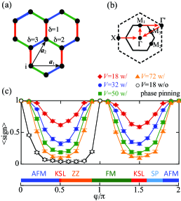
Figure 1: (a) Spin 1/2 degrees of freedom, $\hat{\boldsymbol{S}}_{\boldsymbol{i}}$, on the honeycomb lattice are subject to Heisenberg $J\hat{\boldsymbol{S}}_{i}\cdot\hat{\boldsymbol{S}}_{i+\delta}$ and Kitaev $2K\hat{S}_{i}^{\delta}\hat{S}_{i+\delta}^{\delta}$ exchange interactions. Here $\delta=1$(red), $2$(green), and $3$(blue) runs over the there bonds, and $\boldsymbol{a_{1}}$ and $\boldsymbol{a_{2}}$ correspond to the lattice vectors. (b) First (solid) and second (dashed line) Brillouin zones. (c) Average sign $\langle\text{sign}\rangle$ as a function of $V$ for various angles $\varphi$. The figure includes the ground-state phase diagram with antiferromagnetic (AFM), Kitaev spin liquid (KSL), zig-zag (ZZ), ferromagnetic (FM), and stripy (SP) phases, as proposed in Ref. [3]. Here we have set the temperature to $T=1$ in units of $A$.

Case study.— For concreteness, we consider on each $\delta$-bond, $\Gamma_{\delta}^{\alpha,\beta}=2K\delta_{\alpha,\beta}\delta_{\delta,\alpha}$ and $J_{\delta}=J$ in Eq. (1) (see Fig. 1(a)) to obtain the Kitaev-Heisenberg model:

$$\hat{H}=2K\sum_{i\in A,\delta}\hat{S}_{i}^{\delta}\hat{S}_{i+\delta}^{\delta}+J\sum_{i\in A,\boldsymbol{\delta}}\hat{\boldsymbol{S}}_{i}\cdot\hat{\boldsymbol{S}}_{i+\delta}.$$ (5)

Here $i$ runs over the A sublattice and $i+\delta$ with $\delta=(1,2,3)$ over the nearest neighbors. The first term reduces to the Kitaev model [5]. At $K=0$ the SU(2) spin symmetry of the Heisenberg model allows for sign free AFQMC simulations (see Supplemental Material). At any finite values of $K$ this symmetry is reduced to a $Z_{2}$ one in which $\boldsymbol{\boldsymbol{S}}_{\boldsymbol{i}}\rightarrow-\boldsymbol{\boldsymbol{S}}_{\boldsymbol{i}}$ and no sign free formulation is known. We used the ALF (Algorithms for Lattice Fermions) implementation [21] of the well-established finite-temperature AFQMC method [19; 34] and adopt the parametrization $K=A{\rm{sin}}(\varphi)$, $J=A{\rm{cos}}(\varphi)$, with $A=\sqrt{K^{2}+J^{2}}$. Henceforth, we use $A=1$ as the energy unit. Figure 1(c) plots the average sign as a function of the angle $\varphi$ with and without the phase pinning strategy. One observes a remarkable improvement of the average sign when the phase is pinned to $0,\pi$. A crucial question is if we can reach experimental relevant energy scales for Kitaev materials. Typical energy scales such as the charge gap $\Delta_{\rm c}$ [35] and the magnitude of the exchange interactions [9; 13] read, $(\Delta_{\rm c},A)\sim(0.35~{}\rm{eV},9~{}\rm{meV})$ for $\rm{Na}_{2}\rm{IrO}_{3}$ and $(\Delta_{\rm c},A)\sim(1.1-1.9~{}\rm{eV},4~{}\rm{meV})$ for $\alpha$-$\rm{Ru}\rm{Cl}_{3}$. As we will show below, for model parameters corresponding to the zig-zag spin ordering observed in $\alpha$-$\rm{Ru}\rm{Cl}_{3}$ we can reach temperature scales $2.6$ times lower than the exchange coupling, that is, 18K. Hence the overlap with temperature range where experimental results can be interpreted in terms of Majorana fermions, $T\in[10,100]\rm{K}$, is substantial [6; 7]. Henceforth, we will consider a $V=32$ lattice, which is beyond the accessible lattice size in exact diagonalization calculations (i.e., $V=24$ lattice) [8; 3; 9; 10; 11; 12; 13]. As for the Trotter discretization we have used a range of $\Delta\tau\in[0.01,0.1]$ depending upon the temperature. For this range of $\Delta\tau$ the systematic error is contained within our error bars. Values of $\beta U=10$ were found to be sufficient to guarantee projection to the odd parity sector.

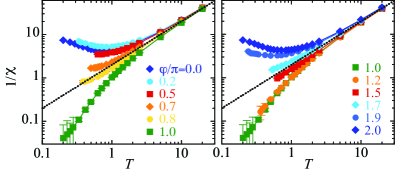
Figure 2: $T$ dependence of inverse uniform spin susceptibilities $1/\chi$ at different values of $\varphi/\pi$. Dashed line indicates the Curie’s law considered here.

The ground-state phase diagram as a function of the angle $\varphi$ presented in Ref. [3] (see Fig. 1(c)) reflects the competition between the isotropic Heisenberg exchange $J$ and the Kitaev-type bond-directional exchange $K$, and leads to antiferromagnetic (AFM), Kitaev spin liquid (KSL), zig-zag, ferromagnetic (FM), and stripy phases. To study temperature effects as a function of $\varphi$, we measure the spin susceptibility,

$$\chi_{\alpha}(\boldsymbol{q})=\int_{0}^{\beta}\text{d}\tau\langle\hat{\boldsymbol{O}}^{\alpha}_{\boldsymbol{q}}(\tau)\hat{\boldsymbol{O}}^{\alpha}_{-\boldsymbol{q}}(0)\rangle,$$

where $\hat{\boldsymbol{O}}^{\alpha}_{\boldsymbol{q}}=\frac{1}{\sqrt{V}}\sum_{\boldsymbol{r}}e^{i\boldsymbol{q}\cdot\boldsymbol{r}}\left(\hat{S}_{\boldsymbol{r},A}^{\alpha}+\hat{S}_{\boldsymbol{r},B}^{\alpha}e^{i\boldsymbol{q}\boldsymbol{R}}\right)$. Here $\boldsymbol{r}$ runs over the $A$ sublattice (or unit cell) and $\boldsymbol{R}=2/3(\boldsymbol{a_{2}}-\boldsymbol{a_{1}}/2)$.

The uniform spin susceptibility reads $\chi=\frac{1}{3}\sum_{\alpha}\chi_{\alpha}(\boldsymbol{q=\Gamma})$ and Fig. 2 plots $1/\chi$ for the various angles $\varphi$ down to the lowest accessible temperature. In the absence of sign problem at $\varphi/\pi=0$ and $1$ we can access arbitrarily low temperatures. For all values of the angle $\varphi$, $\chi$ shows a Curie law at high temperatures. The deviation from this law marks an energy scale that allows for different interpretations. One possibility is the onset of local spin correlations. In particular, in the FM case, $\varphi/\pi=1$, where $\boldsymbol{\Gamma}$ corresponds to the ordering wave vector $\chi$ grows and ultimately diverges at low temperatures. In contrast, in the AFM case, $\varphi/\pi=0$, local antiferromagnetic correlations lead to a suppression of $\chi$ with respect the high temperature Curie law. At low temperatures $\chi$ scales to a constant reflecting Goldstone modes. In the absence of ordering, especially at angles close to the Kitaev phases, the departure from the Curie law calls for different interpretations. One possibility is that frustration effects lowers the temperature scale at which local magnetic correlations develop. Other interpretations, put forward in Ref. [6], argued in terms of itinerant Majorana fermions akin to the Kitaev model [5].

Figure 3: Real-space spin-spin correlations $\langle\hat{S}^{1}_{\boldsymbol{r}}\hat{S}^{1}_{\boldsymbol{0}}\rangle$ (top panel) and momentum resolved spin susceptibility $\chi(\boldsymbol{q})=\frac{1}{3}\sum_{\alpha}\chi_{\alpha}(\boldsymbol{q})$ (bottom panel) in the first (solid) and second (dashed line) Brillouin zones (see Fig. 1(b)). (a)-(b) $\varphi/\pi=0.8$ [$T=1/2.6$], (c)-(d) $\varphi/\pi=1.7$ [$T=1/1.9$], (e)-(f) $\varphi/\pi=0.5$ [$T=1/1.6$], and (g)-(h) $\varphi/\pi=1.5$ [$T=1/1.6$].

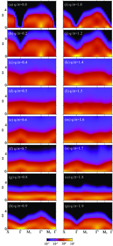
Figure 4: Dynamical spin structure factor $C(\boldsymbol{q},\omega)$ at different values of $\varphi/\pi$. Here, $T=1/1.6$. Results used here correspond to scans along the red line of Fig. 1(b).

We can confirm the above by computing real space spin-spin correlations in the zig-zag, stripy, and Kitaev phases at temperatures scales where $\chi$ departs from the Curie law. The zig-zag phase is characterized by antiferromagnerically ordered, ferromagnetic zig-zag rows of spins. This ordering is apparent in $\langle\hat{S}^{1}_{\boldsymbol{r}}\hat{S}^{1}_{\boldsymbol{0}}\rangle$ shown in Fig. 3(a). The stripy phase is characterized by antiferromagnerically ordered, ferromagnetic lines of spins. This ordering is apparent in Fig. 3(c). On the other hand, in the antiferromagnetic (Fig. 3(e)) and ferromagnetic (Fig. 3(g)) Kitaev phases, real space spin correlations are limited to the nearest neighbors. Fig. 3 equally plots the momentum resolved spin susceptibility, $\chi(\boldsymbol{q})=\frac{1}{3}\sum_{\alpha}\chi_{\alpha}(\boldsymbol{q})$. As apparent the zig-zag, Fig. 3(b), and stripy, Fig. 3(d), phases are characterized by distinct precursors of Bragg peaks. On the other hand, in the Kitaev limit only broad features are apparent around the $\boldsymbol{\Gamma}~{}(\boldsymbol{\Gamma}^{\prime}$) point for the FM (AFM) case.

We now turn our attention to the evolution of the dynamical spin structure factor as a function of angle $\varphi$ and temperature. Such calculations are of experimental relevance for the modeling of recent inelastic neutron scattering measurements [36; 7; 6]. This quantity is defined as $C(\boldsymbol{q},\omega)=\text{Im}\chi(\boldsymbol{q},\omega)/\left(1-e^{-\beta\omega}\right)$ with

$$\chi(\boldsymbol{q},\omega) =\frac{i}{3}\sum_{\gamma}\int_{0}^{\infty}dt\,e^{i\omega t}\left<\left[\hat{\boldsymbol{O}}^{\gamma}_{\boldsymbol{q}},\hat{\boldsymbol{O}}^{\gamma}_{\boldsymbol{-q}}(-t)\right]\right>.$$ (7)

We compute this quantity using the stochastic analytical continuation method [37]. In the high temperature limit where we observe a Curie law of the susceptibility ($T>10$), we expect $C(\boldsymbol{q},\omega)$ to show no momentum dependence, and spectral weight centered around $\omega\sim 0$. Data at $T=10$ is shown in the Supplemental Material. At $T=1/1.6$ Fig. 4 shows that the angle dependence of $C(\boldsymbol{q},\omega)$ is pronounced and that the distinct features of the ordered and disordered phases are apparent. For the KSL at $\varphi/\pi=0.5$, we see intensity located along the $\boldsymbol{\rm M_{1}}-\boldsymbol{\rm M_{3}}$ line as well as around the $\boldsymbol{\rm X}$ point. In contrast, strong intensity around the $\boldsymbol{\Gamma}$ point is apparent in the FM case ($\varphi/\pi=1.5$). Similar behavior has been reported for the Kitaev model [38] below a temperature scale related the coherence scale of the Majorana fermions [39]. In the Heisenberg limits, our data produce the well-known features of the spin-wave dispersion relation: a quadratic dispersion around $\boldsymbol{\Gamma}$ the FM case ($\varphi/\pi=1$), and a linear one around $\boldsymbol{\Gamma}^{\prime}$ for the AFM ($\varphi/\pi=0$). Moving away form the AFM or FM phase towards the KSLs (Fig. 4(a)-(d) and (i)-(l)) our data shows the progressive vanishing of the spin wave features. At $\varphi/\pi=0.7$ we observe a buildup of low-lying spectral weight at the $\boldsymbol{\rm M_{1}}$ and $\boldsymbol{\rm M_{3}}$ points as appropriate for the zig-zag ordering. In contrast in the stripy phase at $\varphi/\pi=1.7$ we observe substantial low-lying weight at the $\boldsymbol{\rm X}$ and $\boldsymbol{\Gamma}^{\prime}$ points. Note that this data is taken at higher temperatures than the susceptibility results of Fig. 3 (c) and (d) and that $\varphi/\pi=1.7$ is close to the AFM phase. We understand the low-lying weight at $\boldsymbol{\Gamma^{\prime}}$ as a combined effect of temperature and proximity to the AFM phase. It is interesting to consider the temperature dependence of the zig-zag phase proximate to the KSL at $\varphi/\pi=0.8$. As a function of decreasing temperature, Figs. 5(a), 4(g) and 5(b) we first observe a buildup of weight around the $\boldsymbol{\Gamma}$ point followed by a softening at $\boldsymbol{\rm M_{1}}$ and $\boldsymbol{\rm M_{3}}$. The low temperature dynamical spin structure factor with high (low) energy weight at $\boldsymbol{\Gamma}$ ($\boldsymbol{\rm M_{1}}$ and $\boldsymbol{\rm M_{3}}$) bears similarities to inelastic neutron scattering experiments for $\alpha$-RuCl₃ reported in [7; 6].

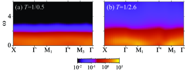
Figure 5: Dynamical spin structure factor $C(\boldsymbol{q},\omega)$ at $\varphi/\pi=0.8$ for higher [(a)$T=1/0.5$] and lower [(b)$T=1/2.6$] temperatures.

Summary and discussion.— We have defined a formulation of the auxiliary field QMC algorithm for the generalized Kitaev model of Eq. (1) in which the imaginary part of the action is pinned by symmetry to $0$ or $\pi$. It turns out that this phase pinning strategy greatly improves the negative sign problem and opens a window of temperatures relevant to experiments where simulations can be carried out. We demonstrate this by carrying out extensive simulations of thermodynamical and dynamical properties of the Kitaev-Heisenberg model. Aside from the magnetic susceptibility and dynamical spin structure factor presented in this Letter, we can compute the specific heat, the magnetotropic coefficient  [40] as well as heat transport [41]. Furthermore our numerical method for the generalized Kitaev model of Eq. (1) can be applied to longer ranged interactions as well as off-diagonal $\Gamma^{\alpha,\beta}$ interactions regarding specific materials such as $\rm{Na}_{2}\rm{IrO}_{3}$ and $\alpha$-$\rm{Ru}\rm{Cl}_{3}$. Comparison of the aforementioned quantities with experimental data over a wide temperature range provides a useful tool to determine model parameters.

I Supplemental Material

In this supplemental material section we will first provide a demonstration of the phase pinning approach and then show how to implement this idea for the general Hamiltonian of Eq. (1) of the main text. Next, we will plot the uniform susceptibility data presented in the main text on a linear scale so as to emphasis the Curie-Weiss behavior. We will then provide further data for the spin-spin correlations in the zig-zag and stripy phases of the Kitaev-Heisenberg model of Eq. (5) of the main text. Finally we will discuss the dynamical spin structure factor at higher temperatures than considered in the main text for the Kitaev-Heisenberg model of Eq. (5) of the main text.

I.1 The phase pinning approach

Consider the action:

$$S(\Phi)=S_{0}(\Phi)-\log\text{Tr}\left[{\cal T}e^{-\int_{0}^{\beta}d\tau\hat{\boldsymbol{c}}^{\dagger}h(\tau)\hat{\boldsymbol{c}}^{\phantom{\dagger}}}\right]$$ (8)

with

$$\sum_{x,y}\hat{c}^{\dagger}_{x}h_{x,y}(\tau)\hat{c}^{\phantom{\dagger}}_{y}=\hat{\boldsymbol{c}}^{\dagger}h(\tau)\hat{\boldsymbol{c}}^{\phantom{\dagger}}.$$ (9)

Here, $x$, $y$ run over the single particle states.

We will assume that we can find an anti-unitary operator:

$$\hat{T}=\hat{K}\hat{U}$$ (10)

that commutes with the single body Hamiltonian:

$$\left[\hat{\boldsymbol{c}}^{\dagger}h(\tau)\hat{\boldsymbol{c}}^{\phantom{\dagger}},\hat{T}\right]=0\,\,\,\forall\,\,\,\tau.$$ (11)

Here $\hat{U}$ is unitary and $\hat{K}$ corresponds to complex conjugation.

Equation (11) is equivalent to:

$$\hat{U}^{\dagger}\hat{\boldsymbol{c}}^{\dagger}\hat{U}^{\phantom{\dagger}}\overline{h}(\tau)\hat{U}^{\dagger}\hat{\boldsymbol{c}}^{\phantom{\dagger}}\hat{U}^{\phantom{\dagger}}=\hat{\boldsymbol{c}}^{\dagger}h(\tau)\hat{\boldsymbol{c}}^{\phantom{\dagger}}$$ (12)

where $\overline{h}(\tau)$ denotes the element wise complex conjugation of the matrix $h(\tau)$. Thereby:

$$\overline{\text{Tr}\left[{\cal T}e^{-\int_{0}^{\beta}d\tau\hat{\boldsymbol{c}}^{\dagger}h(\tau)\hat{\boldsymbol{c}}^{\phantom{\dagger}}}\right]}=\text{Tr}\left[{\cal T}e^{-\int_{0}^{\beta}d\tau\hat{\boldsymbol{c}}^{\dagger}\overline{h(\tau)}\hat{\boldsymbol{c}}^{\phantom{\dagger}}}\right]=$$ (13)

$$\text{Tr}\left[{\cal T}e^{-\int_{0}^{\beta}d\tau\hat{U}^{\dagger}\hat{\boldsymbol{c}}^{\dagger}\hat{U}^{\phantom{\dagger}}\overline{h(\tau)}\hat{U}^{\dagger}\hat{\boldsymbol{c}}^{\phantom{\dagger}}\hat{U}^{\phantom{\dagger}}}\right]=\text{Tr}\left[{\cal T}e^{-\int_{0}^{\beta}d\tau\hat{\boldsymbol{c}}^{\dagger}h(\tau)\hat{\boldsymbol{c}}^{\phantom{\dagger}}}\right].$$

In the above, $\hat{U}^{\dagger}\hat{\boldsymbol{c}}^{\phantom{\dagger}}\hat{U}^{\phantom{\dagger}}$ corresponds to a canonical transformation of the $\hat{\boldsymbol{c}}^{\phantom{\dagger}}$ fermion operator such that the trace remains invariant. Hence, $\text{Tr}\left[{\cal T}e^{-\int_{0}^{\beta}d\tau\hat{\boldsymbol{c}}^{\dagger}h(\tau)\hat{\boldsymbol{c}}^{\phantom{\dagger}}}\right]$ is real and

$$\text{Im}S=0,\pi.$$ (14)

I.2 Optimal AFQMC formulation of the generalized Kitaev model

Here we show that we can apply the phase pinning method to the generalized Kitaev model of Eq. (1) of the main text. We start by adopting a fermion representation of the spin-1/2 degree of freedom: $\hat{\boldsymbol{S}}_{i}=\frac{1}{2}\hat{\boldsymbol{f}}^{\dagger}_{i}\hat{\boldsymbol{\sigma}}\hat{\boldsymbol{f}}^{\phantom{\dagger}}_{i}$ where $\hat{\boldsymbol{f}}^{\dagger}_{i}\equiv\left(\hat{f}^{\dagger}_{i,\uparrow},\hat{f}^{\dagger}_{i,\downarrow}\right)$ is a two-component fermion with constraint $\hat{\boldsymbol{f}}^{\dagger}_{i}\hat{\boldsymbol{f}}^{\phantom{\dagger}}_{i}=1$. Let us now relax the constraint on the Hilbert space, and enforce by adding a Hubbard $U$ term on each site. The Hamiltonian that we will simulate reads:

$$\hat{H}_{{\rm QMC}} = \sum_{i,j,\alpha,\beta}\frac{|\Gamma_{i,j}^{\alpha,\beta}|}{2}\left(\hat{S}_{i}^{\alpha}+\frac{\Gamma_{i,j}^{\alpha,\beta}}{|\Gamma_{i,j}^{\alpha,\beta}|}\hat{S}_{j}^{\beta}\right)^{2}$$ (15)

$$-\sum_{i,j}\frac{J_{i,j}}{8}\left(\left(\hat{D}^{\dagger}_{i,j}+\hat{D}^{\phantom{\dagger}}_{i,j}\right)^{2}+\left(i\hat{D}^{\dagger}_{i,j}-i\hat{D}^{\phantom{\dagger}}_{i,j}\right)^{2}\right)$$

$$+U\sum_{i}\left(\hat{\boldsymbol{f}}^{\dagger}_{i}\hat{\boldsymbol{f}}^{\phantom{\dagger}}_{i}-1\right)^{2},$$

where $\hat{D}^{\dagger}_{i,j}=\hat{\boldsymbol{f}}^{\dagger}_{i}\hat{\boldsymbol{f}}^{\phantom{\dagger}}_{j}$. It is important to note that $\left[\left(\hat{\boldsymbol{f}}^{\dagger}_{i}\hat{\boldsymbol{f}}^{\phantom{\dagger}}_{i}-1\right)^{2},\hat{H}_{\rm{QMC}}\right]=0$ such that the $\hat{\boldsymbol{f}}$-fermion parity $(-1)^{\hat{\boldsymbol{f}}^{\dagger}_{i}\hat{\boldsymbol{f}}^{\phantom{\dagger}}_{i}}$ is a local conserved quantity and that the constraint is very efficiently imposed. We will discuss this point at the end of the section. In the odd parity sector favored by the repulsive Hubbard interaction, $\left.\hat{H}_{\rm{QMC}}\right|_{(-1)^{\hat{\boldsymbol{f}}^{\dagger}_{i}\hat{\boldsymbol{f}}^{\phantom{\dagger}}_{i}}=-1}=\hat{H}+C$ where $C$ is a constant.

The above form in terms of perfect squares can be implemented in the ALF-implementation of the auxiliary field QMC (AFQMC) algorithm. As mentioned in the main text, the $J_{i,j}$ exchange constants are non-frustrating. This means that we can find a set of Ising spins, $s_{i}=\pm 1$, such that for each bond with $J_{i,j}\neq 0$, $J_{i,j}s_{i}s_{j}<0$. Hence,

$$J_{i,j}=|J_{i,j}|\left(-s_{i}s_{j}\right).$$ (16)

After Trotter decomposition and Hubbard-Stratonovich transformation the grand canonical partition function reads:

$$Z= {\rm{Tr}}\left[e^{-\beta\hat{H}_{\rm{QMC}}}\right]\propto$$ (17)

$$\int D\left\{\chi_{i,j}^{\alpha,\beta}(\tau),{\rm{Re}}Z_{i,j}(\tau),{\rm{Im}}Z_{i,j}(\tau),\lambda_{i}(\tau)\right\}$$

$$\times e^{-S\left(\left\{\chi_{i,j}^{\alpha,\beta}(\tau),Z_{i,j}(\tau),\lambda_{i}(\tau)\right\}\right)}.$$

For given field configuration, $\chi_{i,j}^{\alpha,\beta}(\tau),\lambda_{i}(\tau)\in\mathbb{R}$ and $Z_{i,j}(\tau)\in\mathbb{C}$, the action is given by:

$$S\left(\left\{\chi,Z,\lambda\right\}\right)= \int_{0}^{\beta}d\tau\left[\sum_{i,j,\alpha,\beta}\frac{\left(\chi_{i,j}^{\alpha,\beta}(\tau)\right)^{2}}{|\Gamma_{i,j}^{\alpha,\beta}|}\right.$$ (18)

$$\left.+\sum_{i,j}\frac{|Z_{i,j}(\tau)|^{2}}{4|J_{i,j}|}+\sum_{i}\frac{\lambda_{i}(\tau)^{2}}{2U}\right]$$

$$-\ln{\rm{Tr}}{\cal T}e^{-\int_{0}^{\beta}d\tau\hat{H}(\left\{\chi,Z,\lambda\right\})}$$

with

$$\hat{H}(\left\{\chi,Z,\lambda\right\}) = \sum_{i,j,\alpha,\beta}i\chi_{i,j}^{\alpha,\beta}(\tau)\left(\hat{S}_{i}^{\alpha}+\frac{\Gamma_{i,j}^{\alpha,\beta}}{|\Gamma_{i,j}^{\alpha,\beta}|}\hat{S}_{j}^{\beta}\right)$$ (19)

$$+\sum_{i,j\delta}\sqrt{-s_{i}s_{j}}\left(Z_{i,j}(\tau)\hat{D}^{\dagger}_{i,j}+\overline{Z_{i,j}(\tau)}\hat{D}^{\phantom{\dagger}}_{i,j}\right)$$

$$+\sum_{i}i\lambda_{i}(\tau)\left(\hat{\boldsymbol{f}}^{\dagger}_{i}\hat{\boldsymbol{f}}^{\phantom{\dagger}}_{i}-1\right).$$

In the above, it is understood that the first sum runs over bonds and spin indices where $\Gamma_{i,j}^{\alpha,\beta}\neq 0$. Similarly the second sum runs over bonds where $J_{i,j}$ does not vanish. Now consider the anti-unitary transformation

$$\hat{T}\alpha\hat{f}^{\dagger}_{\boldsymbol{i},\sigma}\hat{T}^{-1}=\overline{\alpha}s_{i}\hat{f}^{\phantom{\dagger}}_{\boldsymbol{i},\sigma}$$ (20)

where $\alpha$ is a complex number. One will show that

$$\hat{T}\hat{H}(\left\{\chi,Z,\lambda\right\})\hat{T}^{-1}=\hat{H}(\left\{\chi,Z,\lambda\right\})$$ (21)

such that for this formulation

$${\rm{Im}}S\left(\left\{\chi,Z,\lambda\right\}\right)=0,\pi.$$ (22)

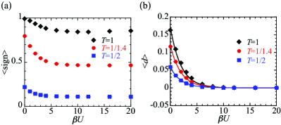
Figure 6: $\beta U$ dependence of (a) average sign $\langle\text{sign}\rangle$ and (b) double occupancy $d=\langle\hat{f}^{\dagger}_{i,\uparrow}\hat{f}_{i,\uparrow}\hat{f}^{\dagger}_{i,\downarrow}\hat{f}_{i,\downarrow}\rangle$ for different temperatures $T=1/\beta$. Here, $\varphi/\pi=0.2$ (see text) and lattice size $V=32$. The solid lines in (b) are the results of the fitting Eq.(23).

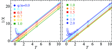
Figure 7: $T$ dependence of inverse uniform spin susceptibilities $1/\chi$ at different values of $\varphi/\pi$. The solid lines are a fit to Curie-Weiss law in the range $T\in[5,10]$.

We note that when the generalized Kitaev term is set to zero, the action for each field configuration, and the model, have an additional SU(2) spin symmetry. This implies that the fermion determinant factorizes in up and down spin sectors. Owing to the SU(2) spin symmetry the fermion determinants are identical in each spin sector. The anti-unitary transformation of Eq. (20) can be applied in each spin sector to show that the fermion determinant is real. Hence in this case, there is no sign problem since the weight is given by the square of a real number.

We conclude this section by discussing the convergence to the physical Hilbert space. Since, as mentioned above, $\left[\left(\hat{\boldsymbol{f}}^{\dagger}_{i}\hat{\boldsymbol{f}}^{\phantom{\dagger}}_{i}-1\right)^{2},\hat{H}_{\rm{QMC}}\right]=0$ one can show that

$$\left<\left(\hat{\boldsymbol{f}}^{\dagger}_{i}\hat{\boldsymbol{f}}^{\phantom{\dagger}}_{i}-1\right)^{2}\right>\propto e^{-\beta U/2}.$$ (23)

Owing to the invariance of the action under the particle-hole symmetry of Eq. (20), $\left<\hat{\boldsymbol{f}}^{\dagger}_{i}\hat{\boldsymbol{f}}^{\phantom{\dagger}}_{i}\right>=1$ such that

$$\left<\left(\hat{\boldsymbol{f}}^{\dagger}_{i}\hat{\boldsymbol{f}}^{\phantom{\dagger}}_{i}-1\right)^{2}\right>=2\langle\hat{f}^{\dagger}_{i,\uparrow}\hat{f}_{i,\uparrow}\hat{f}^{\dagger}_{i,\downarrow}\hat{f}_{i,\downarrow}\rangle.$$ (24)

The double occupancy is plotted in Fig. 6 (b) and as apparent follows the predicted exponential form. Clearly values of $\beta U=10$ suffice to guarantee convergence to the physical Hilbert space. It is vey interesting to consider the average sign as a function of $\beta U$. Generically, the sign decays exponentially with inverse temperature. In contrast to this general expectation, Fig. 6 (a), shows that the average sign converges to a constant.

Figure 8: Real-space spin-spin correlations $\langle\hat{S}^{\alpha}_{\boldsymbol{r}}\hat{S}^{\alpha}_{\boldsymbol{0}}\rangle$ (top panel) and momentum resolved spin susceptibility $\chi_{\alpha}(\boldsymbol{q})$ (bottom panel) in the first (solid) and second (dashed line) Brillouin zones. Here we consider $\varphi/\pi=0.8$ and $T=1/2.6$. (a)-(b) $\alpha=1$, (c)-(d) $\alpha=2$, and (e)-(f) $\alpha=3$.

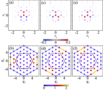
Figure 9: Real-space spin-spin correlations $\langle\hat{S}^{\alpha}_{\boldsymbol{r}}\hat{S}^{\alpha}_{\boldsymbol{0}}\rangle$ (top panel) and momentum resolved spin susceptibility $\chi_{\alpha}(\boldsymbol{q})$ (bottom panel) in the first (solid) and second (dashed line) Brillouin zones. Here we consider $\varphi/\pi=1.7$ and $T=1/1.9$. (a)-(b) $\alpha=1$, (c)-(d) $\alpha=2$, and (e)-(f) $\alpha=3$.

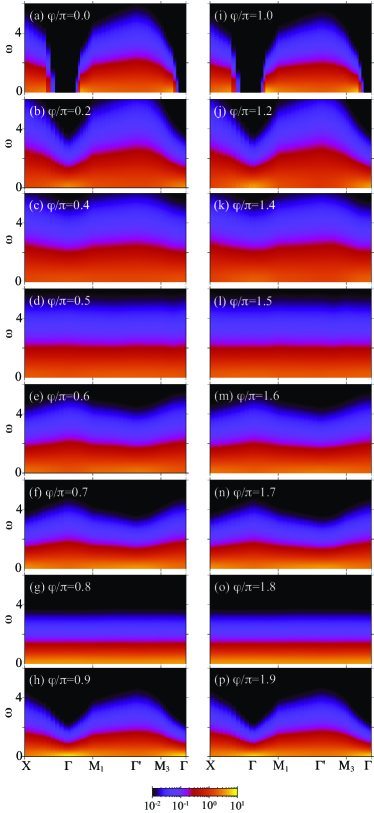
Figure 10: Dynamical spin structure factor $C(\boldsymbol{q},\omega)$ at different values of $\varphi/\pi$. Here, $T=10$. Results used here correspond to scans along the red line of Fig. 1(b) of the main text.

I.3 Curie-Weiss behaviors

In the main text our QMC results for the uniform spin susceptibilities $\chi$ as a function of the angle $\varphi$ and temperature support the departure from the high-temperature Curie law in the ordered and disordered phases inherent to the Kitaev-Heisenberg model of Eq. (5) of the main text. At very high temperatures local correlations are impaired so that the Curie law is obeyed. With decreasing temperatures local correlations develop and one can expect the Curie law to give way to Curie-Weiss one, at least in an intermediate temperature range. In Fig. 7, we plot our inverse susceptibility data, $1/\chi$, presented in the main text on a linear scale. For all values of $\varphi$, $1/\chi$ indeed follows the predicted Curie-Weiss form $1/\chi=(T-\Theta_{\rm cw})/C$ in an intermediate temperature range. Note that as a function of $\varphi$ the sign of the Curie-Weiss temperature $\Theta_{\rm cw}$ changes from negative to positive reflecting the sign of the dominant local exchange coupling.

I.4 Spin correlations in the zig-zag and stripy phases

The Kitaev-Heisenberg model of Eq. (5) of the main text remains invariant under combined $2\pi/3$ rotations and a permutation of the elements of the spin vector $\left(\hat{S}^{1}_{\boldsymbol{r}},\hat{S}^{2}_{\boldsymbol{r}},\hat{S}^{3}_{\boldsymbol{r}}\right)$. As a consequence the ordering pattern in the zig-zag (Fig. 8) and stripy (Fig. 9) phases, rotate by a $2\pi/3$ angle when measuring for instance $\langle\hat{S}^{2}_{\boldsymbol{r}}\hat{S}^{2}_{\boldsymbol{0}}\rangle$ instead of $\langle\hat{S}^{1}_{\boldsymbol{r}}\hat{S}^{1}_{\boldsymbol{0}}\rangle$. Figures 8 and 9 confirm this, thus providing a benchmark for our code.

I.5 High-temperature spin dynamics

In order to capture finite temperature properties of ordered and spin-liquid ground states inherent to the Kitaev-Heisenberg model of Eq. (5) of the main text, we computed the dynamical spin structure factor at different temperatures. In our QMC simulations, the dynamical spin structure factor $C(\boldsymbol{q},\omega)$ of Eq. (7) of the main text is obtained via the analytic continuation of the imaginary-time-displaced spin correlation functions. We used the Algorithms for Lattice Fermions (ALF) [21] implementation of the stochastic analytical continuation [37].

In the main text we show that $C(\boldsymbol{q},\omega)$ at $T=1/1.6$ and as a function of $\varphi$ picks up the distinct finite temperature features of the ordered and disordered phases of the Kitaev-Heisenberg model. As the temperature increases, local correlations are impaired so that $C(\boldsymbol{q},\omega)$ is expected to become ${\boldsymbol{q}}$-independent with spectral weight centered around low frequencies. Figure 10 shows results at higher temperatures, $T=10$. Consider $\varphi/\pi=0.8$ corresponding to the zig-zag phase. Comparison of the high temperature data in Fig. 10 with that of the lower temperature data in Fig. 5 of the main text shows spectral weight shifting for low to high energies and the emergence of distinct $\boldsymbol{q}$ dependence. Note that the angles $\varphi/\pi=0,1$ stand apart due to the enhanced SU(2) spin symmetry. For these angles the total spin is a conserved quantity such that the dynamical spin structure factor at the $\boldsymbol{\Gamma}$ point and at any temperature is given by a Dirac $\delta$-function in frequency.