Digital Annealer for quadratic unconstrained binary optimization: a comparative performance analysis
Abstract
Digital Annealer (DA) is a computer architecture designed for tackling combinatorial optimization problems formulated as quadratic unconstrained binary optimization (QUBO) models. In this paper, we present the results of an extensive computational study to evaluate the performance of DA in a systematic way in comparison to multiple state-of-the-art solvers for different problem classes. We examine pure QUBO models, as well as QUBO reformulations of three constrained problems, namely quadratic assignment, quadratic cycle partition, and selective graph coloring, with the last two being new applications for DA. For the selective graph coloring problem, we also present a size reduction heuristic that significantly increases the number of eligible instances for DA. Our experimental results show that despite being in its development stage, DA can provide high-quality solutions quickly and in that regard rivals the state of the art, particularly for large instances. Moreover, as opposed to established solvers, within its limit on the number of decision variables, DA’s solution times are not affected by the increase in instance size. These findings illustrate that DA has the potential to become a successful technology in tackling combinatorial optimization problems.
keywords:
Quadratic unconstrained binary optimization; Digital Annealer; combinatorial optimization; computational testing; quadratic cycle partition; selective graph coloring1 Introduction
Combinatorial optimization problems (COPs) aim to choose the best solution among a finite set of possible solutions in terms of a given objective function. They constitute an important problem class having diverse applications, such as in scheduling, resource allocation, production planning, transportation, telecommunications and network design (Paschos 2013). As such, there is a vast literature on solution methods for these optimization problems, which can be classified as general-purpose methods and problem-specific methods, or, as exact methods and heuristics. In this paper, we focus on an emerging general heuristic approach to solving COPs. More specifically, we employ the Digital Annealer, a hardware architecture specially designed for solving COPs, using the so-called Ising formulations, to generate high-speed and high-quality solutions. We conduct a computational study to assess the performance of this recent approach compared to traditional ones. In addition, we provide two new applications for this promising technology. In what follows, we first review the solution methods for COPs and the literature on the Digital Annealer, then provide the details of our study.
1.1 Solution methods for COPs
General-purpose methods are designed to be adapted to every COP. The most commonly used approach is to formulate the problem as an integer program (IP), and solve it (exactly) via a state-of-the-art solver, e.g., GUROBI (Gurobi Optimization 2018), CPLEX (CPLEX 2009) and SCIP (Achterberg 2009). The IP solvers are powerful in the sense that they can usually find optimal solutions to moderate-size COPs in a reasonable amount of time. However, in large-scale problems, more specifically real industrial problems, IP solvers are unable to provide even good quality solutions, let alone optimal ones, quickly. This may happen due to the complexity of the problem at hand, time limitation to provide a solution, and size of the instances. This brings the necessity of developing general-purpose heuristic methods. Moreover, as also mentioned in (Giovanni 2017), in many large-scale cases including most real-life applications, it is sufficient to obtain a good-quality solution. In practice, it is mostly desired to find high-quality feasible solutions in a short amount to be implemented in real time. Other than the need of obtaining solutions for a dynamic decision-making framework, fast generation of feasible solutions can be useful to evaluate potential future scenarios for the system and pick the best one to be implemented. Lastly, the extra effort of finding an optimal solution may not be worthwhile due to potential estimation errors in many problem parameters. In order to produce good-quality solutions for large-scale COPs, many heuristics (Gillett and Miller 1974; Gupta 1971; Nawaz, Enscore Jr, and Ham 1983) and meta-heuristics (Kaveh 2014; Lee and Geem 2005; Qiao and Yang 2019), specifically the ones based on simulated annealing (Bandyopadhyay et al. 2008; Suman 2004; Van Breedam 1995), are proposed in the literature.
There are problem-specific methods developed to address particular families of COPs. For instance, the shortest path problem is one of the famous COPs for which efficient (exact) solution methods are proposed, e.g., the Dijkstra’s algorithm (Delling et al. 2009; Dijkstra 1959) and label correcting algorithms (Bertsekas 1993). Such methods are very powerful in the sense that they can provide high-quality solutions for large-scale problems in a short amount of time. However, problem-specific methods exist only for a small portion of COPs.
A recently arising theme in the literature is to formulate a COP as a quadratic unconstrained binary optimization (QUBO) model (Glover, Kochenberger, and Du 2018) and employ a specialized hardware to solve it. The goal is to propose a general methodology in order to tackle COPs and provide high-quality solutions very quickly, e.g., in a matter of minutes. Although COPs are usually modeled as constrained binary linear programs, solving their QUBO reformulations via a hardware specially designed for QUBOs with the aforementioned aim can indeed outperform solving their natural formulations via an IP solver. Moreover, QUBO problems naturally arise in many applications such as routing (Irie et al. 2019; Papalitsas et al. 2019), scheduling (Tran et al. 2016; Venturelli, Marchand, and Rojo 2015), finance (Elsokkary et al. 2017; Orus, Mugel, and Lizaso 2019), and biology (Li et al. 2018; Oliveira, Silva, and Oliveira 2018). These problems are more challenging, thus amenable to these new technologies.
Moore’s law was the golden rule that set the pace for modern digital revolution for the last fifty years. By approaching to the end of this era, it became clear that the traditional silicon-based processors cannot effort the current computational burden. Therefore, there is need for new technologies which can handle optimization problems using reasonable time and energy. Based on these observations, new architecture designs have been making a frequent appearance in the digital industry. One of the recent developments is the introduction of quantum annealing-based hardware which is commercialized by D-Wave Systems Inc. Although it is guaranteed that quantum annealing provides high-quality solutions under ideal conditions, this technology in its current development stage can be very expensive and difficult to run (Sao et al. 2019). In order to overcome the disadvantages of quantum annealing-based hardware, Fujitsu designed and developed a new computer architecture implemented in digital circuit, the Digital Annealer (DA), to address complex COPs efficiently (Matsubara et al. 2020).
A natural way to use a QUBO approach in solving COPs is to formulate the entire problem under consideration as a QUBO model, and feed it to a solver capable of tackling such models, a promising example to which is the DA. One can also utilize QUBO modeling approach at different levels of a solution strategy. For the quadratic assignment problem for instance, Liu et al. (2019) present a local search based iterative method, which is an extension of the so-called quantum local search (QLS) algorithm. While in QLS a QUBO model is constructed for a single subset of selected variables at each step of the local search to find an improving solution, the authors extend it by choosing multiple subsets of variables and solving a separate QUBO model for each at every step. Other problems addressed in a similar manner include graph partitioning and network community detection problems (Shaydulin et al. 2019, 2019; Ushijima-Mwesigwa et al. 2020). Our QUBO approach in this work is to reformulate the full binary constrained formulations of the problems as QUBO models and solving them with DA and selected established solvers.
1.2 Applications of DA
In this section, we briefly review some works from the literature that focus on the use of DA in different application areas. Aramon et al. (2019) use DA to solve the so-called spin-glass problem in physics, where the problem is formulated as an Ising model and performance of DA is compared with the simulated annealing and parallel tempering Monte Carlo methods. The results show that DA is orders of magnitude faster than the other two methods in solving fully connected spin-glass problems; however, it fails to achieve a speedup for sparse two-dimensional spin-glass problems.
Rahman et al. (2019) consider the outlier rejection problem in the context of WiFi-based positioning and represent it as a QUBO model. They show that solving the problem with DA significantly improves localization accuracy when compared to state-of-the-art methods. Graph problems comprise another application area that has been addressed using DA. Javad-Kalbasi et al. (2019) use DA in order to a solve sensor placement problem by modeling it as a minimum vertex cover problem, and report that DA is able to find optimal solutions to all tested benchmark instances and delivers high-quality solutions for a large suite of randomly generated graphs in comparison to well-known alternatives from the literature. Another such study is by Naghsh, Javad-Kalbasi, and Valaee (2019), in which the authors consider the maximum weighted clique problem on both benchmark and randomly generated instances and report that DA outperforms various existing algorithms as well as the state-of-the-art solver CPLEX.
A real-life application of DA is proposed by Ohzeki et al. (2019), where the problem of controlling a large number of automated guided vehicles in a factory in Japan is formulated as a QUBO model. The authors solve the resulting QUBO formulation using D-Wave, DA and GUROBI, and compare their results. By comparing current versions of D-Wave and DA, they show that the probability of attaining an optimal solution using DA is much higher than that of D-Wave, and that DA can solve the considered problem instances without any need to divide the original problem into smaller subproblems.
DA is also used to handle a machine learning problem. Salehinejad and Valaee (2019) propose a novel regularization method based on an Ising model for the training phase of a deep neural network. One of the recent works focusing on applications and performance analysis of DA is by Matsubara et al. (2020), which evaluates the efficiency of DA on the maximum/minimum cut problem and the quadratic assignment problem in comparison to CPLEX. The authors report that DA outperforms CPLEX in terms of computation time and solution quality. Another recent work is by Şeker, Bodur, and Pouya (2020), where the authors address a routing and wavelength assignment problem with a QUBO approach, and show that solving it using DA outperforms or is comparable to established techniques coupled with the state-of-the-art solvers.
1.3 Our contributions
In this paper, we present the results of an extensive computational study to assess the quality of solutions that DA yields, which, to the best of our knowledge, has not been analyzed in detail in the literature. We first consider problems that are originally formulated as QUBO models. We conduct experiments on a large set of instances from existing QUBO libraries, comparing the performance of DA with three state-of-the-art exact solvers. In addition, we analyze the impact of variable ordering on the obtained solution quality for DA.
In order to develop a better understanding of DA’s efficiency in different classes of problems, we also consider problems whose natural formulations include constraints, and conduct performance analyses for solving their QUBO reformulations. In that regard, we use the quadratic assignment problem (QAP) since it also has available benchmark instances. Moreover, we introduce two new applications for DA, the quadratic cycle partition problem (QCPP), and the selective graph coloring problem (Sel-Col), which is a generalization of the classical graph coloring problem. For Sel-Col, we design a heuristic method that significantly reduces problem size, hence greatly increasing the number of instances that can be solved by DA.
Our contributions are as follows:
-
1.
To the best of our knowledge, our study constitutes the first work assessing the performance of DA in a systematic way, in comparison to multiple state-of-the-art exact solvers for different problem classes. Our experiments show that despite being in its development stage, DA can provide high-quality solutions quickly, which, combined with the fact that the next generation of DA will allow up to one million binary variables (Fujitsu Limited 2020), indicates DA has the potential to become a successful technology in tackling large-scale COPs.
-
2.
We find that DA outperforms the state of the art typically in large instances and is usually comparable otherwise, and illustrate that its performance is robust to the increase in the number of decision variables or constraints, as opposed to established solvers whose performance is known to be significantly sensitive to both.
-
3.
We introduce two new applications for DA, namely QCPP and Sel-Col, and demonstrate that DA is particularly successful in yielding better solutions for instances that are challenging for the state-of-the-art solvers. Moreover, we apply a size reduction heuristic for Sel-Col that makes a significantly larger number of instances eligible for DA.
-
4.
We analyze the effect of variable ordering and penalty coefficient values on the performance of DA, and show that they might need to be carefully selected in certain cases to increase the obtained solution quality.
The remainder of this paper is organized as follows. In Section 2, we overview our solution approaches and the operating principles of state-of-the-art exact solvers and DA. In Section 3, we analyze the performance of the solvers and DA on the four problem classes we consider. Finally, we provide conclusions and future research directions in Section 4.
2 Solution approaches
In this section, we briefly explain the basic modeling and algorithmic principles behind three general methods to solve a COP, namely (i) solving an IP formulation of the problem via an exact solver, (ii) solving a QUBO formulation of the problem via an exact solver, and (iii) solving the QUBO formulation via DA.
2.1 IP approach
In general, any COP can be formulated as a binary linear program:
| (1a) | ||||
| s.t. | (1b) | |||
| (1c) | ||||
where , and . In other words, the goal is to find a solution which minimizes the linear objective function (1a), and satisfies all of the linear constraints (1b) as well as variable domain restrictions (1c).
State-of-the-art solvers such as GUROBI and CPLEX employ a linear programming-based branch-and-bound (BB) algorithm to solve binary linear programs. This algorithm conducts the search of an optimal solution in a structured way, specifically in the form of a search tree. At the root node of the tree, it solves the so-called linear programming relaxation of the model (1) obtained by relaxing all integrality conditions on the decision variables, (1c). This yields a lower bound on the optimal value of the COP. If the obtained solution at the root node is not binary, the algorithm splits the search space (i.e., the relaxed feasible region) into smaller subregions based on branching rules, each excluding the infeasible relaxation solution. Creating one node per subregion in the search tree, the algorithm continues the search by repeating this procedure. Each node in the search tree represents the linear programming relaxation of model (1) with additional constraints defining the subregion specific to that node. If the solution at a node is binary, then it is a feasible solution for the original binary linear program, the associated objective value constitutes an upper bound for the optimal objective value, and there is no need to further branch on that node. Otherwise, i.e., if there is a non-binary value in the solution, the algorithm decides on whether to further branch on that node by comparing the objective value of the node to the best upper bound found so far. If the objective value is at least as large as the best upper bound, the algorithm discards that node because it cannot produce a better solution than the best one found so far. In this manner, the BB algorithm avoids unnecessary computations in the search process. Choosing well-suited branching rules and effective bounding techniques are two major considerations in the use of BB algorithms, which significantly impact the size of the search tree, thus the solution time. In addition to employing multiple carefully designed branching and bounding rules, the state-of-the-art solvers also implement a variety of enhancement techniques to improve the BB performance, including presolve methods to reduce the size of the models, cutting planes to strengthen the relaxations, and heuristics to discover good quality solutions during the search. For more information about recent developments on the BB algorithm, we refer the reader to (Morrison et al. 2016).
It is also possible to incorporate a quadratic component in the objective function for certain problems, in which case model (1) can be generalized into the following:
| (2a) | ||||
| s.t. | (2b) | |||
| (2c) | ||||
where and symmetric. Whether the objective function is linear or quadratic, we refer to models as in (1) and (2) as IP models in this study, and call the approach of handling such models as the IP approach.
In order to solve binary quadratic problems, exact and heuristic methods exist in the literature. Initially proposed exact methods are (general) BB-based algorithms. In this regard, effective methods to make a quadratic model compatible with the BB framework and useful bounding techniques have been developed. Linearization methods aim to introduce a full linear representation of the quadratic model and tackle the problem using exact IP solvers and algorithms. This method requires the addition of new decision variables and constraints to the model, which in most cases increases the size of the problem significantly. On the other hand, outer approximation techniques try to approximate the objective function using supporting hyperplanes. They have been shown to be efficient for certain quadratic optimization problems, when supporting hyperplanes are easy to generate. Exact solvers handle such models typically by benefiting from linearization and outer approximation techniques as well as other ideas used in treating nonlinear programs (Furini and Traversi 2013; Achterberg and Towle 1998).
There exist advanced solvers that can solve certain types of quadratic models exactly. A mixed-integer quadratic programming (MIQP) model is one that can contain both continuous and integer variables, has linear constraints, and the objective function is allowed to contain quadratic terms. If the constraints are also allowed to contain quadratic terms, then the model is classified as a mixed-integer quadratically constrained programming (MIQCP) model. Solvers that can handle MIQP and MIQCP models include CPLEX, GUROBI, SCIP, GLOMIQO, BARON, and MOSEK, with the last one being eligible except for the cases where quadratic objective/constraints and conic constraints are present.
We note that CPLEX and GUROBI are the state-of-the-art commercial solvers, most notably for mixed-integer programming, which are capable of efficiently solving certain types of quadratic problems optimally as well. In addition to these two powerful solvers, SCIP is a widely known open mixed-integer programming and mixed-integer nonlinear programming solver. In this study, we use these three solvers to compare against DA.
2.2 QUBO approach
We can reformulate and solve a COP as a QUBO model as well. For this purpose, we dualize the equality constraints, i.e., add them to the objective function along with a penalty coefficient. QUBO reformulation of model (2) is as follows:
| (3a) | ||||
| (3b) | ||||
where is a large number representing the unit penalty cost for constraint violation. We note that model (2) being a generalization of model (1), the QUBO reformulation (3) is a valid one for binary linear model (1) as well (by simply ignoring the -term in the objective function). Since the constraints in model (2) are equalities, the dualized terms penalize any violation of an equality constraint in either direction in the objective function of model (3). If the penalty coefficient is chosen “sufficiently large”, the model (3) is an exact reformulation of (2), in the sense that any feasible solution to (2) yields a smaller objective value in (3a) than any binary infeasible solution due to a large penalty term. Hence, if (2) has an optimal solution, then its optimal solution set and optimal objective value coincide with the ones of (3).
There exist exact and heuristic methods to solve QUBO problems, a comprehensive survey of which can be found in (Kochenberger et al. 2014). Exact solvers for these problems typically use the techniques mentioned in Section 2.1. QUBO problems are hard both in theory and practice, so that even very efficient exact algorithms can handle up to 500 variables (Mauri and Lorena 2012).
2.3 DA approach
As an alternative to formulating IP models and solving them with state-of-the-art solvers, some heuristic-based solution technologies that can handle QUBO models have been recently introduced. DA is one such emerging technology, which is a quantum-inspired hardware architecture and has an algorithm based on simulated annealing. DA has been shown to succeed in yielding high-quality (not necessarily optimal) solutions in a short amount of computation time for a variety of problems, including the routing and wavelength assignment problem (Şeker, Bodur, and Pouya 2020), minimum vertex cover problem (Javad-Kalbasi et al. 2019), maximum clique problem (Naghsh, Javad-Kalbasi, and Valaee 2019), and many more.
Simulated annealing is a local search method that proceeds by generating a candidate solution at each iteration and deciding whether to accept that solution. If the proposed solution yields a better objective value than the current one, it is always accepted; otherwise, the acceptance decision is made based on the difference of the objective value of the candidate solution from that of the current, and a temperature parameter. The temperature regulates the tendency of the algorithm to accept non-improving candidate solutions and is typically non-increasing as the search progresses. Higher temperatures more likely let the algorithm explore a larger region of the objective function by increasing the acceptance probability of non-improving solutions and thereby help escape from local optima, while the search intensifies around a narrower area as the temperature decreases.
The algorithm of DA is based on simulated annealing, but it incorporates multiple additional features by utilizing its computational architecture, such as parallel evaluation of all neighbouring solutions as well as some techniques to avoid local optima. We next describe the operating principles of DA, mostly based on (Matsubara et al. 2020).
DA tries to minimize a quadratic function of binary variables, a so-called energy function , which corresponds to the objective function of a QUBO model, as in (3). If we let be the current solution at an iteration, a candidate solution is constructed by flipping the value of one variable from to . At each iteration, DA considers all possible candidate solutions by flipping the value of each variable separately, and calculates the changes in the energy function value in parallel, i.e., it computes values for all simultaneously. The acceptance condition it uses is the so-called Metropolis criterion, which sets the probability of accepting the flip as
| (4) |
where is the inverse of the temperature parameter. For each , a binary flag becomes “1” with probability (4), meaning that the flip can be accepted. Among all variables with flag “1”, DA chooses one and proceeds to the next state by flipping the value of the associated variable.
Throughout the search procedure, DA might reach to a local minimum state, where no candidate variable to flip can be found. In such cases, a mechanism to escape local optima is facilitated by adding a positive offset to the energy function, equivalent to multiplying the acceptance probabilities with . So, when there is no variable with flag “1”, the offset generator dynamically adds a constant to ; otherwise, the offset value is set to zero.
In addition to the simultaneous evaluation of all candidate solutions and the dynamic offset mechanism, which mainly differentiate DA’s algorithm from simulated annealing, DA has the parallel tempering option, also referred to as the replica exchange method, where multiple independent search processes with different initial temperatures function in parallel and exchange solutions with each other. In this study, we refer this mode of operation as the parallel mode of DA, and the regular one as the normal mode. We utilize the second generation of DA in our experiments, which can handle up to 8192 binary variables.
3 Performance analysis
In this section, we provide the results of our extensive experimental study that we conducted for comparing the performance of DA (Fujitsu Limited 2018; Matsubara et al. 2020) and three state-of-the-art solvers, namely GUROBI (Gurobi Optimization 2018), CPLEX (CPLEX 2009), and SCIP (Achterberg 2009), on different problem classes and their benchmark instances from the literature and/or newly generated ones. Since DA inherently uses a heuristic (rather than an exact) algorithm, comparing the solutions produced by DA to those of solvers, which can yield provably optimal solutions, is an integral part of this study to gain insight into the quality of DA’s solutions.
We conduct our experiments with DA using the Digital Annealer environment prepared exclusively for research at the University of Toronto. We run our experiments with GUROBI, CPLEX and SCIP on a Mac computer with 3 GHz Intel Core i5 CPU and 16 GB memory, using up to four threads. We use the latest release of each solver we consider. In particular, we use GUROBI 9.0.3, CPLEX 12.10, SCIP 7.0.1, and the second generation of DA. We experiment with both the parallel and normal modes of DA, using the default hyperparameters for the former, and with a tuned set of run parameters for the latter, which we fix as a result of some preliminary tests.
In the assessment of experimental outcomes, we use various measures for a clear and explanatory illustration, as the nature of the problem and obtained results necessitate. One widely used performance measure for optimization problems is the percentage optimality gap, defined as
| (5) |
where UB and LB respectively denote the lower and upper bound values on the optimal objective value. This value measures how far the objective value of the best feasible solution found can be from the optimal value, and indicates how successful the solver is in proving the optimality of a solution. In order to gain better insight into the closeness of an objective value to the optimal, rather than the success of the solver in proving the goodness of a solution, we can calculate percentage gap values using the best available lower bound, as follows:
| (6) |
where is the maximum lower bound value among a set of available values (e.g., those from different solvers under different time limits). The percentage optimality gap definition as in (5) is the widely used one, and we refer to it as % solver gap in this paper to differentiate from the one that is calculated with the best available lower bound value, provided in (6), which we simply call % gap.
Despite the fact that percentage optimality gap is a widely used performance measure, it is not one that we predominantly utilize in this study, because even though the three solvers other than DA declare themselves to be exact in solving binary quadratic problems, we observed during our computational study that some occasionally yield invalid lower bounds in these cases (assuming problems are in minimization form), i.e., lower bounds that exceed the upper bounds. In order to guarantee the validity of the utilized performance measures, we do not base our analysis on measures involving lower bounds for quadratic cases. Instead, we work with normalized difference of upper bound values, which we define as
| (7) |
where is a reference upper bound value we normalize with respect to. We typically set the values as the upper bounds from a promising solver and time limit combination. Since all of the problems we consider in this study are in minimization form, upper bound values simply correspond to the objective values of feasible solutions, and we use the two terms interchangeably. We introduce other performance measures in the upcoming sections, as needed.
We note that one cannot directly impose a time limit on DA, but can set the run parameters, e.g., the number of iterations, in such a way that a certain level of solution time is achieved. Once the run parameters are fixed, the solution times stay roughly the same throughout all instances for a given problem type. Also, the solution times of DA do not typically exceed few minutes, even with very high numbers of iterations. Therefore, we mostly make our comparisons on the basis of up to two-minute run times, specific values of which we vary for different problem classes as needed. When we discuss the results of our timed experiments in the sections that follow, we simply mean that we have fixed the run parameters of DA to achieve a certain solution time, and explicitly imposed time limits for the other solvers.
In the sequel, we first focus on pure QUBO problems (Section 3.1), i.e., problems that naturally appear in QUBO form. We then extend our study to constrained cases and consider the quadratic assignment (Section 3.2), quadratic cycle partition (Section 3.3), and selective graph coloring problems (Section 3.4).
3.1 Pure QUBO
In this section, we concentrate on pure QUBO problems; that is, problems that are formulated as a QUBO model in the literature, equivalent to model (3) with , rather than being recast into this structure through some transformation.
Various heuristic and exact methods have been developed and tested for QUBO models. Heuristic methods include tabu search methods (Glover, Kochenberger, and Alidaee 1998; Glover et al. 1999; Glover, Lü, and Hao 2010), local search methods (Boros, Hammer, and Tavares 2007), and simulated annealing (Beasley 1998; Hasan, Alkhamis, and Ali 2000). Existing exact methods include variants of the branch-and-bound algorithm (Huang, Pardalos, and Prokopyev 2006; Helmberg and Rendl 1998; Billionnet and Sutter 1994), Lagrangian decomposition (Mauri and Lorena 2011), and linearizations of pure QUBO problems (Gueye and Michelon 2009). More information on QUBO applications and solution approaches can be found in the survey by Kochenberger et al. (2014).
3.1.1 Instances
We collected pure QUBO instances of varying sizes from well-known libraries; namely, OR-Library111 http://people.brunel.ac.uk/ mastjjb/jeb/orlib/bqpinfo.html (Beasley 1990), Biq-Mac222 http://biqmac.uni-klu.ac.at/biqmaclib.html (Wiegele 2007), and QPLIB333 http://qplib.zib.de (Furini et al. 2018). From OR-Library, we use test instances in (Beasley 1998), which have 20 to 2500 variables. Biq-Mac is a library that contains medium-size QUBO problem instances with 20 to 500 variables, some of them being the same as those offered by OR-library. Finally, QPLIB is a comprehensive library for quadratic programming that involves 23 pure QUBO problems with 120 to 1225 variables. Using these three libraries, we obtain 208 pure QUBO instances in total which contain 20 to 2500 variables. All of these instances are eligible for DA. In order to additionally test some larger instances that DA can handle, we generated 55 new ones having 3000 to 8000 variables, following the parameters used in generating Beasley (1990) type instances available in the OR-Library and also Biq-Mac library. Pure QUBO test bed information is summarized in Table 1. In our experiments, for 3 of the 23 instances from QPLIB, instance parameters turned out to be beyond the acceptable ranges for DA. Therefore, we present the results for the remaining 260 instances in total.
| # instances | # variables | |
|---|---|---|
| OR-Library | 105 | 20–2500 |
| Biq-Mac | 80 | 100–500 |
| QPLIB | 23 | 120–1225 |
| New | 55 | 3000–8000 |
| Total | 263 | 20–8000 |
3.1.2 Experimental results
Comparison of exact solvers. We begin with the comparison of the three exact solvers; GUROBI, CPLEX, and SCIP. Figure 1 displays a comparison of the performances of the three solvers, under 60-second (Figure 1(a)) and 10-minute (Figure 1(b)) time limits. The -axes represent the instances sorted based on the number of variables they contain, which will be so in all the figures that we present, while the -axes show the normalized differences of the upper bound values of the solvers, with the upper bound values from GUROBI under 10-minute time limit taken as reference, unless otherwise stated.
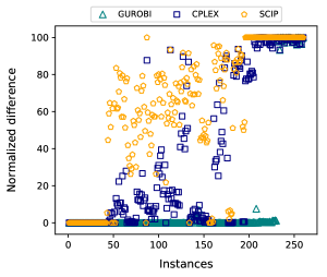
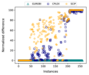
Under 60-second time limit, GUROBI outperforms both CPLEX and SCIP for small and moderate-size instances. As the instances become larger, the upper bounds provided by GUROBI and CPLEX become closer. When we increase the time limit to 10 minutes, the solution quality of GUROBI considerably improves especially for large instances, while CPLEX and SCIP produce almost the same results as before.
Comparison of DA modes. Next, we evaluate the performances of normal and parallel modes of DA. When running the normal mode of DA, we used the best parameter combination we found after some preliminary testing, although we do not claim it to be the best possible of all, and for the parallel mode, we used the default hyperparameters, as mentioned at the beginning of Section 3. Figure 2 shows the performance of DA in terms of normalized differences, with GUROBI’s upper bound values from 60-second and 10-minute experiments being used as reference, provided in Figures 2(a) and 2(b), respectively.
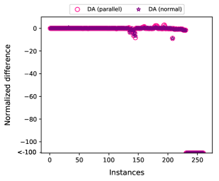
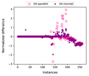
We observe that the two modes of DA yield almost the same level of performance, with the normal mode being slightly better than parallel. Moreover, the average running time of the normal mode (0.40 second) is significantly less than that of parallel mode (67.03 seconds). Since these plots are constructed by taking the upper bound values from GUROBI as a reference, they also implicitly compare the performances of DA and GUROBI under 60-second and 10-minute time limits. We see from Figure 2(a) that for small and moderate-size instances, both modes of DA and GUROBI provide similar upper bounds under 60-second time limit. As the instance size increases, the upper bounds provided by DA become significantly better than those of GUROBI. Though GUROBI is able to yield improved solutions when the time limit is increased to 10 minutes, for large instances it is still outperformed by DA. So, we conclude that DA is particularly effective in tackling large instances where exact solvers start struggling.
Variable ordering analysis. We now analyze the effect of input format on the performance of DA, namely the impact of different variable orderings, inspired by the observation that it can significantly affect the performance of established solvers in solving mixed-integer linear programs (see for instance (Achterberg and Wunderling 2013)). For this purpose, we take a sample of five pure QUBO problem instances with 1000 variables, and experiment with 100 different random permutations of variable indices, using both modes of DA. For normal mode, we test two different parameter combinations; an arbitrarily selected one that is not specifically tuned, and one that is the best we obtained as a result of some preliminary experiments.
Table 2 summarizes the results of our tests with different variable orderings. For each one of the three alternative configurations, namely the parallel mode (“Parallel”), normal mode with an arbitrary parameter configuration (“Normal”), and normal mode with a tuned parameter combination (“Normal (tuned)”), we provide the average of the best found objective values for 100 random permutations of variable indices. In order to examine possible effects of the number of iterations, we conduct this experiment using two different settings for it; and iterations. In the last row of the table, we also report the average percentage difference (“Avg % diff”) of the objective values corresponding to the best and worst orderings, where the differences are normalized with respect to the worst ordering.
| iterations | iterations | |||||
|---|---|---|---|---|---|---|
| Instance | Normal | Normal | Parallel | Normal | Normal | Parallel |
| (tuned) | (tuned) | |||||
| bqp_1000_1 | ||||||
| bqp_1000_2 | ||||||
| bqp_1000_3 | ||||||
| bqp_1000_4 | ||||||
| bqp_1000_5 | ||||||
| Avg % diff |
The results indicate that while the impact of variable ordering is insignificant when the number of iterations is large, it does make a difference when the number of iterations is low, as the average percentage differences reveal. Additionally, we observe that when the parameters for normal mode are not tuned, there is room for improvement through different variable orderings. In particular, with a relatively small number of iterations, the difference between the best and worst variable ordering decreases from about 42% to 25% with the tuning of parameters, which is a significant improvement. So, we conclude that, when the number of iterations is high, DA becomes insensitive to the input format and demonstrates a more robust performance.
Overall performances. Finally, we present a summary of our computational results on pure QUBO instances in Table 3, which contains average normalized differences with 10-minute results of GUROBI taken as reference (“Norm diff”), average percentage gaps with respect to the best lower bound found (“% gap”), average percentage gaps reported by solvers (“% solver gap”), as well as average run times (“Time (sec)”). The signs in the table stand for values that are greater than . The results indicate that DA both in normal and parallel modes outperforms the other solvers both in terms of solution quality and run times.
| 60-sec limit | 120-sec limit | 10-min limit | ||||||||||
|---|---|---|---|---|---|---|---|---|---|---|---|---|
| DA (n) | DA (p) | GUROBI | CPLEX | SCIP | DA (p) | GUROBI | CPLEX | SCIP | GUROBI | CPLEX | SCIP | |
| Norm diff | -0.1 | -0.1 | 11.6 | 36.9 | 60.2 | -0.2 | 9.7 | 34.3 | 58.0 | 0.0 | 32.3 | 55.1 |
| % gap | 9.2 | 9.2 | 9.1 | 9.3 | ||||||||
| % solver gap | – | – | – | 9.9 | ||||||||
| Time (sec) | 0.4 | 67.0 | 48.5 | 48.1 | 50.1 | 112.6 | 96.2 | 96.2 | 98.5 | 472.4 | 487.8 | 480.0 |
3.2 Quadratic assignment problem
In this section, we focus on the well-known quadratic assignment problem, QAP. It is typically formulated as a constrained model, but can easily be reformulated as a QUBO model as well, because the original constraints are equalities and all the decision variables are binary.
QAP is one of the most difficult COPs and has appeared in many practical applications, including economic problems, scheduling, hospital planning, placement of electronic components, and many more. Different mathematical formulations (e.g., integer and mixed-integer linear, permutation-based, graph-based formulations), heuristics (e.g., local search, tabu search, simulated annealing, genetic algorithms) and exact solution approaches (e.g., branch-and-bound, cutting plane algorithms, dynamic programming) have been proposed for it. For more information on QAP, we refer the reader to the survey by Loiola et al. (2007).
In what follows, we consider the IP formulation initially proposed by Koopmans and Beckmann (1957), reformulate it as a QUBO model, and present the results of our experiments using these models with DA and the three solvers.
3.2.1 Formulations
We are given a set of facilities and candidate locations. For each pair of locations , a distance parameter , and for each pair of facilities , a flow parameter is defined. The goal is to assign each facility to a distinct location by minimizing the sum of the product of distances with the corresponding flows. To this end, we define a set of binary decision variables:
Using the parameters and variables as defined above, an IP formulation for QAP can be written as follows:
| (8a) | |||||
| s.t. | (8b) | ||||
| (8c) | |||||
| (8d) | |||||
The quadratic objective function (8a) minimizes the total cost of the assignment. Constraints (8b) ensure that each location is assigned exactly one facility, and (8c) guarantee that each facility is assigned to a single location. Finally, constraints (8d) enforce the decision variables to be binary.
Dualizing the equality (assignment) constraints, we obtain the following QUBO formulation of QAP:
| (9a) | ||||
| s.t. | (9b) | |||
3.2.2 Experimental results
We collected 136 QAP instances from the well-known library named QAPLIB444 http://qplib.zib.de (Furini et al. 2018). The instances have 100 to 10000 variables. After filtering the instances that are size-wise eligible for DA, a total of 123 instances remained. We conducted our computational experiments on those instances, using the three state-of-the-art solvers to solve the associated IP and QUBO formulations, and DA for solving the QUBO formulations. Since it takes less than two minutes for DA to solve each of these instances, we used 60- and 120-second time limits in our experiments to compare the performances of solvers on equal terms. In addition, we conducted 10-minute experiments using GUROBI, CPLEX and SCIP in order to see how much their solution quality improves when a longer time is allowed. We used a penalty coefficient () value of 16,000 in our QUBO experiments, which, among the ones we tested, led to the best overall results for DA. In particular, higher values, combined with the instance coefficients in our test bed, went beyond the acceptable ranges for DA, where smaller values led to lower feasibility percentages.
Feasibility analysis. Our first observation from our experiments is that, when solving the QUBO formulations, the solvers fail to yield feasible solutions for a significant portion of the QAP instances. Therefore, we begin with analyzing how much the solvers succeed in yielding feasible solutions. Table 4 reports the feasibility percentage of the solutions obtained within 120-second time limit (“% feas”), as well as the average percentage gap of the solvers on the instances for which DA fails to find any feasible solutions (“% solver gap”).
| IP | QUBO | |||||||
|---|---|---|---|---|---|---|---|---|
| GUROBI | CPLEX | SCIP | DA (n) | DA (p) | GUROBI | CPLEX | SCIP | |
| % feas | 100.0 | 100.0 | 100.0 | 63.4 | 63.4 | 61.0 | 57.7 | 6.5 |
| % solver gap | 84.7 | 88.5 | 93.8 | – | – | – | – | – |
| (DA infeas) | ||||||||
From the first row of the table, we observe that GUROBI, CPLEX and SCIP are able to find feasible solutions to the IP formulations of all QAP instances within the time limit. However, as QUBO solvers, they fail to find any feasible solutions for a considerably large subset of instances. Among QUBO solvers, both normal and parallel modes of DA outperform the others in providing feasible solutions. Furthermore, the second row of the table indicates that although exact IP solvers can find feasible solutions for all of the instances, their average percentage gaps are too high in the instances for which DA fails to find any feasible solutions. Moreover, GUROBI, CPLEX and SCIP as QUBO solvers cannot find feasible solutions for all of those instances within the time limit. These findings imply that those instances are too hard thus the solvers struggle in finding high-quality solutions.
In order to gain further insight into the feasibility percentage of the solutions DA yields, we chose a subset of instances and scaled down the coefficients of the distance and flow matrices by dividing them by a constant number. We selected this subset in such a way that it contains instances where DA performs well, moderately and poorly, so that the results obtained on this test set can be reliably generalized. We have seen that with the new scaling, the feasibility percentage in DA’s solutions on the selected set of instances increases from about 34% to 75%, implying that the performance of DA is sensitive to the magnitude of the input coefficients.
In the sequel, we present the experimental results obtained on the original QAP instances. Each figure shows the results from a list of common instances eligible for a particular comparison, with the -axes representing instances sorted in ascending order with respect to the number of variables they contain. We begin with comparing the modes of DA, and then solvers GUROBI, CPLEX, and SCIP to each other both as IP solvers and QUBO solvers.
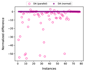
Comparison of DA modes. Figure 3 illustrates the performance of DA in normal and parallel modes on the basis of normalized difference of the upper bound values. Here, the objective values from the normal mode of DA is taken as reference in order to fix one set of data points to zero level and thereby facilitate the comparison. We observe that parallel mode of DA outperforms normal mode especially on small and medium-size instances, because the majority of the data points for the parallel mode of DA lies below the zero level.
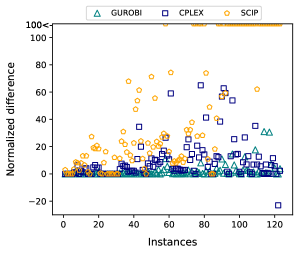
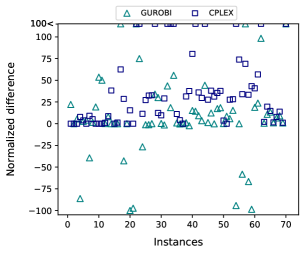
Comparison of exact solvers. Next, we compare GUROBI, CPLEX and SCIP to each other in Figure 4. In this case, we take GUROBI’s 10-minute performance (as IP solver) as reference and report the normalized differences with respect to the objective values thereof. Figure 4(a) shows the results from the three solvers in solving the IP formulations under 120-second time limit. We see that GUROBI performs better than CPLEX and SCIP in almost all the instances, and SCIP performs poorly especially for large instances, as revealed by the data points with a normalized difference value of larger than 100. In comparing the performances in solving the QUBO formulations, we exclude SCIP, because it can barely find any feasible solutions (as reported in Table 4). The results from GUROBI and CPLEX under 120-second time limit provided in Figure 4(b) indicate that GUROBI mostly outperforms CPLEX in solving the QUBO formulations of the QAP instances. Additionally, for a subset of instances, GUROBI as QUBO solver provides better solutions than it does as IP solver.
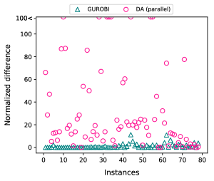
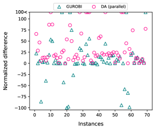
Comparison of DA and exact solvers. Based on the above results, we choose GUROBI and parallel mode of DA for further evaluation, and compare them in Figure 5 using their 120-second performances. From Figures 5(a) and 5(b), we see that GUROBI as IP solver always yields at least as good or better objective values than DA, where DA occasionally does better than GUROBI as QUBO solver. As we take GUROBI’s 10-minute results as reference, Figure 5(a) also implies that GUROBI cannot really improve the quality of the solutions with increased time limit, because the normalized differences are almost always zero.
Overall performances. We conclude our experimental analysis for QAP with an overall summary of the computational results, provided in Table 5. The table reports the average normalized differences with 10 minute results of GUROBI as IP solver taken as reference (“Norm diff”), average run times (“Time (sec)”), and average percentage gap provided by each solver (“% solver gap”), for DA and the other three as IP solvers. All of the reported results are calculated for a set of common instances for which all solvers can provide feasible solutions in the given time limits. As before, the signs in the table stand for values that are greater than . The average performance of GUROBI is better than the other exact solvers and DA in terms of solution quality. In terms of run times, on the other hand, DA in normal mode is able to provide feasible solutions in less than half a second.
| 60-sec limit | 120-sec limit | 10-min limit | |||||||||
|---|---|---|---|---|---|---|---|---|---|---|---|
| DA (n) | GUROBI | CPLEX | SCIP | DA (p) | GUROBI | CPLEX | SCIP | GUROBI | CPLEX | SCIP | |
| Norm diff | 66.7 | 1.9 | 9.9 | 37.5 | 1.0 | 8.0 | 0.0 | 5.2 | |||
| Time (sec) | 0.4 | 46.4 | 49.3 | 57.3 | 106.8 | 90.3 | 95.5 | 112.1 | 417.1 | 460.5 | 509.3 |
| % solver gap | – | 63.7 | 71.3 | 91.1 | – | 59.4 | 69.6 | 86.8 | 53.5 | 63.6 | 76.9 |
3.3 Quadratic cycle partition problem
In this section, we explore a graph application, which, to the best of our knowledge, has not been addressed with DA or similar solution technologies before. Given a graph with vertex set and arc set , a cycle partition is a set of (directed) cycles such that every vertex is contained in exactly one cycle. The cycle partition problem aims to find a cycle partition of minimum (or maximum) weight, and in that regard the well-known travelling salesperson problem is a special case of it. The cycle partition problem can be defined on undirected graphs as well, but in this study, we consider the problem on directed graphs. In particular, we consider the quadratic cycle partition problem (QCPP), which aims to find a cycle partition in a directed graph so that the sum of the interaction costs between consecutive arcs is minimized.
QCPP is an important problem in that it is closely related to the quadratic traveling salesperson problem (Jäger and Molitor 2008), and has many variants with applications in various fields (De Meijer and Sotirov 2020a). Different solution approaches for QCPP or its variants have been studied in the literature, such as local search methods, column generation to compute lower bounds, and branch-and-bound algorithms (Jäger and Molitor 2008; Galbiati, Gualandi, and Maffioli 2014). In the sequel, we test the IP, QUBO, and DA approaches on QCPP.
3.3.1 Formulations
QCPP can be formulated as an IP model containing only binary variables and equality constraints. Suppose that we are given a directed graph with vertex set and arc set , and arc pair costs ’s for all . The cost of an arc pair is nonzero only if the associated arcs are consecutive, that is, if the vertex of arc is directed to and the vertex of arc is directed from are the same. Let and respectively denote the set of all outgoing and incoming arcs of vertex . We define binary decision variables ’s for the assignment of arcs to cycles as such:
Then, an IP formulation for QCPP can be written as follows:
| (10a) | |||||
| s.t. | (10b) | ||||
| (10c) | |||||
| (10d) | |||||
The quadratic objective function (10a) minimizes the total interaction cost between selected arcs. Constraints (10b) and (10c) ensure that each vertex must be incident to exactly one cycle. Constraints (10d) restrict the decision variables to be binary.
Similar to QAP, we can dualize the equality constraints by taking the square of the difference between the left- and right-hand sides of each constraint and adding them to the objective as penalty terms. Then, a QUBO formulation for QCPP can be written as follows:
| (11a) | ||||
| s.t. | (11b) | |||
where is the penalty coefficient. For a sufficiently large value of , the QUBO formulation (11) produces provably optimal solutions for the original IP model (10).
3.3.2 Instances
We generated 80 QCPP instances of varying sizes by following the procedure in (De Meijer and Sotirov 2020b). Specifically, we first created the graph instances according to the Erdős and Rényi (1959) model, where each possible arc is added with a certain probability. For each graph instance, the interaction cost between any pair of successive arcs is chosen as an integer uniformly distributed between 0 and 100. The number of vertices in our instances vary between 25 to 175, and the arc densities range from 0.25 to 0.75. We note that the instances used in (De Meijer and Sotirov 2020b) are relatively small, and typically easy to handle by the state-of-the-art solvers now. Thus, we created our test bed by including larger and hence more challenging QCPP instances. We provide brief information on our test bed in Table 6.
| # instances | # vertices | Density | # variables |
|---|---|---|---|
| 80 | 25–175 | 0.25, 0.50, 0.75 | 127–7963 |
In order to ensure that our model correctly represents the problem for each instance, we made sure that every vertex of a graph instance has at least one incoming and one outgoing arc, because otherwise there will be at least one vertex for which constraints of type (10b) and (10c) are incomplete or absent in the model, which would lead to an incorrect representation of the problem. Even though we ensure that all the required constraints are contained the IP model, it is not trivial to guarantee the existence of a cycle partition in a graph, mainly because every vertex needs to be covered by exactly one cycle. Nonetheless, all the problem instances in our test bed have a nonempty feasible solution space.
3.3.3 Experimental results
In this section, we present the results of our computational study for QCPP, starting with pictorial expositions and concluding with tabular summaries. The points on the -axes of figures represent individual instances arranged in ascending order with respect to the number of variables they have. We use normalized differences as a means to compare solvers, where the objective values (upper bounds) from GUROBI’s 10-minute experiments are taken as reference.
Comparison of exact solvers. We first compare the performances of GUROBI, CPLEX and SCIP in solving the IP formulations in terms of normalized differences, shown in Figure 6.
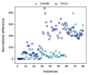
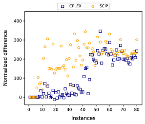
Figure 6(a) contains the normalized differences of 60-second results from GUROBI and CPLEX. In this case, we do not include SCIP, because it failed to deliver any valid lower or upper bounds, even when the time limit is increased to 120 seconds. Our observation is that GUROBI does better than CPLEX especially in small to moderate-size instances. Specifically, GUROBI does at least as good as CPLEX in 72.5% of the instances.
We also compare the performance of solvers under 10-minute time limit, shown in Figure 6(b). Here, we do not explicitly show the results from GUROBI, because the associated upper bound values are taken as reference and hence the corresponding normalized difference values would simply be anchored at zero level. We see from this figure that both CPLEX and SCIP almost always yield inferior upper bounds as compared to GUROBI, because the data points are almost always above zero. While CPLEX and SCIP perform the same on small instances, CPLEX does typically better than SCIP in the rest, and the difference is especially noticable in moderate-size instances. In particular, CPLEX does at least as well as SCIP in 91.3% of the instances. As a result of this comparative evaluation, we continue with GUROBI to compare DA to, as it yields the most promising results among the three solvers.
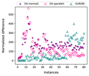
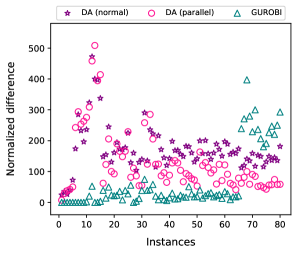
Comparison of DA and exact solvers. Figure 7 shows the normalized differences for GUROBI and both modes of DA. We see that GUROBI yields better objective values than DA for relatively small instances. On the other hand, for larger instances, i.e., when we look at the data points towards the right end of the -axis, both normal and parallel modes of DA yield significantly better objective values, with the parallel mode being the best among all. Particularly, for 60- and 120-second results, DA outperforms in approximately 29% and 19% of the instances with at least 4500 and 7100 variables, respectively. So, the gap between the data points corresponding to GUROBI and the parallel mode of DA is greater for larger instances, and that DA shows a robust performance despite increasing instance sizes. Therefore, we conclude that DA is particularly successful in yielding good-quality solutions quickly for large instances.
Penalty coefficient analysis. Next, we investigate the effect of the penalty coefficient values on DA’s performance. Figure 8 shows the average of the best objective values found by DA using six different penalty coefficient values. The lower end of the values are determined in such a way that DA is able to yield a feasible solution to the entire set of instances we experiment with, and the largest value is set so that the general trend in the performances can be observed.
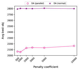
We first see that the parallel mode of DA delivers significantly better results than the normal mode on the average. In addition, setting gives the least overall average values for parallel mode, and the performance keeps deteriorating for larger values of the penalty coefficient . As the parallel mode yields better results in general, we took its minimum point as a reference and used when running the QUBO models for QCPP, i.e., in obtaining the above-presented results. We note that even if we were to carry out our comparative analysis with a different penalty coefficient, our conclusions would not generally change, because the difference it would create in DA’s performance is less than how much it differs from GUROBI for cases where DA outperforms.
Overall performances. In the remainder of this section, we provide tabular summaries of overall performances. We start with the average performance of solving the QUBO formulations with DA in comparison to solving the IP formulations with GUROBI, CPLEX and SCIP under different time limits, reported in Table 7. The table contains three blocks of columns reserved for different time limits, and another column dedicated to the normal mode of DA only, because its execution times do not exceed half a second even when the number of iterations is increased greatly. The blocks contain the results of solving the QUBO formulations with DA and/or solving the IP formulations with GUROBI, CPLEX and SCIP. For each option (column), we report the averages of best found objective values (“UB”), normalized differences with 10 minute results of GUROBI as IP solver taken as reference (“Norm diff”), and solution times (“Time (sec)”). We note that the normalized differences are calculated by taking the objective values from 10-minute experiments with GUROBI as reference, because it yielded the best values. Furthermore, SCIP is excluded from 60-second and 120-second blocks, because it failed to yield any valid lower or upper bound within these time limits.
| 60-sec limit | 120-sec limit | 10-min limit | ||||||||
|---|---|---|---|---|---|---|---|---|---|---|
| DA (n) | DA (p) | GUROBI | CPLEX | DA (p) | GUROBI | CPLEX | GUROBI | CPLEX | SCIP | |
| UB | 2803.7 | 2059.5 | 2573.5 | 3311.9 | 2057.6 | 2152.6 | 3222.1 | 1105.7 | 2812.9 | 3522.4 |
| Norm diff | 172.1 | 129.5 | 90.0 | 173.3 | 128.2 | 63.8 | 161.6 | 0.0 | 112.6 | 199.3 |
| Time (sec) | 0.4 | 61.7 | 56.3 | 57.4 | 103.8 | 112.0 | 114.4 | 541.0 | 563.7 | 567.1 |
| % gap | 91.8 | 91.8 | 84.0 | 86.7 | 91.7 | 83.3 | 85.8 | 82.2 | 83.5 | 88.0 |
| % solver gap | – | – | 87.1 | 93.0 | – | 85.0 | 92.5 | 82.2 | 90.5 | 93.5 |
Under 60-second and 120-second time limits, parallel mode of DA gives the best average upper bounds, and the difference from other solvers is considerably large in the 60-second case. As for the normal mode, its average upper bound value is better than those obtained from CPLEX and SCIP under 10-minute limit, and its execution time is only 0.4 second. In terms of the average normalized differences, GUROBI averages are the best under all three time limits. Combining these aggregated results with those over the individual instances discussed above, we can say that DA is particularly successful in yielding good-quality solutions for relatively large instances, and if such solutions are needed within a second, normal mode of DA is the most promising option. We note that all the solutions that DA yield are feasible, and hence is not explicitly reported in the table.
We finally evaluate the overall performances of GUROBI, CPLEX and SCIP in solving the QUBO formulations, and report the associated results in Table 8. In this case, since we are solving QUBO models, we include the feasibility percentage of found solutions (“% feas”) in addition to the three measures used in Table 7. We show values that are greater than with the sign in the table.
| 60-sec limit | 120-sec limit | |||||
| GUROBI | CPLEX | SCIP | GUROBI | CPLEX | SCIP | |
| UB | 91802.8 | 6143.7 | 158424.1 | 77820.2 | 5967.7 | 157672.9 |
| Norm diff | 5701.4 | 453.3 | 4106.9 | 416.5 | ||
| Time (sec) | 60.8 | 103.3 | 60.4 | 120.2 | 138.6 | 121.1 |
| % feas | 55.0 | 30.0 | 0.0 | 67.5 | 32.5 | 6.3 |
| % gap | 86.5 | 89.3 | 99.5 | 86.2 | 87.5 | 96.4 |
| % solver gap | 2507.5 | 2068.5 | ||||
We see that SCIP fails to deliver any feasible solution within one minute, and in two minutes, it achieves feasibility in only 6.3% of the instances. Even though GUROBI and CPLEX do significantly better relative to SCIP, their performance as QUBO solvers is still not satisfactory; the feasibility percentage goes only as much as 67.5% in the best case. So, we conclude that DA is the best QUBO solver, and yields the best results for large-scale instances in cases where short solution times are sought.
3.4 Selective graph coloring problem
In this section, we focus on the selective graph coloring problem, Sel-Col, which is a generalization of the classical graph coloring problem. Coloring of a graph is assignment of labels (colors) to its vertices, such that no pair of vertices that are linked by an edge receives the same color. Given a graph and a partition of its vertex set into clusters, the aim in Sel-Col is to choose exactly one vertex per cluster so that, among all possible selections, the number of colors necessary to color the selected set of vertices is minimized. As opposed to the classical graph coloring problem, we do not color every vertex in this problem; we only do so for the selected set. Figure 9 illustrates a small Sel-Col instance together with one feasible and one optimal selective coloring of it. To the best of our knowledge, this problem has not been addressed with DA or similar solution technologies before.
Sel-Col has emerged as a model to select a route and assign a proper wavelength to each in the second step of a two-phase solution strategy for the routing and wavelength assignment problem that arises in optical networks (Li and Simha 2000). The problem has many applications in various domains, such as timetabling, constraint encoding, antenna positioning and frequency assignment (Demange et al. 2015). Several solution approaches have been proposed for Sel-Col, for general instances or specific graph classes, including heuristics (Li and Simha 2000), and exact algorithms such as a branch-and-cut algorithm (Frota et al. 2010), branch-and-price algorithms (Hoshino, Frota, and De Souza 2011; Furini, Malaguti, and Santini 2018), and cutting plane algorithms (Şeker, Ekim, and Taşkın 2019, 2020). In what follows, we present the results of IP, QUBO and DA approaches in handling Sel-Col.
3.4.1 Formulations
Suppose that we are given an undirected graph with , as well as a partition of its vertex set into clusters . Sel-Col can be formulated as an IP model, which only contains binary variables but has both equality and inequality constraints. We introduce two sets of binary variables. First, we define ’s for to keep track of the number of colors used.
Second, we define ’s for in order to relate the color usage to the assignment of colors to vertices.
Then, an IP formulation for Sel-Col, which appears in (Şeker, Ekim, and Taşkın 2019, 2020), can be written as follows:
| (12a) | |||||
| s.t. | (12b) | ||||
| (12c) | |||||
| (12d) | |||||
| (12e) | |||||
| (12f) | |||||
The objective function (12a) minimizes the number of colors used. Constraints (12b) guarantee that exactly one vertex is selected per cluster. The requirement that adjacent vertices cannot be assigned the same color is met through constraints (12c). Constraints (12d) link and variables by forcing to be one if color is used by some vertex. Finally, (12e) and (12f) respectively set and to be binary variables. Note that as we are minimizing the number of colors used, when for some , then in any optimal solution.
Despite the presence of inequality constraints, we can reformulate the IP model in (12) as a QUBO formulation without any need to introduce additional variables. We note that the inequality constraints (12c) and (12d) can be equivalently written as a pair of quadratic equality constraint sets as such:
| (12c - q) | ||||
| (12d - q) | ||||
The set of feasible and values induced by (12c) and (12d) are the same as those enforced by (12c - q) and (12d - q). Therefore, we can safely replace the inequalities with the equivalent quadratic set of inequalities, and transform the IP model into the following QUBO model:
| (13a) | ||||
| s.t. | (13b) | |||
| (13c) | ||||
3.4.2 Size reduction
For our computational experiments, we consider a large suite of 1200 Sel-Col instances. One half of the instances contain perfect graphs, and the other half Erdős and Rényi (1959) graphs. We refer to these two groups as PG and ER instances, respectively. When we first transformed the IP formulations of these Sel-Col instances into QUBO models, around 37% of them were size-wise eligible for DA. This inclined us to explore ways to reduce the sizes of these instances in order to make a larger proportion fit into DA. For this purpose, we design a two-phase heuristic to decrease the number of variables.
Our heuristic is inspired from the fact that Sel-Col naturally consists of two parts; the vertex selection, and the coloring of it. In the first phase of our heuristic, we choose one vertex per cluster that has the least number of connections to other clusters. By doing so, we aim to decrease the number of edges between the selected set of vertices, and hence potentially the number of colors required (although decreasing the number edges in a graph does not necessarily reduce the number of colors needed). In the second phase, we use a heuristic coloring algorithm to color the selected set of vertices, where in each step we color a vertex that has the largest number of already colored neighbors, similar to the DSatur algorithm (Brélaz 1979). This yields an upper bound on the minimum number of colors needed to color the given vertex selection from the first phase, which also serves as an upper bound on the optimal number of colors of that Sel-Col instance. This way, we eliminate the need of defining decision variables with a color index larger than the upper bound found. This technique can be viewed as a variant of the size reduction ideas proposed by Lewis and Glover (2017), where variables are identified and eliminated based on optimality conditions by examining the matrix of objective coefficients.
After applying the size reduction procedure, out of 1200 Sel-Col instances (to be described in the next section), 1131 became size-wise suitable for DA. Table 9 gives the percentage of instances that fit into DA before and after the size reduction operation, as well as the percentage reduction in the number of variables, separately for PG and ER instances. We see that our heuristic procedure increases the number of instances eligible for DA by more than 60% and 53% for the two instance groups, by reducing their sizes around 85% on the average.
| % eligible for DA | % | ||
|---|---|---|---|
| Before | After | reduction | |
| PG | 37.0 | 97.5 | 88.8 |
| ER | 37.2 | 91.0 | 80.6 |
3.4.3 Instances
A Sel-Col instance is comprised of a graph and a partition of its vertex set, i.e., a set of clusters. Our instances are based on 400 distinct graph instances, with 200 being perfect graphs, and 200 Erdős and Rényi (1959) type graphs. The graphs contain 50 to 500 vertices and have average edge densities ranging from 0.1 to 0.7. The full set of Sel-Col instances are obtained by combining each graph with three different sets of clusters, where the number of vertices in each cluster vary between 2–5, 4–7, and 6–9. So, from each of the 400 graph instances, three different Sel-Col instances are generated, which makes a total of 1200 instances, where the ones based on perfect graphs are those used in (Şeker, Ekim, and Taşkın 2020). Brief descriptive information about our test bed, which we obtained after applying the two-phase heuristic procedure explained above, is provided in Table 10. The two rows of the table are reserved for the two groups of instances, PG and ER, and the columns respectively provide the number of instances, the range of the number of vertices, the edge densities of graphs, the range of the number of clusters, the range of the number of available colors in the IP and QUBO models (“# avail colors”), and the range of the number of variables in these instances.
| # instances | # vertices | Density | # clusters | # avail colors | # variables | |
|---|---|---|---|---|---|---|
| PG | 586 | 50–500 | 0.1, 0.3, 0.5, 0.7 | 6–150 | 1–22 | 51–7722 |
| ER | 547 | 50–500 | 0.1, 0.3, 0.5, 0.7 | 6–152 | 1–25 | 51–8118 |
3.4.4 Experimental results
We now present the results of our computational study that we conducted on our Sel-Col test bed. As before, we employed DA, GUROBI, CPLEX and SCIP in our experiments, and used 30- and 60-second time limits. We additionally tested GUROBI and CPLEX under a 10-minute limit to observe how much more they could achieve if longer solution times were allowed. When solving the IP models with GUROBI and CPLEX, we have incorporated a set of symmetry breaking constraints, which are used in (Şeker, Ekim, and Taşkın 2019, 2020), in order to reduce the number of different representations of equivalent solutions in the feasible solution space. In addition, we fed the solution found through our two-phase heuristic as a warm-start to the IP solvers. In the figures that follow, we present the results of our experiments under 30-second time limit, but we note that the general picture does not change much in the 60-second experiments. The points on the -axes of figures represent individual instances sorted in ascending order with respect to the number of variables they contain.
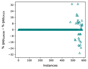
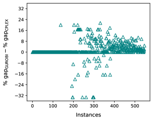
Comparison of exact solvers. We start with comparing the performances of GUROBI and CPLEX on the basis of the upper bounds they provide, i.e., the objective values of the best feasible solutions found. We note that this measure is interesting for this problem class since the optimal values (i.e., the minimum number of colors needed) are usually small, and it thus provides a better idea on the quality of the obtained solutions than the optimality gaps. Figure 10 presents the difference between the upper bounds from the two solvers. The number of instances being high, we plot the differences rather than the individual upper bounds in order to make the exposition of the comparison easily interpretable. Since we subtract the upper bound values from CPLEX from those of GUROBI, a data point above the zero level means that GUROBI is outperformed by CPLEX for the associated instance. Conversely, a data point lying below the zero level indicates that GUROBI outperforms for that instance.
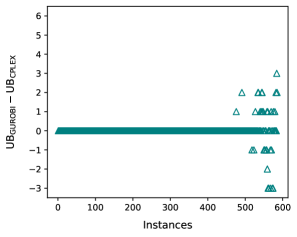
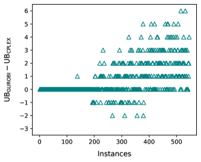
For PG instances, GUROBI and CPLEX yield the same objective values in about 94% of the instances (zero level), and there is no obvious outperformance of either in the rest. For ER instances, on the other hand, CPLEX shows a better performance than GUROBI by yielding smaller and same objective values in nearly 37% and 58% of the instances, respectively.
The upper bound differences provide a comparison in terms of the quality of the feasible solutions provided, but do not say much on how close the solutions are to the optimals, because the lower bounds are absent in the analysis. Therefore, we next compare the performances using the difference in percentage optimality gaps with respect to the best lower bound values available (“% gap”) in Figure 11. As before, we plot the differences, rather than the individual percentage gap values separately for each solver, in order to avoid a convoluted picture arising from overlapping data points. Our observation is that the percentage gap values of GUROBI and CPLEX are the same in the majority of instances (zero level), and in most of the remaining, CPLEX yields better results (above the zero level). This indicates that CPLEX usually yields better solutions than GUROBI, and the difference is more evident in ER instances. Hence, we continue our evaluation using the results of CPLEX.
Comparison of DA and CPLEX. We now compare DA’s performance to CPLEX. Figure 12 presents the difference of the DA’s objective values in normal and parallel modes from those of the CPLEX.
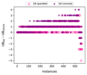
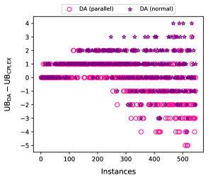
For the majority of PG instances, the quality of the objective values found by DA are at most two units worse than those of CPLEX, but the overall performance of CPLEX is better than both modes of DA. In particular, normal and parallel modes of DA yield at least as good results in nearly 21% and 39% of the PG instances. For ER instances, however, normal mode of DA performs at least as well as CPLEX in 39% of the instances, while it becomes more than 61% for the parallel mode. So, parallel mode of DA is successful in yielding good-quality solutions especially for ER instances.
Having evaluated the performance of DA in comparison to CPLEX, we now investigate the marginal contribution of DA on top of the objective values achieved by our two-phase heuristic. Figure 13 shows the difference of DA’s objective values from those of the two-phase heuristic.
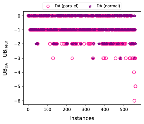
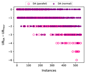
We observe that the amount of improvement, if any, ranges from one to six units, and the parallel mode of DA performs somewhat better than the normal mode. Specifically, DA improves upon the two-phase heuristic in nearly 50% and 78% of PG instances with normal and parallel modes, respectively, while these percentages increase to 62% and 88% for ER instances. So, especially the parallel mode of DA improves the solution quality in the majority of instances, if there is any room for it, and the improvement manifests more evidently in ER instances.
Penalty coefficient analysis. Next, we investigate the effect of the penalty coefficient values on DA’s performance. For Sel-Col, the maximum value that the objective function can take is the number of available colors. Moreover, if a solution to the QUBO model in (13) violates some of the original constraints in (12b)–(12d), the magnitude of violation is at least one. Then, a penalty coefficient () value strictly larger than the number of available colors leads to a penalty greater than the largest possible objective value any feasible QUBO solution can yield, and hence the value of the QUBO objective for an optimal solution always lies below those that are infeasible for the IP model, rendering the QUBO formulation in (13) exact. Let denote the number of available colors (which can at most be equal to the number of clusters ). Though is sufficient to make the QUBO model exact, we experimented with various penalty coefficient values as a function of the number of available colors to test the effect on the performance of DA. Figure 14 shows the average objective values from both modes of DA for different penalty coefficient settings.
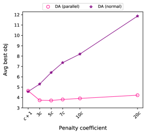
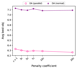
We see from Figures 14(a) and 14(b) that the effect of the penalty coefficient value manifests differently in normal and parallel modes, and in PG and ER instances. Even though smaller penalty coefficient values typically lead to improved performance in DA, as analyzed and reported in (Şeker, Bodur, and Pouya 2020) and mentioned in (Cohen, Senderovich, and Beck 2020; Cohen et al. 2020), it appears from our results in Sel-Col context that higher penalty coefficient values may ameliorate or deteriorate performance, and no strong relationship can be inferred. In our experiments, we used , which we observed to be the best overall option to get the best out of DA. We note that even if we did not make this sensitivity analysis for DA and simply presented the results with , our overall conclusions would not change much, because the marginal improvement it creates for DA does not dominate the performance gap between DA and other solvers.
Overall performances. We conclude this section with tabular summaries of the overall results. Table 11 reports the averages of different performance measures over the PG and ER instances under different time limits. There are two sets of rows, reserved for the results associated with PG and ER instances. For each group of instances, the average of upper bounds (“UB”), percentage of solutions that are feasible (“% feas”), average solution time (“Time (sec)”), average percentage gap with respect to the best lower bound available (“% gap”), and average percentage gap of the solver (“% solver gap”), i.e., gap values using the lower bound values from that solver (rather than the best values) are given. There are four groups of columns, one dedicated for the normal mode of DA, and the other three reserved for the results obtained under the 30-second, 60-second and 10-minute time limits. These column groups contain the results from solving the QUBO formulation with DA and/or solving the IP formulations with GUROBI, CPLEX and SCIP. The reason for the normal mode of DA to comprise a separate group is that no matter how high the number iterations are set, it takes less than a second to solve an instance.
| 30-sec limit | 60-sec limit | 10-min limit | ||||||||
|---|---|---|---|---|---|---|---|---|---|---|
| DA (n) | DA (p) | GUROBI | CPLEX | DA (p) | GUROBI | CPLEX | GUROBI | CPLEX | ||
| PG | UB | 6.4 | 3.7 | 2.9 | 2.9 | 3.7 | 2.9 | 2.9 | 2.7 | 2.7 |
| % feas | 96.7 | 99.5 | 100.0 | 100.0 | 99.5 | 100.0 | 100.0 | 100.0 | 100.0 | |
| Time (sec) | 0.4 | 31.9 | 5.9 | 5.5 | 63.1 | 8.7 | 8.3 | 38.1 | 38.9 | |
| % gap | 25.6 | 25.7 | 1.9 | 1.9 | 25.6 | 1.3 | 1.4 | 0.4 | 0.4 | |
| % solver gap | – | – | 5.6 | 4.6 | – | 3.7 | 3.2 | 0.7 | 0.6 | |
| ER | UB | 7.1 | 6.3 | 7.1 | 6.4 | 6.3 | 6.9 | 6.3 | 6.0 | 6.0 |
| % feas | 100.0 | 100.0 | 100.0 | 100.0 | 100.0 | 100.0 | 100.0 | 100.0 | 100.0 | |
| Time (sec) | 0.4 | 31.3 | 20.2 | 21.5 | 62.2 | 38.5 | 41.3 | 343.9 | 357.2 | |
| % gap | 46.8 | 46.8 | 40.2 | 38.8 | 46.8 | 38.8 | 37.7 | 35.2 | 35.3 | |
| % solver gap | – | – | 49.2 | 47.6 | – | 45.8 | 45.2 | 36.4 | 36.2 | |
Our observation from Table 11 is that under both 30-second and 60-second time limits, the parallel mode of DA yields the best upper bounds for ER instances, and CPLEX is only slightly worse in that regard. Moreover, the upper bounds from 10-minute experiments with CPLEX and GUROBI are not much smaller than those of DA, especially for ER instances. In terms of solution times, GUROBI and CPLEX yield better results than the parallel mode of DA run with default hyperparameters (“DA (p)”). However, the normal mode of DA (“DA (n)”) is extremely fast, and is able to yield good-quality results in less than half a second. For ER instances in particular, we see that the upper bounds from the normal mode of DA are only about one unit away from the 10-minute values of GUROBI and CPLEX. Noting that DA always yields feasible solutions except for a few PG instances, which we see from the “% feas” rows, we can say that the normal mode of DA is by far the best option to obtain good-quality solutions in a very short amount of time, such that GUROBI and CPLEX typically fail to complete even presolve phase of the solution process within that time frame. As for the parallel mode of DA, we see that it is competitive with GUROBI or CPLEX especially in ER instances, which is where they struggle more.
Lastly, we present the results of our experiments where we utilized the three exact solvers to solve the QUBO models for Sel-Col. Table 12 contains the average upper bound, percentage feasibility of solutions, solution time, and percentage gap values from solvers and with respect to the best available lower bound values for GUROBI, CPLEX, and SCIP under 30-second and 60-second time limits. The general structure of this table is the same as that of Table 11. The signs stand for values greater than .
| 30-sec limit | 60-sec limit | ||||||
| GUROBI | CPLEX | SCIP | GUROBI | CPLEX | SCIP | ||
| PG | UB | 450.0 | 280.0 | 1444.8 | 239.7 | 72.3 | 1378.9 |
| % feas | 78.6 | 64.8 | 12.5 | 84.1 | 72.0 | 15.7 | |
| Time (sec) | 27.9 | 28.2 | 29.8 | 54.9 | 55.2 | 59.2 | |
| % gap | 47.4 | 42.8 | 89.5 | 42.6 | 29.7 | 86.9 | |
| % solver gap | |||||||
| ER | UB | 1710.1 | 695.0 | 2395.3 | 1507.9 | 69.0 | 2365.5 |
| % feas | 67.2 | 70.9 | 11.2 | 73.3 | 79.5 | 14.1 | |
| Time (sec) | 28.3 | 32.2 | 30.4 | 55.4 | 64.8 | 59.6 | |
| % gap | 57.9 | 57.6 | 90.3 | 56.2 | 53.3 | 87.8 | |
| % solver gap | |||||||
We see from the “% feas” rows of the table that the feasibility percentages vary between 11% and 85%. Even though the feasibility percentages are not satisfactory in general, the ones from SCIP are far from being at an acceptable level. Since infeasibilities are penalized in the objective function and the penalty coefficient values we use for Sel-Col ensure that the objective values of infeasible solutions are always larger than those of feasible solutions, the average upper bound values are much larger than what they are expected to be even in the worst case. Indeed, the poor performance GUROBI and CPLEX as QUBO solvers is expected, because these solvers are specialized in solving linear and integer linear programs particularly, which is confirmed by their performance in solving the IP formulations, presented above. Overall, we can say that as QUBO solvers, GUROBI and CPLEX are the best among the three alternatives, and the performance SCIP of lies far below the others, which is particularly evident from the percentage of feasible solutions. We note here that even though some of these solvers occasionally yielded invalid lower bounds for quadratic models, which we have observed for some problem classes as mentioned before, we did not obtain any inconsistent results in our Sel-Col experiments. Though this does not prove the validity of the percentage gap values, we nevertheless report them to make our summary table complete and give a general idea on the performances with respect to those measures.
4 Conclusion
In this work, we conduct an extensive computational study to evaluate the performance of the state-of-the-art solvers and DA on various COPs, namely, pure QUBO, quadratic assignment, quadratic cycle partition, and selective graph coloring problems, with the last two being new graph applications for DA. For Sel-Col, we present a two-phase heuristic to reduce instance sizes and thereby improve the extent of instances that DA can handle.
Our results indicate that DA is a viable solution technology for solving problems formulated as QUBO models, usually performs comparable to or better than the state-of-the-art solvers for constrained problems, and is particularly successful in quickly yielding good-quality solutions for large instances where established solvers fail to be useful in limited times.
The number of variables that the current release of DA can handle is 8192, yet it has been recently announced that a new DA technology is developed to help handle up to one million variables (Fujitsu Limited 2020). Considering that DA demonstrates a notably robust performance despite increasing instance sizes without increased execution times, it has the potential to be a viable approach to produce high-quality solutions in a short amount of time for large-scale challenging COPs, for which even the state-of-the-art solution technologies typically struggle.
As a future research direction, the QUBO approach can be coupled with DA technology as part of different algorithms, which is a general strategy used in some existing studies, for instance (Liu et al. 2019; Shaydulin et al. 2019, 2019; Ushijima-Mwesigwa et al. 2020). Such approaches may help overcome the variable size limitation of DA and similar technologies, and also improve the overall solution performance.
Acknowledegments
The authors would like to thank Fujitsu Laboratories Ltd. and Fujitsu Consulting (Canada) Inc. for providing financial support and access to Digital Annealer at University of Toronto. The authors would also like to thank Hamed Pouya for useful discussions at early stages of this work.
References
- Achterberg (2009) Achterberg, Tobias. 2009. “SCIP: solving constraint integer programs.” Math. Program. Comput. 1 (1): 1–41. https://doi.org/10.1007/s12532-008-0001-1.
- Achterberg and Towle (1998) Achterberg, Tobias, and Eli Towle. 1998. “Non-Convex Quadratic Optimization in Gurobi 9.0.” https://pages.gurobi.com/rs/181-ZYS-005/images/2020-01-14_Non%20Convex%20Quadratic%20Optimization%20in%20Gurobi%209.0%20Webinar.pdf.
- Achterberg and Wunderling (2013) Achterberg, Tobias, and Roland Wunderling. 2013. “Mixed integer programming: Analyzing 12 years of progress.” In Facets of combinatorial optimization, 449–481. Springer.
- Aramon et al. (2019) Aramon, Maliheh, Gili Rosenberg, Elisabetta Valiante, Toshiyuki Miyazawa, Hirotaka Tamura, and Helmut G Katzgraber. 2019. “Physics-inspired Optimization for Quadratic Unconstrained Problems Using a Digital Annealer.” Front. Phys. 7: 48.
- Bandyopadhyay et al. (2008) Bandyopadhyay, Sanghamitra, Sriparna Saha, Ujjwal Maulik, and Kalyanmoy Deb. 2008. “A simulated annealing-based multiobjective optimization algorithm: AMOSA.” IEEE Trans. Evol. Comput. 12 (3): 269–283.
- Beasley (1990) Beasley, John E. 1990. “OR-Library: distributing test problems by electronic mail.” J. Oper. Res. Soc. 41 (11): 1069–1072.
- Beasley (1998) Beasley, John E. 1998. “Heuristic algorithms for the unconstrained binary quadratic programming problem.” Technical report, Management School, Imperial College, London, UK.
- Bertsekas (1993) Bertsekas, Dimitri P. 1993. “A simple and fast label correcting algorithm for shortest paths.” Networks 23 (8): 703–709.
- Billionnet and Sutter (1994) Billionnet, Alain, and Alain Sutter. 1994. “Minimization of a quadratic pseudo-Boolean function.” European Journal of Operational Research 78 (1): 106–115.
- Boros, Hammer, and Tavares (2007) Boros, Endre, Peter L Hammer, and Gabriel Tavares. 2007. “Local search heuristics for quadratic unconstrained binary optimization (QUBO).” Journal of Heuristics 13 (2): 99–132.
- Brélaz (1979) Brélaz, Daniel. 1979. “New methods to color the vertices of a graph.” Commun. ACM 22 (4): 251–256.
- Cohen et al. (2020) Cohen, Eldan, Avradip Mandal, Hayato Ushijima-Mwesigwa, and Arnab Roy. 2020. “Ising-Based Consensus Clustering on Specialized Hardware.” In International Symposium on Intelligent Data Analysis, 106–118. Springer.
- Cohen, Senderovich, and Beck (2020) Cohen, Eldan, Arik Senderovich, and J. Christopher Beck. 2020. “An Ising Framework for Constrained Clustering on Special Purpose Hardware.” In International Conference on the Integration of Constraint Programming, Artificial Intelligence, and Operations Research, Springer.
- CPLEX (2009) CPLEX, IBM ILOG. 2009. “V12. 1: user’s manual for CPLEX.” IBM Corp. 46 (53): 157.
- De Meijer and Sotirov (2020a) De Meijer, Frank, and Renata Sotirov. 2020a. “The quadratic cycle cover problem: special cases and efficient bounds.” Journal of Combinatorial Optimization 1–33.
- De Meijer and Sotirov (2020b) De Meijer, Frank, and Renata Sotirov. 2020b. “SDP-based bounds for the Quadratic Cycle Cover Problem via cutting plane augmented Lagrangian methods and reinforcement learning.” arXiv preprint arXiv:2009.03616 .
- Delling et al. (2009) Delling, Daniel, Peter Sanders, Dominik Schultes, and Dorothea Wagner. 2009. “Engineering route planning algorithms.” In Algorithmics of large and complex networks, 117–139. Springer.
- Demange et al. (2015) Demange, Marc, Tınaz Ekim, Bernard Ries, and Cerasela Tanasescu. 2015. “On some applications of the selective graph coloring problem.” European Journal of Operational Research 240 (2): 307 – 314.
- Dijkstra (1959) Dijkstra, Edsger W. 1959. “A note on two problems in connexion with graphs.” Numerische Mathematik 1 (1): 269–271.
- Elsokkary et al. (2017) Elsokkary, Nada, Faisal S Khan, Davide La Torre, Travis S Humble, and Joel Gottlieb. 2017. Financial portfolio management using D-Wave quantum optimizer: the case of Abu Dhabi securities exchange. Technical Report. Oak Ridge National Lab.(ORNL), Oak Ridge, TN (United States).
- Erdős and Rényi (1959) Erdős, Paul, and Alfréd Rényi. 1959. “On Random Graphs.” Publicationes Mathematicae Debrecen 6: 290–297.
- Frota et al. (2010) Frota, Yuri, Nelson Maculan, Thiago F Noronha, and Celso C Ribeiro. 2010. “A branch-and-cut algorithm for partition coloring.” Networks 55 (3): 194–204.
- Fujitsu Limited (2018) Fujitsu Limited. 2018. “Fujitsu Launches Next Generation Quantum-Inspired Digital Annealer Service.” https://www.fujitsu.com/global/about/resources/news/press-releases/2018/1221-01.html.
- Fujitsu Limited (2020) Fujitsu Limited. 2020. “Fujitsu Develops New Tech for Quantum-Inspired “Digital Annealer”, Achieving Megabit-class Performance for Large-Scale Combinatorial Optimization Problems.” https://www.fujitsu.com/global/about/resources/news/press-releases/2020/1109-01.html.
- Furini, Malaguti, and Santini (2018) Furini, Fabio, Enrico Malaguti, and Alberto Santini. 2018. “An Exact Algorithm for the Partition Coloring Problem.” Computers & Operations Research 92: 170–181.
- Furini and Traversi (2013) Furini, Fabio, and Emiliano Traversi. 2013. “Extended linear formulation for binary quadratic problems.” Optimization Online .
- Furini et al. (2018) Furini, Fabio, Emiliano Traversi, Pietro Belotti, Antonio Frangioni, Ambros Gleixner, Nick Gould, Leo Liberti, et al. 2018. “QPLIB: a library of quadratic programming instances.” Math. Program. Comput. 11 (2): 237–265. https://doi.org/10.1007/s12532-018-0147-4.
- Galbiati, Gualandi, and Maffioli (2014) Galbiati, Giulia, Stefano Gualandi, and Francesco Maffioli. 2014. “On minimum reload cost cycle cover.” Discrete Applied Mathematics 164: 112–120.
- Gillett and Miller (1974) Gillett, Billy E, and Leland R Miller. 1974. “A heuristic algorithm for the vehicle-dispatch problem.” Oper. Res. 22 (2): 340–349.
- Giovanni (2017) Giovanni, Luigi De. 2017. “Heuristics for combinatorial optimization.” Course pack for METMODOC: Methods and Models for Combinatorial Optimization, University of Padua. https://www.math.unipd.it/~luigi/courses/metmodoc1819/m02.meta.en.partial01.pdf Accessed 4 August 2020.
- Glover et al. (1999) Glover, Fred, Gary Kochenberger, Bahram Alidaee, and Mohammed Amini. 1999. “Tabu search with critical event memory: an enhanced application for binary quadratic programs.” In Meta-Heuristics, 93–109. Springer.
- Glover, Kochenberger, and Du (2018) Glover, Fred, Gary Kochenberger, and Yu Du. 2018. “A tutorial on formulating and using QUBO models.” arXiv preprint arXiv:1811.11538.
- Glover, Kochenberger, and Alidaee (1998) Glover, Fred, Gary A Kochenberger, and Bahram Alidaee. 1998. “Adaptive memory tabu search for binary quadratic programs.” Management Science 44 (3): 336–345.
- Glover, Lü, and Hao (2010) Glover, Fred, Zhipeng Lü, and Jin-Kao Hao. 2010. “Diversification-driven tabu search for unconstrained binary quadratic problems.” 4OR 8 (3): 239–253.
- Gueye and Michelon (2009) Gueye, Serigne, and Philippe Michelon. 2009. “A linearization framework for unconstrained quadratic (0-1) problems.” Discrete Applied Mathematics 157 (6): 1255–1266.
- Gupta (1971) Gupta, Jatinder N D. 1971. “A functional heuristic algorithm for the flowshop scheduling problem.” J. Oper. Res. Soc. 22 (1): 39–47.
- Gurobi Optimization (2018) Gurobi Optimization, Incorporate. 2018. “Gurobi optimizer reference manual.” https://www.gurobi.com.
- Hasan, Alkhamis, and Ali (2000) Hasan, Merza, Talal Alkhamis, and Jafar Ali. 2000. “A comparison between simulated annealing, genetic algorithm and tabu search methods for the unconstrained quadratic Pseudo-Boolean function.” Computers & industrial engineering 38 (3): 323–340.
- Helmberg and Rendl (1998) Helmberg, Christoph, and Franz Rendl. 1998. “Solving quadratic (0, 1)-problems by semidefinite programs and cutting planes.” Mathematical programming 82 (3): 291–315.
- Hoshino, Frota, and De Souza (2011) Hoshino, Edna A, Yuri A Frota, and Cid C De Souza. 2011. “A branch-and-price approach for the partition coloring problem.” Operations Research Letters 39 (2): 132–137.
- Huang, Pardalos, and Prokopyev (2006) Huang, Hong-Xuan, Panos M Pardalos, and Oleg A Prokopyev. 2006. “Lower bound improvement and forcing rule for quadratic binary programming.” Computational Optimization and Applications 33 (2-3): 187–208.
- Irie et al. (2019) Irie, Hirotaka, Goragot Wongpaisarnsin, Masayoshi Terabe, Akira Miki, and Shinichirou Taguchi. 2019. “Quantum annealing of vehicle routing problem with time, state and capacity.” In International Workshop on Quantum Technology and Optimization Problems, 145–156. Springer.
- Jäger and Molitor (2008) Jäger, Gerold, and Paul Molitor. 2008. “Algorithms and Experimental Study for the Traveling Salesman Problem of Second Order.” In Combinatorial Optimization and Applications, edited by Boting Yang, Ding-Zhu Du, and Cao An Wang, Berlin, Heidelberg, 211–224. Springer Berlin Heidelberg.
- Javad-Kalbasi et al. (2019) Javad-Kalbasi, Mohammad, Keivan Dabiri, Shahrokh Valaee, and Ali Sheikholeslami. 2019. “Digitally Annealed Solution for the Vertex Cover Problem with Application in Cyber Security.” In ICASSP 2019-2019 IEEE International Conference on Acoustics, Speech and Signal Processing (ICASSP), 2642–2646. IEEE.
- Kaveh (2014) Kaveh, Ali. 2014. Advances in metaheuristic algorithms for optimal design of structures. Springer.
- Kochenberger et al. (2014) Kochenberger, Gary, Jin-Kao Hao, Fred Glover, Mark Lewis, Zhipeng Lü, Haibo Wang, and Yang Wang. 2014. “The unconstrained binary quadratic programming problem: a survey.” J. Comb. Opt. 28 (1): 58–81.
- Koopmans and Beckmann (1957) Koopmans, Tjalling C, and Martin Beckmann. 1957. “Assignment problems and the location of economic activities.” Econometrica 53–76.
- Lee and Geem (2005) Lee, Kang S, and Zong W Geem. 2005. “A new meta-heuristic algorithm for continuous engineering optimization: harmony search theory and practice.” Comput. Methods Appl. Mech. Eng. 194 (36-38): 3902–3933.
- Lewis and Glover (2017) Lewis, Mark, and Fred Glover. 2017. “Quadratic unconstrained binary optimization problem preprocessing: Theory and empirical analysis.” Networks 70 (2): 79–97.
- Li and Simha (2000) Li, Guangzhi, and Rahul Simha. 2000. “The partition coloring problem and its application to wavelength routing and assignment.” In Proceedings of the First Workshop on Optical Networks, .
- Li et al. (2018) Li, Richard Y, Rosa Di Felice, Remo Rohs, and Daniel A Lidar. 2018. “Quantum annealing versus classical machine learning applied to a simplified computational biology problem.” NPJ Quantum Inf. 4 (1): 1–10.
- Liu et al. (2019) Liu, Xiaoyuan, Hayato Ushijima-Mwesigwa, Avradip Mandal, Sarvagya Upadhyay, Ilya Safro, and Arnab Roy. 2019. “On modeling local search with special-purpose combinatorial optimization hardware.” arXiv preprint arXiv:1911.09810.
- Loiola et al. (2007) Loiola, Eliane Maria, Nair Maria Maia de Abreu, Paulo Oswaldo Boaventura-Netto, Peter Hahn, and Tania Querido. 2007. “A survey for the quadratic assignment problem.” European Journal of Operational Research 176 (2): 657 – 690.
- Matsubara et al. (2020) Matsubara, Satoshi, Motomu Takatsu, Toshiyuki Miyazawa, Takayuki Shibasaki, Yasuhiro Watanabe, Kazuya Takemoto, and Hirotaka Tamura. 2020. “Digital Annealer for high-speed solving of combinatorial optimization problems and its applications.” In 2020 25th Asia and South Pacific Design Automation Conference (ASP-DAC), 667–672. IEEE.
- Mauri and Lorena (2012) Mauri, Geraldo R, and Luiz A N Lorena. 2012. “Improving a Lagrangian decomposition for the unconstrained binary quadratic programming problem.” Comput. and Oper. Res. 39 (7): 1577–1581.
- Mauri and Lorena (2011) Mauri, Geraldo Regis, and Luiz Antonio Nogueira Lorena. 2011. “Lagrangean decompositions for the unconstrained binary quadratic programming problem.” International Transactions in Operational Research 18 (2): 257–270.
- Morrison et al. (2016) Morrison, David R, Sheldon H Jacobson, Jason J Sauppe, and Edward C Sewell. 2016. “Branch-and-bound algorithms: a survey of recent advances in searching, branching, and pruning.” Discrete Optim. 19: 79–102.
- Naghsh, Javad-Kalbasi, and Valaee (2019) Naghsh, Zahra, Mohammad Javad-Kalbasi, and Shahrokh Valaee. 2019. “Digitally annealed solution for the maximum clique problem with critical application in cellular V2X.” In ICC 2019-2019 IEEE International Conference on Communications (ICC), 1–7. IEEE.
- Nawaz, Enscore Jr, and Ham (1983) Nawaz, Muhammad, E E Enscore Jr, and Inyong Ham. 1983. “A heuristic algorithm for the m-machine, n-job flow-shop sequencing problem.” Omega 11 (1): 91–95.
- Ohzeki et al. (2019) Ohzeki, Masayuki, Akira Miki, Masamichi J. Miyama, and Masayoshi Terabe. 2019. “Control of Automated Guided Vehicles Without Collision by Quantum Annealer and Digital Devices.” Frontiers in Computer Science 1: 9.
- Oliveira, Silva, and Oliveira (2018) Oliveira, Nicolas M D, Ricardo M D A Silva, and Wilson R D Oliveira. 2018. “QUBO formulation for the contact map overlap problem.” Int. J. Quantum Inf. 16 (08): 1840007.
- Orus, Mugel, and Lizaso (2019) Orus, Roman, Samuel Mugel, and Enrique Lizaso. 2019. “Quantum computing for finance: overview and prospects.” Rev. Phys. 4: 100028.
- Papalitsas et al. (2019) Papalitsas, Christos, Theodore Andronikos, Konstantinos Giannakis, Georgia Theocharopoulou, and Sofia Fanarioti. 2019. “A QUBO model for the traveling salesman problem with time windows.” Algorithms 12 (11): 224.
- Paschos (2013) Paschos, Vangelis T. 2013. Applications of combinatorial optimization. John Wiley & Sons.
- Qiao and Yang (2019) Qiao, Weibiao, and Zhe Yang. 2019. “Solving large-scale function optimization problem by using a new metaheuristic algorithm based on quantum dolphin swarm algorithm.” IEEE Access 7: 138972–138989.
- Rahman et al. (2019) Rahman, Muhammed T, Shuo Han, Navid Tadayon, and Shahrokh Valaee. 2019. “Ising model formulation of outlier rejection, with application in WiFi based positioning.” In ICASSP 2019-2019 IEEE International Conference on Acoustics, Speech and Signal Processing (ICASSP), 4405–4409. IEEE.
- Salehinejad and Valaee (2019) Salehinejad, Hojjat, and Shahrokh Valaee. 2019. “Ising-dropout: a regularization method for training and compression of deep neural networks.” In ICASSP 2019-2019 IEEE International Conference on Acoustics, Speech and Signal Processing (ICASSP), 3602–3606. IEEE.
- Sao et al. (2019) Sao, Masataka, Hiroyuki Watanabe, Yuuichi Musha, and Akihiro Utsunomiya. 2019. “Application of digital annealer for faster combinatorial optimization.” Fujitsu Sci. Tech. J. 55 (2): 45–51.
- Şeker, Bodur, and Pouya (2020) Şeker, Oylum, Merve Bodur, and Hamed Pouya. 2020. “Routing and Wavelength Assignment with Protection: A QUBO and Digital Annealer Approach.” arXiv preprint arXiv:2008.11924 .
- Şeker, Ekim, and Taşkın (2019) Şeker, Oylum, Tınaz Ekim, and Z. Caner Taşkın. 2019. “A Decomposition Approach to Solve the Selective Graph Coloring Problem in Some Perfect Graph Families.” Networks 73 (2): 145–169.
- Şeker, Ekim, and Taşkın (2020) Şeker, Oylum, Tınaz Ekim, and Z. Caner Taşkın. 2020. “An exact cutting plane algorithm to solve the selective graph coloring problem in perfect graphs.” European Journal of Operational Research .
- Shaydulin et al. (2019) Shaydulin, R., H. Ushijima-Mwesigwa, C. F. A. Negre, I. Safro, S. M. Mniszewski, and Y. Alexeev. 2019. “A Hybrid Approach for Solving Optimization Problems on Small Quantum Computers.” Computer 52 (6): 18–26.
- Shaydulin et al. (2019) Shaydulin, Ruslan, Hayato Ushijima-Mwesigwa, Ilya Safro, Susan Mniszewski, and Yuri Alexeev. 2019. “Network Community Detection on Small Quantum Computers.” Advanced Quantum Technologies 2 (9): 1900029.
- Suman (2004) Suman, Balram. 2004. “Study of simulated annealing based algorithms for multiobjective optimization of a constrained problem.” Comput. Chem. Eng. 28 (9): 1849–1871.
- Tran et al. (2016) Tran, Tony T, Minh Do, Eleanor G Rieffel, Jeremy Frank, Zhihui Wang, Bryan O’Gorman, Davide Venturelli, and J C Beck. 2016. “A hybrid quantum-classical approach to solving scheduling problems.” In Ninth annual symposium on combinatorial search, .
- Ushijima-Mwesigwa et al. (2020) Ushijima-Mwesigwa, Hayato, Ruslan Shaydulin, Christian F. A. Negre, Susan M. Mniszewski, Yuri Alexeev, and Ilya Safro. 2020. “Multilevel Combinatorial Optimization Across Quantum Architectures.” .
- Van Breedam (1995) Van Breedam, Alex. 1995. “Improvement heuristics for the vehicle routing problem based on simulated annealing.” European J. Oper. Res. 86 (3): 480–490.
- Venturelli, Marchand, and Rojo (2015) Venturelli, Davide, Dominic JJ Marchand, and Galo Rojo. 2015. “Quantum annealing implementation of job-shop scheduling.” arXiv preprint arXiv:1506.08479.
- Wiegele (2007) Wiegele, Angelika. 2007. “Biq Mac Library—A collection of Max-Cut and quadratic 0-1 programming instances of medium size.” http://biqmac.uni-klu.ac.at/biqmaclib.html.