Non-Rigid Neural Radiance Fields: Reconstruction and Novel View Synthesis of a Dynamic Scene From Monocular Video
Abstract
We present Non-Rigid Neural Radiance Fields (NR-NeRF), a reconstruction and novel view synthesis approach for general non-rigid dynamic scenes. Our approach takes RGB images of a dynamic scene as input (e.g., from a monocular video recording), and creates a high-quality space-time geometry and appearance representation. We show that a single handheld consumer-grade camera is sufficient to synthesize sophisticated renderings of a dynamic scene from novel virtual camera views, e.g. a ‘bullet-time’ video effect. NR-NeRF disentangles the dynamic scene into a canonical volume and its deformation. Scene deformation is implemented as ray bending, where straight rays are deformed non-rigidly. We also propose a novel rigidity network to better constrain rigid regions of the scene, leading to more stable results. The ray bending and rigidity network are trained without explicit supervision. Our formulation enables dense correspondence estimation across views and time, and compelling video editing applications such as motion exaggeration. Our code will be open sourced.
![[Uncaptioned image]](/html/2012.12247/assets/latex/figures/teaser.png)
1 Introduction
Free viewpoint rendering is a well-studied problem due to its wide range of applications in movies and virtual/augmented reality [76, 9, 48]. In this work, we are interested in dynamic scenes, which change over time, from novel user-controlled viewpoints. Traditionally, multi-view recordings are required for free viewpoint rendering of dynamic scenes [99, 86, 56]. However, such multi-view captures are expensive and cumbersome. We would like to enable the setting in which a casual user records a dynamic scene with a single, moving consumer-grade camera. Access to only a monocular video of the deforming scene leads to a severely under-constrained problem. Most existing approaches thus limit themselves to a single object category, such as the human body [23, 91, 32] or face [12]. Some approaches allow for the reconstruction of general non-rigid objects [104, 17, 33, 72], but most methods only reconstruct the geometry without the appearance of the objects in the scene. In contrast, our objective is to reconstruct a general dynamic scene, including its appearance, such that it can be rendered from novel spatio-temporal viewpoints.
Recent neural rendering approaches have shown impressive novel-view synthesis of general static scenes from multi-view input [82]. These approaches represent scenes using trained neural networks and rely on less constraints about the type of scene, compared to traditional approaches. The closest prior work to our method is NeRF [46], which learns a continuous volume of the scene encoded in a neural network using multiple camera views. However, NeRF assumes the scene to be static. Neural Volumes [41] is another closely related approach that uses multiple views of a deforming scene to enable free viewpoint rendering. However, it uses a fixed-size voxel grid to represent the reconstruction of the scene, restricting the resolution. In addition, it requires multi-view input for training, which limits the applicability to in-the-wild outdoor settings or existing monocular footage. Our new neural rendering approach instead targets the more challenging setting of using just a monocular video of a general dynamic scene. Due to the non-rigidity, each image of the video records a different, deformed state of the scene, violating the constraints of standard neural rendering approaches. Our approach disentangles the observations in any image into a canonical scene and its deformations, without direct supervision on either.
We tackle this problem using several innovations. We represent the non-rigid scene by two components: (1) a canonical neural radiance field for capturing geometry and appearance and (2) the scene deformation field. The canonical volume is a static representation of the scene encoded as a Multi-Layered Perceptron (MLP), which is not directly supervised. This volume is deformed into each individual image using the estimated scene deformation. Specifically, the scene deformation is implemented as ray bending, where straight camera rays can deform non-rigidly. The ray bending is modeled using an MLP that takes point samples on the ray as well as a latent code for each image as input. Both the ray bending and the canonical scene MLPs are jointly trained using the monocular observations. Since the ray bending MLP deforms the entire space independent of camera parameters, we can render the deforming volume from static or time-varying novel viewpoints after training.
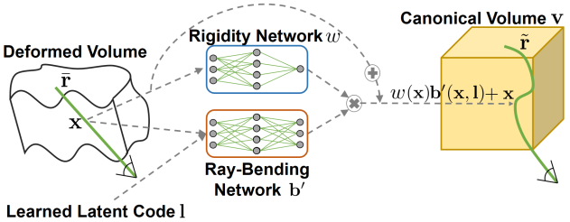
The ray bending MLP disentangles the geometry of the scene from the scene deformations. The disentanglement is an underconstrained problem, which we tackle with further innovations. Our method assigns a rigidity score to every point in the canonical volume, which allows for the deformations to not affect the static regions in the scene. This rigidity component is jointly learned without any direct supervision. We also introduce multiple regularizers as additional soft-constraints: A regularizer on the deformation magnitude of the visible deformations encourages only sparse deformations of the volume, and thus helps to constrain the canonical volume. An additional divergence regularizer preserves the local shape, thereby constraining the representation of hidden (partially occluded) regions that are not visible throughout the full video.
Our results show high-fidelity reconstruction and novel view synthesis for a wide range of non-rigid scenes. Fig. 2 contains an overview of our method. To summarize, our main technical contributions are as follows:
-
•
A free viewpoint rendering method, NR-NeRF, that only requires a monocular video of the dynamic scene (Sec. 3). The spatio-temporal camera trajectory for test-time novel view synthesis can differ significantly from the trajectory of the input video. Moreover, we can extract dense correspondences relating arbitrary (input or novel) frames.
-
•
A rigidity network which can segment the scene into non-rigid foreground and rigid background without being directly supervised (Sec. 3.2).
-
•
Regularizers on the estimated deformations which constrain the problem by encouraging small volume preserving deformations (Sec. 3.3).
-
•
Several extensions for handling of view dependence and multi-view data, and applications of our technique for simple scene editing (Secs. 3).
We compare NR-NeRF to several methods for neural novel view rendering (Sec. 4). See our supplementary video for visualizations and Sec. S.10 for a discussion.
2 Related Work
4D Reconstruction and Novel Viewpoint Rendering.
Early methods for image-based novel and free-viewpoint rendering combined traditional concepts of multi-view camera geometry, explicit vision-based 3D shape and appearance reconstruction, and classical computer graphics or image-based rendering. These methods are based on light fields [35, 19, 4], multi-view stereo to capture dense depth maps [99], layered depth images [70], or representations using 3D point clouds [1, 40, 67], meshes [44, 86] or surfels [62, 7, 88] for dynamic scenes. Passive geometry capture often leads to artifacts in scenes with severe occlusions and view-dependent appearance. Also, capturing temporally coherent representations in this way is challenging.
More recently, the combination of multi-view stereo with fusion algorithms integrating implicit geometry over short time windows lead to improved results and short-term temporal coherence [10, 55, 22]. By using active depth cameras and such fusion-type reconstruction, dynamic scene capture and novel viewpoint rendering from a low number of cameras or a single camera were shown [96, 81, 25, 97]. Several algorithms use variants of shape-from-silhouette to approximate real scene geometry, such as visual hull reconstruction or visual hulls improved via multi-view photo-consistency in [34, 78]. While reconstruction is fast and feasible with fewer cameras, the coarse approximate geometry introduces rendering artifacts, and the reconstruction is usually limited to the separable foreground. Accurate and temporally coherent geometry is hard to capture in this way [5, 6]. Some approaches use 3D templates and combine vision-based reconstruction with appearance modelling to enable free-viewpoint video relighting, e.g., by estimating reflectance models under general lighting or under controlled light stage illumination [83, 36, 49, 21].
The progress in RGB-D sensors has enabled depth map capture from a single camera. Such sensors can been used for 3D reconstruction and completion of rigid environments [52] and non-rigid objects [103, 51, 28, 75]. Other method classes allow capturing deformable geometry from sets of monocular views. Dense non-rigid structure from motion requires dense point tracks over input images, which are then factorized into camera poses and non-rigid 3D states per view [17, 33, 72]. The correspondences are usually obtained with dense optical flow methods, which makes them prone to occlusions and inaccuracies, and which can have a detrimental effect on the reconstructions. Monocular template-based methods do not assume dense matches and rely on a known 3D state of a deformable object (a 3D template), which is then tracked across time [61, 53, 95, 92], or a training dataset with multiple object states [18, 85]. Obtaining templates for complex objects and scenes is often non-trivial and requires specialized setups.
In contrast, our approach avoids explicit image-based 3D reconstruction. Moreover, we support arbitrary backgrounds whereas the discussed methods for monocular 3D reconstruction of deformable objects ignore it. Our approach enables free-viewpoint rendering of general deformable scenes with multiple objects and complex deformations with high visual fidelity, and yet does not rely on templates, 2D correspondences and multi-view setups.
Neural Scene Representations and Neural Rendering. An emerging algorithm class uses neural networks to augment or replace established graphics and vision concepts for reconstruction and novel-view rendering. Most recent work is designed for static scenes [24, 13, 54, 45, 14, 73, 74, 47, 65]; methods for dynamic scenes are in their infancy.
Several approaches address related problems to ours, such as generating images of humans in new poses [2, 42, 50, 66] or body reenactment from monocular videos [8]. Other methods combine explicit dynamic scene reconstruction and traditional graphics rendering with neural re-rendering [43, 30, 29, 94]. Shysheya et al. [71] proposed a neural rendering approach for human avatars with texture warping. Zhu et al. [102] leverage geometric constraints and optical flow for synthesizing novel views of humans from a single image. Thies et al. [84] combine neural textures with the classical graphics pipeline for novel view synthesis of static objects and monocular video re-rendering. Neural Volumes [41] learn object models which can be animated and rendered from novel views, given multi-view video data. In contrast to all these methods, we require only a set of monocular views of a non-rigid scene as input and are able to render the scene from novel views.
Non-Peer-Reviewed Reports. Since the intersection of neural scene representations and volumetric rendering has recently become a very active area of research with quickly evolving progress, several methods for dynamic settings have been proposed concurrently to ours. We mention them only for completeness since they are not peer-reviewed and thus do not constitute prior work. Some methods extend neural radiance fields to deforming faces [87, 16, 15, 64]. Others focus on moving human bodies [89, 60, 79] or more general objects [63, 38, 90, 58, 11, 37]. Our method differs from these by tackling general, real-world dynamic scenes from monocular RGB observations and camera parameters only, without using any other auxiliary method to estimate, for example, optical flow or depth.
3 Method
Our Non-Rigid Neural Radiance Field (NR-NeRF) approach takes as input a set of RGB images of a non-rigid scene and their extrinsics and intrinsics . NF-NeRF then finds a single canonical neural radiance volume that can be deformed via ray bending to correctly render each . Specifically, we collect appearance and geometry information in the static canonical volume parametrized by weights . We model deformations by bending the straight rays sent out by a camera to obtain a deformed rendering of . This ray bending is implemented as a ray bending MLP with weights . It maps, conditioned on the current deformation, 3D points (e.g., sampled from the straight rays) to 3D positions in . The deformation conditioning takes the form of auto-decoded latent codes for each image .
3.1 Background: Neural Radiance Fields
We first recap NeRF [46] for rigid scenes. NeRF renders a 3D volume into an image by accumulating color, weighted by accumulated transmittance and density, along camera rays. The 3D volume is parametrized by an MLP that regresses an RGB color and an opacity for a point on a ray with direction .
Consider a pixel of an image . For a pinhole camera, the associated ray can be calculated using , and , which yield the ray origin and ray direction . We can then integrate along the ray from the near plane to the far plane of the camera frustum to obtain the final color at :
| (1) |
with being the accumulated transmittance along the ray from up to . In practice, the integrals are approximated by discrete samples along the ray. NeRF employs a coarse volume with network weights and a fine volume with network weights . Both volumes have the same architecture, but do not share weights: . When rendering a ray, is accessed first at uniformly distributed samples along the ray. These coarse samples are used to estimate the transmittance distribution, from which fine samples are sampled. is then evaluated at the combined set of coarse and fine sample points. We refer to the original paper for more details.
Adaptations for NR-NeRF. We assume Lambertian materials and thus remove the view-dependent layers of rigid NeRF, i.e., we set . Since each image corresponds to a different deformation of the volume in our non-rigid setting, we also learn a latent code for each time step, which is then used as input for the ray bending network which parameterizes scene deformations. The weights of this network and the latent codes are shared between and .
3.2 Deformation Model
The original NeRF method [46] assumes rigidity and cannot handle non-rigid scenes. A naïve approach to modeling deformations in the NeRF framework would be to condition the volume on the deformation (e.g., by conditioning it on time or a deformation latent code). We explore the latter option in the experiments in Sec. S.7. As we will show, apart from not providing hard correspondences, this naïve approach only leads to satisfying results when reconstructing the input camera path, but gives implausible results for novel view synthesis. Instead, we explicitly model the consistency of geometry and appearance across time by disentangling them from the deformation.
We accumulate geometry and appearance from all frames into a single, non-deforming canonical volume. We employ general space warping (or ray bending) on top of the static canonical volume to model non-rigid deformations.
For an input image at training time, we want to render the canonical volume such that the image is reproduced. To that end, we need to un-do the deformation of the specific time step by mapping the camera rays to the deformation-independent canonical volume. We first send out straight rays from the input camera. To account for the deformation, we then bend the straight rays such that sampling and subsequently rendering the canonical volume along the bent rays yields . We choose a very unrestricted parametrization of the ray bending, namely an MLP.
Specifically, we implement ray bending as a ray bending network . For a point , for example lying on a straight ray, the network regresses an offset under a deformation represented by . The offset is then added to , thus bending the ray. Finally, we pass the new, bent ray point to the canonical volume, that is: . Note that is not conditioned on , which leads to the disentanglement of deformation ( and ) from geometry and appearance (). We denote the bent version of the straight ray as .
Rigidity Network. However, we find that rigid parts of the scene are insufficiently constrained by this formulation. We reformulate as the product of a raw offset and a rigidity mask , i.e., . For rigid objects, we want to prevent deformations and hence desire , while for non-rigid objects, we want . This makes it easier for to focus on the non-rigid parts of the scene, which change over time, since rigid parts can get masked out by the rigidity network , which is jointly trained. Because the rigidity network is not conditioned on the latent code , it is forced to share knowledge about the rigidity of regions in the scene across time steps, which also ensures that parts of the rigid background that can be unregularized at certain time steps are nonetheless reconstructed at all time steps without any deformation.
3.3 Losses
With the architecture specified, we next optimize all parameters (, , ) jointly. We optimize the network weights as usual but auto-decode the latent codes [80, 57].
Notation. For ease of presentation, we consider a single time step and a single straight ray with coarse ray points for a set of uniformly sampled and fine ray points for a set of importance-sampled . For a latent code , the bent ray gives and . The actual training uses a batch of randomly chosen rays from the training images.
Reconstruction Loss. We adapt the data term from NeRF to our non-rigid setting as follows:
| (2) |
where is the ground-truth color of the pixel and is the estimated ray color on the set of discrete ray points.
While this reconstruction loss yields satisfactory results along the space-time camera trajectory of the input recording, we show later in Sec. 4.2 that it leads to undesirable renderings for novel views. We thus find it necessary to regularize the bending of rays with further priors.
Offsets Loss. We regularize the offsets with a loss on their magnitude. Since we want visually unoccupied space (i.e., air) to be compressible and not hinder the optimization, we weigh the loss at each point by its opacity. However, this would still apply a high weight to completely occluded points along the ray, which leads to artifacts when rendering novel views. We thus additionally weigh by transmittance:
| (3) |
where we weigh each point by transmittance and occupancy . We do not back-propagate into .
However, as we show in Sec. 4, we find that applying the offsets loss to the masked offsets leads to an unstable background in novel views. We hypothesize that this is due to the multiplicative ambiguity between unmasked offsets and rigidity mask. We find that applying the loss to the regressed rigidity mask and raw offsets separately works better:
| (4) |
where we penalize instead of . The exponent of the first term is a tweak to get two desirable properties that neither an nor an loss fulfills: For non-rigid objects ( closer to ), it becomes an loss, which has two advantages: (1) the gradient is independent of the magnitude of the offset, so unlike with an loss, small and large offsets/motions are treated equally, and (2) relative to an loss, it encourages sparsity in the offsets field, which fits our scenes. For rigid objects ( closer to ), it becomes an loss, which tampers off in its gradient magnitude as the offset magnitude approaches 0, preventing noisy gradients that an loss has for the tiny offsets of rigid objects.
Divergence Loss. Since the offsets loss only constrains visible areas, we introduce additional regularization of hidden areas. Inspired by local, isometric shape preservation from computer graphics, like as-rigid-as-possible regularization for surfaces [77, 27] or volume preservation for volumes [75], we seek to preserve the local shape after deformation. To that end, we propose to regularize the absolute value of the divergence of the offsets field. The Helmholtz decomposition [3] allows to split any twice-differentiable 3D vector field on a bounded domain into a sum of a rotation-free and a divergence-free vector fields. Thus, by penalizing the divergence, we encourage the vector field to be composed primarily of translations and rotations, effectively preserving volume. The divergence loss is:
| (5) |
where we do not back-propagate into , and we take the divergence of w.r.t. the position .
We employ FFJORD’s [20] fast, unbiased divergence estimation, which is three times less computationally expensive than an exact computation. The divergence is defined as:
| (6) |
where is the -th component of , is the trace operator, and is the Jacobian matrix. Naïvely computing the divergence with PyTorch’s automatic differentiation requires three backward passes, one for each term of the sum. Instead, the authors of FFJORD [20] use Hutchinson’s trace estimator [26]:
| (7) |
Here, is Gaussian-distributed. The single-sample Monte-Carlo estimator implied by this expectation can be computed with a single backward pass.
Full Loss. We combine all losses to obtain the full loss:
| (8) |
where the weights , , and are scene-specific since we consider a variety of non-rigid scene types. Our implementation uses the structure-from-motion method COLMAP [67] to estimate the camera parameters. For further training and implementation details, we refer to the supplemental material. We will release our source code.
4 Results
We present qualitative results of our method, including rigidity scores and correspondences, by rendering into input and novel spatio-temporal views in Sec. 4.1.Turning to the inner workings, Sec. 4.2 investigates the crucial design choices we made to improve novel view quality. We conclude the evaluation of our approach in Sec. S.7 by comparing to prior work and a baseline approach. Finally, we show simple scene-editing results in Sec. S.9. In the supplemental material, we provide information on data capture and show extensions to multi-view data and view-dependent effects.
 |
 |
 |
|
Input |
 |
 |
Color |
 |
 |
||
|
Rigidity |
 |
 |
Correspondences |
 |
 |
4.1 Qualitative Results
We present qualitative results of NR-NeRF by rendering the scene from input and novel spatio-temporal views. We also visualize the additional outputs of our method.
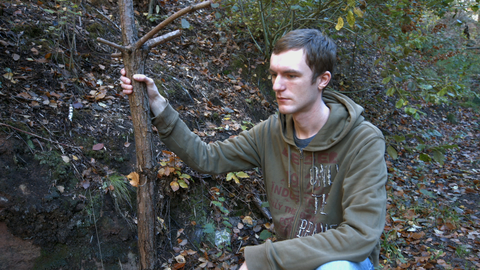
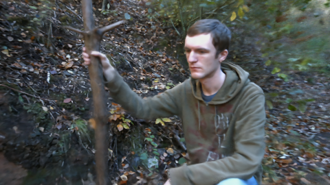
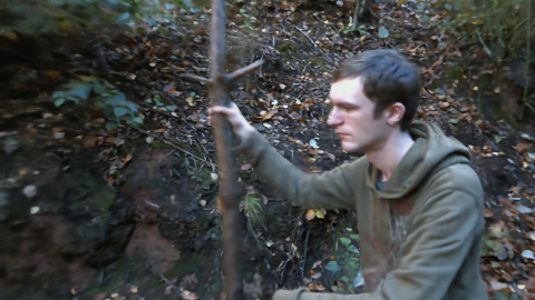
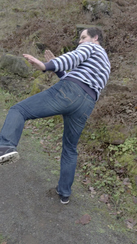
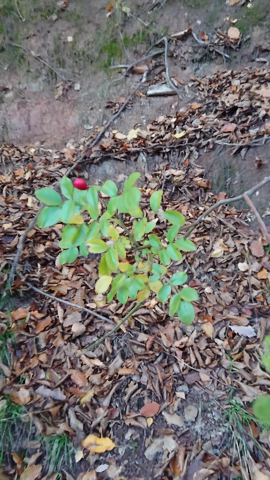
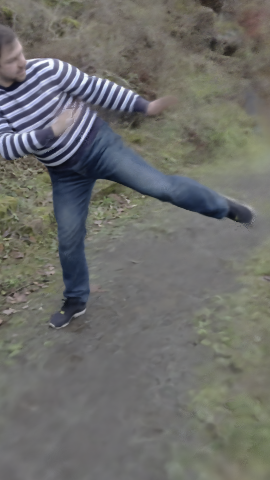
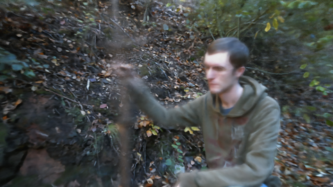
Input Reconstruction and Novel View Synthesis. Fig. 3 shows examples of input reconstruction and novel view synthesis with NR-NeRF. As the center column shows, the input is reconstructed faithfully. This enables high-quality novel view synthesis, example results can be found in the third column. We can freely move the camera in areas around the original camera paths and specify the time step.
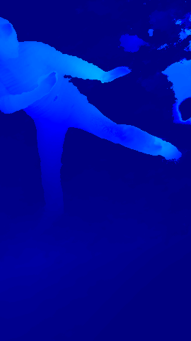
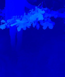
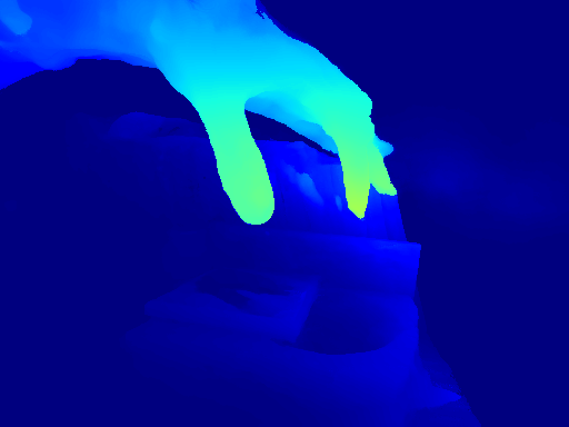
Rigidity. NR-NeRF estimates rigidity scores without supervision to improve background stability in novel-view renderings. We show examples in Fig. 4 and find that the background is consistently scored as highly rigid while foreground is correctly estimated to be rather non-rigid.
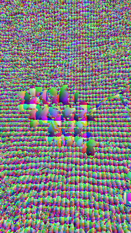
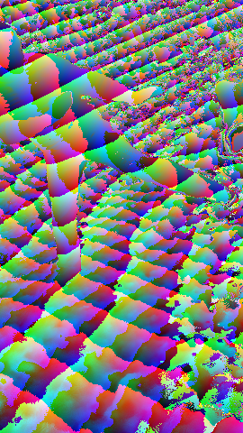
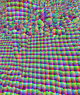
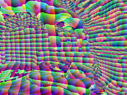
Correspondences. Another side effect of our proposed approach is the ability to estimate consistent dense 3D correspondences into the canonical model across different camera views and time steps. Fig. 4 shows examples.
4.2 Ablation Study
After this look at the outputs of NR-NeRF, we now turn to its internal workings. Specifically, since we aim for convincing novel-view renderings, we take a closer look at the impact of some of our design choices on the foreground and background stability of our novel-view results.
Setup. We investigate the necessity of all regularization losses by removing each loss individually and all of them at once. Next, we remove the rigidity network to see the impact on background stability. Finally, we determine whether applying the offsets loss separately on both the regressed rigidity and the unmasked offsets, i.e., in our method, or directly on the masked offsets, , works better.
Results. We find that is crucial for stable deformations of the non-rigid objects in the foreground, see Fig. 5.
 |
 |
 |
| Without | No regularization | Ours |
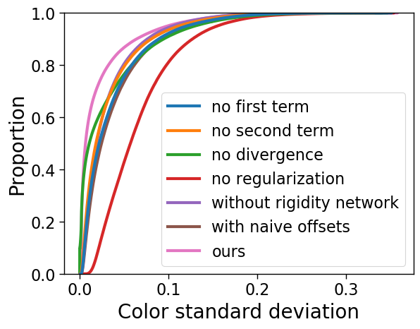
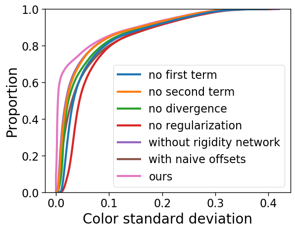
On the other side, the interplay of all of the remaining design choices is necessary to stabilize the rigid background as Fig. 6 shows. The supplemental video contains video examples that highlight the instability in these cases.
| a) | |||
 |
 |
||
| Left scene | Right scene | ||
| b) | |||
| Ours | |||
| . | |||
| No first term of offsets loss | No second term of offsets loss | ||
| . | |||
| Without divergence loss | Without any regularization loss | ||
| . | |||
| Without rigidity network | With | ||
| . | |||
4.3 Comparisons
Having only considered our method in isolation so far, we next compare NR-NeRF to prior work and a baseline. In this section, we split the images into training and test sets by partitioning the temporally-ordered images into consecutive blocks of length 16 each, with the first twelve for the training set and the remaining four for the test set.
Prior Work and Baseline. We start with the trivial baseline of rigid NeRF [46], which cannot handle dynamic scenes. We consider two variants: view-dependent rigid NeRF, as in the original method [46], and view-independent rigid NeRF, where we remove the view-direction conditioning. We next introduce naïve NR-NeRF, which adds naïve support for dynamic scenes to rigid NeRF: We condition the neural radiance fields volume on the latent code , i.e., . For test images , we backpropagate gradients into the corresponding latent code . We do the same for NR-NeRF in order to optimize for the test latent codes. Note that test images solely influence test latent codes, as is typical for auto-decoding [57]. Finally, we compare to Neural Volumes [41], for which we use the official code release. We consider two variants: (1) as in [41], the geometry and appearance template is conditioned on the latent code (NV), and (2) the geometry and appearance template are independent of the latent code (modified NV).
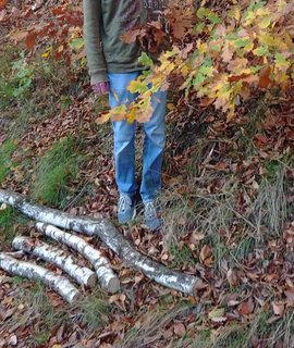
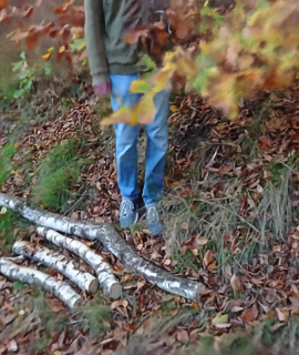
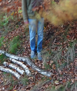
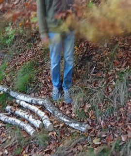
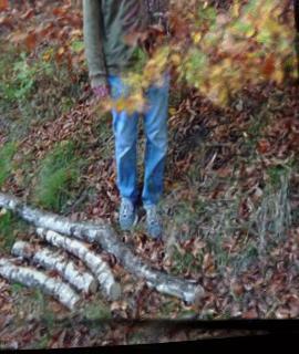
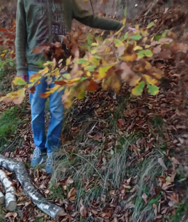
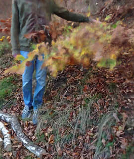
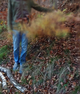
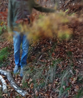
Input Reconstruction. We first consider input reconstruction quality on the training set to verify the plausibility of the learned representations. See Fig. 7. We find that naïve NR-NeRF and both variants of Neural Volumes perform very well on this task, similar to our method. However, rigid NeRF’s not accounting for deformations leads to blur.
Novel View Synthesis. We next evaluate novel-view performance qualitatively and quantitatively on the test sets. Fig. 7 contains novel-view results of all methods. Both versions of Neural Volumes give implausible results that are in some cases only barely recognizable. The two rigid NeRF variants show blurry, static results similar to the training reconstruction results earlier. While the still images in Fig. 7 show some undesirable artifacts like blurrier or less stable results compared to ours, we refer to the supplemental video to see naïve NeRF’s temporal inconsistencies , especially on spatio-temporal trajectories different from the input.
| Input | Ours | Naïve NR-NeRF | Rigid NeRF | Rigid NeRF | Neural Volumes | Neural Volumes |
|---|---|---|---|---|---|---|
| (view-dep.) | (not view-dep.) | (modified) | ||||
 |
 |
 |
 |
 |
 |
 |
 |
 |
 |
 |
 |
 |
After the qualitative overview, we now evaluate the novel-view results of the methods considered quantitatively. We use the same three metrics as NeRF [46]. We use PSNR and SSIM [101] as conventional metrics for image similarity, where higher is better. In addition, we use a learned perceptual metric, LPIPS [100], where lower is better. Tab. 1 contains the quantitative results. Our method obtains the best SSIM and LPIPS scores, and the second-best PSNR after naïve NR-NeRF. As we saw in the input reconstruction results, naïve NR-NeRF is competitive for settings that are close to the input spatio-temporal trajectory, as is the case for our test sets. We, therefore, next evaluate more challenging novel view scenarios with a spatio-temporal trajectory significantly different from the input. Since we do not have access to ground-truth novel view data, we focus on background stability for a spatially fixed camera.
| Ours | Naïve | Rigid | Rigid | NV | NV | ||
|---|---|---|---|---|---|---|---|
| (cond.) | (no cond.) | (mod.) | |||||
| PSNR | 22.24 | 21.88 | 14.13 | 14.10 | |||
| SSIM | 0.662 | 0.659 | 0.259 | 0.263 | |||
| LPIPS | 0.309 | 0.313 | 0.580 | 0.583 |
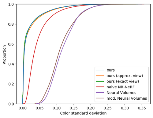
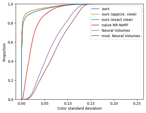
Background Stability. While a moving camera during rendering can obfuscate background instability, we found that stabilizing the background for fixed novel-view renderings matters for perceptual fidelity but is difficult to achieve. We thus quantitatively evaluate on this challenging task here. In Fig. 8, we compare the background stability of our method, naïve NR-NeRF, and the Neural Volumes variants. We exclude rigid NeRF since it is static by design. We find that our method leads to significantly more stable background synthesis than the other methods, and we refer to the supplemental material for further results.
| Ours | Naïve NR-NeRF | ||
| Neural Volumes | Neural Volumes (modified) | ||
4.4 Simple Scene Editing
We can manipulate the learned model in several simple ways: foreground removal, temporal super-sampling, deformation exaggeration and dampening, and forced background stabilization. We discuss foreground removal here and the other editing tasks in the supplemental material due to space constraints.
Our representation enables us to remove a potentially occluding non-rigid object from the foreground, leaving only the unoccluded background. Assuming the rigidity network assigns higher scores to non-rigid objects than to rigid (background) objects, we can threshold them at test time to segment the canonical volume into rigid and non-rigid parts. We can then set the non-rigid part transparent, see Fig. 9.
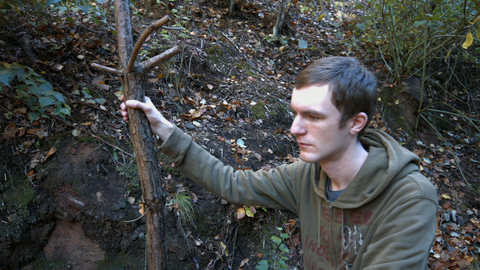
5 Limitations
For simplicity, the discrete integration along the bent ray uses the interval lengths given by the straight ray. As we build on NeRF, our method is similarly slow. All else being equal, ray bending increases runtime by about 20%. However, due to fewer rays and points sampled, we train for 6 hours. We can thus train multiple NR-NeRFs (to find appropriate loss weights) in a time similar to other NeRF-based methods [46]. Neural Sparse Voxel Fields [39] are a promising direction to speed up NeRF-like methods. The background needs to be fairly close to the foreground, an issue we “inherit” from NeRF and which could be addressed similarly to NeRF++ [98]. Since we use a deformation model that does not go from the canonical space to the deformed space, we cannot obtain exact correspondences between images captured at different time steps, but instead need to use a nearest neighbor approximation. We do not account for appearance changes that are due to deformation or lighting changes. For example, temporally changing shadowing in the input images is an issue. Foreground removal can fail if a part of the foreground is entirely static. Rendering parts of the scene barely or not at all observed in the training data would not lead to realistic results. Motion blur in input images is not modeled and would lead to artifacts. The background needs to be static and dominant enough for structure-from-motion [67] to estimate correct extrinsics. Since our problem is severely under-constrained, we employ strong regularization, which leads to a trade-off between sharpness and stability on some scenes.
6 Conclusion
We presented a method for free viewpoint rendering of a dynamic scene using just a monocular video as input. Several high-quality reconstruction and novel view synthesis results of general dynamic scenes, as well as unsupervised, yet plausible rigidity scores and dense 3D correspondences demonstrate the capabilities of the proposed method. Our results suggest that space warping in the form of ray bending is a promising deformation model for volumetric representations like NeRF. Furthermore, we have demonstrated that background instability, a problem also noted by concurrent work [58], can be mitigated in an unsupervised fashion by learning a rigidity mask. The extensions to multi-view data and view dependence invite future work on more constrained settings for higher quality. Although rather rudimentary, we have shown that NR-NeRF enables several scene-editing tasks, and we look forward to further work in the direction of editable neural representations.
Acknowledgements. All data capture and evaluation was done at MPII and Volucap. We thank Volucap for providing the multi-view data. Research conducted by Ayush Tewari, Vladislav Golyanik and Christian Theobalt at MPII was supported in part by the ERC Consolidator Grant 4DReply (770784). This work was also supported by a Facebook Reality Labs research grant.
NR-NeRF — Supplemental Material
Overview
We provide further illustrations of the loss function in Sec. S.1. We discuss a number of training details in Sec. S.2. Next, we provide some implementation details in Sec. S.3. In Sec. S.4, we describe the capture of our data. Sec. S.5 contains details on how we visualize the additional output modalities of our method and some more results. We show an additional result of our ablation study in Sec. S.6. We provide more details on the experimental settings of our comparisons and some additional results in Sec. S.7. Then in Sec. S.8, we present the extensions to multi-view data and view-dependent effects mentioned in the main paper. Sec. S.9 contains the scene editing tasks mentioned in the main paper. Sec. S.10 contains a limitation example of our method. Finally, Sec. S.11 contains some preliminary qualitative comparisons to a concurrent, non-peer-reviewed work.
S.1 Loss Illustration
Fig. S.1 illustrates in 2D.

S.2 Training Details
While the network weights are optimized as usual, the latent codes are auto-decoded, i.e., they are treated as free variables that are directly optimized for, similar to network weights, instead of being regressed. This is based on the auto-decoding framework used in DeepSDF and earlier works [80, 57].
We initialize to zero vectors. For implementing the radiance field, we use the same architecture as in NeRF [46]. The ray bending network is a 5-layer MLP with 64 hidden dimensions and ReLU activations, the last layer of which is initialized with all weights set to zero. The rigidity network is a 3-layer MLP with 32 hidden dimensions and ReLU activations, with the last layer initialized to zeros. The output of the last layer of the rigidity network is passed though a activation function and then shifted and rescaled to lie in . We train usually for 200k iterations with a batch of 1k randomly sampled rays. At training and at test time, we use 64 coarse and 64 fine samples per ray in most cases. We use ADAM [31] and exponentially decay the learning rate to 10% from the initial over 250k iterations. For dark scenes, we found it necessary to introduce a warm-up phase that linearly increases the learning rate starting from th of its original value over 1000 iterations. The latent codes are of the dimension 32. We train between six and seven hours on a single Quadro RTX 8000.
Since we consider a variety of types of non-rigid objects/scenes and deformations, we find it necessary to use scene-specific weights for each loss term. We have found the following ranges to be sufficient for a wide range of scenarios: lies in and typically is , lies in and typically is , and lies in and typically is or . In our experience, NR-NeRF is fairly insensitive to . Rather rigid objects benefit from higher , while fairly non-rigid objects need lower . Finally, we increase whenever we find the background to be unstable. We start the training with each weight set to th of its value, and then exponentially increase it until it reaches its full value at the end of training.
S.3 Implementation Details
Our code is based on a faithful PyTorch [59] port [93] of the official Tensorflow NeRF code [46]. We use the official FFJORD implementation [20] to estimate Eq. 5 from the main paper. If the camera extrinsics and intrinsics are not given, we estimate them using the Structure-from-Motion (SfM) implementation of COLMAP [68, 69]. We find COLMAP to be quite robust to non-rigid ‘outliers’. As we are interested in estimating smooth deformations, we only apply positional encoding to the input of the canonical NeRF volume, not to the input of the ray bending network. We will make our source code available.
S.4 Data
We show results on a variety of scenes recorded with three different cameras: the Kinect Azure, a Blackmagic, and a phone camera. Since the RGB camera of the Kinect Azure exhibits strong radial distortions along the image border, we use the manufacturer-provided intrinsics and distortion parameters to undistort the recorded RGB images beforehand. We extract frames at 5 fps from the recordings, such that scenes usually consist of 80 to 300 images, at resolutions of (Blackmagic, and Sony XZ2) or (Kinect Azure).
S.5 Output Modalities
S.5.1 Visualizations
Rigidity Scores
In order to visualize the estimated rigidity, we need to determine the rigidity of the ray associated with a pixel. We choose to define the rigidity of such a ray as the rigidity of the point closest to an accumulated weight of 0.5, i.e., closest to the median. In practice, this usually gives us the rigidity at the first visible surface along the ray.
Correspondences
To visualize correspondences, we treat the canonical volume as an RGB cube, i.e., we treat the xyz coordinate in canonical space as an RGB color. Since this would result in very smooth colors, we split the canonical volume into a voxel grid of RGB cubes beforehand. We pick the ray point that determines the pixel color similar to the rigidity visualization.
S.5.2 More Results
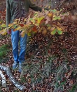
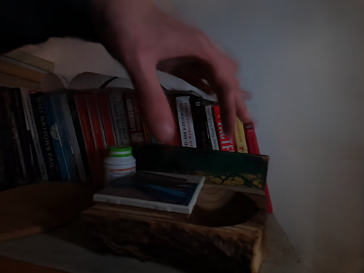
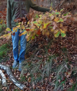
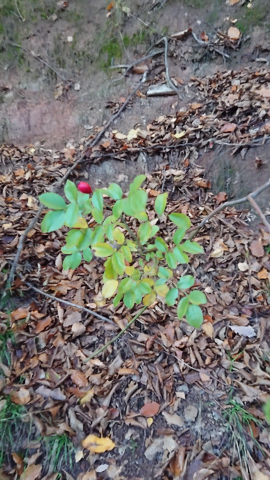
See Fig. S.2 for more results of the output modalities of NR-NeRF.
Canonical Volume
Since the canonical volume is not supervised directly, it is conceivable that it could have baked-in deformations. The last row of Fig. S.2 contains renderings of the canonical volume without any ray bending applied. The canonical volume is a plausible state of the scene and does not show baked-in deformations. We thus find it to be sufficient to bias the optimization towards a desirable canonical volume by initializing the ray bending network to an identity map and by our regularization losses.
|
Input |
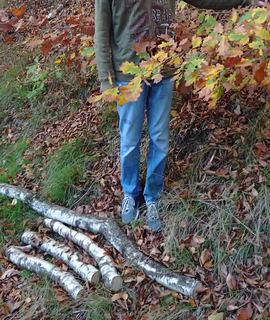 |
 |
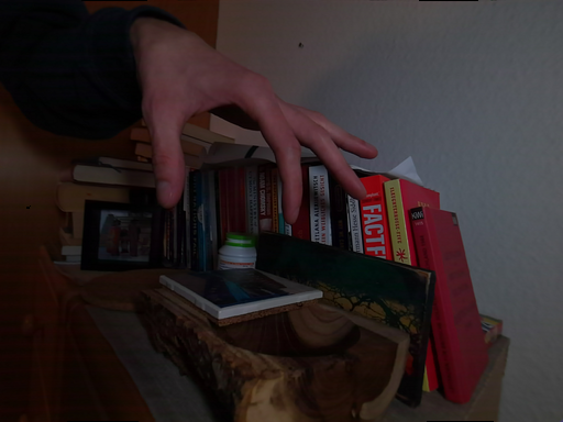 |
 |
|
|
Color |
 |
 |
 |
 |
|
|
Rigidity |
 |
 |
 |
 |
|
|
Correspondences |
 |
 |
 |
 |
|
|
Canonical Volume |
 |
 |
 |
 |
|
| . |
S.6 Ablation Study
Fig. S.3 contains an additional ablation study result that demonstrates the importance of the divergence regularization for foreground stability.
 |
 |
 |
| Without | No regularization | Ours |
S.7 Comparisons
In this section, we provide more details on the experimental settings of the comparisons.
S.7.1 Prior Work and Baseline
We start with the trivial baseline of rigid NeRF [46], which cannot handle dynamic scenes. We consider two variants: view-dependent rigid NeRF, as in the original method [46], and view-independent rigid NeRF, where we remove the view-direction conditioning.
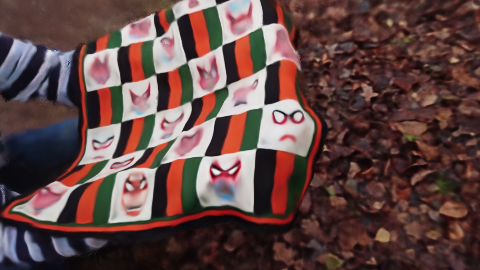
We next introduce naïve NR-NeRF, which adds naïve support for dynamic scenes to rigid NeRF: We condition the neural radiance fields volume on the latent code. Thus, for latent code , we have . This allows the neural radiance fields volume to output time-varying color and occupancy. Unlike NR-NeRF’s ray bending, naïve NR-NeRF does not have an explicit, separate deformation model. Instead, the volume needs to account for appearance, geometry and deformation at once. Note that for test images , we do backpropagate gradients into the corresponding latent code .
Finally, we compare to Neural Volumes [41], for which we use the official code release. We use the standard settings as a starting point, but set the number of training iterations to , which leads to a training time of about two days on an RTX8000 GPU. Neural Volumes uses an image encoder to regress a latent code that conditions the geometry, appearance and deformation regression on the current time step. Since this design assumes a multi-view setup, we need to adapt it to our monocular setting. Instead of picking three fixed camera views that are always input into the encoder, we input the single image of the current time step. In particular, at test time, we input the test image. Since we do not have access to a background image, we set the estimated background image to an all-black image. We furthermore consider two variations: (1) following the original Neural Volumes method, the geometry and appearance template is conditioned on the latent code (NV), and (2) the geometry and appearance template is independent of the latent code (modified NV). In the latter case, the latent code only conditions the warp field, which is similar to our method.
S.7.2 Training/Test Split
For quantitative evaluation, we require a test set. In the comparison section, we split the images into training and test images by partitioning the temporally-ordered images into consecutive blocks, each of length 16. The first twelve images of each block are used as training data, while the remaining four are used for testing. In our setting, test images still require corresponding latent codes to represent the deformations. Therefore, we treat test images like training images except that we do not backpropagate into the canonical volume or the ray bending network. However, we do use gradients from test images to optimize the corresponding latent codes. (Note that test images solely influence test latent codes, as is typical for auto-decoding [57]. 111The only tweak we add is that we align the optimization landscapes of the training and test latent codes by optimizing the test latent codes jointly with the training latent codes during training. This does not lead to any information leakage from the test images to any component except for the test latent codes.) All other results shown in this paper, outside of the comparisons, treat all images as training images since we train scene-specific networks. Furthermore, qualitative baseline results in the supplemental video show both training and test time steps.
S.7.3 Additional Results
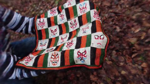
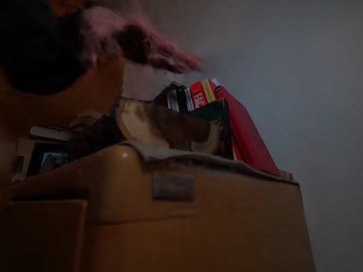
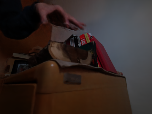
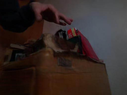
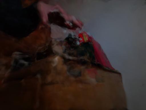
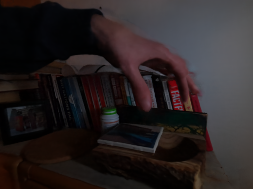
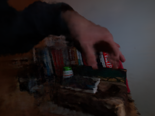
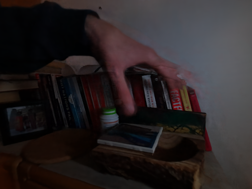
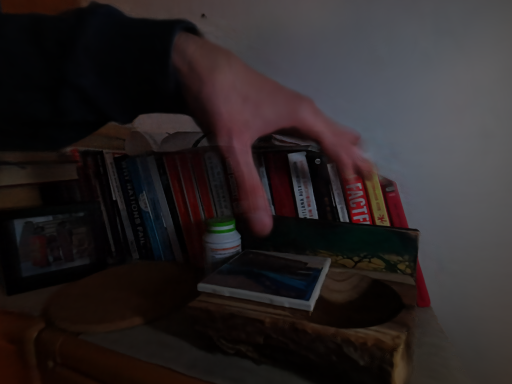
See Fig. S.4 for more qualitative results and Fig. S.7 for quantitative results on background stability under novel views.
| Input | Ours | Naïve NR-NeRF | Rigid NeRF | Rigid NeRF | Neural Volumes | Neural Volumes |
|---|---|---|---|---|---|---|
| (view-dep.) | (not view-dep.) | (modified) | ||||
 |
 |
 |
 |
 |
 |
 |
 |
 |
 |
 |
 |
 |
|
 |
 |
 |
 |
 |
 |
 |
 |
 |
 |
 |
 |
 |
|
 |
 |
 |
 |
 |
 |
 |
 |
 |
 |
 |
 |
 |
S.8 Extensions
As mentioned in Sec. 4 from the main paper, we can extend our approach easily to work with multi-view data and view-dependent effects.
S.8.1 Multi-View Data
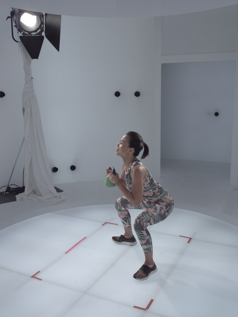
Our approach naturally handles multi-view data. Although we mainly work with monocular data, we can use multi-view data to investigate the upper quality bound of our approach under ideal real-world conditions.
Method
Instead of each image having its own time step and hence latent code, images taken at the same time step share the same latent code. This ensures that the canonical volume deforms consistently within each time step.
Data and Settings
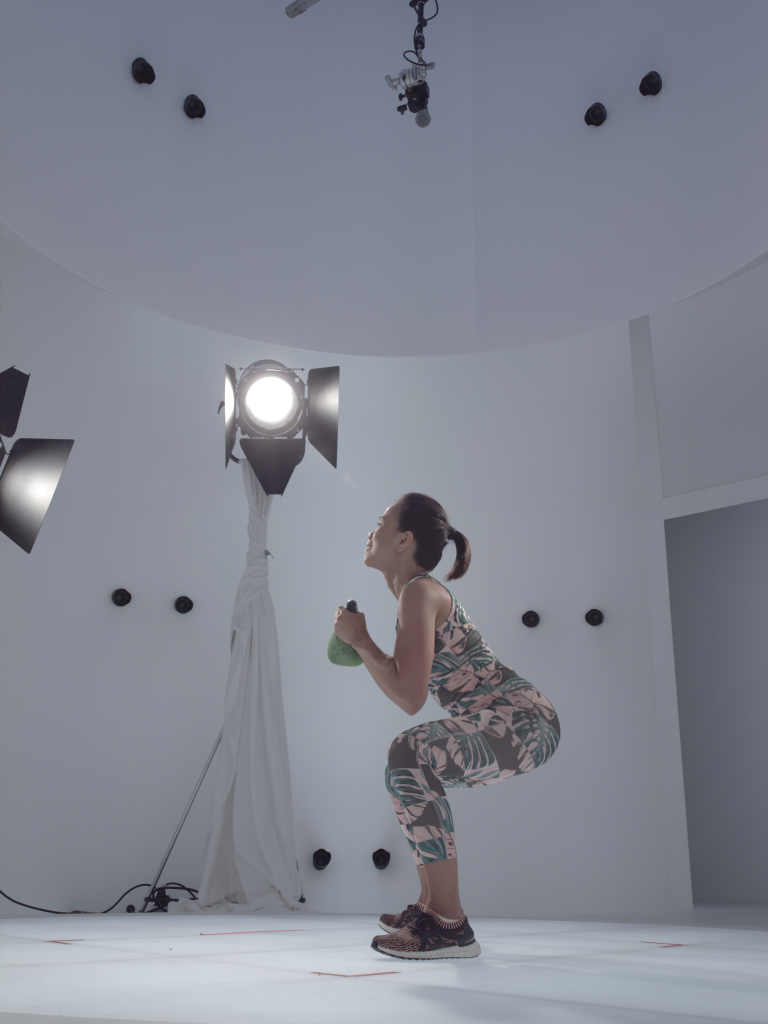
We use a multi-view dataset that has 16 camera pairs evenly distributed around the scene, which sufficiently constrains the optimization such that we find the training to not need any regularization losses. We train at the original resolution of for 2 million training iterations with 4096 rays per batch and 256 coarse and 128 fine samples. These highest-quality settings lead to a training time of 11 days on 4 RTX8000 GPUs, and a rendering time of about 10 minutes per frame on the same hardware.
Results
See Fig. S.5 and the supplemental video for results on five consecutive time steps.
S.8.2 View Dependence
We can optionally add view-dependent effects, like specularities, into our model.
Method
Determining the view direction or ray direction is not as trivial as for the straight rays. Instead, we need to calculate the direction in which the bent ray passes through a point in the canonical volume. We consider two options of doing so: exact and slower, or approximate and faster.
Exact: We obtain the direction of the bent ray at a point via the chain rule as , where is the Jacobian and is the direction of the straight ray. We compute via three backward passes (one for each output dimension), which is computationally expensive.
Approximate: To reduce computation, we can approximate the direction at the ray sample via finite differences as the normalized difference vector between the current point and the previous point along the bent ray (which is closer to the camera).
Results
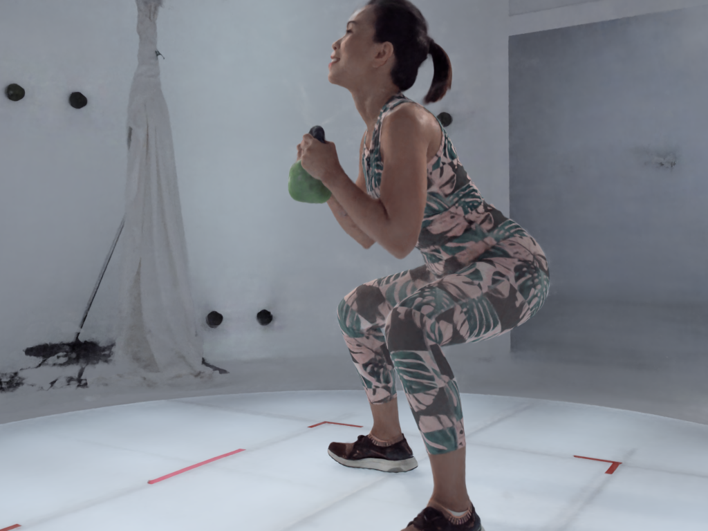
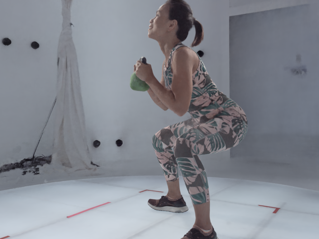
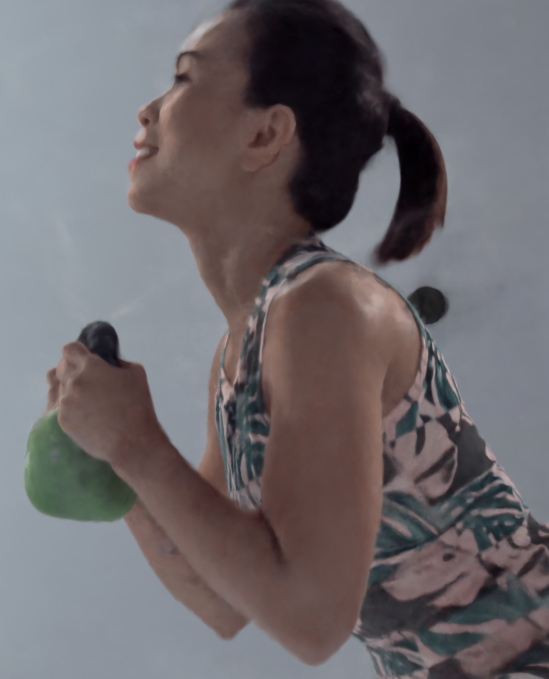
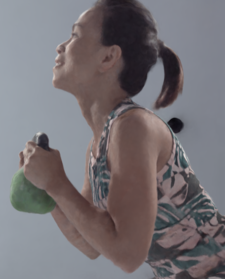
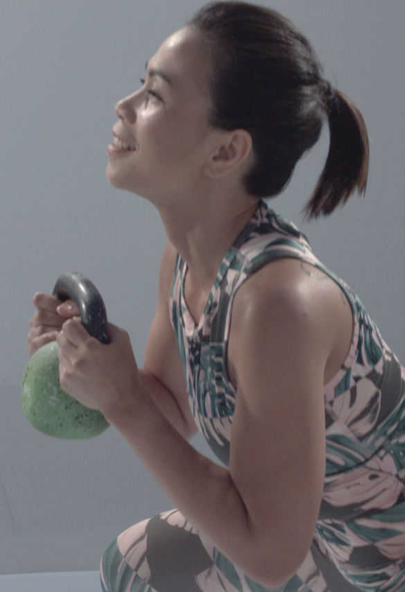
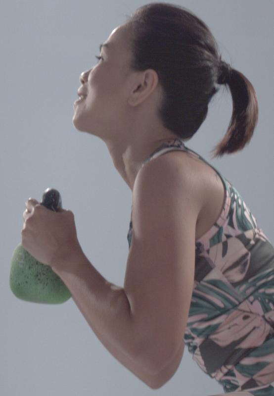
On multi-view data, conditioning on the viewing direction reduces the presence of subtle, smoke-like artifacts, which the canonical volume typically employs to model view-dependent effects without view conditioning. This is especially visible for the specularities on the face and the handle of the kettlebell. Without view-dependent effects, the reconstructed face still appears to exhibit specularities, but these are incorrectly modeled via smoke-like artifacts in the surrounding air. See Fig. S.5 and the supplemental video for results.
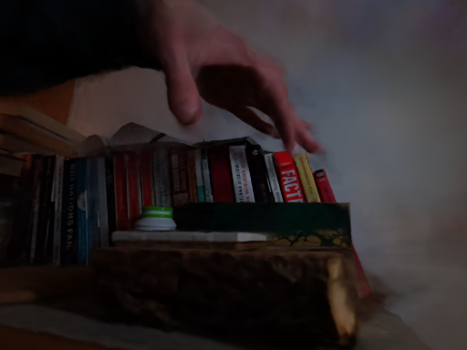
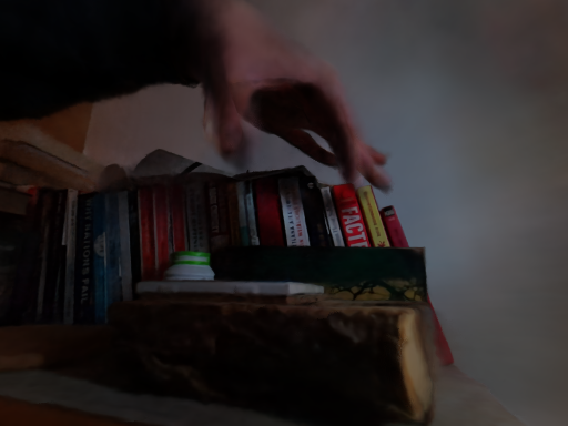
For quantitative results on monocular sequences, see Tab. S.1. However, as Fig. S.6 shows, we find our formulation to lead to artifacts in some cases. We hypothesize that the combination of both significant motion and novel views significantly different from input views is too underconstrained for view-dependent effects. For example, non-rigid NeRF might incorrectly overfit to subtle correlations between deformation and camera position at training time. However, we want to emphasize that better formulations and regularization in future work may make view-dependent effects work in these challenging scenarios.
| Ours | Ours | Ours | Naïve | Rigid | Rigid | NV | NV | |
|---|---|---|---|---|---|---|---|---|
| (appx.) | (exact) | (cond.) | (no cond.) | (mod.) | ||||
| PSNR | 24.70 | 25.07 | 22.24 | 21.88 | 14.13 | 14.10 | ||
| SSIM | 0.758 | 0.738 | 0.662 | 0.659 | 0.259 | 0.263 | ||
| LPIPS | 0.197 | 0.226 | 0.309 | 0.313 | 0.580 | 0.583 |
|
|
||
|
|
||
 |
 |
 |
 |
 |
 |
 |
| no (default) | approximate | exact |
| a) | |||
 |
 |
||
| Left Scene | Right Scene | ||
| b) | |||
| Ours | Ours (approx. view) | ||
| . | |||
| Ours (exact view) | Naïve NR-NeRF | ||
| . | |||
| Neural Volumes | Neural Volumes (modified) | ||
S.9 Simple Scene Editing
We can manipulate the learned model in further simple ways: foreground removal, temporal super-sampling, deformation exaggeration or dampening, and forced background stabilization. Having discussed only foreground removal in the main paper due to space constraints, we here present the other editing tasks.
S.9.1 Time Interpolation
We can linearly interpolate between consecutive time steps to enable temporal super-resolution since NR-NeRF optimizes a latent code for every time step . We refer to the supplemental video for results.
 |
 |
 |
 |
 |
 |
| Canonical | Dampening | Normal | Exaggeration | Exaggeration | Exaggeration |
 |
 |
 |
 |
 |
 |
| Canonical | Dampening | Dampening | Normal | Exaggeration | Exaggeration |
S.9.2 Deformation Exaggeration/Dampening
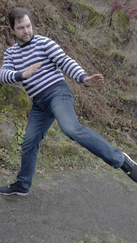
We can manipulate the deformation even further. Specifically, We can exaggerate or dampen deformations relative to the canonical model by scaling all offsets with a constant : . Fig. S.8 contains examples.
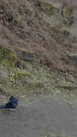
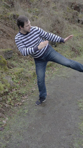
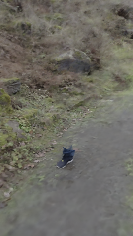


S.9.3 Forced Background Stabilization
Since we do not require any pre-computed foreground-background segmentation, NR-NeRF has to assign rigidity scores without supervision. Occasionally, this insufficiently constrains the background and leads to small motion. We can fix this in some cases by enforcing a stable background at test time: we set the regressed score to 0 if it is below some threshold . If the rigid background has sufficiently small scores assigned to it relative to the non-rigid part of the scene, this forces the background to remain static for all time steps and views. For results, we refer to the supplemental video.
S.10 Limitations
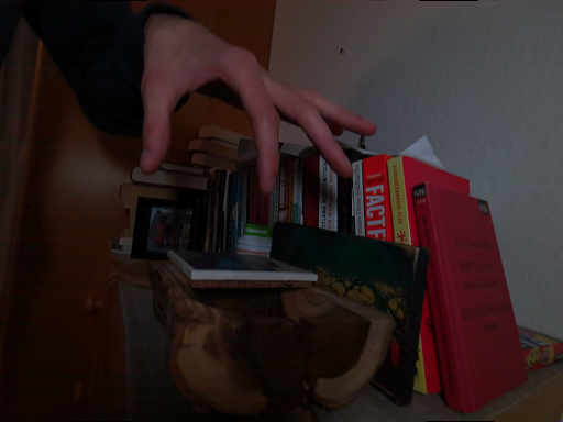
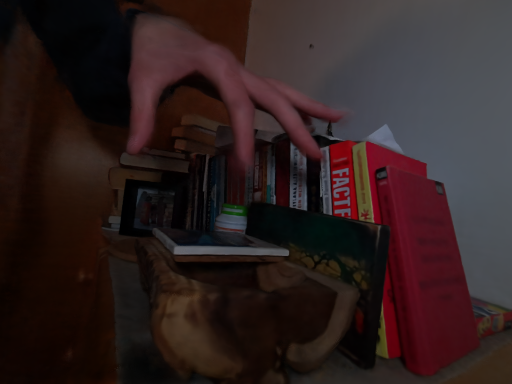
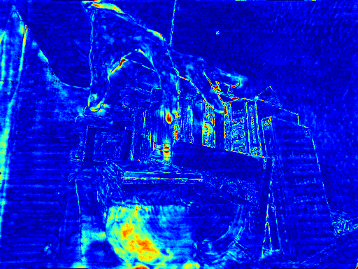
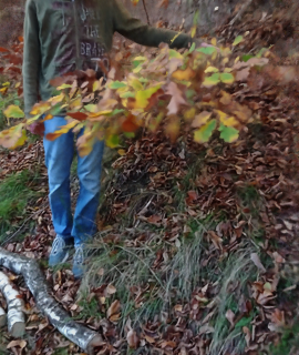
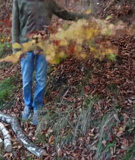
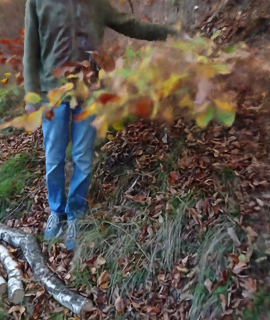
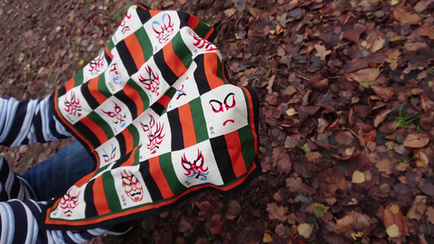
We do not account for appearance changes that are due to deformation or lighting changes. For example, temporally changing shadowing in the input images is an issue, as Fig. S.10 demonstrates.
Foreground removal can fail if a part of the foreground is entirely static (e.g., the foot in Fig. S.9).
S.11 Additional Comparisons
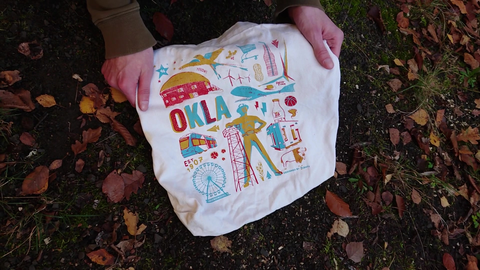
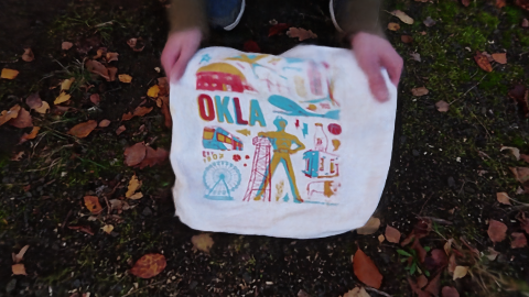
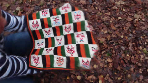
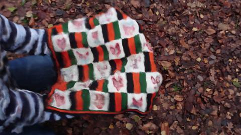
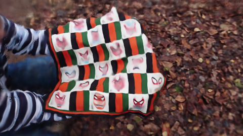
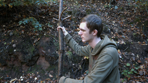
We show some preliminary qualitative comparisons to the concurrent, non-peer-reviewed work Neural Scene Flow Fields [38] in Fig. S.11.
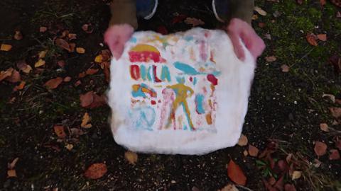
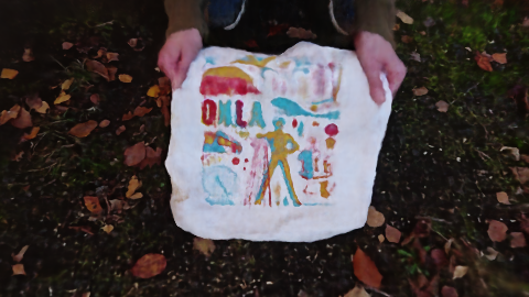
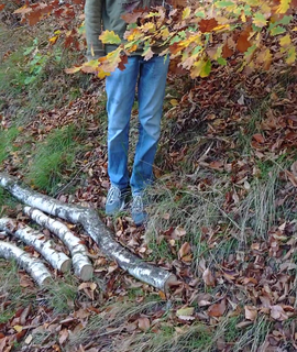
| Input | Ours | NSFF [38] | Naïve NR-NeRF | Rigid (no view dep.) | Rigid (view dep.) |
|---|---|---|---|---|---|
 |
 |
 |
 |
 |
 |
 |
 |
 |
 |
 |
 |
 |
 |
 |
 |
 |
 |
 |
 |
 |
 |
 |
 |
References
- [1] Sameer Agarwal, Yasutaka Furukawa, Noah Snavely, Ian Simon, Brian Curless, Steven M. Seitz, and Richard Szeliski. Building rome in a day. Commun. ACM, 54(10):105–112, 2011.
- [2] Guha Balakrishnan, Amy Zhao, Adrian V. Dalca, Frédo Durand, and John V. Guttag. Synthesizing images of humans in unseen poses. Computer Vision and Pattern Recognition (CVPR), 2018.
- [3] Harsh Bhatia, Gregory Norgard, Valerio Pascucci, and Peer-Timo Bremer. The helmholtz-hodge decomposition—a survey. IEEE Transactions on Visualization and Computer Graphics (TVCG), 19(8):1386–1404, 2012.
- [4] Chris Buehler, Michael Bosse, Leonard McMillan, Steven J. Gortler, and Michael F. Cohen. Unstructured lumigraph rendering. In SIGGRAPH, 2001.
- [5] Cedric Cagniart, Edmond Boyer, and Slobodan Ilic. Free-form mesh tracking: A patch-based approach. Computer Vision and Pattern Recognition (CVPR), pages 1339–1346, 2010.
- [6] Cedric Cagniart, Edmond Boyer, and Slobodan Ilic. Probabilistic deformable surface tracking from multiple videos. In European Conference on Computer Vision (ECCV), 2010.
- [7] Rodrigo L. Carceroni and Kiriakos N. Kutulakos. Multi-view scene capture by surfel sampling: From video streams to non-rigid 3d motion, shape and reflectance. International Journal of Computer Vision, 49(2):175–214, 2002.
- [8] Caroline Chan, Shiry Ginosar, Tinghui Zhou, and Alexei A Efros. Everybody dance now. In International Conference on Computer Vision (ICCV), 2019.
- [9] Alvaro Collet, Ming Chuang, Pat Sweeney, Don Gillett, Dennis Evseev, David Calabrese, Hugues Hoppe, Adam Kirk, and Steve Sullivan. High-quality streamable free-viewpoint video. ACM Transactions on Graphics (ToG), 34(4):69, 2015.
- [10] Mingsong Dou, Sameh Khamis, Yury Degtyarev, Philip Davidson, Sean Ryan Fanello, Adarsh Kowdle, Sergio Orts Escolano, Christoph Rhemann, David Kim, Jonathan Taylor, and et al. Fusion4d: Real-time performance capture of challenging scenes. ACM Trans. Graph., 35(4), 2016.
- [11] Yilun Du, Yinan Zhang, Hong-Xing Yu, Joshua B. Tenenbaum, and Jiajun Wu. Neural radiance flow for 4d view synthesis and video processing. arXiv preprint arXiv:2012.09790, 2020.
- [12] Bernhard Egger, William A. P. Smith, Ayush Tewari, Stefanie Wuhrer, Michael Zollhoefer, Thabo Beeler, Florian Bernard, Timo Bolkart, Adam Kortylewski, Sami Romdhani, Christian Theobalt, Volker Blanz, and Thomas Vetter. 3d morphable face models - past, present and future. ACM Transactions on Graphics, 39(5), Aug. 2020.
- [13] SM Ali Eslami, Danilo Jimenez Rezende, Frederic Besse, Fabio Viola, Ari S Morcos, Marta Garnelo, Avraham Ruderman, Andrei A Rusu, Ivo Danihelka, Karol Gregor, et al. Neural scene representation and rendering. Science, 360(6394):1204–1210, 2018.
- [14] John Flynn, Michael Broxton, Paul Debevec, Matthew DuVall, Graham Fyffe, Ryan Overbeck, Noah Snavely, and Richard Tucker. Deepview: View synthesis with learned gradient descent. International Conference on Computer Vision and Pattern Recognition (CVPR), 2019.
- [15] Guy Gafni, Justus Thies, Michael Zollhöfer, and Matthias Nießner. Dynamic Neural Radiance Fields for Monocular 4D Facial Avatar Reconstruction. arXiv e-prints, 2020.
- [16] Chen Gao, Yichang Shih, Wei-Sheng Lai, Chia-Kai Liang, and Jia-Bin Huang. Portrait Neural Radiance Fields from a Single Image. arXiv e-prints, 2020.
- [17] Ravi Garg, Anastasios Roussos, and Lourdes Agapito. Dense variational reconstruction of non-rigid surfaces from monocular video. Computer Vision and Pattern Recognition (CVPR), pages 1272–1279, 2013.
- [18] Vladislav Golyanik, Soshi Shimada, Kiran Varanasi, and Didier Stricker. Hdm-net: Monocular non-rigid 3d reconstruction with learned deformation model. In EuroVR, 2018.
- [19] Steven J. Gortler, Radek Grzeszczuk, Richard Szeliski, and Michael F. Cohen. The lumigraph. In SIGGRAPH, page 43–54, 1996.
- [20] Will Grathwohl, Ricky TQ Chen, Jesse Bettencourt, Ilya Sutskever, and David Duvenaud. Ffjord: Free-form continuous dynamics for scalable reversible generative models. arXiv preprint arXiv:1810.01367, 2018.
- [21] Kaiwen Guo, Peter Lincoln, Philip Davidson, Jay Busch, Xueming Yu, Matt Whalen, Geoff Harvey, Sergio Orts-Escolano, Rohit Pandey, Jason Dourgarian, and et al. The relightables: Volumetric performance capture of humans with realistic relighting. ACM Trans. Graph., 38(6), 2019.
- [22] Kaiwen Guo, Feng Xu, Tao Yu, Xiaoyang Liu, Qionghai Dai, and Yebin Liu. Real-time geometry, albedo, and motion reconstruction using a single rgb-d camera. ACM Trans. Graph., 36(4), 2017.
- [23] Marc Habermann, Weipeng Xu, Michael Zollhöfer, Gerard Pons-Moll, and Christian Theobalt. Livecap: Real-time human performance capture from monocular video. ACM Trans. Graph., 38(2):14:1–14:17, Mar. 2019.
- [24] Peter Hedman, Julien Philip, True Price, Jan-Michael Frahm, George Drettakis, and Gabriel Brostow. Deep blending for free-viewpoint image-based rendering. ACM Trans. Graph., 37(6):257:1–257:15, Dec. 2018.
- [25] Zeng Huang, Tianye Li, Weikai Chen, Yajie Zhao, Jun Xing, Chloe Legendre, Linjie Luo, Chongyang Ma, and Hao Li. Deep volumetric video from very sparse multi-view performance capture. In European Conference on Computer Vision (ECCV), pages 351–369, 2018.
- [26] Michael F Hutchinson. A stochastic estimator of the trace of the influence matrix for laplacian smoothing splines. Communications in Statistics-Simulation and Computation, 18(3):1059–1076, 1989.
- [27] Takeo Igarashi, Tomer Moscovich, and John F Hughes. As-rigid-as-possible shape manipulation. ACM transactions on Graphics (TOG), 24(3):1134–1141, 2005.
- [28] Matthias Innmann, Michael Zollhöfer, Matthias Nießner, Christian Theobald, and Marc Stamminger. Volumedeform: Real-time volumetric non-rigid reconstruction. In European Conference on Computer Vision (ECCV), 2016.
- [29] Hyeongwoo Kim, Mohamed Elgharib, Hans-Peter Zollöfer, Michael Seidel, Thabo Beeler, Christian Richardt, and Christian Theobalt. Neural style-preserving visual dubbing. ACM Transactions on Graphics (TOG), 38(6):178:1–13, 2019.
- [30] Hyeongwoo Kim, Pablo Garrido, Ayush Tewari, Weipeng Xu, Justus Thies, Matthias Nießner, Patrick Pérez, Christian Richardt, Michael Zollöfer, and Christian Theobalt. Deep video portraits. ACM Transactions on Graphics (TOG), 37, 2018.
- [31] Diederik P Kingma and Jimmy Ba. Adam: A method for stochastic optimization. arXiv preprint arXiv:1412.6980, 2014.
- [32] Muhammed Kocabas, Nikos Athanasiou, and Michael J. Black. VIBE: Video inference for human body pose and shape estimation. In Proceedings IEEE Conf. on Computer Vision and Pattern Recognition (CVPR), pages 5252–5262. IEEE, June 2020.
- [33] Suryansh Kumar, Anoop Cherian, Yuchao Dai, and Hongdong Li. Scalable dense non-rigid structure-from-motion: A grassmannian perspective. In Computer Vision and Pattern Recognition (CVPR), 2018.
- [34] Kiriakos N. Kutulakos and Steven M. Seitz. A theory of shape by space carving. International Journal of Computer Vision (IJCV), 38:199–218, 2000.
- [35] Marc Levoy and Pat Hanrahan. Light field rendering. In SIGGRAPH, page 31–42, 1996.
- [36] Guannan Li, Chenglei Wu, Carsten Stoll, Yebin Liu, Kiran Varanasi, Qionghai Dai, and Christian Theobalt. Capturing relightable human performances under general uncontrolled illumination. Comput. Graph. Forum, 32(2):275–284, 2013.
- [37] Tianye Li, Mira Slavcheva, Michael Zollhoefer, Simon Green, Christoph Lassner, Changil Kim, Tanner Schmidt, Steven Lovegrove, Michael Goesele, and Zhaoyang Lv. Neural 3d video synthesis, 2021.
- [38] Zhengqi Li, Simon Niklaus, Noah Snavely, and Oliver Wang. Neural Scene Flow Fields for Space-Time View Synthesis of Dynamic Scenes. arxiv, 2020.
- [39] Lingjie Liu, Jiatao Gu, Kyaw Zaw Lin, Tat-Seng Chua, and Christian Theobalt. Neural sparse voxel fields. Advances in Neural Information Processing Systems, 33, 2020.
- [40] Yebin Liu, Qionghai Dai, and Wenli Xu. A point-cloud-based multiview stereo algorithm for free-viewpoint video. IEEE Transactions on Visualization and Computer Graphics (TVCG), 16(3):407–418, 2010.
- [41] Stephen Lombardi, Tomas Simon, Jason Saragih, Gabriel Schwartz, Andreas Lehrmann, and Yaser Sheikh. Neural volumes: Learning dynamic renderable volumes from images. ACM Trans. Graph. (SIGGRAPH), 38(4), 2019.
- [42] Liqian Ma, Qianru Sun, Stamatios Georgoulis, Luc Van Gool, Bernt Schiele, and Mario Fritz. Disentangled person image generation. Computer Vision and Pattern Recognition (CVPR), 2018.
- [43] Ricardo Martin Brualla, Peter Lincoln, Adarsh Kowdle, Christoph Rhemann, Dan Goldman, Cem Keskin, Steve Seitz, Shahram Izadi, Sean Fanello, Rohit Pandey, Shuoran Yang, Pavel Pidlypenskyi, Jonathan Taylor, Julien Valentin, Sameh Khamis, Philip Davidson, and Anastasia Tkach. Lookingood: Enhancing performance capture with real-time neural re-rendering. volume 37, 2018.
- [44] Takashi Matsuyama, Xiaojun Wu, Takeshi Takai, and Toshikazu Wada. Real-time dynamic 3-d object shape reconstruction and high-fidelity texture mapping for 3-d video. IEEE Transactions on Circuits and Systems for Video Technology, 14(3):357–369, 2004.
- [45] Moustafa Meshry, Dan B. Goldman, Sameh Khamis, Hugues Hoppe, Rohit Pandey, Noah Snavely, and Ricardo Martin-Brualla. Neural rerendering in the wild. In Computer Vision and Pattern Recognition (CVPR), 2019.
- [46] Ben Mildenhall, Pratul P. Srinivasan, Matthew Tancik, Jonathan T. Barron, Ravi Ramamoorthi, and Ren Ng. Nerf: Representing scenes as neural radiance fields for view synthesis. In ECCV, 2020.
- [47] Ben Mildenhall, Pratul P. Srinivasan, Matthew Tancik, Jonathan T. Barron, Ravi Ramamoorthi, and Ren Ng. Nerf: Representing scenes as neural radiance fields for view synthesis. In European Conference on Computer Vision (ECCV), 2020.
- [48] Graham Miller, Adrian Hilton, and Jonathan Starck. Interactive free-viewpoint video. In IEEE European Conf. on Visual Media Production, pages 50–59, 2005.
- [49] Koki Nagano, Graham Fyffe, Oleg Alexander, Jernej Barbiç, Hao Li, Abhijeet Ghosh, and Paul Debevec. Skin microstructure deformation with displacement map convolution. ACM Trans. Graph., 34(4), 2015.
- [50] Natalia Neverova, Riza Alp Güler, and Iasonas Kokkinos. Dense pose transfer. ECCV, 2018.
- [51] Richard A. Newcombe, Dieter Fox, and Steven M. Seitz. Dynamicfusion: Reconstruction and tracking of non-rigid scenes in real-time. In Computer Vision and Pattern Recognition (CVPR), 2015.
- [52] Richard A. Newcombe, Shahram Izadi, Otmar Hilliges, David Kim, Andrew J. Davison, Pushmeet Kohli, Jamie Shotton, Steve Hodges, and Andrew Fitzgibbon. Kinectfusion: Real-time dense surface mapping and tracking. In International Symposium on Mixed and Augmented Reality (ISMAR), 2011.
- [53] Dat Tien Ngo, Sanghyuk Park, Anne Jorstad, Alberto Crivellaro, Chang D. Yoo, and Pascal Fua. Dense image registration and deformable surface reconstruction in presence of occlusions and minimal texture. In International Conference on Computer Vision (ICCV), 2015.
- [54] Thu H Nguyen-Phuoc, Chuan Li, Stephen Balaban, and Yongliang Yang. Rendernet: A deep convolutional network for differentiable rendering from 3d shapes. In Advances in Neural Information Processing Systems (NIPS), 2018.
- [55] Sergio Orts-Escolano, Christoph Rhemann, Sean Fanello, Wayne Chang, Adarsh Kowdle, Yury Degtyarev, David Kim, Philip L. Davidson, Sameh Khamis, Mingsong Dou, and et al. Holoportation: Virtual 3d teleportation in real-time. In Annual Symposium on User Interface Software and Technology, page 741–754, 2016.
- [56] Martin R. Oswald, Jan Stühmer, and Daniel Cremers. Generalized connectivity constraints for spatio-temporal 3d reconstruction. In European Conference on Computer Vision (ECCV), 2014.
- [57] Jeong Joon Park, Peter Florence, Julian Straub, Richard Newcombe, and Steven Lovegrove. Deepsdf: Learning continuous signed distance functions for shape representation. International Conference on Computer Vision and Pattern Recognition (CVPR), 2019.
- [58] Keunhong Park, Utkarsh Sinha, Jonathan T. Barron, Sofien Bouaziz, Dan B Goldman, Steven M. Seitz, and Ricardo Martin-Brualla. Deformable neural radiance fields. arXiv preprint arXiv:2011.12948, 2020.
- [59] Adam Paszke, Sam Gross, Francisco Massa, Adam Lerer, James Bradbury, Gregory Chanan, Trevor Killeen, Zeming Lin, Natalia Gimelshein, Luca Antiga, Alban Desmaison, Andreas Kopf, Edward Yang, Zachary DeVito, Martin Raison, Alykhan Tejani, Sasank Chilamkurthy, Benoit Steiner, Lu Fang, Junjie Bai, and Soumith Chintala. Pytorch: An imperative style, high-performance deep learning library. In H. Wallach, H. Larochelle, A. Beygelzimer, F. d'Alché-Buc, E. Fox, and R. Garnett, editors, Advances in Neural Information Processing Systems 32, pages 8024–8035. Curran Associates, Inc., 2019.
- [60] Sida Peng, Yuanqing Zhang, Yinghao Xu, Qianqian Wang, Qing Shuai, Hujun Bao, and Xiaowei Zhou. Neural body: Implicit neural representations with structured latent codes for novel view synthesis of dynamic humans. arXiv e-prints, 2020.
- [61] Mathieu Perriollat, Richard Hartley, and Adrien Bartoli. Monocular template-based reconstruction of inextensible surfaces. Int. J. Comput. Vision (IJCV), 95(2):124–137, 2011.
- [62] Hanspeter Pfister, Matthias Zwicker, Jeroen van Baar, and Markus Gross. Surfels: Surface elements as rendering primitives. In Proceedings of the 27th Annual Conference on Computer Graphics and Interactive Techniques, SIGGRAPH ’00, page 335–342, USA, 2000. ACM Press/Addison-Wesley Publishing Co.
- [63] Albert Pumarola, Enric Corona, Gerard Pons-Moll, and Francesc Moreno-Noguer. D-NeRF: Neural Radiance Fields for Dynamic Scenes. arxiv, 2020.
- [64] Amit Raj, Michael Zollhoefer, Tomas Simon, Jason Saragih, Shunsuke Saito, James Hays, and Stephen Lombardi. Pva: Pixel-aligned volumetric avatars, 2021.
- [65] Gernot Riegler and Vladlen Koltun. Free view synthesis. In European Conference on Computer Vision (ECCV), 2020.
- [66] Kripasindhu Sarkar, Dushyant Mehta, Weipeng Xu, Vladislav Golyanik, and Christian Theobalt. Neural re-rendering of humans from a single image. In European Conference on Computer Vision (ECCV), 2020.
- [67] Johannes L Schonberger and Jan-Michael Frahm. Structure-from-motion revisited. In Proceedings of the IEEE Conference on Computer Vision and Pattern Recognition, pages 4104–4113, 2016.
- [68] Johannes Lutz Schönberger and Jan-Michael Frahm. Structure-from-motion revisited. In Computer Vision and Pattern Recognition (CVPR), 2016.
- [69] Johannes Lutz Schönberger, Enliang Zheng, Marc Pollefeys, and Jan-Michael Frahm. Pixelwise view selection for unstructured multi-view stereo. In European Conference on Computer Vision (ECCV), 2016.
- [70] Jonathan Shade, Steven Gortler, Li-wei He, and Richard Szeliski. Layered depth images. In Proceedings of the 25th Annual Conference on Computer Graphics and Interactive Techniques, SIGGRAPH ’98, page 231–242, New York, NY, USA, 1998. Association for Computing Machinery.
- [71] Aliaksandra Shysheya, Egor Zakharov, Kara-Ali Aliev, Renat Bashirov, Egor Burkov, Karim Iskakov, Aleksei Ivakhnenko, Yury Malkov, Igor Pasechnik, Dmitry Ulyanov, Alexander Vakhitov, and Victor Lempitsky. Textured neural avatars. In Computer Vision and Pattern Recognition (CVPR), 2019.
- [72] Vikramjit Sidhu, Edgar Tretschk, Vladislav Golyanik, Antonio Agudo, and Christian Theobalt. Neural dense non-rigid structure from motion with latent space constraints. In European Conference on Computer Vision (ECCV), 2020.
- [73] Vincent Sitzmann, Justus Thies, Felix Heide, Matthias Niessner, Gordon Wetzstein, and Michael Zollhofer. Deepvoxels: Learning persistent 3d feature embeddings. In Computer Vision and Pattern Recognition (CVPR), 2019.
- [74] Vincent Sitzmann, Michael Zollhöfer, and Gordon Wetzstein. Scene representation networks: Continuous 3d-structure-aware neural scene representations. In Advances in Neural Information Processing Systems, 2019.
- [75] Miroslava Slavcheva, Maximilian Baust, Daniel Cremers, and Slobodan Ilic. Killingfusion: Non-rigid 3d reconstruction without correspondences. In Computer Vision and Pattern Recognition (CVPR), 2017.
- [76] Aljoscha Smolic, Karsten Mueller, Philipp Merkle, Christoph Fehn, Peter Kauff, Peter Eisert, and Thomas Wiegand. 3d video and free viewpoint video-technologies, applications and mpeg standards. In IEEE International Conference on Multimedia and Expo, pages 2161–2164. IEEE, 2006.
- [77] Olga Sorkine and Marc Alexa. As-rigid-as-possible surface modeling. In Symposium on Geometry Processing, volume 4, pages 109–116, 2007.
- [78] Jonathan Starck, Gregor Miller, and Adrian Hilton. Volumetric stereo with silhouette and feature constraints. In British Machine Vision Conference (BMVC), 2006.
- [79] Shih-Yang Su, Frank Yu, Michael Zollhoefer, and Helge Rhodin. A-nerf: Surface-free human 3d pose refinement via neural rendering, 2021.
- [80] Shufeng Tan and Michael L. Mayrovouniotis. Reducing data dimensionality through optimizing neural network inputs. AIChE Journal, 41(6):1471–1480, 1995.
- [81] Yu Tao, Zerong Zheng, Kaiwen Guo, Jianhui Zhao, Dai Quionhai, Hao Li, Gerard Pons-Moll, and Yebin Liu. Doublefusion: Real-time capture of human performance with inner body shape from a depth sensor. In Computer Vision and Pattern Recognition (CVPR), 2018.
- [82] Ayush Tewari, Ohad Fried, Justus Thies, Vincent Sitzmann, Stephen Lombardi, Kalyan Sunkavalli, Ricardo Martin-Brualla, Tomas Simon, Jason Saragih, Matthias Nießner, Rohit Pandey, Sean Fanello, Gordon Wetzstein, Jun-Yan Zhu, Christian Theobalt, Maneesh Agrawala, Eli Shechtman, Dan B Goldman, and Michael Zollhöfer. State of the Art on Neural Rendering. Computer Graphics Forum (EG STAR 2020), 2020.
- [83] Christian Theobalt, Naveed Ahmed, Hendrik Lensch, Marcus Magnor, and Hans-Peter Seidel. Seeing people in different light-joint shape, motion, and reflectance capture. IEEE Transactions on Visualization and Computer Graphics (TVCG), 13(4):663–674, 2007.
- [84] Justus Thies, Michael Zollhöfer, and Matthias Nießner. Deferred neural rendering: image synthesis using neural textures. ACM Transactions on Graphics, 38, 2019.
- [85] Edgar Tretschk, Ayush Tewari, Michael Zollhöfer, Vladislav Golyanik, and Christian Theobalt. DEMEA: Deep mesh autoencoders for non-rigidly deforming objects. In European Conference on Computer Vision (ECCV), 2020.
- [86] Tony Tung, Shohei Nobuhara, and Takashi Matsuyama. Complete multi-view reconstruction of dynamic scenes from probabilistic fusion of narrow and wide baseline stereo. pages 1709–1716, 2009.
- [87] Ziyan Wang, Timur Bagautdinov, Stephen Lombardi, Tomas Simon, Jason Saragih, Jessica Hodgins, and Michael Zollhöfer. Learning Compositional Radiance Fields of Dynamic Human Heads. arXiv e-prints, 2020.
- [88] Michael Waschbüsch, Stephan Würmlin, Daniel Cotting, Filip Sadlo, and Markus Gross. Scalable 3d video of dynamic scenes. The Visual Computer, 21(8):629–638, 2005.
- [89] Chung-Yi Weng, Brian Curless, and Ira Kemelmacher-Shlizerman. Vid2Actor: Free-viewpoint Animatable Person Synthesis from Video in the Wild. arXiv e-prints, 2020.
- [90] Wenqi Xian, Jia-Bin Huang, Johannes Kopf, and Changil Kim. Space-time neural irradiance fields for free-viewpoint video. arXiv preprint, 2020.
- [91] Donglai Xiang, Hanbyul Joo, and Yaser Sheikh. Monocular total capture: Posing face, body, and hands in the wild. In Proceedings of the IEEE Conference on Computer Vision and Pattern Recognition, pages 10965–10974, 2019.
- [92] Weipeng Xu, Avishek Chatterjee, Michael Zollhöfer, Helge Rhodin, Dushyant Mehta, Hans-Peter Seidel, and Christian Theobalt. Monoperfcap: Human performance capture from monocular video. ACM Trans. Graph., 37(2):27:1–27:15, 2018.
- [93] Lin Yen-Chen. Nerf-pytorch. https://github.com/yenchenlin/nerf-pytorch/, 2020.
- [94] Jae Shin Yoon, Kihwan Kim, Orazio Gallo, Hyun Soo Park, and Jan Kautz. Novel view synthesis of dynamic scenes with globally coherent depths from a monocular camera. 2020.
- [95] Rui Yu, Chris Russell, Neill D. F. Campbell, and Lourdes Agapito. Direct, dense, and deformable: Template-based non-rigid 3d reconstruction from rgb video. In International Conference on Computer Vision (ICCV), 2015.
- [96] Tao Yu, Kaiwen Guo, Feng Xu, Yuan Dong, Zhaoqi Su, Jianhui Zhao, Jianguo Li, Qionghai Dai, and Yebin Liu. Bodyfusion: Real-time capture of human motion and surface geometry using a single depth camera. In International Conference on Computer Vision (ICCV), pages 910–919, 2017.
- [97] Tao Yu, Zerong Zheng, Yuan Zhong, Jianhui Zhao, Qionghai Dai, Gerard Pons-Moll, and Yebin Liu. Simulcap : Single-view human performance capture with cloth simulation. In Conference on Computer Vision and Pattern Recognition(CVPR), 2019.
- [98] Kai Zhang, Gernot Riegler, Noah Snavely, and Vladlen Koltun. Nerf++: Analyzing and improving neural radiance fields. arXiv preprint arXiv:2010.07492, 2020.
- [99] Li Zhang, Brian Curless, and Steven M. Seitz. Spacetime stereo: shape recovery for dynamic scenes. In Computer Vision and Pattern Recognition (CVPR), 2003.
- [100] Richard Zhang, Phillip Isola, Alexei A Efros, Eli Shechtman, and Oliver Wang. The unreasonable effectiveness of deep features as a perceptual metric. In Computer Vision and Pattern Recognition (CVPR), 2018.
- [101] Zhou Wang, Alan C. Bovik, Hamid R. Sheikh, and Eero P. Simoncelli. Image quality assessment: from error visibility to structural similarity. IEEE Transactions on Image Processing, 13(4):600–612, 2004.
- [102] Hao Zhu, Hao Su, Peng Wang, Xun Cao, and Ruigang Yang. View extrapolation of human body from a single image. In Computer Vision and Pattern Recognition (CVPR), 2018.
- [103] Michael Zollhöfer, Matthias Nießner, Shahram Izadi, Christoph Rhemann, Christopher Zach, Matthew Fisher, Chenglei Wu, Andrew Fitzgibbon, Charles Loop, Christian Theobalt, and Marc Stamminger. Real-time non-rigid reconstruction using an rgb-d camera. ACM Transactions on Graphics (TOG), 2014.
- [104] Michael Zollhöfer, Patrick Stotko, Andreas Görlitz, Christian Theobalt, Matthias Nießner, Reinhard Klein, and Andreas Kolb. State of the art on 3d reconstruction with rgb-d cameras. In Computer graphics forum, volume 37, pages 625–652. Wiley Online Library, 2018.