A Phaseless Auxiliary-Field Quantum Monte Carlo Perspective on the Uniform Electron Gas at Finite Temperatures: Issues, Observations, and Benchmark Study

Abstract

We investigate the viability of the phaseless finite temperature auxiliary field quantum Monte Carlo (ph-FT-AFQMC) method for ab initio systems using the uniform electron gas as a model. Through comparisons with exact results and finite temperature coupled cluster theory, we find that ph-FT-AFQMC is sufficiently accurate at high to intermediate electronic densities. We show both analytically and numerically that the phaseless constraint at finite temperature is fundamentally different from its zero temperature counterpart (i.e., ph-ZT-AFQMC) and generally one should not expect ph-FT-AFQMC to agree with ph-ZT-AFQMC in the low temperature limit. With an efficient implementation, we are able to compare exchange-correlation energies to existing results in the thermodynamic limit and find that existing parameterizations are highly accurate. In particular, we found that ph-FT-AFQMC exchange-correlation energies are in a better agreement with a known parametrization than is restricted path-integral Monte Carlo in the regime of $\Theta\leq 0.5$ and $r_{s}\leq 2$, which highlights the strength of ph-FT-AFQMC.

I Introduction

Temperature-dependent properties of interacting fermions are fundamentally important in both experiments and theory. Typical phenomena at finite temperature include the BCS-BEC crossover in the attractive 2D Fermi model,(Petrov et al., 2003) the competition between stripe and superconducting orders in the two-dimensional Hubbard model,(Qin et al., 2020) and plasmonic catalysis.(Mukherjee et al., 2013) Furthermore, there is a growing interest in warm-dense matter,(Graziani, 2014) an extreme state of matter found in planetary interiors(Fortney et al., 2009) that can be created with high intensity lasers.(Koenig et al., 2005; Ernstorfer et al., 2009) Understanding such phenomena at the theoretical level is challenging due to the delicate interplay between electron-electron, electron-ion, quantum mechanical and thermal effects all of which can be equally important and often cannot be treated perturbatively. Thus, accurate computational approaches are required that are capable of capturing these effects.

Density functional theory (DFT), as the workhorse of zero temperature electronic structure theory, is an ideal candidate: it is relatively cheap and accurate, it can be coupled with molecular dynamics to include ionic effects and it can be rigorously formulated to incorporate thermal electronic effects.(Mermin, 1965) Indeed, DFT has proven itself effective in simulating warm dense matter.(Driver et al., 2015; Zhang et al., 2016, 2017; Driver et al., 2017) However, questions remain regarding the accuracy of using approximations made in thermal DFT, including the accuracy of the use of zero temperature exchange correlation functionals.(Karasiev et al., 2016, 2019; Ramakrishna et al., 2020; Mihaylov et al., 2020) Complementary approaches are therefore desired that can benchmark or supplement DFT results when necessary.

Quantum Monte Carlo (QMC) methods are a promising class of such computational methods. They are in principle exact in a finite supercell and can explicitly include many-body and thermal effects in an unbiased way. Of the many flavors of QMC, real space path integral Monte Carlo (PIMC) is perhaps the best known and well established.(Ceperley, 1995) PIMC, as a real space approach, works in the complete basis set limit which is a considerable benefit at very high electronic temperatures. However, like all fermionic QMC methods it suffers from the sign problem which can only be overcome using the uncontrolled restricted path approximation,(Ceperley, 1991) which leads to the restricted PIMC (RPIMC) approach. This approach is similar in spirit to the fixed-node approximation in diffusion Monte Carlo (DMC),(Foulkes et al., 2001) but now a constraint is enforced using a trial thermal density matrix. The quality of this constraint is a priori unknown, however, results with free fermion nodes in the uniform electron gas (UEG) suggest that it is unreliable at high densities and at lower temperatures.(Brown et al., 2013a; Schoof et al., 2015a; Malone et al., 2016) We note there have been promising developments in extending the scope of PIMC to higher densities and lower temperatures through algorithmic developments(DuBois et al., ) including the development of new algorithms such as the in principle exact real space permutation blocking PIMC(Dornheim et al., 2015) (PB-PIMC) and second quantized configuration PIMC(Schoof et al., 2011) (CPIMC). In particular, PB-PIMC and CPIMC have been used as complementary approaches to simulate the warm dense UEG above half the Fermi temperature, with the fermion sign problem preventing simulations below this. We note that restricted CPIMC may be a promising route to access lower temperature given its results on small UEG supercells and the 33-electron supercell spin-polarized case.Yilmaz et al. (2020) Other interesting QMC approaches are the quantum chemistry inspired methods like density matrix quantum Monte Carlo(Blunt et al., 2014; Malone et al., 2015; Petras et al., 2020) (DMQMC) and krylov-projected full configuration interaction quantum Monte Carlo.(Blunt et al., 2015) Like CPIMC these approaches work in a second quantized space and work well at high densities, however they often struggle to reach the complete basis set limit. All of these methods offer unbiased exact thermal expectation values in principle, however, they all ultimately scale exponentially with the number of electrons in general. See Ref.31 for a review of the parameter regimes accessible to these new QMC methods.

Recently there has also been considerable interest in developing finite temperature deterministic quantum chemistry methods that work in a finite basis set. These methods include second order perturbation theory,(He et al., 2014; Santra and Schirmer, 2017; Hirata and Jha, 2020; Jha and Hirata, 2020) coupled cluster theory(Hermes and Hirata, 2015; White and Chan, 2018, 2020) and thermofield theory.(Harsha et al., 2019) These are promising and offer a systematic approach to including electronic temperature effects, but they often struggle to reach the continuum limit (also known as the complete basis set (CBS) limit) due to the steep computational scaling with respect to the number of basis functions, $M$. For example, FT-CCSD scales like $\mathcal{O}(M^{6})$, which becomes prohibitively expensive to converge results to the CBS limit.(White and Chan, 2018, 2020)

Finite temperature auxiliary-Field QMC(Blankenbecler et al., 1981; Scalapino and Sugar, 1981) (FT-AFQMC) is another promising QMC method. It works in the second quantized space and thereby suffers from the basis set incompleteness errors common to DMQMC and CPIMC. However, unlike DMQMC and CPIMC, it can be made to scale polynomially with system size at the cost of introducing an uncontrolled bias called the phaseless approximation.(Zhang and Krakauer, 2003; Zhang, 1999) Moreover, zero temperature phaseless AFQMC (ph-ZT-AFQMC) has proven itself as one of the most accurate and scalable post Hartree–Fock methods.(LeBlanc et al., 2015; Motta et al., 2017; Williams et al., 2020; Lee et al., 2020a, b) In addition, the bias introduced by the phaseless approximation is typically much smaller than the fixed node-error in DMC(Malone et al., 2020a) which in principle should serve as an rough upper bound to the bias in RPIMC. Thus, it is important to assess the quality of ph-FT-AFQMC for realistic systems as to date the applications have largely focussed on model systems(He et al., 2019a; Rubenstein et al., 2012) or have not enforced the constraint(Liu et al., 2018, 2020; Shen et al., 2020) which is not a practical approach as the system size increases. Compared to FT-CCSD, ph-FT-AFQMC maintains favorable cubic scaling $\mathcal{O}(M^{3})$ for each statistical sample,Lee and Reichman (2020); Malone et al. (2019) which makes it better-suited for large-scale warm dense matter simulations.

In this paper, we investigate the viability of ph-FT-AFQMC both in terms of its accuracy and in its ability to reach the complete basis set limit. We stress good performance for both of these metrics is critical if the method is to be practically useful for finite-temperature ab-initio systems. To address these problems we use the uniform electron gas (UEG) model as a testbed for ph-FT-AFQMC. To the best of our knowledge, our work is the first to apply ph-FT-AFQMC at finite temperature beyond lattice models with short-range interactions. The main goal of our work is to assess the accuracy of ph-FT-AFQMC when applied to the UEG model.

Apart from being a foundational model in condensed matter physics,(Giuliani and Vignale, 2005; Ceperley and Alder, 1980; Perdew and Zunger, 1981; Perdew et al., 1996) the UEG offers a number of useful features from a computational point of view. First, the model can be tuned from weak to strong correlation as a function of the density parameter, $r_{s}$. Given that our previous work(Lee et al., 2019) has shown that ph-ZT-AFQMC is highly accurate for $r_{s}\leq 3-4$ at zero temperature and we have an idea of the magnitude of errors we might expect. Second, basis set convergence can be easily investigated in a planewave basis set by increasing the energy cutoff. Finally, the UEG at warm dense matter conditions has been the subject of intense study over the past decade.(Dornheim et al., 2018a) In fact many of the recent developments(Dornheim et al., 2018a) in finite temperature fermionic QMC methods was spurred on by a discrepancy between RPIMC and CPIMC(Brown et al., 2013b; Schoof et al., 2015b) results for the warm dense UEG that have been incorporated into finite temperature exchange correlation functionals.(Brown et al., 2013c; Karasiev et al., 2014; Groth et al., 2017a) Because of this effort there is a considerable amount of essentially exact data for energetic,(Groth et al., 2016; Dornheim et al., 2016a) static(Dornheim et al., 2017b, c; Groth et al., 2017b) and dynamic properties(Dornheim et al., 2018b; Groth et al., 2019a) of the model at a wide range of densities and temperatures. Nonetheless, despite this immense effort, there is a gap in accurate data below roughly half the Fermi temperature below which no method could reach due to the Fermionic sign problem.(Dornheim et al., 2016b) In this paper we use ph-FT-AFQMC to partially fill this gap.

This paper is organized as follows. In the first section we outline the ph-FT-AFQMC method, paying careful attention to how to implement it efficiently in a numerically stable fashion. Next, we carefully benchmark the method at various temperatures against exact results in small basis sets and investigate the low temperature limit in comparison to the ph-ZT-AFQMC results. We also compare the ph-FT-AFQMC results to FT-CCSD and PIMC where possible. Lastly, we compare our results against other QMC methods and available excahnge-correlation parametrization in the thermodynamic limit and finish by outlining our perspective for the future of the method.

II Theory

We briefly summarize the phaseless approximation of AFQMC within the finite temperature formalism (i.e., ph-FT-AFQMC).

II.1 Finite-Temperature AFQMC in the Grand Canonical Ensemble

II.1.1 General formalisms

The finite temperature AFQMC algorithm aims to compute thermal expectation values based on the grand canonical partition function

$$Z=\operatorname{tr}(e^{-\beta(\hat{H}-\mu\hat{N})})$$ (1)

where $\hat{N}$ is a total number operator, $\mu$ is a chemical potential, and the Hamiltonian involves one-body ($\hat{H}_{1}$) and two-body ($\hat{H}_{2}$) terms,

$$\hat{H}=\hat{H}_{1}+\hat{H}_{2}$$ (2)

The direct (deterministic) evaluation of trace in Eq. 1 scales exponentially since there are exponentially many states to consider. It is then natural to consider QMC algorithms to sample an instance of the terms in $Z$.

A particular flavor of QMC that we focus on here is AFQMC where the two-body propagator is expressed by the Hubbard-Stratonovich transformation,(Hubbard, 1959)

$$e^{-\Delta\tau\hat{H}_{2}}=\int d\mathbf{x}p(\mathbf{x})e^{-\sqrt{\Delta\tau}\mathbf{x}\cdot\hat{\mathbf{v}}}$$ (3)

where $\hat{\mathbf{v}}$ is related to the two-body Hamiltonian as a sum of squared operators,

$$\hat{H}_{2}=-\frac{1}{2}\sum_{\alpha}^{N_{\alpha}}\hat{v}_{\alpha}^{2},$$ (4)

$\mathbf{x}$ is a vector of $N_{\alpha}$ auxiliary fields which are samples from the standard normal distribution, $p(\mathbf{x})$. With the symmetric Trotter decomposition, the total propagator reads

$$\exp(-\Delta\tau\hat{H})\>=\int d\mathbf{x}p(\mathbf{x})\hat{B}(\Delta\tau,\mathbf{x},\mu)$$ (5)

where $\hat{B}$ is defined as

$$\hat{B}(\Delta\tau,\mathbf{x},\mu)=e^{-\frac{\Delta\tau}{2}(\hat{H}_{1}-\mu\hat{N})}e^{-\sqrt{\Delta\tau}\mathbf{x}\cdot\hat{\mathbf{v}}}e^{-\frac{\Delta\tau}{2}(\hat{H}_{1}-\mu\hat{N})}.$$ (6)

For a given number of imaginary time slices $n$, we sample the auxiliary fields via MC,

$$Z=\sum_{\{\mathbf{x}_{1},\mathbf{x}_{2},\cdot\cdot\cdot\mathbf{x}_{n}\}} p(\mathbf{x}_{1},\mathbf{x}_{2},\cdot\cdot\cdot\mathbf{x}_{n})$$

$$\times\operatorname{tr}\left({\prod_{i=1}^{n}\hat{B}(\Delta\tau,\mathbf{x}_{i},\mu)}\right)$$ (7)

where $p(\mathbf{x}_{1},\mathbf{x}_{2},\cdot\cdot\cdot\mathbf{x}_{n})$ is the probability of sampling a specific path designated by auxiliary fields, $\mathbf{x}_{1},\mathbf{x}_{2},\cdot\cdot\cdot\mathbf{x}_{n}$, and the time step, $\Delta\tau=\beta/n$, is determined by the temperature and the number of imaginary time slices. The evaluation of the trace in Eq. 7 is still difficult because it needs to consider all possible states in the Hilbert space despite the fact that every operator inside the trace is a one-body operator. One can show analytically that the trace can be written in terms of a determinant in the grand canonical ensemble,(Blankenbecler et al., 1981; Hirsch, 1985; Dos Santos, 2003)

$$Z=\sum_{\{\mathbf{x}_{1},\mathbf{x}_{2},\cdot\cdot\cdot\mathbf{x}_{n}\}} p(\mathbf{x}_{1},\mathbf{x}_{2},\cdot\cdot\cdot\mathbf{x}_{n})$$

$$\times\det\left({\mathbf{I}+\prod_{i=1}^{n}\mathbf{B}(\Delta\tau,\mathbf{x}_{i},\mu)}\right)$$ (8)

where $\mathbf{B}$ is a matrix representation of $\hat{B}$ in the single-particle basis. For a later use, we define the product of $\mathbf{B}$ as

$$\mathbf{A}(n\Delta\tau,\{\mathbf{x}_{k}\})=\prod_{i=1}^{n}\mathbf{B}(\Delta\tau,\mathbf{x}_{i},\mu)$$ (9)

where we omit $\mu$ in the argument of $\mathbf{A}$ for simplicity. Note that for now we defined $\mathbf{A}$ only at the end of the imaginary time propagation. Later, we will define $\mathbf{A}$ along the trajectory for an arbitrary imaginary time $\tau$.

We are mostly interested in computing expectation values based on the partition function in Eq. (8), not the partition function itself:

$$\langle\hat{O}\rangle=\frac{\operatorname{tr}(e^{-\beta(\hat{H}-\mu\hat{N})}\hat{O})}{Z}$$ (10)

The computation of expectation values can be easily achieved through an importance sampling procedure. To see this, we first write

$$\langle\hat{O}\rangle =\frac{1}{Z}\sum_{\mathbf{X}}\operatorname{tr}(\hat{A}(\mathbf{X})\hat{O})$$

$$=\sum_{\mathbf{X}}\frac{\operatorname{tr}(\hat{A}(\mathbf{X})\hat{O})}{\operatorname{tr}(\hat{A}(\mathbf{X}))}\frac{\operatorname{tr}(\hat{A}(\mathbf{X}))}{Z}$$ (11)

where $\mathbf{X}$ denotes the set of auxiliary fields along each imaginary path. The field configurations $\mathbf{X}$ are sampled by the MC algorithm where we write expectation values

$$\langle\hat{O}\rangle=\frac{\sum_{i}w_{i}O_{L,i}(\mathbf{X}_{i})}{\sum_{i}w_{i}}$$ (12)

where the local expectation value is defined as

$$O_{L,i}(\mathbf{X}_{i})=\frac{\operatorname{tr}(\hat{A}(\mathbf{X}_{i})\hat{O})}{\operatorname{tr}(\hat{A}(\mathbf{X}_{i}))}$$ (13)

and walker weights $w_{i}$ are updated via the importance sampling procedure based on the distribution, ${\operatorname{tr}(\hat{A}(\mathbf{X}))}/{Z}$.

In AFQMC, any expectation values are expressed as a function of the one-body Green’s function

$$G_{ij}=\langle\hat{c}_{i}\hat{c}_{j}^{\dagger}\rangle,$$ (14)

following the generalized Wick’s theorem.(Bruus and Flensberg, 2004) Therefore, computing $\mathbf{G}$ is sufficient to compute any expectation values. In terms of $\mathbf{B}(\Delta\tau,\mathbf{x},\mu)$, it can be shown that a sample of the one-body Green’s function (i.e., the local quantity) is(Hirsch, 1985; Dos Santos, 2003)

$$\mathbf{G}(n\Delta\tau,\{\mathbf{x}_{k}\})=\left({\mathbf{I}+\mathbf{A}(n\Delta\tau,\{\mathbf{x}_{k}\}}\right))^{-1}.$$ (15)

We note that a sample of the one-body reduced density matrix (1RDM), $\mathbf{P}$, is obtained by

$$\mathbf{P}(n\Delta\tau,\{\mathbf{x}_{k}\})=\mathbf{I}-(\mathbf{G}(n\Delta\tau,\{\mathbf{x}_{k}\}))^{\text{T}}.$$ (16)

Using Wick’s theorem, higher order reduced density matrices can be computed as products of the one-body Green’s function.

II.1.2 Phaseless approximation

Since the value of determinants in Eq. (8) or equivalently $\operatorname{tr}(\hat{A}(\mathbf{X}))$ for a given $\mathbf{X}$ can be either positive or negative (in our case complex),(Wilson and Gyorffy, 1995) the phase problem naturally arises in the finite temperature algorithm. Therefore, it is important to impose the phaseless constraint(Zhang, 1999; Rubenstein et al., 2012) to remove the phase problem similar to the case of the ph-ZT-AFQMC algorithm.(Zhang and Krakauer, 2003) This way, we can keep the overall scaling of the algorithm polynomial.

We introduce a trial density matrix $\hat{B}_{T}(\Delta\tau,\mu_{T})$ and this is used to impose a phaseless constraint in the imaginary time evolution,(Zhang, 1999) which is defined as

$$\hat{B}_{T}(\Delta\tau,\mu_{T})\equiv e^{-\Delta\tau(\hat{H}_{T}-\mu_{T}\hat{N})}$$ (17)

where $\hat{H}_{T}$ is some one-body operator and $\mu_{T}$ is the chemical potential for the trial density matrix. Throughout the paper, we will assume that $\mu_{T}$ is tuned so that the thermal one-body density matrix from $\hat{B}_{T}(n\Delta\tau,\mu_{T})$ has a trace of $N$ with $N$ being the desired number of particles.

We implement the imaginary time evolution of a path by the following algorithm. The central quantity in the constrained evolution is $\mathbf{A}$. At an imaginary time $\tau=k\Delta\tau$, we define

$$\mathbf{A}(\tau,\{\mathbf{x}_{i}\}_{i=1}^{k})= \left(\mathbf{B}_{T}(\Delta\tau,\mu_{T})\right)^{n-k-1}\mathbf{B}_{T}(\Delta\tau,\mu_{T})$$

$$\prod_{i=1}^{k}\left(\mathbf{B}(\Delta\tau,\mathbf{x}_{i},\mu)\right)$$ (18)

At each imaginary time step, we replace $\mathbf{B}_{T}$ in the middle with $\mathbf{B}$. That is,

$$\mathbf{A}(\tau+\Delta\tau,\{\mathbf{x}_{i}\}_{i=1}^{k+1})= \left(\mathbf{B}_{T}(\Delta\tau,\mu_{T})\right)^{n-k-1}\mathbf{B}(\Delta\tau,\mathbf{x}_{k+1},\mu)$$

$$\times\prod_{i=1}^{k}\left(\mathbf{B}(\Delta\tau,\mathbf{x}_{i},\mu)\right)$$ (19)

In general, the product of $\mathbf{B}$ and/or $\mathbf{B}_{T}$ requires a special care for numerical stability especially when simulating low temperature. This can be achieved by the stabilization method described in Ref.84, which we will describe further in Section II.2.

During this propagation, the importance function is determined by the FT-AFQMC overlap ratio

$$S_{k}(\tau,\Delta\tau,\{\mathbf{x}_{i}\}_{i=1}^{k})=\frac{\det(\mathbf{I}+\mathbf{A}(\tau+\Delta\tau,\{\mathbf{x}_{i}\}_{i=1}^{k}))}{\det(\mathbf{I}+\mathbf{A}(\tau,\{\mathbf{x}_{i}\}_{i=1}^{k-1}))}$$ (20)

For a later use, we mention that we can equivalently write this ratio in terms of trace over all possible states in the grand canonical ensemble:

$$S_{k}(\tau,\Delta\tau,\{\mathbf{x}_{i}\}_{i=1}^{k})=\frac{\operatorname{tr}(\hat{A}(\tau+\Delta\tau,\{\mathbf{x}_{i}\}_{i=1}^{k}))}{\operatorname{tr}(\hat{A}(\tau,\{\mathbf{x}_{i}\}_{i=1}^{k-1}))}$$ (21)

In practice, we employ the “optimal” force bias which is a shift to the Gaussian distribution as well as the mean-field subtraction which enforces the normal ordering. The optimal force bias at $\tau=k\Delta\tau$ is

$$\mathbf{\bar{x}}_{k}=-\sqrt{\Delta\tau}\sum_{\alpha}\left(\sum_{pq}P_{pq}(\tau)v_{pq}^{\alpha}-\bar{v}_{0}^{\alpha}\right)$$ (22)

and the mean-field subtraction is

$$\bar{v}_{0}^{\alpha}=\sum_{pq}v_{pq}^{\alpha}(\mathbf{P}_{T})_{pq}$$ (23)

We can then define the importance function (in hybrid form(Purwanto et al., 2009)) as

$$I_{k}(\tau,\Delta\tau,\{\mathbf{x}_{i}\}_{i=1}^{k})= S_{k}(\tau,\Delta\tau,\{\mathbf{x}_{i}-\bar{\mathbf{x}}_{i}\}_{i=1}^{k})$$

$$\times e^{\mathbf{x}_{k}\cdot\mathbf{\bar{x}}_{k}-\frac{\mathbf{\bar{x}}_{k}\cdot\mathbf{\bar{x}}_{k}}{2}}$$ (24)

The phaseless approximation ensures the reality and positivity of walkers using a modified importance function,

$$I_{\text{ph},k}(\tau,\Delta\tau,\{\mathbf{x}_{i}\}_{i=1}^{k})= |I_{k}(\tau,\Delta\tau,\{\mathbf{x}_{i}\}_{i=1}^{k})|$$

$$\times\text{max}(0,\cos\theta_{k})$$ (25)

where

$$\theta_{k}=\text{arg}\left(S_{k}(\tau,\Delta\tau,\{\mathbf{x}_{i}\}_{i=1}^{k})\right).$$ (26)

Using these, the $n$-th walker weight at $\tau=k\Delta\tau$ is updated via

$$w_{n}(\tau+\Delta\tau)=I_{\text{ph},k}(\tau,\Delta\tau,\{\mathbf{x}_{i}\}_{i=1}^{k})\times w_{n}(\tau)$$ (27)

This completes the description of the ph-AFQMC algorithm at finite temperature.

II.1.3 The $T\rightarrow 0$ limit

Converging ph-FT-AFQMC to the ph-ZT-AFQMC limit as decreasing $T$ is highly desirable. This is due to the remarkable accuracy of ph-ZT-AFQMC in a variety of systems benchmarked to date.LeBlanc et al. (2015); Motta et al. (2017); Williams et al. (2020); Lee et al. (2020a, b) Reaching this zero temperature limit would naturally suggest that the ph-FT-AFQMC algorithm is accurate at low-temperature. Unfortunately, reaching the zero temperature limit is, in fact, difficult due to the differences in the phaseless constraint between two algorithms as we shall see below.

We first define the zero temperature overlap ratio at $\tau=k\Delta\tau$:Zhang and Krakauer (2003)

$$S_{k}^{T=0}(\tau,\Delta\tau,\{\mathbf{x}_{i}\}_{i=1}^{k})$$

$$=\frac{\langle\psi_{T}(N)|\hat{B}(\Delta\tau,\mathbf{x}_{k},0)|\psi(\tau,\{\mathbf{x}_{i}\}_{i=1}^{k-1},N)\rangle}{\langle\psi_{T}(N)|\psi(\tau,\{\mathbf{x}_{i}\}_{i=1}^{k-1},N)\rangle}$$ (28)

where $N$ is the number of particles, $|\psi_{T}(N)\rangle$ is the trial wavefunction defined as

$$|\psi_{T}(N)\rangle=\lim_{n\rightarrow\infty}(\hat{B}_{T}(\Delta\tau,0))^{n}|\psi_{0}(N)\rangle$$ (29)

with $|\psi_{0}(N)\rangle$ being some initial wavefunction and

$$|\psi(\tau,\{\mathbf{x}_{i}\}_{i=1}^{k-1},N)\rangle=\prod_{i=1}^{k-1}\hat{B}(\Delta\tau,\mathbf{x}_{i},0)|\psi_{T}(N)\rangle.$$ (30)

We note that we set $\mu=\mu_{T}=0$ because the ph-ZT-AFQMC algorithm typically works in a fixed particle number space. In other words, the number of particles in $|\psi_{T}(N)\rangle$ and $|\psi(N)\rangle$ is $N$ as specified. Therefore, there is no need to have chemical potentials. This is then used to construct the phaseless importance function in Eq. 25, which defines the phaseless approximation at $T=0$.

The correspondence between the $T\rightarrow 0$ limit of ph-FT-AFQMC and ph-ZT-AFQMC can be understood by comparing Eq. 21 and Eq. 28. It is then ultimately equivalent to showing $\operatorname{tr}(\hat{A}(\tau,\{\mathbf{x}_{i}\}_{i=1}^{k-1}))=\langle\psi_{T}(N)|\psi(\tau,\{\mathbf{x}_{i}\}_{i=1}^{k-1},N)\rangle$ where $\hat{A}$ is defined through Eq. 19. In the limit of $T\rightarrow 0$, the number of time slices $n$ becomes $\infty$. First, we consider the propagation in the middle of a path. Namely, we can assume $1\ll k\ll n$ in this case. One starts from

$$\lim_{T\rightarrow 0}\operatorname{tr}(\hat{A}(\tau,\{\mathbf{x}_{i}\}_{i=1}^{k-1}))$$

$$=\lim_{n\rightarrow\infty}\sum_{M}\sum_{\alpha}\langle\psi_{\alpha}(M)|(\hat{B}_{T}(\Delta\tau,\mu_{T}))^{n-k+1}$$

$$~{}~{}~{}~{}~{}~{}~{}~{}~{}~{}\times\prod_{i=1}^{k-1}\hat{B}(\Delta\tau,\mathbf{x}_{i},\mu)|\psi_{\alpha}(M)\rangle$$ (31)

where the summation over $M$ is done over states in different particle number sectors and the summation over $\alpha$ can be thought of as summing over all possible states in the basis of $|\psi_{T}(M)\rangle$. Assuming that $\mu_{T}$ and $\mu$ are chosen so that it should pick out the $N$-particle sector, the action of $(\hat{B}_{T}(\Delta\tau,\mu_{T}))^{n-k+1}$ to the left when $n\rightarrow\infty$ (as well as $1\ll k\ll n$) yields only one term out of the summation. That is, using Eq. 29,

$$\operatorname{tr}(\hat{A}(\tau,\{\mathbf{x}_{i}\}_{i=1}^{k-1})) \rightarrow\langle\psi_{T}(N)|\prod_{i=1}^{k-1}\hat{B}(\Delta\tau,\mathbf{x}_{i},\mu)|\psi_{T}(N)\rangle$$

$$=\langle\psi_{T}(N)|\psi(\tau,\{\mathbf{x}_{i}\}_{i=1}^{k-1},N)\rangle$$ (32)

This then shows that the phaseless constraints are equivalent between ph-ZT-AFQMC and ph-FT-AFQMC algorithms when $1\ll k\ll n$.

Subtleties arise when $1\ll k\ll n$ does not hold. In the ph-FT-AFQMC algorithm, such a case always happens towards the completion of a path. As an extreme case, let us consider the phaseless constraint at the last imaginary time step in the ph-FT-AFQMC algorithm. Namely, let us set $k=n$. With the same assumptions about $\mu$ and $\mu_{T}$, we have

$$\lim_{T\rightarrow 0}\operatorname{tr}(\hat{A}(\tau,\{\mathbf{x}_{i}\}_{i=1}^{n-1}))$$

$$=\lim_{n\rightarrow\infty}\sum_{\alpha}\langle\psi_{\alpha}(N)|\hat{B}_{T}(\Delta\tau,\mu_{T})$$

$$~{}~{}~{}~{}~{}~{}~{}~{}~{}~{}\times\prod_{i=1}^{n-1}\hat{B}(\Delta\tau,\mathbf{x}_{i},\mu)|\psi_{\alpha}(N)\rangle$$ (33)

Not only does the summation over $\alpha$ not easily truncate, but also this limit no longer corresponds to the zero temperature limit unlike in Eq. 32. This is indeed why one should not expect the ph-FT-AFQMC energy to approach the ph-ZT-AFQMC energy in general. Because of these issues, even the importance function may need to be modified while the same importance function was advocated in ref. 52. Further investigation on this in the future will be interesting.

Lastly, there may be an additional complication when our assumptions about $\mu$ and $\mu_{T}$ do not hold exactly. In other words, it is possible to have fluctuation in the number of particles along an imaginary path. Such fluctuation is not simply due to the fact that we are working in the grand canonical ensemble. Instead, it is due to the fact that the chemical potential used in $\hat{B}_{T}$ (i.e., $\mu_{T}$) is not necessarily the same as that of the many-body chemical potential used in $\hat{B}$. Therefore, on average, at a given imaginary time $\tau$, $\mathbf{A}$ may not yield the same number of particles as our target $N$. However, this is generally only secondary compared to the issue discussed in Eq. 33 (i.e., the issue of not projecting to $\alpha=0$) unless the underlying system has a near-zero gap. When the system is metallic, the number of particle is very sensitive to both chemical potentials in $\hat{B}_{T}$ and $\hat{B}$. Therefore, along an imaginary propagation, the number particle keeps changing even at very low temperature. Such a subtlety arises in other methods that work in the grand canonical ensemble such as low-order perturbation theory, which has been a subject of active research for some time.Jha and Hirata (2020) Nevertheless, when the gap is not so small, in the limit of $T\rightarrow 0$, the number of particles changes very little as a function of $\mu$. This makes the effect of particle fluctuation very small. In principle one can work directly in the canonical ensemble which removes the need for the assumptions about $\mu_{T}$ and $\mu$.Shen et al. (2020) Nonetheless, the illustration of Eq. 33 still holds and some modification to the constraint is necessary in the context as well.

These simple illustrations suggest that one may impose the phaseless constraint for $T>0$ based on a modified overlap ratio (at $\tau=k\Delta\tau$), (with the same assumptions about $\mu_{T}$ and $\mu$),

$$\tilde{S}_{k}(\tau,\Delta\tau,\{\mathbf{x}_{i}\}_{i=1}^{k})=\frac{\operatorname{tr}((\hat{B}_{T}(\Delta\tau,\mu_{T}))^{n}\prod_{i=1}^{k}\hat{B}(\Delta\tau,\mathbf{x}_{i},\mu))}{\operatorname{tr}((\hat{B}_{T}(\Delta\tau,\mu_{T}))^{n}\prod_{i=1}^{k-1}\hat{B}(\Delta\tau,\mathbf{x}_{i},\mu))}$$ (34)

where the trial density matrix is always multiplied up to the $n$-th power so that even in the last imaginary-time step one recovers the zero temperature limit properly. However, the overall temperature in Eq. 34 is always lower than the physical temperature, which may break down in higher temperature regimes. Moreover, Examining this constraint would be an interesting research topic in the future, but for the purpose of this work we report numerical results based on the constraint in Eq. 20.

II.2 Numerical Stabilization

It is well known that the standard determinant QMC (DQMC) algorithm suffers from numerical instabilities resulting from the repeated multiplication of the $\mathbf{B}$ matrices.(White et al., 1989) This issue can be overcome using the stratification methodTomas et al. (2012) which we will now briefly describe. We first write a $\mathbf{A}$ matrix via a column-pivoted QR decomposition (QRCP),

$$\mathbf{A}=\mathbf{Q}\mathbf{R}\mathbf{\Pi}$$ (35)

where $\mathbf{Q}$ is an orthogonal matrix, $\mathbf{R}$ is an upper-triangular matrix, and $\mathbf{\Pi}$ is a permutation matrix. We then define

$$\mathbf{A}=\mathbf{Q}\mathbf{D}\mathbf{T}$$ (36)

where

$$\mathbf{D} =\text{diag}(\mathbf{R})$$ (37)

$$\mathbf{T} =\mathbf{D}^{-1}\mathbf{R}\mathbf{\Pi}$$ (38)

The QRCP decomposition is more expensive than matrix multiplications so we perform the decomposition once in a while and this frequency is controlled by a “stack” size parameter $L$. The number of stacks is then specified by $n_{\text{stack}}=\beta/L$. The stack size $L$ is set such that one can perform the product of $\mathbf{B}$ $L/\Delta\tau$ times without numerical instability.

At an imaginary time $\tau$, we are interested in computing

$$\mathbf{A}(\tau)=\prod_{i=1}^{n_{\text{stack}}}\mathbf{A}_{i}$$ (39)

The product of stack $\{\mathbf{A}_{i}\}$ needs to be performed following the stratification algorithm:

Compute the QRCP $\mathbf{A}_{1}=\mathbf{Q}_{1}\mathbf{D}_{1}\mathbf{T}_{1}$.

for ( do$\>\>2\leq i\leq n_{\text{stack}}$)

     Compute $\mathbf{C}_{i}=(\mathbf{A}_{i}\mathbf{Q}_{i-1})D_{i-1}$.

     Compute the QRCP $\mathbf{C}_{i}=\mathbf{Q}_{i}\mathbf{R}_{i}\mathbf{\Pi}_{i}$.

     Set $\mathbf{D}_{i}=\text{diag}(\mathbf{R}_{i})$.

     Compute $\mathbf{T}_{i}=(\mathbf{D}_{i}^{-1}\mathbf{R}_{i})(\mathbf{\Pi}_{i}\mathbf{T}_{i-1})$.

end for

In the end of this algorithm, we achieve

$$\mathbf{A}(\tau)=\mathbf{Q}\mathbf{D}\mathbf{T}$$ (40)

Finally, the Green’s function is also computed via a numerically stable form,

$$\mathbf{G}=(\mathbf{T}^{-T}\mathbf{Q}^{T}\mathbf{D}_{b}+\mathbf{D}_{s})^{-T}\mathbf{D}_{b}\mathbf{Q}^{T}$$ (41)

where

$$D_{b}(i,i)=\begin{cases}1/|D(i,i)|&\text{if}|D(i,i)|>1\\ 1&\text{otherwise}\end{cases}$$ (42)

and

$$D_{s}(i,i)=\begin{cases}D(i,i)&\text{if}|D(i,i)|\leq 1\\ \text{sgn}(D(i,i))&\text{otherwise}\end{cases}$$ (43)

This can be derived from

$$\mathbf{G}^{-1} =\mathbf{I}+\mathbf{A}$$ (44)

$$=\mathbf{I}+\mathbf{Q}\mathbf{D}\mathbf{T}$$ (45)

$$=\mathbf{Q}(\mathbf{Q}^{-1}\mathbf{T}^{-1}+\mathbf{D})\mathbf{T}$$ (46)

$$=\mathbf{Q}\mathbf{D}_{b}^{-1}(\mathbf{D}_{b}\mathbf{Q}^{-1}\mathbf{T}^{-1}+\mathbf{D}_{s})\mathbf{T}$$ (47)

II.3 Exploiting the stack structure

It is possible to reuse the QDT factorization of all stacks but one which is the central stack we are propagating. We write $\mathbf{A}(\tau)$ as a product of two matrices (left and right blocks):

$$\mathbf{A}(\tau)=\mathbf{A}_{L}(\tau)\mathbf{A}_{R}(\tau)$$ (48)

We note that the QDT factorizations of left and right blocks are already given from the previous propagation. Namely, we already have

$$\mathbf{A}_{L} =\mathbf{Q}_{L}\mathbf{D}_{L}\mathbf{T}_{L}$$ (49)

$$\mathbf{A}_{R} =\mathbf{Q}_{R}\mathbf{D}_{R}\mathbf{T}_{R}$$ (50)

Then, the numerically stable formation of $\mathbf{A}(\tau)$ requires only two QRCP calls (as opposed to $n_{\text{stack}}$ calls described previously) and also far less matrix-matrix multiplications to do. The algorithm for propagating one time step is as follows:

Compute $\mathbf{T}_{L}=\mathbf{T}_{L}\mathbf{B}_{T}^{-1}$.

Compute $\mathbf{C}_{CR}=(\mathbf{B}\mathbf{Q}_{R})D_{R}$.

Compute the QRCP $\mathbf{C}_{CR}=\mathbf{Q}_{CR}\mathbf{R}_{CR}\mathbf{\Pi}_{CR}$.

Set $\mathbf{D}_{CR}=\text{diag}(\mathbf{R}_{CR})$.

Compute $\mathbf{T}_{CR}=(\mathbf{D}_{CR}^{-1}\mathbf{R}_{CR})(\mathbf{\Pi}_{CR}\mathbf{T}_{R})$.

Compute $\mathbf{C}_{LCR}=\mathbf{Q}_{L}\mathbf{D}_{L}\mathbf{T}_{L}\mathbf{Q}_{CR}\mathbf{D}_{CR}$.

Compute the QRCP $\mathbf{C}_{LCR}=\mathbf{Q}_{LCR}\mathbf{R}_{LCR}\mathbf{\Pi}_{LCR}$.

Set $\mathbf{D}_{LCR}=\text{diag}(\mathbf{R}_{LCR})$.

Compute $\mathbf{T}_{LCR}=(\mathbf{D}_{LCR}^{-1}\mathbf{R}_{LCR})(\mathbf{\Pi}_{LCR}\mathbf{T}_{CR})$.

We therefore achieve

$$\mathbf{A}=\mathbf{Q}_{LCR}\mathbf{D}_{LCR}\mathbf{T}_{LCR}$$ (51)

as in Eq. 40. The Green’s function can then be computed as before.

II.4 Exploiting the low-rank structure

He an coworkers(He et al., 2019b) found that at low temperature both $\mathbf{A}_{L}$ and $\mathbf{A}_{R}$ are low-rank which can enable significant savings ($\mathcal{O}(M/N)$). Such low-rank structures are reflected on $\mathbf{D}_{L}$ and $\mathbf{D}_{R}$ where with a certain threshold, we can approximate them as

$$\mathbf{D}_{L} \approx\mathbf{d}_{L}$$ (52)

$$\mathbf{D}_{R} \approx\mathbf{d}_{R}$$ (53)

where

$$\mathbf{d}_{L/R}(i,i)=\begin{cases}D_{L/R}(i,i)&\text{if}{\>|D_{L/R}(i,i)|\geq}\>\text{threshold}\\ 0&\text{otherwise}\end{cases}$$ (54)

We denote the rank of $\mathbf{d}_{L/R}$ to be $m_{L/R}$ and show how scaling reduction can be achieved in terms of these ranks. From now on, we will only work in the reduced dimension provided by $\mathbf{d}_{L/R}$. $\mathbf{d}_{L/R}$ is a $m_{L/R}\times m_{L/R}$ matrix that is much smaller than the original $M\times M$ matrix.

We write

$$\mathbf{A}_{L} =\mathbf{q}_{L}\mathbf{d}_{L}\mathbf{t}_{L}$$ (55)

$$\mathbf{A}_{R} =\mathbf{q}_{R}\mathbf{d}_{R}\mathbf{t}_{R}$$ (56)

where $\mathbf{q}_{L/R}$ is a matrix of dimension $M\times m_{L/R}$ and $\mathbf{t}_{L/R}$ is a matrix of dimension $m_{L/R}\times M$. To maximize cost saving, one needs to modify the stratification algorithm further. The most efficient propagation with stratification can be done as follows (assuming we sampled $\mathbf{B}$):

Compute $\mathbf{t}_{L}=\mathbf{t}_{L}\mathbf{B}_{T}^{-1}$

Compute $\mathbf{c}_{CR}=\mathbf{B}\mathbf{q}_{R}\mathbf{d}_{R}$

Compute $\mathbf{c}_{LCR}=\mathbf{d}_{L}\mathbf{t}_{L}\mathbf{c}_{CR}$

Compute the QRCP $\mathbf{c}_{LCR}=\mathbf{q}_{LCR}\mathbf{r}_{LCR}\mathbf{\pi}_{LCR}$ ($\mathbf{q}_{LCR}$ is $m_{L}\times m_{T}$ and $\mathbf{r}_{LCR}$ is $m_{T}\times m_{R}$ where $m_{T}=\text{min}(m_{R},m_{L})$)

Compute $\mathbf{q}_{LCR}=\mathbf{q}_{L}\mathbf{q}_{LCR}$.

Set $\mathbf{d}_{LCR}=\text{diag}(\mathbf{r}_{LCR})$.

Compute $\mathbf{t}_{LCR}=(\mathbf{d}_{LCR}^{-1}\mathbf{r}_{LCR})(\mathbf{\pi}_{LCR}\mathbf{t}_{R})$.

We then achieve

$$\mathbf{A}=\mathbf{q}\mathbf{d}\mathbf{t}$$ (57)

where $\mathbf{q}$ is an $M\times m_{T}$ matrix, $\mathbf{d}$ is an $m_{T}\times m_{T}$ diagonal matrix, and $\mathbf{t}$ is a $m_{T}\times M$ matrix. Using these reduced dimension matrices and the Woodbury identity, we can compute the Green’s function at a reduced cost:

$$\mathbf{G} =(\mathbf{I}+\mathbf{q}\mathbf{d}\mathbf{t})^{-1}$$ (58)

$$=\mathbf{I}-\mathbf{q}(\mathbf{d}^{-1}+\mathbf{t}\mathbf{q})^{-1}\mathbf{t}$$ (59)

where $(\mathbf{d}^{-1}+\mathbf{t}\mathbf{q})^{-1}$ occurs in the dimension of $m_{T}\times m_{T}$ and other matrix multiplications are done at the cost of $\mathcal{O}(M^{2}m_{T})$. Similarly, using the matrix determinant lemma

$$\det(\mathbf{I}_{M}+\mathbf{q}\mathbf{d}\mathbf{t})=\det(\mathbf{I}_{m_{T}}+\mathbf{d}\mathbf{t}\mathbf{q})$$ (60)

The determinant evaluation occurs in the dimension of $m_{T}\times m_{T}$ as well.

Furthermore, we note that the evaluation of $\mathbf{I}_{m_{T}}+\mathbf{t}\mathbf{q}\mathbf{d}$ needs to be done by the usual stabilization algorithm:

$$\mathbf{I}_{m_{T}}+\mathbf{d}\mathbf{t}\mathbf{q} =(\mathbf{q}^{-1}\mathbf{t}^{-1}+\mathbf{d})\mathbf{t}\mathbf{q}$$ (61)

$$=(\mathbf{q}^{-1}\mathbf{t}^{-1}\mathbf{d}_{b}+\mathbf{d}_{s})\mathbf{d}_{b}^{-1}\mathbf{t}\mathbf{q}$$ (62)

From this, we evaluate the determinant as well as the Green’s function.

For measurements, we use 1RDM, $\mathbf{P}$, which is now expressed as

$$\mathbf{P}=\mathbf{t}^{T}(\mathbf{d}^{-1}+\mathbf{t}\mathbf{q})^{-T}\mathbf{q}^{T}$$ (63)

This $\mathbf{P}$ is also of low-rank and this structure can be exploited to accelerate the local energy evaluation and other measurements.

II.5 Uniform Electron Gas

The uniform electron gas (UEG) model is usually defined and solved in the plane-wave basis set. We will follow this convention in this work as well. The kinetic energy operator is defined as

$$\hat{T}=\sum_{\mathbf{K}}\frac{|\mathbf{K}|^{2}}{2}a_{\mathbf{K}}^{\dagger}a_{\mathbf{K}}$$ (64)

where $\mathbf{K}$ here is a plane-wave vector. The electron-electron interaction operator is (in a spin-orbital basis)

$$\hat{V}_{\text{ee}}=\frac{1}{2\Omega}\sum_{\mathbf{K}\neq\mathbf{0},\mathbf{K}_{1},\mathbf{K}_{2}}\frac{4\pi}{|\mathbf{K}|^{2}}a_{\mathbf{K}_{1}+\mathbf{K}}^{\dagger}a_{\mathbf{K}_{2}-\mathbf{K}}^{\dagger}a_{\mathbf{K}_{2}}a_{\mathbf{K}_{1}}$$ (65)

where $\Omega$ is the volume of the unit cell. Lastly, the Madelung energy $E_{M}$ should be included to account for the self-interaction of the Ewald sum under periodic boundary conditions and(Schoof et al., 2015b)

$$E_{M}=-2.837297\times\left(\frac{3}{4\pi}\right)^{1/3}N^{2/3}r_{s}^{-1},$$ (66)

where $N$ is the number of electrons in the unit cell and $r_{s}$ is the Wigner-Seitz radius. We define the UEG Hamiltonian as a sum of these three terms,

$$\hat{H}=\hat{T}+\hat{V}_{\text{ee}}+E_{M}$$ (67)

The two-body Hamiltonian $\hat{V}_{\text{ee}}$ needs to be rewritten as a sum of squares to employ the AFQMC algorithm. It was shown in Ref. 86 that

$$\hat{V}_{\text{ee}}=\frac{1}{4}\sum_{\mathbf{Q}\neq\mathbf{0}}\left[\hat{A}^{2}(\mathbf{Q})+\hat{B}^{2}(\mathbf{Q})\right]$$ (68)

where

$$\hat{A}(\mathbf{Q})=\sqrt{\frac{2\pi}{\Omega|\mathbf{Q}|^{2}}}\left(\hat{\rho}(\mathbf{Q})+\hat{\rho}^{\dagger}(\mathbf{Q})\right)$$ (69)

and

$$\hat{B}(\mathbf{Q})=i\sqrt{\frac{2\pi}{\Omega|\mathbf{Q}|^{2}}}\left(\hat{\rho}(\mathbf{Q})-\hat{\rho}^{\dagger}(\mathbf{Q})\right)$$ (70)

with a momentum transfer operator $\hat{\rho}$ defined as

$$\hat{\rho}(\mathbf{Q})=\sum_{\sigma}\sum_{\mathbf{K}}a^{\dagger}_{\mathbf{K}+\mathbf{Q},\sigma}a^{\dagger}_{\mathbf{K},\sigma}\Theta\left(E_{\text{cut}}-\frac{|\mathbf{K}+\mathbf{Q}|^{2}}{2}\right)$$ (71)

where $\Theta$ is the Heaviside step function and $E_{\text{cut}}$ is the kinetic energy cutoff in the simulation. The HS operators $\hat{\mathbf{v}}$ are now $\hat{A}(\mathbf{Q})$ and $\hat{B}(\mathbf{Q})$.

The local energy $\epsilon_{n}(\tau)$ for the UEG then reads

$$\epsilon_{n}(\tau) =E_{M}+E_{1}+E_{2}$$

where the one-body energy, $E_{1}$, is

$$E_{1}=\sum_{\mathbf{K}}\frac{|\mathbf{K}|^{2}}{2}P_{\mathbf{K}\mathbf{K}}$$ (72)

and the two-body energy, $E_{2}$, is

$$E_{2}=\frac{1}{2\Omega}\sum_{\mathbf{Q}\neq\mathbf{0}}\frac{4\pi}{|\mathbf{Q}|^{2}}\left(\Gamma_{\mathbf{Q}}-\Lambda_{\mathbf{Q}}\right)$$ (73)

with the Coulomb two-body density matrix $\Gamma_{\mathbf{Q}}$,

$$\Gamma_{\mathbf{Q}}=\left(\sum_{\mathbf{K}_{1}}P_{\mathbf{K}_{1}+\mathbf{Q},\mathbf{G}_{1}}\right)\left(\sum_{\mathbf{K}_{2}}P_{\mathbf{K}_{2}-\mathbf{Q},\mathbf{G}_{2}}\right)$$ (74)

and the exchange two-body density matrix $\Lambda_{\mathbf{Q}}$,

$$\Lambda_{\mathbf{Q}}=\sum_{\mathbf{K}_{1}\mathbf{K}_{2}}P_{\mathbf{K}_{1}+\mathbf{Q},\mathbf{K}_{2}}P_{\mathbf{K}_{2}-\mathbf{Q},\mathbf{K}_{1}}$$ (75)

The formation of $\Gamma_{\mathbf{Q}}$ costs $\mathcal{O}(M^{2})$ whereas the formation of $\Lambda_{\mathbf{Q}}$ takes $\mathcal{O}(M^{3})$ amount of work. Therefore, the evaluation of the exchange contribution is the bottleneck in the local energy evaluation. As noted in Ref. 87 the evaluation of the energy (and propagation) can be accelerated using fast Fourier transforms, we found this to be slower than an algorithm based on sparse linear algebra for system sizes considered in this work. Therefore, our implementation is exclusively based on sparsity.

Unlike the ph-ZT-AFQMC algorithm, finite temperature estimators are all “pure” as opposed to “mixed”, which does not require any special treatments to measure expectation values of operators that do not commute with $\hat{H}$. For instance, the one-body and two-body energies can be straightforwardly read off from the local energy evaluation.

III Computational Details

All simulations were performed with the open source PAUXY code.(pau, ) HANDE was used to perform FCI calculations.(Spencer et al., 2019, 2015) Q-Chem was used to crosscheck some of the mean-field finite temperature calculations.Shao et al. (2015)

We used 640 walkers along with the ‘comb’ population control method.(Booth and Gubernatis, 2009; Nguyen et al., 2014) For $\Theta\leq 0.25$ we found that the comb algorithm introduced significant population control biases so we switched here to the pair branch algorithm.(Wagner et al., 2009) Multiple time steps were employed depending on $r_{s}$, which are $\Delta\tau=0.05$ for $r_{s}\leq 1$, $\Delta\tau=0.025$ for $r_{s}=2$, and $\Delta\tau=0.005$ for $r_{s}>2$ all in reduced units. This choice was made to maintain the time step to be roughly the same throughout all $r_{s}$ values in the atomic unit. Given our time step error and population control bias study in the 54-electron super cell at zero temperature,Lee et al. (2019) we expect that the time step and population control biases will not affect the conclusions of our study.

We typically averaged results over between 50-100 independent simulations, which typically were run with 160 CPUs for 10 hours. We used a free electron trial density matrix and tuned the chemical potential $\mu_{T}$ such that $\langle\hat{N}\rangle_{T}=\bar{N}$. The interacting chemical potential was then tuned to also match $\bar{N}$. To determine the interacting chemical potential we first use root bracketing based off a single step of the ph-FT-AFQMC algorithm (i.e. without considering error bars) until the chemical potential was determined to about an accuracy of 1%, which we call $\tilde{\mu}$. Following this we perform 5 poorly converged simulations (320 walkers averaged over 10 simulations) in the interval of $[0.975\tilde{\mu},1.025\tilde{\mu}]$. We next perform a weighted least squares fit to these 5 data points to determine the optimal chemical potential $\mu^{*}$. Finally, we ran at this $\mu^{*}$ using a larger walker number and average over a large number of independent simulations to get the final results reported here. We find the procedure works most of the time at the lower temperatures considered here, although some care needs to be taken at higher temperatures where the electron number varies more significantly with $\mu$. Simulation input and output is available at Ref.95. We will primarily focus on the regime of $0.5\leq r_{s}\leq 4$ and $\Theta\leq 1$, i.e. the warm dense regime, where $\Theta=T/T_{F}$ and $T_{F}$ is the Fermi temperature of an unpolarized UEG. Box sizes were fixed via $L=\left(\frac{4}{3}\pi\bar{N}\right)^{1/3}r_{s}$ to enable comparison to results in the canonical ensemble. We note that the reduced unit system depends on the value of $r_{s}$ because the Fermi temperature depends on $r_{s}$ as

$$k_{B}T_{F}=\frac{1}{2}\left(\frac{9\pi}{4}\right)^{2/3}\frac{1}{r_{s}^{2}}$$ (76)

where $k_{B}$ is the Boltzmann constant. Due to this, for a given reduced temperature $\Theta$ we observe the total path length (i.e., $1/(k_{B}T)$) in atomic unit to increase as $\mathcal{O}(r_{s}^{2})$, which makes the higher $r_{s}$ values computationally costly. A low-rank threshold of $10^{-6}$ in Eq. 54 was used in every calculation.

IV Results

IV.1 Assessing the Phaseless Constraint

In ph-FT-AFQMC, the main source of error is the bias introduced by the phaseless constraints. The impact of this bias is heavily dependent on the quality of trial density matrices. Here, we will employ a simple non-interacting one-body trial density matrix based on the kinetic energy operator. Namely,

$$(\mathbf{B}_{T})_{\mathbf{K},\mathbf{K}}=e^{-\Delta\tau\left(\frac{|\mathbf{K}|^{2}}{2}-\mu_{T}\right)},$$ (77)

which we call a free-electron (FE) trial density matrix with a trial chemical potential, $\mu_{T}$.

IV.1.1 A study of $\bar{N}=2$ with $M=7$

To assess the quality of ph-FT-AFQMC with FE density matrix we can compare to exact full configuration interaction results (FT-FCI) which is possible in a very small finite basis set.(Kou and Hirata, 2014) We study the UEG model with only 7 planewaves ($M=7$) and tune the chemical potential to reach an on-average 2-electron system.

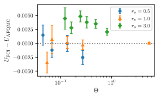
Figure 1: Comparison of ph-FT-AFQMC internal energies ($E_{h}$) to exact (FCI) results as a function of temperature for $\bar{N}=2$ for different values of $r_{s}$ and $M=7$.

The results of this comparison are plotted in Fig. 1 where we compare to a small system size ($\bar{N}=2$) as a function of $r_{s}$ and $\Theta$. At first look the figure looks reasonable: ph-FT-AFQMC agrees with FT-FCI very well for low $r_{s}$ (high densities) which is consistent with results at zero temperature,(Lee et al., 2019) and the results disagree more as $r_{s}$ increases and as the temperature decreases. Since the $T=0$ ph-ZT-AFQMC results are essentially exact for this system at all $r_{s}$ values considered here, this results unfortunately are a manifestation of the discrepancy between ph-FT-AFQMC and ph-ZT-AFQMC at the zero-temperature limit. For example at $r_{s}=3$ and $T=0$ the ph-ZT-AFQMC energy is -0.23968(3) $E_{h}/e$ which is statistically identical to the FCI result of -0.23968 $E_{h}/e$. This suggests that the phaseless constraint at finite temperature differs from that at zero temperature, and that it is potentially considerably larger.

In Section II.1.3, we analytically showed that two factors (constraint and chemical potential) can make the zero-temperature limit unreachable using the ph-FT-AFQMC algorithm. Incorporating other observations made in prior works,He et al. (2019a) we mention a total of four possible reasons for this disagreement:

1. the issue of chemical potential mismatch Since we work in different ensembles (FT with the grand canonical ensemble and ZT with the canonical ensemble), it is important to tune $\mu$ and $\mu_{T}$ properly so that the number of electrons does not fluctuate so much along an imaginary time path as assumed throughout the discussion in Section II.1.3. Based on Fig. 2, we suspect that this effect is quite minor since despite the fact that the average particle number deviates from the desired value along the path the effect of this deviation in other physical observables is negligible.

   

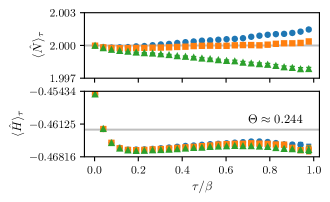
   Figure 2: Imaginary time dependence of the average electron number and total energy in ph-FT-AFQMC for the $r_{s}=3$, $N=2$, $M=7$ UEG model at $\beta=20$ $E_{\mathrm{h}}^{-1}$ or $\Theta\approx 0.244$ which is nearly the zero $T$ limit in this small supercell. The three different data sets correspond to 3 chemical potentials chosen around $\mu^{*}_{\mathrm{FCI}}$. In the lower panel the horizontal line represents the FCI total energy at this density. We used 2048 walkers, the pair-branch population control aglorithm, averaged over 30 independent simulations to obtain the error bars and used a timestep of 0.05 $E_{\mathrm{h}}^{-1}$.

   

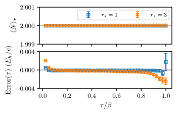
   Figure 3: Imaginary time dependence of the average electron number and error in the total energy ($u_{\mathrm{ph-FT-AFQMC}}(\tau)-u_{\mathrm{FCI}})$) in ph-FT-AFQMC for the $N=2$, $M=7$ UEG model for $r_{s}=1$ (blue squares) and $r_{s}=3$ (orange circles). For $r_{s}=1$ we chose $\beta=10$ $E_{\mathrm{h}}^{-1}$ ($\Theta\approx 0.05$) and for $r_{s}=3$ we chose $\beta=40$ $E_{\mathrm{h}}^{-1}$ ($\Theta\approx 0.122$). The temperatures were chosen such that they corresponded to the zero temperature limit. We used 2048 walkers, the pair-branch population control algorithm, averaged over 30 independent simulations to obtain the error bars and used a timestep of 0.05 $E_{\mathrm{h}}^{-1}$.

2. the fundamental differences between the two constraints A second possibility is that the constraints are fundamentally different even if $\mu$ and $\mu_{T}$ are chosen properly. This is then the direct consequence of the illustration suggested by Eq. 33 in Section II.1.3. Indeed as can be seen in Fig. 3 we see that this appears to be the case. Towards the end of the path we see that the ph-FT-AFQMC results begin to deviate substantially from the FCI result, with the magnitude of the deviation increasing with $r_{s}$. This is consistent with the fact that larger $r_{s}$ requires longer imaginary time to project out the ground state. This longer projection time results in a larger portion of the path using a determinant ratio that does not resemble the zero temperature overlap ratio. In the middle of the path results are close to exact and the algorithm more closely resembles ph-ZT-AFQMC.

3. the difference between trial density matrix and trial wavefunction A third possibility is that the FE trial density matrix is not appropriate to reproduce the correct zero temperature trial wavefunction used in ph-AFQMC. This is an important concern in general,(He et al., 2019a) however at the high densities and small systems sizes considered here we do not expect there to be any unrestricted Hartree–Fock solutions. Furthermore, for the UEG, RHF is equivalent to a free electron trial in a closed shell system. Nevertheless to verify this, we tested the thermal Hartree–Fock density matrix,(Mermin, 1963) however we see from Fig. 4 this choice makes essentially no practical difference.

   

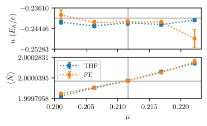
   Figure 4: Comparison between the ph-FT-AFQMC internal energy per electron $(u)$ and the average particle number as a function of the chemical potential with a free-electron (FE) and thermal Hartree–Fock (THF) like trial density matrix. The vertical (horizontal) lines represent the FCI values for the chemical potential (energy and electron number). The system considered here is $\bar{N}=2,M=7,r_{s}=3$ with $\beta=40E_{h}^{-1}$.

4. time-reversal symmetry breaking The final possibility is that as the phaseless constraint breaks imaginary time symmetry in the estimators,(He et al., 2019a) and we should instead average across time slices as suggested in Ref.50. Interestingly we find that at $r_{s}=3$ this averaging procedure biases results to be above the exact value (see Fig. 5), and again does not resolve this discrepancy with the zero temperature algorithm. This bias can also be understood in the context of Fig. 3 where the value of the energy along the imaginary time path is not symmetric with respect to $\tau$. While the time-averaged estimators were found to be more accruate in the Hubbard model,He et al. (2019a) given our results one should not expect this to be a general solution to this problem.

   

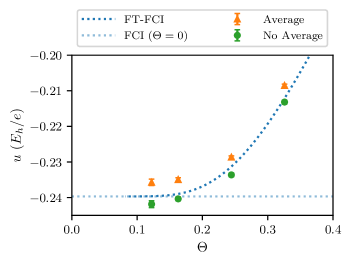
   Figure 5: Comparison between time slice averaged energies and the normal asymmetric estimator for the $M=7$, $\bar{N}=2$, $r_{s}=3$ benchmark system. Error bars where not visible are smaller that the markers. “No Average” refers to calculations where the global energy estimate is computed at $\tau=\beta$ where “Average” averages the global estimate across different time slices as suggested in ref. 50.

Despite these concerns it is also clear from Fig. 1 that ph-FT-AFQMC performs quite well with only small deviations seen from exact result in the regimes we are interested in (i.e., $\Theta<1$ and $r_{s}<3$).

IV.1.2 A study of $\bar{N}=66$ with $M=57$

We now study a larger UEG supercell considering $\bar{N}=66$ with $M=57$. Obviously, such a parameter set-up would have a very large basis set incompleteness error and therefore should not be used to draw any physically meaningful results. Nevertheless, for this basis set size, FT-CCSD results are available for several $\Theta$ and $r_{s}$ values (White and Chan, 2018) to which we compare ph-FT-AFQMC results. We use the FE trial density matrix as before since we do not have any UHF solutions at zero-temperature below $r_{s}=3$ as shown in Section VIII.1.

The result of this comparison is shown in Fig. 6. We see that ph-FT-AFQMC agrees well with FT-CCSD for low $r_{s}$ in all temperatures considered here. As we observed in the study of $\bar{N}=2$, the performance of ph-FT-AFQMC at low temperature may not be as good as the ph-ZT-AFQMC in the zero temperature limit. Nonetheless, we found accurate results at low $r_{s}$ in the case of $\bar{N}=2$ and we observe consistently accurate results at a larger supercell ($\bar{N}=66$) when compared against FT-CCSD. CCSD was shown to be accurate for low $r_{s}$ such as $r_{s}=0.5$ in the zero temperature benchmarkNeufeld and Thom (2017) so this helps us build confidence on the performance of ph-FT-AFQMC at low $r_{s}$.

However, the quality of FT-CCSD is expected to gradually degrade as $r_{s}$ increases and $\Theta$ decreases as indicated by its zero temperature benchmark study.Neufeld and Thom (2017) Consequently, at $r_{s}=4$ FT-CCSD exchange-correlation energies show erratic behavior changing the energy trend as a function of $r_{s}$ completely. ph-FT-AFQMC, on the other hand, shows a smooth monotonic behavior as a function of $r_{s}$ in all temperatures. Given the superior performance of ph-ZT-AFQMC compared to CCSD in the UEG model,Lee et al. (2019) this result is not surprising.

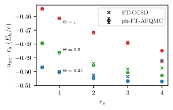
Figure 6: Comparison between ph-FT-AFQMC and FT-CCSD exchange-correlation energies as a function of temperature for $\bar{N}=66$, $M=57$. FT-CCSD energies are reproduced from Ref.37.

IV.2 Efficacy of the Low-Rank Truncation

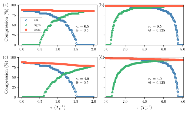
Figure 7: Demonstration of low-rank compression efficiency (%) in left, right, and total blocks for (a) $r_{s}=0.5$ and $\Theta=0.5$, (b) $r_{s}=0.5$ and $\Theta=0.125$, (c) $r_{s}=4.0$ and $\Theta=0.5$, and (d) $r_{s}=4.0$ and $\Theta=0.125$. All calculations are done with $M=1189$ and $\mu$ was chosen so that the one-body trial density matrix satisfies $\bar{N}=14$. A threshold of $10^{-6}$ was used in Eq. 54.

In Fig. 7, we show the practical effectiveness of the low-rank truncation discussed in Section II.4. We evaluate the compression percentage based on the ratio between the rank of left ($m_{L}$), right ($m_{R}$), and total ($m_{T}$) and the number of basis functions ($M$). Namely,

$$c_{i}=\left(1-\frac{m_{i}}{M}\right)\times 100\%$$ (78)

where $i\in\{L,R,T\}$. The set of parameters that we chose to look at this is $\bar{N}\simeq 14$, $M=1189$, $r_{s}=0.5,4.0$, and $\Theta=0.5,0.125$. For the purpose of demonstration, tuning chemical potential is not important so we set $\mu=\mu_{T}$ which ensures a correct average number of particles in the trial density matrix.

Comparing Fig. 7 (a) and (b), we see the effect of the temperature change at $r_{s}=0.5$. As expected the lower the temperature, we observe the higher compression ratio. In fact, we are in the limit where $M\gg\bar{N}$ so the low-rank compression becomes very effective. As we move along an imaginary path, we see that the compression efficiency decreases for left (trial density matrix blocks) and increases for right (sampled blocks). This is the feature of our propagation algorithm, which replaces $\hat{B}_{T}$ by $\hat{B}$ each time step. We observe nearly constant compression efficiency for the total block. We obtain about 80% compression in $m_{T}$ at $\Theta=0.5$ and nearly 100% compression in $m_{T}$ at $\Theta=0.125$. A similar conclusion can be drawn from Fig. 7 (c) and (d). We see only small changes in the compression efficiency when changing from $r_{s}=0.5$ to $r_{s}=4.0$.

While this technique is useful in speeding up the calculation in general, one needs a small $\bar{N}/M$ ratio and low temperature for a large saving. In our work, among larger calculations, the biggest saving was made in the case of $\bar{N}=66$ and $M=485$ at $\Theta=0.125$, which will be presented below. For this particular example, we did not find the cost saving to be substantial due to its sizable $\bar{N}/M$, but the compression algorithm was still used for the numerical stability.

IV.3 Comparison to Other Approaches

In Section IV.1, we focused on assessing the accuracy of ph-FT-AFQMC on a very small supercell for a given finite basis set. The results from Section IV.1 suggest that ph-FT-AFQMC is quite accurate for $r_{s}\leq 3$ and it is now important to assess the utility of this method in more realistic calculations specifically towards the CBS limit.

In Fig. 8 we investigate the magnitude of the basis set error as a function of $r_{s}$ at $\Theta=0.5$ where there exist previous exact CPIMC results as well as RPIMC data. We see that the ph-FT-AFQMC results are indistinguishable from the CPIMC results at $r_{s}=0.5$ when for $M\geq 257$ on the plotted scale. We also see that $M=485$ is sufficient to converge results up to $r_{s}=2$ on this scale. As seen in previous studies we find the RPIMC results to be too low, however the magnitude of this bias seems to decrease with increasing $r_{s}$. We can also ascribe the deviation of the FT-CCSD result from the PIMC data to the basis set size. We see that FT-CCSD and ph-FT-AFQMC agree well for $M=123$ (the largest basis set considered in Ref.38) up to $r_{s}=1$ with the FT-CCSD results deviating from the expected smooth trend with $r_{s}$ beyond this. Unfortunately we find obtaining ph-FT-AFQMC data beyond $r_{s}=2$ to be too expensive beyond $M=257$ due to the smaller timesteps required (equivalently the larger values of $\beta$ required as $r_{s}$ increases as in Eq. 76). Nevertheless the results look promising and it is possible that reliable results could be obtained for even larger $r_{s}$ values if more computational resources were expended.

With the confidence that the basis set error and phaseless error are under control in this parameter regime we next look towards the thermodynamic limit. To reach the thermodynamic limit we use finite size corrections calculated from the finite temperature random phase approximation.(Giuliani and Vignale, 2005; Tanaka and Ichimaru, 1986) The subject of finite size corrections is treated exhaustively elsewhere,(Groth et al., 2016; Malone, 2017; Dornheim et al., 2018a) and we will not discuss them in any detail. In essence, we add a correction $\Delta u_{\mathrm{xc}}(r_{s},\Theta,N)$ to our QMC results where

$$\Delta u_{\mathrm{xc}}(r_{s},\Theta,N)=u_{\mathrm{xc}}^{\mathrm{RPA}}(r_{s},\Theta,\infty)-u_{\mathrm{xc}}^{\mathrm{RPA}}(r_{s},\Theta,N),$$ (79)

where $u_{\mathrm{xc}}^{\mathrm{RPA}}$ can be computed numerically through derivatives of the exchange-correlation free energy. Detailed equations and the code necessary for this are available in Refs. 100 and 101. We also verified the accuracy of these corrections across $r_{s}$ and $\Theta\geq 1$ independently in our Supplementary Material(sup, ) using existing CPIMC and PB-PIMC data.(Dornheim et al., 2016a)

In Fig. 9 we compare our finite size corrected ph-FT-AFQMC results with $M=485$ to the fit of Ref.67 denoted here as GDSMFB and the RPIMC data of Ref.63. For $r_{s}<2.0$, we find excellent agreement between our data and the GDSMFB fit which is reassuring as the GDSMFB fit was generated using QMC data for the interaction energy, not the internal energy, and also relied exclusively on finite temperature PIMC data above $\Theta=0.5$, with a correction being applied to bridge the gap to the known zero temperature result.(Ceperley and Alder, 1980; Spink et al., 2013) We also compare to the KSDT fit from Karasiev et al. which was originally fitted to the RPIMC data and subsequently reparametrized(Karasiev et al., 2018) (corrKSDT) to correct the zero temperature limit and incorporate the more accurate CPIMC and PB-PIMC data from Ref.75. Similarly to previous work(Groth et al., 2017a; Karasiev et al., 2018) we find excellent agreement between our QMC data and GDSMFB and corrKSDT while we see some slight deviations at $\Theta=0.25$ from the KSDT fit. Note that we applied the same size corrections to the ph-FT-AFQMC and RPIMC data points and not the original size-corrections from Ref.63 which were subsequently found to be incorrect.(Groth et al., 2016) Thus the RPIMC data do not generally agree with the parameterizations. Lastly, we note that we observe a visible deviation of the ph-FT-AFQMC energy from the fits at $\Theta=0.5$ and $r_{s}=3$, which can be attributed to phaseless constraint bias and basis set incompleteness error.

The agreement between ph-FT-AFQMC and the GDSMFB fit gives added confidence that this procedure was well founded and the fit of GDSMFB is highly accurate particularly in the warm dense matter regime ($\Theta\leq 0.5$ and $r_{s}\leq 2$). Similar to other studies(Schoof et al., 2015b; Malone et al., 2016; Dornheim et al., 2016a) we find the RPIMC data is biased and generally too low, however this bias becomes small past $r_{s}=4$. We emphasize that in this parameter regime previously no other methods than RPIMC could run and no reliable verification of the GDSMFB fit was available. This gives us confidence that the ph-FT-AFQMC method will be useful for ab-initio simulations of warm-dense matters in the future.

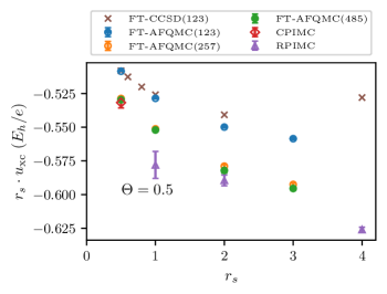
Figure 8: Basis set convergence of the ph-AFQMC exchange-correlation ($u_{\text{xc}}$) energy at $\Theta=0.5$, $\bar{N}=66$. CPIMC results were converged to the basis limit.(Dornheim et al., 2016a)

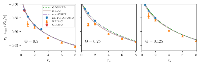
Figure 9: Comparison between finite size corrected ph-FT-AFQMC (with $M=485$), RPIMC(Brown et al., 2013b) and CPIMC(Dornheim et al., 2016a) exchange correlation energies $u_{\mathrm{xc}}$ to the GDSMFB fit,(Groth et al., 2017a) the KSDT fit,(Karasiev et al., 2014) and the corrected KSDT fit (corrKSDT).(Karasiev et al., 2018) Note no twist averaging was performed.

Finally, to assess the reliability of ph-FT-AFQMC for the calculation of properties other than the total energy we investigated the accuracy of the static structure factor

$$S(\mathbf{K})=\frac{1}{N}\langle\hat{\rho}(\mathbf{K})\hat{\rho}(-\mathbf{K})\rangle.$$ (80)

In Fig. 10 we compare our ph-FT-AFQMC results to the splined (exact) PB-PIMC and CPIMC results of Ref.71 where we find excellent agreement across $r_{s}$ at $\Theta=1$ which is the lowest temperature for which results exist.

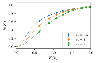
Figure 10: ph-FT-AFQMC static structure factor for the $\bar{N}=34$ electron gas at $\Theta=1$ (markers) compared to the unbiased splined PIMC results (dashed lines) from Ref. 71. The $K=0$ point has been omitted.

V Conclusions

In this work, we have examined the accuracy of phaseless finite temperature auxiliary-field quantum Monte Carlo (ph-FT-AFQMC) on the uniform electron gas (UEG) model over various Wigner-Seitz radii $r_{s}$ and temperatures $\Theta$. The ultimate goal of this work was to access the regime where $\Theta\leq 0.5$ and $r_{s}\leq 2.0$. This is the regime where other commonly used QMC methods such as configuration path integral MC (CPIMC) and permutation blocking PIMC (PB-PIMC) cannot be easily run. Furthermore, another popular flavor of QMC, restricted PIMC (RPIMC), typically exhibits a large bias for $r_{s}\leq 2.0$, which is currently the only many-body calculations available in this regime.

We summarize the findings and conclusions of our work as follows:

1. difficulties in reaching the accuracy of the zero temperature ph-AFQMC (ph-ZT-AFQMC) algorithm We showed both analytically and numerically that one should not expect the ph-FT-AFQMC energy to match the ph-ZT-AFQMC energy in the low-temperature limit even when the number of particles is tuned properly.

2. utility of low-rank truncation We demonstrated that the low-rank truncation method discussed in Ref. 85 is effective in the UEG Hamiltonian as well especially when $\Theta<0.5$.

3. accuracy of ph-FT-AFQMC energies We were able to use the ph-FT-AFQMC reliably to investigate $\Theta\leq 0.5$ and $r_{s}\leq 2.0$. Given the benchmark results on small basis sets that compare favorably to finite temperature coupled cluster with singles and doubles (FT-CCSD), ph-FT-AFQMC energies are expected to be accurate for a given basis set. Furthermore, we were able to run a large enough basis set so that the basis set incompleteness error is insignificant for the purpose of our study. Our work suggests that the bias in RPIMC is not negligible for $r_{s}<2$ and therefore one must be cautious when using RPIMC for dense electron gas simulations as previously suggested by others.(Schoof et al., 2015b; Malone et al., 2016; Dornheim et al., 2016a)

4. validation of the GDSMFB fit Groth et al. (2017a) of the exchange-correlation energies at difficult parameter regimes In the regime of $r_{s}\leq 2.0$ and $\Theta\leq 0.5$, no many-body methods have been able to verify the GDSMFB fit whose parametrization relies on the unbiased PIMC data for $\Theta\geq 0.5$. We found an excellent agreement between the GDSMFB fit and our ph-FT-AFQMC results.

5. accuracy of ph-FT-AFQMC static structure factors One benefit of working directly in the second-quantized space is to be able to compute properties straightforwardly. As an example, we computed the static structure factor of a super cell of $\bar{N}=34$ and compared our results to the numerical exact PIMC results. We found a nearly perfect agreement between ph-FT-AFQMC and PIMC.

Given our results, we are cautiously optimistic that ph-FT-AFQMC is a useful tool that is more scalable than other many-body methods based on the second quantization and can provide accurate results for the regimes where other methods either cannot run at all or cannot perform well.

However, the remaining issues in ph-FT-AFQMC should not be ignored. Most notably, the inability to access the same zero temperature limit as ph-ZT-AFQMC may become a more serious issue in the future since ph-ZT-AFQMC has been shown to be accurate in many benchmark systems. In light of Eq. 33 and Ref. 54, it will be interesting to investigate different types of constraints in the canonical ensemble which can guarantee the same zero temperature limit as ph-ZT-AFQMC.

Furthermore, reaching the basis set limit for higher temperature than $\Theta=1.0$ is excruciating even though the imaginary time propagation is short. Since there is no more obvious low-rank structure in the propagator, there seems not much that can be done to speed up. Nevertheless, given the exceptional speed-up shown by the ph-ZT-AFQMC implementation for solids using graphics processing units (GPUs),Malone et al. (2020b) we expect that the analogous ph-FT-AFQMC implementation using GPUs will help greatly to ameliorate this situation.

Looking to the future, one obvious extension will be to explore the dynamical structure factor which can be computed from analytically continued imaginary time displaced correlation functions in ph-FT-AFQMC.(Vitali et al., 2016; Motta et al., 2014, 2015) These results would build upon recent promising advances in the analytic continuation of PIMC data(Dornheim et al., 2018c; Groth et al., 2019b; Hamann et al., 2020) in the warm dense regime, where again we could potentially bridge the gap to lower temperatures. Another interesting avenue would be to explore to ability to compute free energy differences much like is done in interaction picture DMQMC(Malone et al., 2016). While the extension of ph-FT-AFQMC to Fermi-Bose mixtures when the number of bosons is conserved was presented,Rubenstein et al. (2012) it will be interesting to see further development for the cases with a non-conserving boson number.Lee et al. (2020c)

VI Acknowledgement

The work of J.L. was in part supported by the CCMS summer internship at the Lawrence Livermore National Lab in 2018. J.L. thanks Martin Head-Gordon and David Reichman for encouragement and support. We thank Hao Shi, Yuan-Yao He, and Shiwei Zhang for useful conversations on the FT-AFQMC algorithm. This work was performed under the auspices of the U.S. Department of Energy (DOE) by LLNL under Contract No. DE-AC52-07NA27344. The work of F. D. M and M. A. M. was supported by the U.S. DOE, Office of Science, Basic Energy Sciences, Materials Sciences and Engineering Division, as part of the Computational Materials Sciences Program and Center for Predictive Simulation of Functional Materials (CPSFM). Computing support for this work came from the LLNL Institutional Computing Grand Challenge program.

VII Data availability

The data that supports the findings of this study are available within the article. Raw data is published through a Zenodo repository.zen (2020)

VIII Appendix

VIII.1 Symmetry Breaking at Zero Temperature

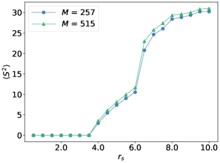
Figure 11: Spin expectation value ($\langle S^{2}\rangle$) of UHF as a function of $r_{s}$ at $\Theta=0$ for the 66-electron supercell at $M=257$ and $M=515$.

We studied the instability of RHF to UHF for the 66-electron supercell at zero temperature using the algorithm presented in Ref. 61. In Fig. 11, we present the spin expectation value ($\langle S^{2}\rangle$) of UHF as a function of $r_{s}$. We found that there is no spin polarization occurs for $r_{s}<4.0$ at zero temperature. As the focus of this study was the 66-electron supercell model for $r_{s}\leq 4.0$, we did not consider UHF trial density matrices. Since spin polarization is only small at $r_{s}=4.0$ and no spin polarization occurs for $r_{s}<4.0$ at zero temperature, it is expected that spin polarization would not occur at $T>0$, justifying our choice of the free-electron trial density matrix in this study.

References

- Petrov et al. (2003) D. S. Petrov, M. A. Baranov, and G. V. Shlyapnikov, Phys. Rev. A 67, 031601 (2003).
- Qin et al. (2020) M. Qin, C.-M. Chung, H. Shi, E. Vitali, C. Hubig, U. Schollwöck, S. R. White, and S. Zhang (Simons Collaboration on the Many-Electron Problem), Phys. Rev. X 10, 031016 (2020).
- Mukherjee et al. (2013) S. Mukherjee, F. Libisch, N. Large, O. Neumann, L. V. Brown, J. Cheng, J. B. Lassiter, E. A. Carter, P. Nordlander, and N. J. Halas, Nano Lett. 13, 240 (2013).
- Graziani (2014) F. Graziani, Frontiers and Challenges in Warm Dense Matter, Vol. 96 (Springer Science & Business, 2014).
- Fortney et al. (2009) J. J. Fortney, S. H. Glenzer, M. Koenig, B. Militzer, D. Saumon, and D. Valencia, Phys. Plasmas 16, 041003 (2009).
- Koenig et al. (2005) M. Koenig, A. Benuzzi-Mounaix, A. Ravasio, T. Vinci, N. Ozaki, S. Lepape, D. Batani, G. Huser, T. Hall, D. Hicks, A. MacKinnon, P. Patel, H. S. Park, T. Boehly, M. Borghesi, S. Kar, and L. Romagnani, Plasma Phys. Control. Fusion 47, B441 (2005).
- Ernstorfer et al. (2009) R. Ernstorfer, M. Harb, C. T. Hebeisen, G. Sciaini, T. Dartigalongue, and R. J. D. Miller, Science 323, 1033 (2009).
- Mermin (1965) N. D. Mermin, Phys. Rev. 137, A1441 (1965).
- Driver et al. (2015) K. P. Driver, F. Soubiran, S. Zhang, and B. Militzer, J. Chem. Phys. 143, 164507 (2015).
- Zhang et al. (2016) S. Zhang, K. P. Driver, F. Soubiran, and B. Militzer, High Energy Density Phys. 21, 16 (2016).
- Zhang et al. (2017) S. Zhang, K. P. Driver, F. Soubiran, and B. Militzer, J. Chem. Phys. 146, 074505 (2017).
- Driver et al. (2017) K. Driver, F. Soubiran, S. Zhang, and B. Militzer, High Energy Density Phys. 23, 81 (2017).
- Karasiev et al. (2016) V. V. Karasiev, L. Calderín, and S. B. Trickey, Phys. Rev. E 93, 063207 (2016).
- Karasiev et al. (2019) V. V. Karasiev, S. X. Hu, M. Zaghoo, and T. R. Boehly, Phys. Rev. B 99, 214110 (2019).
- Ramakrishna et al. (2020) K. Ramakrishna, T. Dornheim, and J. Vorberger, Phys. Rev. B 101, 195129 (2020).
- Mihaylov et al. (2020) D. I. Mihaylov, V. V. Karasiev, and S. X. Hu, Phys. Rev. B 101, 245141 (2020).
- Ceperley (1995) D. M. Ceperley, Rev. Mod. Phys. 67, 279 (1995).
- Ceperley (1991) D. M. Ceperley, J. Stat. Phys. 63, 1237 (1991).
- Foulkes et al. (2001) W. M. C. Foulkes, L. Mitas, R. J. Needs, and G. Rajagopal, Rev. Mod. Phys. 73, 33 (2001).
- Brown et al. (2013a) E. W. Brown, B. K. Clark, J. L. DuBois, and D. M. Ceperley, Phys. Rev. Lett. 110, 146405 (2013a).
- Schoof et al. (2015a) T. Schoof, S. Groth, J. Vorberger, and M. Bonitz, Phys. Rev. Lett. 115, 130402 (2015a).
- Malone et al. (2016) F. D. Malone, N. Blunt, E. W. Brown, D. Lee, J. Spencer, W. Foulkes, and J. J. Shepherd, Phys. Rev. Lett. 117, 115701 (2016).
- (23) J. L. DuBois, E. W. Brown, and B. J. Alder, “Overcoming the fermion sign problem in homogeneous systems,” in Advances in the Computational Sciences, Chap. 13, pp. 184–192.
- Dornheim et al. (2015) T. Dornheim, S. Groth, A. Filinov, and M. Bonitz, New J. Phys. 17, 73017 (2015).
- Schoof et al. (2011) T. Schoof, M. Bonitz, A. Filinov, D. Hochstuhl, and J. W. Dufty, Contr. Plasma Phys. 51, 687 (2011).
- Yilmaz et al. (2020) A. Yilmaz, K. Hunger, T. Dornheim, S. Groth, and M. Bonitz, J. Chem. Phys. 153, 124114 (2020).
- Blunt et al. (2014) N. S. Blunt, T. W. Rogers, J. S. Spencer, and W. M. C. Foulkes, Phys. Rev. B 89, 245124 (2014).
- Malone et al. (2015) F. D. Malone, N. S. Blunt, J. J. Shepherd, D. K. K. Lee, J. S. Spencer, and W. M. C. Foulkes, J. Chem. Phys. 143, 044116 (2015).
- Petras et al. (2020) H. R. Petras, S. K. Ramadugu, F. D. Malone, and J. J. Shepherd, J. Chem. Theory Comput. 16, 1029 (2020).
- Blunt et al. (2015) N. Blunt, A. Alavi, and G. H. Booth, Phys. Rev. Lett. 115 (2015).
- Dornheim et al. (2017a) T. Dornheim, S. Groth, F. D. Malone, T. Schoof, T. Sjostrom, W. M. C. Foulkes, and M. Bonitz, Phys. Plasmas 24, 056303 (2017a).
- He et al. (2014) X. He, S. Ryu, and S. Hirata, J. Chem. Phys. 140, 024702 (2014).
- Santra and Schirmer (2017) R. Santra and J. Schirmer, Chem. Phys. 482, 355 (2017).
- Hirata and Jha (2020) S. Hirata and P. K. Jha, J. Chem. Phys. 153, 014103 (2020).
- Jha and Hirata (2020) P. K. Jha and S. Hirata, Phys. Rev. E 101, 022106 (2020).
- Hermes and Hirata (2015) M. R. Hermes and S. Hirata, J. Chem. Phys. 143, 102818 (2015).
- White and Chan (2018) A. F. White and G. K.-L. Chan, J. Chem. Theory Comput. 14, 5690 (2018).
- White and Chan (2020) A. F. White and G. K.-L. Chan, J. Chem. Phys. 152, 224104 (2020).
- Harsha et al. (2019) G. Harsha, T. M. Henderson, and G. E. Scuseria, J. Chem. Phys. 150, 154109 (2019).
- Blankenbecler et al. (1981) R. Blankenbecler, D. J. Scalapino, and R. L. Sugar, Phys. Rev. D 24, 2278 (1981).
- Scalapino and Sugar (1981) D. J. Scalapino and R. L. Sugar, Phys. Rev. Lett. 46, 519 (1981).
- Zhang and Krakauer (2003) S. Zhang and H. Krakauer, Phys. Rev. Lett. 90, 136401 (2003).
- Zhang (1999) S. Zhang, Phys. Rev. Lett. 83, 2777 (1999).
- LeBlanc et al. (2015) J. P. F. LeBlanc, A. E. Antipov, F. Becca, I. W. Bulik, G. K.-L. Chan, C.-M. Chung, Y. Deng, M. Ferrero, T. M. Henderson, C. A. Jiménez-Hoyos, E. Kozik, X.-W. Liu, A. J. Millis, N. V. Prokof’ev, M. Qin, G. E. Scuseria, H. Shi, B. V. Svistunov, L. F. Tocchio, I. S. Tupitsyn, S. R. White, S. Zhang, B.-X. Zheng, Z. Zhu, and E. Gull (Simons Collaboration on the Many-Electron Problem), Phys. Rev. X 5, 041041 (2015).
- Motta et al. (2017) M. Motta, D. M. Ceperley, G. K.-L. Chan, J. A. Gomez, E. Gull, S. Guo, C. A. Jiménez-Hoyos, T. N. Lan, J. Li, F. Ma, et al., Phys. Rev. X 7, 031059 (2017).
- Williams et al. (2020) K. T. Williams, Y. Yao, J. Li, L. Chen, H. Shi, M. Motta, C. Niu, U. Ray, S. Guo, R. J. Anderson, J. Li, L. N. Tran, C.-N. Yeh, B. Mussard, S. Sharma, F. Bruneval, M. van Schilfgaarde, G. H. Booth, G. K.-L. Chan, S. Zhang, E. Gull, D. Zgid, A. Millis, C. J. Umrigar, and L. K. Wagner (Simons Collaboration on the Many-Electron Problem), Phys. Rev. X 10, 011041 (2020).
- Lee et al. (2020a) J. Lee, F. D. Malone, and D. R. Reichman, J. Chem. Phys. 153, 126101 (2020a).
- Lee et al. (2020b) J. Lee, F. D. Malone, and M. A. Morales, J. Chem. Theory Comput. 16, 3019 (2020b).
- Malone et al. (2020a) F. D. Malone, A. Benali, M. A. Morales, M. Caffarel, P. R. C. Kent, and L. Shulenburger, Phys. Rev. B 102, 161104 (2020a).
- He et al. (2019a) Y. Y. He, M. Qin, H. Shi, Z. Y. Lu, and S. Zhang, Phys. Rev. B 99, 045108 (2019a).
- Rubenstein et al. (2012) B. M. Rubenstein, S. Zhang, and D. R. Reichman, Phys. Rev. A 86, 053606 (2012).
- Liu et al. (2018) Y. Liu, M. Cho, and B. Rubenstein, J. Chem. Theory Comput. 14, 4722 (2018).
- Liu et al. (2020) Y. Liu, T. Shen, H. Zhang, and B. Rubenstein, J. Chem. Theory Comput. 16, 4298 (2020).
- Shen et al. (2020) T. Shen, Y. Liu, Y. Yu, and B. M. Rubenstein, J. Chem. Phys. 153, 204108 (2020).
- Lee and Reichman (2020) J. Lee and D. R. Reichman, J. Chem. Phys. 153, 044131 (2020).
- Malone et al. (2019) F. D. Malone, S. Zhang, and M. A. Morales, J. Chem. Theory Comput. 15, 256 (2019).
- Giuliani and Vignale (2005) G. Giuliani and G. Vignale, Quantum theory of the electron liquid (Cambridge university press, 2005).
- Ceperley and Alder (1980) D. M. Ceperley and B. J. Alder, Phys. Rev. Lett. 45, 566 (1980).
- Perdew and Zunger (1981) J. P. Perdew and A. Zunger, Phys. Rev. B 23, 5048 (1981).
- Perdew et al. (1996) J. P. Perdew, K. Burke, and M. Ernzerhof, Phys. Rev. Lett. 77, 3865 (1996).
- Lee et al. (2019) J. Lee, F. D. Malone, and M. A. Morales, J. Chem. Phys. 151, 064122 (2019).
- Dornheim et al. (2018a) T. Dornheim, S. Groth, and M. Bonitz, Phys. Rep. 744, 1 (2018a).
- Brown et al. (2013b) E. W. Brown, B. K. Clark, J. L. DuBois, and D. M. Ceperley, Phys. Rev. Lett. 110, 146405 (2013b).
- Schoof et al. (2015b) T. Schoof, S. Groth, J. Vorberger, and M. Bonitz, Phys. Rev. Lett. 115, 130402 (2015b).
- Brown et al. (2013c) E. W. Brown, J. L. DuBois, M. Holzmann, and D. M. Ceperley, Phys. Rev. B 88, 081102 (2013c).
- Karasiev et al. (2014) V. V. Karasiev, T. Sjostrom, J. Dufty, and S. B. Trickey, Phys. Rev. Lett. 112, 076403 (2014).
- Groth et al. (2017a) S. Groth, T. Dornheim, T. Sjostrom, F. D. Malone, W. M. Foulkes, and M. Bonitz, Phys. Rev. Lett. 119, 135001 (2017a).
- Groth et al. (2016) S. Groth, T. Schoof, T. Dornheim, and M. Bonitz, Phys. Rev. B 93, 085102 (2016).
- Dornheim et al. (2016a) T. Dornheim, S. Groth, T. Schoof, C. Hann, and M. Bonitz, Phys. Rev. B 93, 205134 (2016a).
- Dornheim et al. (2017b) T. Dornheim, S. Groth, J. Vorberger, and M. Bonitz, Phys. Rev. E 96, 023203 (2017b).
- Dornheim et al. (2017c) T. Dornheim, S. Groth, and M. Bonitz, Contrib. to Plasma Phys. 57, 468 (2017c).
- Groth et al. (2017b) S. Groth, T. Dornheim, and M. Bonitz, J. Chem. Phys. 147, 164108 (2017b).
- Dornheim et al. (2018b) T. Dornheim, S. Groth, J. Vorberger, and M. Bonitz, Phys. Rev. Lett. 121, 255001 (2018b).
- Groth et al. (2019a) S. Groth, T. Dornheim, and J. Vorberger, Phys. Rev. B 99, 235122 (2019a).
- Dornheim et al. (2016b) T. Dornheim, S. Groth, T. Sjostrom, F. D. Malone, W. M. C. Foulkes, and M. Bonitz, Phys. Rev. Lett. 117, 156403 (2016b).
- Hubbard (1959) J. Hubbard, Phys. Rev. Lett. 3, 77 (1959).
- Hirsch (1985) J. E. Hirsch, Phys. Rev. B 31, 4403 (1985).
- Dos Santos (2003) R. R. Dos Santos, “Introduction to Quantum Monte Carlo simulations for fermionic systems,” (2003).
- Bruus and Flensberg (2004) H. Bruus and K. Flensberg, Many-body quantum theory in condensed matter physics: an introduction (Oxford university press, 2004).
- Wilson and Gyorffy (1995) M. T. Wilson and B. L. Gyorffy, J. Phys. Condens. Matter 7, L371 (1995).
- Loh and Gubernatis (1992) E. Loh and J. Gubernatis (Elsevier, 1992) pp. 177–235.
- Purwanto et al. (2009) W. Purwanto, H. Krakauer, and S. Zhang, Phys. Rev. B 80, 214116 (2009).
- White et al. (1989) S. R. White, D. J. Scalapino, R. L. Sugar, E. Y. Loh, J. E. Gubernatis, and R. T. Scalettar, Phys. Rev. B 40, 506 (1989).
- Tomas et al. (2012) A. Tomas, C.-C. Chang, R. Scalettar, and Z. Bai, in IPDPS (2012) pp. 308–319.
- He et al. (2019b) Y.-Y. He, H. Shi, and S. Zhang, Phys. Rev. Lett. 123, 136402 (2019b).
- Suewattana et al. (2007) M. Suewattana, W. Purwanto, S. Zhang, H. Krakauer, and E. J. Walter, Phys. Rev. B 75, 245123 (2007).
- Zhang and Ceperley (2008) S. Zhang and D. M. Ceperley, Phys. Rev. Lett. 100, 236404 (2008).
- (88) See https://github.com/pauxy-qmc/pauxy for details on how to obtain the source code.
- Spencer et al. (2019) J. S. Spencer, N. S. Blunt, S. Choi, J. Etrych, M.-A. Filip, W. M. C. Foulkes, R. S. T. Franklin, W. J. Handley, F. D. Malone, V. A. Neufeld, R. Di Remigio, T. W. Rogers, C. J. C. Scott, J. J. Shepherd, W. A. Vigor, J. Weston, R. Xu, and A. J. W. Thom, J. Chem. Theory Comput. 15, 1728 (2019).
- Spencer et al. (2015) J. S. Spencer, N. S. Blunt, W. A. Vigor, F. D. Malone, W. M. C. Foulkes, J. J. Shepherd, and A. J. W. Thom, J. Open Res. Softw. 3, 1 (2015).
- Shao et al. (2015) Y. Shao, Z. Gan, E. Epifanovsky, A. T. Gilbert, M. Wormit, J. Kussmann, A. W. Lange, A. Behn, J. Deng, X. Feng, D. Ghosh, M. Goldey, P. R. Horn, L. D. Jacobson, I. Kaliman, R. Z. Khaliullin, T. Kuś, A. Landau, J. Liu, E. I. Proynov, Y. M. Rhee, R. M. Richard, M. A. Rohrdanz, R. P. Steele, E. J. Sundstrom, H. L. Woodcock, P. M. Zimmerman, D. Zuev, B. Albrecht, E. Alguire, B. Austin, G. J. Beran, Y. A. Bernard, E. Berquist, K. Brandhorst, K. B. Bravaya, S. T. Brown, D. Casanova, C. M. Chang, Y. Chen, S. H. Chien, K. D. Closser, D. L. Crittenden, M. Diedenhofen, R. A. Distasio, H. Do, A. D. Dutoi, R. G. Edgar, S. Fatehi, L. Fusti-Molnar, A. Ghysels, A. Golubeva-Zadorozhnaya, J. Gomes, M. W. Hanson-Heine, P. H. Harbach, A. W. Hauser, E. G. Hohenstein, Z. C. Holden, T. C. Jagau, H. Ji, B. Kaduk, K. Khistyaev, J. Kim, J. Kim, R. A. King, P. Klunzinger, D. Kosenkov, T. Kowalczyk, C. M. Krauter, K. U. Lao, A. D. Laurent, K. V. Lawler, S. V. Levchenko, C. Y. Lin, F. Liu, E. Livshits, R. C. Lochan, A. Luenser, P. Manohar, S. F. Manzer, S. P. Mao, N. Mardirossian, A. V. Marenich, S. A. Maurer, N. J. Mayhall, E. Neuscamman, C. M. Oana, R. Olivares-Amaya, D. P. Oneill, J. A. Parkhill, T. M. Perrine, R. Peverati, A. Prociuk, D. R. Rehn, E. Rosta, N. J. Russ, S. M. Sharada, S. Sharma, D. W. Small, A. Sodt, T. Stein, D. Stück, Y. C. Su, A. J. Thom, T. Tsuchimochi, V. Vanovschi, L. Vogt, O. Vydrov, T. Wang, M. A. Watson, J. Wenzel, A. White, C. F. Williams, J. Yang, S. Yeganeh, S. R. Yost, Z. Q. You, I. Y. Zhang, X. Zhang, Y. Zhao, B. R. Brooks, G. K. Chan, D. M. Chipman, C. J. Cramer, W. A. Goddard, M. S. Gordon, W. J. Hehre, A. Klamt, H. F. Schaefer, M. W. Schmidt, C. D. Sherrill, D. G. Truhlar, A. Warshel, X. Xu, A. Aspuru-Guzik, R. Baer, A. T. Bell, N. A. Besley, J. D. Chai, A. Dreuw, B. D. Dunietz, T. R. Furlani, S. R. Gwaltney, C. P. Hsu, Y. Jung, J. Kong, D. S. Lambrecht, W. Liang, C. Ochsenfeld, V. A. Rassolov, L. V. Slipchenko, J. E. Subotnik, T. Van Voorhis, J. M. Herbert, A. I. Krylov, P. M. Gill, and M. Head-Gordon, Mol. Phys. 113, 184 (2015).
- Booth and Gubernatis (2009) T. E. Booth and J. E. Gubernatis, Phys. Rev. E 80, 046704 (2009).
- Nguyen et al. (2014) H. Nguyen, H. Shi, J. Xu, and S. Zhang, Comput. Phys. Commun. 185, 3344 (2014), 1407.7967 .
- Wagner et al. (2009) L. K. Wagner, M. Bajdich, and L. Mitas, J. Comput. Phys. 228, 3390 (2009).
- zen (2020) “Data for “a phaseless auxiliary-field quantum monte carlo perspective on the uniformelectron gas at finite temperatures: Issues, observations, and benchmark study”,” (2020).
- Kou and Hirata (2014) Z. Kou and S. Hirata, Theor. Chem. Acc. 133, 1487 (2014).
- Mermin (1963) N. D. Mermin, Ann. Phys. (N. Y). 21, 99 (1963).
- Neufeld and Thom (2017) V. A. Neufeld and A. J. W. Thom, J. Chem. Phys. 147, 194105 (2017).
- Tanaka and Ichimaru (1986) S. Tanaka and S. Ichimaru, J. Phys. Soc. of Jpn. 55, 2278 (1986).
- Malone (2017) F. D. Malone, Quantum Monte Carlo Simulations of Warm Dense Matter (Ph.D. thesis, Imperial College London, 2017) pp. 106–110.
- (101) See https://www.github.com/fdmalone/uegpy for details on how to obtain the source code., accessed: 2020-12-16.
- (102) See [URL BE INSERTED] for supplementary information.
- Spink et al. (2013) G. G. Spink, R. J. Needs, and N. D. Drummond, Phys. Rev. B 88, 085121 (2013).
- Karasiev et al. (2018) V. V. Karasiev, J. W. Dufty, and S. B. Trickey, Phys. Rev. Lett. 120, 076401 (2018).
- Malone et al. (2020b) F. D. Malone, S. Zhang, and M. A. Morales, J. Chem. Theory Comput. 16, 4286 (2020b).
- Vitali et al. (2016) E. Vitali, H. Shi, M. Qin, and S. Zhang, Phys. Rev. B 94, 085140 (2016).
- Motta et al. (2014) M. Motta, D. E. Galli, S. Moroni, and E. Vitali, J. Chem. Phys. 140, 024107 (2014).
- Motta et al. (2015) M. Motta, D. E. Galli, S. Moroni, and E. Vitali, J. Chem. Phys. 143, 164108 (2015).
- Dornheim et al. (2018c) T. Dornheim, S. Groth, J. Vorberger, and M. Bonitz, Phys. Rev. Lett. 121, 255001 (2018c).
- Groth et al. (2019b) S. Groth, T. Dornheim, and J. Vorberger, Phys. Rev. B 99, 235122 (2019b).
- Hamann et al. (2020) P. Hamann, T. Dornheim, J. Vorberger, Z. A. Moldabekov, and M. Bonitz, Phys. Rev. B 102, 125150 (2020).
- Lee et al. (2020c) J. Lee, S. Zhang, and D. R. Reichman, arXiv (2020c), 2012.13473 .