Kardar-Parisi-Zhang universality in two-component driven diffusive models: Symmetry and renormalization group perspectives

Abstract

We elucidate the universal spatio-temporal scaling properties of the time-dependent correlation functions in a class of two-component one-dimensional (1D) driven diffusive system that consists of two coupled asymmetric exclusion process. By using a perturbative renormalization group framework, we show that the relevant scaling exponents have values same as those for the 1D Kardar-Parisi-Zhang (KPZ) equation. We connect these universal scaling exponents with the symmetries of the model equations. We thus establish that these models belong to the 1D KPZ universality class.

I Introduction

Driven diffusive models are paradigmatic nonequilibrium models that display nonequilibrium universal scaling behavior different from any known dynamical scaling universality in equilibrium systems. One of the most well-known examples is the one-dimensional (1D) driven diffusive model ddlg that displays the Kardar-Parisi-Zhang (KPZ) universality class kpz . Subsequently, this has been generalized to a variety of multi-component driven diffusive models that yield a widely varying scaling behavior, ranging from continuously varying universality abmhd and weak dynamic scaling mustansir to strong dynamic scaling belonging to the KPZ universality class. In a recent study on the dynamical response to small distortions of a 1D lattice drifting through a dissipative medium about its uniform state, we show that the fluctuations, both transverse and longitudinal to the direction of the drift, exhibit strong dynamic scaling and belong to the KPZ universality class  ep_pre . In spite of these large bodies of studies, the general question of universality in 1D multi-variable driven diffusive systems remains open.

A particularly interesting class of models includes multi-species driven diffusive models that admit more than one conservation law. While there have been several studies in this context, a general consensus on the question of universality is still lacking. For instance, Ferrari et al. ferrari studied a two-species exclusion process by using a mode-coupling theory and Monte Carlo simulations, and found two very clean KPZ-modes, but no other modes. For a similar model, exact finite-size scaling analysis of the spectrum indicates a dynamical exponent $z=3/2$ arita , which is consistent with the 1D KPZ universality class. In earlier works on other lattice gas models with two conservation laws, the presence of a KPZ mode and a diffusive mode was claimed mustansir ; rakos , indicating weak dynamic scaling. In Ref. mustansir , this occurrence of weak dynamic scaling is shown to be connected to special symmetries for carefully chosen parameters and the associated kinematic waves; else only KPZ universality is observed. This opens a question on how robust or general is the KPZ universality in 1D driven diffusive systems. Furthermore, this opens up to a broader generic issue of the robustness of a universality class against non-existence of a nonlinear coefficient - when vanishing of a particular nonlinear coefficient can affect the universality class obtained with a non-zero value of it and when cannot, and how this is connected to the symmetry of the model. A classic example is the $\phi^{4}$ Landau-Ginzburg theory with a $u\phi^{4},\,u>0$ anharmonic term that describes the Ising model near its second order transition chaikin , where if we set $u=0$ identically, then the model becomes the Gaussian model, having critical exponents entirely different from the Ising model in the paramagnetic phase near the critical point, and in fact shows no phase transition chaikin . This opens the question whether a reverse scenario, where vanishing of a relevant (in the renormalization group or RG sense) nonlinear coefficient in a dynamical model can leave the universal scaling and the universality class unchanged. In the absence of any general framework to study this in nonequilibrium systems, it is useful to construct simple models and perform explicit calculations to investigate this issue. There have already been some studies in this context in versions of driven diffusive generalized Burgers models. For instance, Ref. popkov proposed and studied a two-species driven diffusive model and found a KPZ mode and a non-KPZ mode with dynamic exponent $z=5/3$ within a mode coupling theory and dynamic Monte Carlo simulations. Subsequently, Ref. spohn1 studied generalized coupled Burgers model and found the existence of a mode with $z=5/3$ in certain limits when some nonlinear coupling constants vanish by using mode coupling methods; see also Ref. spohn2 in this context. More recently, Ref. spohn3 revisited this generic class of coupled models and obtained within the framework of mode coupling theories one mode with $z=5/3$ in similar limits as the other previous related studies. Very recently, Schmidt et al van in a 1D three species model found two KPZ modes with $z=3/2$ and a third mode with $z=5/3$ by employing mode coupling methods and dynamical Monte Carlo simulations. The question that naturally arises is how or whether we can reconcile these results with the symmetry of the models.

In this work, we revisit this issue. We analyze a series of related two-species driven diffusive models popkov ; spohn1 ; ferrari ; van , and investigate the universal scaling properties of these models and their symmetries. We analyze the model in Ref. popkov in details by means of perturbative dynamic renormalization group (DRG) for our work, that is well-suited to extract universal scaling properties of dynamical models, and then extend this analysis to the models in Refs. spohn1 ; ferrari ; van .

Our DRG treatment emphatically shows that, contrary to recent claims  popkov , there are only two KPZ-like modes admitted by the model popkov , implying 1D KPZ universal behavior.

The rest of the article is organized as follows. In Sec. II, we describe the model. In Sec. III, we briefly discuss the KPZ equation and its universal properties at 1D. In Sec. IV, we set up the continuum equations that we study. We analyze the scaling properties of one particular case of the two-species model in Sec. V. Then in Sec. V.1, we present the DRG analysis of the model. In Sec. VI, we summarize. Some of the technical details are made available in Appendix for the interested reader.

II Multi-species models

We use the model studied in Ref. popkov ; which is a stochastic lattice gas model of two lanes where particles can hop randomly on two lanes. Each lane has $N$ sites. The model is defined as follows. Particles move unidirectionally but without exchanging the lane. Periodic boundary conditions are imposed on each chain. Particles can hop from site $k$ to $k+1$ if site $k+1$ is empty. Furthermore, $n_{k}^{(i)}$ is the particle occupation number on site $k$ in lane $i$ and the particle hopping rate $r_{i}$ in lane $i$ from site $k$ to $k+1$ depends on the occupation numbers on sites $k$ and $k+1$ in the adjacent lane. The hopping rates in the two lanes are given by

$$r_{1}=1+\gamma n^{(2)}/2,\,\,\,\,r_{2}=\tilde{b}+\gamma n^{(1)}/2\,,$$ (1)

where the coupling parameter $\gamma\geq-min(1,\tilde{b})$ and $n^{i}=n_{k}^{i}+n_{k+1}^{i}$  popkov  . This model reduces to the two lane model of  PopkovJstat for $\tilde{b}=1$. Total number of particles $M_{i}$ in each lane is conserved. Thus, there are two conservation laws in this model.

III Kardar-Parisi-Zhang equation

We briefly revisit the KPZ equation before embarking on our calculations. Consider a 1D model with periodic boundary condition having one type of particles only that execute asymmetric exclusion processes. In a coarse-grained description, the local density $\rho(x,t)$ is known to follow the Burgers equation fns , which in turn can be mapped onto the KPZ equation for a single-valued height field $h(x,t)$

$$\frac{\partial h}{\partial t}-\frac{\lambda}{2}(\partial_{x}h)^{2}=\nu\frac{\partial^{2}h}{\partial x^{2}}+\eta,$$ (2)

where $\rho(x,t)=-\partial_{x}h(x,t)$, and $\eta(x,t)$ is a zero-mean, Gaussian-distributed white noise. The correlator of $h$ shows universal spatio-temporal scaling in the long wavelength limit that are independent of the model parameters barabasi . In particular, in the Fourier space correlator

$$C_{h}(k,\omega)\sim\langle|h(k,\omega)|^{2}\rangle\sim q^{-1-2\chi_{h}}f_{h}(k^{z}/\omega).$$ (3)

Here, $k$ and $\omega$, respectively, are Fourier wavevector and frequency; $\chi_{h}$, the roughness exponent and $z$, the dynamic exponent, are the universal scaling exponent that characterise the universal scaling of $C_{h}(k,\omega)$; $f_{h}$ is a dimensionless scaling function.For 1D KPZ, these exponents are known exactly: $\chi_{h}=1/2$ and $z=3/2$ barabasi ; natter .

Consider now a hypothetical equation

$$\frac{\partial h}{\partial t}-\frac{\lambda_{4}}{2}(\partial_{x}h)^{4}=\nu\frac{\partial^{2}h}{\partial x^{2}}+\eta,$$ (4)

where $\lambda_{4}$ is a coupling constant. Equation (4) has the same symmetry as (2). However, by naive power counting leads to the conclusion that $\lambda_{4}$ is irrelevant in the RG sense, which then should give the linear theory scaling to be the asymptotic long wavelength limit scaling in this model. This is however wrong. One could write $(\partial_{x}h)^{4}=\langle(\partial_{x}h)^{2}\rangle(\partial_{x}h)^{2}$ to the leading order in fluctuations. This evidently generate a $(\partial_{x}h)^{2}$ in Eq. (4), ultimately making it statistically identical to Eq. (2) in the long wavelength limit. That a $(\partial_{x}h)^{2}$ is generated by fluctuations is not surprising, as (2) and (4) belong to the same symmetry. Thus the lesson we can draw from this example is that the mere presence or absence of a particular relevant nonlinear term cannot be directly used to infer the universal properties; one needs to take the symmetries into account and start by using the most general equation containing all possible symmetry-permitted relevant nonlinear terms.

IV Continuum equations of motion for the two-species model

In order to extract the universal scaling behavior of the two-species model, we take the continuum hydrodynamic approach that is particularly suitable to extract long wavelength universal scaling properties chaikin ; foster . In this approach, the equations of motion for the “hydrodynamic variables”, which have diverging relaxation times in the vanishing wavevector limits, are constructed in expansions in the fields and gradients, retaining all possible symmetry-permitted lowest order nonlinear terms. In the present study, the two conserved densities in the two lanes are the only hydrodynamic variables. we first consider the continuum coarse-grained equations of motion for the two densities in the two-species model. We begin by noting that the stationary currents in first and second lanes are (see Ref. popkov for details)

$$j_{1}(\rho_{1},\rho_{2}) = \rho_{1}(1-\rho_{1})(1+\gamma\rho_{2})\,,$$ (5)

$$j_{2}(\rho_{1},\rho_{2}) = \rho_{2}(1-\rho_{2})(b+\gamma\rho_{1}),$$ (6)

where $\rho_{i}=M_{i}/N$, $i=1,2$ are the particle densities in each lane  popkov  . Here $M_{i}$ is the number of particles on $i-$th lane and $N$ is the number of lattice sites in each lane. The coarse-grained local density $\rho_{i}(x,t)$ for component $i$ obey the continuity equation which can be written in a compact form as $\frac{\partial}{\partial t}{\rho_{i}}+A_{ij}\frac{\partial}{\partial x}{\rho_{j}}=0$  where $A$ is the Jacobian matrix with matrix elements $A_{ij}=\partial j_{i}/\partial\rho_{j}$. Local densities can be expanded around its stationary values: $\rho_{i}(x,t)=\rho_{i}+u_{i}(x,t)$ . The normal modes are ${\phi_{i}}=R_{ij}{u_{j}}$ where $RAR^{-1}=\,$diag$(v_{i})$ with $v_{i}$’s being the eigenvalues of $A$ to the lowest order in spatial gradients; these $v_{i}$’s are the characteristic velocities with which local perturbations move. The transformation matrix $R$ satisfies the normalization condition $RCR^{T}$=1 where $C$ is the compressibility matrix. Keeping the lowest order nonlinearities, the equations of motion of the normal modes are

$$\partial_{t}\phi_{i}=-\partial_{x}[v_{i}\phi_{i}+(1/2)\langle\vec{\phi},G^{(i)}\vec{\phi}\rangle-\partial_{x}(D\vec{\phi})_{i}+(B\vec{\eta})_{i}]$$ (7)

with $i=1,2$ . Here, $D$ and $B$ are transformed diffusion matrix and transformed noise strength matrix respectively. $\vec{\eta}$ is the noise vector. The mode coupling matrices, $G^{(i)}=(1/2)\sum_{j}R_{ij}(R^{-1})^{T}H^{(j)}R^{-1}$ depend on the Hessian matrix with elements $H^{(i)}=\partial^{2}j_{i}/(\partial\rho_{j}\partial\rho_{k})$ . The coupling matrices $G^{(i)}$ are

$$G^{(i)}=\left[\begin{array}[]{cc}G_{11}^{(i)}&G_{12}^{(i)}\\ G_{21}^{(i)}&G_{22}^{(i)}\end{array}\right].$$

In the equations of motion for $\phi_{1}$ and $\phi_{2}$ nonlinearities appear as an inner product $\langle\vec{\phi},G^{(i)}\vec{\phi}\rangle$ which can be expanded as

$$\langle\vec{\phi},G^{(i)}\vec{\phi}\rangle=\left[\begin{array}[]{cc}\phi_{1}&\phi_{2}\end{array}\right]\left[\begin{array}[]{cc}G_{11}^{(i)}&G_{12}^{(i)}\\ G_{21}^{(i)}&G_{22}^{(i)}\end{array}\right]\left[\begin{array}[]{c}\phi_{1}\\ \phi_{2}\end{array}\right]$$

$=G_{11}^{(i)}\phi_{1}^{2}+G_{12}^{(i)}\phi_{1}\phi_{2}+G_{21}^{(i)}\phi_{1}\phi_{2}+G_{22}^{(i)}\phi_{2}^{2}$ .

We consider the normal modes for constant particle densities $\rho_{1}=\rho_{2}=\rho$ in each lane and coupling parameter $\gamma=1$. The equations of motion for $\phi_{1}$ and $\phi_{2}$ are

$$\partial_{t}\phi_{1}={} -\partial_{x}(v_{1}\phi_{1})-\frac{1}{2}\partial_{x}[G_{11}^{(1)}\phi_{1}^{2}+(G_{12}^{(1)}+G_{21}^{(1)})\phi_{1}\phi_{2}$$ (8)

$$+G_{22}^{(1)}\phi_{2}^{2}]+D_{1}\partial_{x}^{2}\phi_{1}-\partial_{x}(B_{1}\eta_{1}),$$

$$\partial_{t}\phi_{2}={} -\partial_{x}(v_{2}\phi_{2})-\frac{1}{2}\partial_{x}[G_{11}^{(2)}\phi_{1}^{2}+(G_{12}^{(2)}+G_{21}^{(2)})\phi_{1}\phi_{2}$$ (9)

$$+G_{22}^{(2)}\phi_{2}^{2}]+D_{2}\partial_{x}^{2}\phi_{2}-\partial_{x}(B_{2}\eta_{2}).$$

We retain only the diagonal terms from the diffusion matrix since the pure diffusive terms have more dominant contributions than the cross diffusive terms to the eigenvalues (see Appendix for the details).

The above equations are decoupled at the linear level. We consider the case for which $\tilde{b}=2$ . In this case, the characteristic velocities are $v_{1}=1-\rho-3\rho^{2}$ and $v_{2}=2-3\rho-\rho^{2}$ . For $\tilde{b}=2$, $\gamma=1$, $\rho_{1}=\rho_{2}=\rho$ we can calculate the $G$ matrix using its definition above. The matrix elements of the coupling matrices are $G_{11}^{(1)}=-2g_{0}(6\rho^{4}-8\rho^{3}+5\rho^{2}+\rho-1)$ , $G_{12}^{(1)}=G_{21}^{(1)}=g_{0}(4\rho^{3}-10\rho^{2}+8\rho-1)$ , $G_{22}^{(1)}=-2g_{0}\rho(1-\rho)(2\rho^{2}-6\rho+3)$ and $G_{11}^{(2)}=4g_{0}\rho(1-\rho)$ , $G_{12}^{(2)}=G_{21}^{(2)}=-g_{0}(1-2\rho^{2})^{2}$ , $G_{22}^{(2)}=4g_{0}(1-3\rho(1-\rho))$ with $g_{0}=-\frac{1}{2}\left[\rho(1-\rho)/(1-2\rho(1-\rho))^{3}\right]^{1/2}$  popkov  . There are three possible cases depending on the mode coupling matrix.
${\bf{A.}}$ If $G_{11}^{(1)}$ and $G_{22}^{(2)}$ are nonzero then the equations for $\phi_{1}$ and $\phi_{2}$ are same as the above equations (8) and (9) . Now we make a change of variable $\phi_{1}=-\partial_{x}h_{1}$, $\phi_{2}=-\partial_{x}h_{2}$ and rewrite the above equations which will be of the form

$$\frac{\partial h_{1}}{\partial t}={} -v_{1}\frac{\partial h_{1}}{\partial x}+\frac{G_{11}^{(1)}}{2}(\frac{\partial h_{1}}{\partial x})^{2}+\frac{(G_{12}^{(1)}+G_{21}^{(1)})}{2}\frac{\partial h_{1}}{\partial x}\frac{\partial h_{2}}{\partial x}$$ (10)

$$+\frac{G_{22}^{(1)}}{2}(\frac{\partial h_{2}}{\partial x})^{2}+D_{1}\frac{\partial^{2}h_{1}}{\partial x^{2}}+B_{1}\eta_{1},$$

$$\frac{\partial h_{2}}{\partial t}={} -v_{2}\frac{\partial h_{2}}{\partial x}+\frac{G_{11}^{(2)}}{2}(\frac{\partial h_{1}}{\partial x})^{2}+\frac{(G_{12}^{(2)}+G_{21}^{(2)})}{2}\frac{\partial h_{1}}{\partial x}\frac{\partial h_{2}}{\partial x}$$ (11)

$$+\frac{G_{22}^{(2)}}{2}(\frac{\partial h_{2}}{\partial x})^{2}+D_{2}\frac{\partial^{2}h_{2}}{\partial x^{2}}+B_{2}\eta_{2}.$$

Both of these equations contain nonlinear terms identical to that appears in the 1D KPZ equation, in addition to other potentially relevant nonlinear terms. These have no particular symmetry and correspond to the two conserved densities $\phi_{1}$ and $\phi_{2}$. These equations were shown to exhibit KPZ dynamics in the long wavelength limit  ep_pre  . Thus the dynamic exponents $z_{1}=z_{2}=3/2$, corresponding to strong dynamic scaling. We note that both Eqs. (10) and (11) are invariant only under arbitrary constant shifts of $h_{1}$ and $h_{2}$, in addition to spatial translation and rotation; however, these equations have no invariance under inversions of space and/or the fields, i.e., no invariance under $x\rightarrow-x$ together or separately with $h_{1}\rightarrow-h_{1},\,h_{2}\rightarrow-h_{2}$.

${\bf{B.}}$ If $G_{11}^{(1)}=G_{22}^{(1)}=0$ but $G_{22}^{(2)}\neq 0$, then with the same change of variables, these equations can be written as

$$\partial_{t}h_{1}={} -v_{1}\partial_{x}h_{1}+\frac{(G_{12}^{(1)}+G_{21}^{(1)})}{2}(\partial_{x}h_{1})(\partial_{x}h_{2})$$ (12)

$$+D_{1}\partial_{x}^{2}h_{1}+B_{1}\eta_{1},$$

$$\partial_{t}h_{2}={} -v_{2}\partial_{x}h_{2}+\frac{G_{11}^{(2)}}{2}(\partial_{x}h_{1})^{2}+\frac{G_{22}^{(2)}}{2}(\partial_{x}h_{2})^{2}$$ (13)

$$+\frac{(G_{12}^{(2)}+G_{21}^{(2)})}{2}(\partial_{x}h_{1})(\partial_{x}h_{2})+D_{2}\partial_{x}^{2}h_{2}+B_{2}\eta_{2}.$$

Thus equation (12) for $h_{1}$ does not contain any KPZ-like nonlinearity, but the corresponding equation (13) still has a KPZ-like nonlinearity. The overall symmetry of Eq. (12) and Eq. (13) are same as (10) and (11) above. On symmetry ground, therefore, Eq. (12) and Eq. (13) should belong to the same universality class as (10) and (11), which obviously has a larger set of model parameters. This expectation can be justified as follows.

We begin by noting that Eq. (12) and Eq. (13) have the same symmetry as the general equations (10) and (11), which means no symmetry at all, except for the invariance under constant shifts of $h_{1}$ and $h_{2}$. To show the equivalence between these sets of equations, we can phenomenologically assume (i) $v_{2}$ is not just a constant, but depends on $\partial h_{2}/\partial x$ via $v_{2}\sim v_{2}^{0}+v_{2}^{1}\partial h_{2}/\partial x$. This produces a $(\partial h_{2}/\partial x)^{2}$-term. We can also assume $U\equiv\frac{(G_{12}^{(2)}+G_{21}^{(2)})}{2}$ to depend on $\frac{\partial h_{1}}{\partial x}\frac{\partial h_{2}}{\partial x}$, which produces $(\frac{\partial h_{1}}{\partial x})^{2}(\frac{\partial h_{2}}{\partial x})^{2}$-term. We then replace $(\frac{\partial h_{1}}{\partial x})^{2}$ or $(\frac{\partial h_{2}}{\partial x})^{2}$ by their averages (over the steady states), thereby producing quadratic nonlinearities $(\frac{\partial h_{1}}{\partial x})^{2}$ or $(\frac{\partial h_{2}}{\partial x})^{2}$ in the respective equations of motion. The resulting effective equations of motion are then identical in forms with the general equations (10) and (11).

The same argument can be used to generate the missing terms in (14). This in turn makes (15) same as with the general equation.

In a related case, if $G_{11}^{(1)}\neq 0$, $G_{22}^{(2)}=0$ and $G_{11}^{(2)}=0$, $G_{22}^{(1)}=0$ i.e. equations are of the form

$$\frac{\partial h_{1}}{\partial t}={} -v_{1}\frac{\partial h_{1}}{\partial x}+\frac{G_{11}^{(1)}}{2}(\frac{\partial h_{1}}{\partial x})^{2}+\frac{(G_{12}^{(1)}+G_{21}^{(1)})}{2}\frac{\partial h_{1}}{\partial x}\frac{\partial h_{2}}{\partial x}$$ (14)

$$+D_{1}\frac{\partial^{2}h_{1}}{\partial x^{2}}+B_{1}\eta_{1},$$

$$\frac{\partial h_{2}}{\partial t}={} -v_{2}\frac{\partial h_{2}}{\partial x}+\frac{(G_{12}^{(2)}+G_{21}^{(2)})}{2}\frac{\partial h_{1}}{\partial x}\frac{\partial h_{2}}{\partial x}$$ (15)

$$+D_{2}\frac{\partial^{2}h_{2}}{\partial x^{2}}+B_{2}\eta_{2}.$$

then Eq. (14) and (15) have the same symmetry as the general equations (10) and (11). These suggest that Eq. (14) and (15) should belong to the same universality class as (10) and (11), a statement which can be justified by setting arguments similar to the previous example.

There is yet another, more formal way to demonstrate that Eqs. (12) and (13) and also Eqs. (14) and (15) belong to the same universality class as (10) and (11). This is based on a perturbative approach that we illustrate with a specific case below.

A special case of (12) and (13) is when the cross-nonlinear term in (13) vanishes, i.e., $G_{12}^{(2)}+G_{21}^{(2)}$ vanishes. In this case, equations (12) and (13) are jointly invariant under $x\rightarrow x,\,h_{1}\rightarrow-h_{1},\,h_{2}\rightarrow h_{2}$, as has been discussed in Das et al mustansir in details. For this case, both DRG and one-loop self-consistent (OLSC) schemes predict $z_{1}=2$ and $z_{2}=3/2$, implying weak dynamic scaling mustansir .

${\bf{C.}}$ If $G_{11}^{(1)}=0$ but $G_{22}^{(1)}\neq 0$ and $G_{22}^{(2)}\neq 0$ then the equation (8) for $\phi_{1}$ does not contain $\partial_{x}\phi_{1}^{2}$ term, but it contains the $\partial_{x}\phi_{2}^{2}$ term. We rewrite the equations in terms of $h_{1}$ and $h_{2}$ (as defined above) as

$$\partial_{t}h_{1}+v_{1}\partial_{x}h_{1}+b_{1}(\partial_{x}h_{1})(\partial_{x}h_{2})\\ +c_{1}(\partial_{x}h_{2})^{2}=D_{1}\partial_{x}^{2}h_{1}+B_{1}\eta_{1},$$ (16)

$$\partial_{t}h_{2}+v_{2}\partial_{x}h_{2}+a_{2}(\partial_{x}h_{1})^{2}+b_{2}(\partial_{x}h_{1})(\partial_{x}h_{2})\\ +c_{2}(\partial_{x}h_{2})^{2}=D_{2}\partial_{x}^{2}h_{2}+B_{2}\eta_{2},$$ (17)

where $b_{1}=-G_{12}^{(1)}$, $c_{1}=-\frac{G_{22}^{(1)}}{2}$, $a_{2}=-\frac{G_{11}^{(2)}}{2}$, $b_{2}=-G_{12}^{(2)}$ and $c_{2}=-\frac{G_{22}^{(2)}}{2}$. Notice that equations (16) and (17) have no symmetry except being invariant under constant shifts of $h_{1}$ and $h_{2}$, and have two conservation laws for the densities $\phi_{1}$ and $\phi_{2}$, which are exactly same as equations (10) and (11). Principles of hydrodynamics then tells us that the pair of equations (16) and (17) should belong to the same universality class as (10) and (11), which is the 1D KPZ universality class for both $h_{1}$ and $h_{2}$. Unexpectedly, in an OLSC study, $\phi_{1}$ is predicted to exhibit superdiffusive mode with dynamic exponent $z_{1}=5/3$ and $\phi_{2}$ shows KPZ dynamics with dynamic exponent $z_{2}=3/2$ popkov ; see also Refs. spohn1 ; spohn2 ; spohn3 for related studies. Clearly, Ref. popkov contradicts the general principles of hydrodynamics, which necessitates further detailed studies. Should equations (16) and (17) belong to the same 1D KPZ universality class, or not, is the question that we seek to answer below.

As in case B, we can phenomenologically argue that equations (16) and (17) should belong to the 1D KPZ universality class. To do this, we consider the possibility that in general the coefficient $b_{1}$, instead of being a constant, can be a function of $(\partial_{x}h_{1})(\partial_{x}h_{2})$, giving a nonlinear term $(\partial_{x}h_{1})^{2}(\partial_{x}h_{2})^{2}$. Now replacing $(\partial_{x}h_{2})^{2}$ by $\langle(\partial_{x}h_{2})^{2}\rangle$ produce a term of the form $(\partial_{x}h_{1})^{2}$. Once this term is included, (16) becomes identical with (10) suggesting that the equations (16) and (17) should belong to the same universality class as (10) and (11), which is the 1D KPZ universality class.

Alternatively, this can also be addressed by explicit use of perturbative approaches, which we discuss below.

V Universal scaling in case C

We focus on the scaling behavior in case C and systematically study the equations of motion. First we consider its linear limit, for which the correlation functions can be calculated exactly. The linearized equations for the normal modes have the generic forms

$$\partial_{t}h_{1}+v_{1}\partial_{x}h_{1}=D_{1}\partial_{x}^{2}h_{1}+B_{1}\eta_{1},$$ (18)

$$\partial_{t}h_{2}+v_{2}\partial_{x}h_{2}=D_{2}\partial_{x}^{2}h_{2}+B_{2}\eta_{2}.$$ (19)

Both Eqs. (18) and (19) have underdamped kinematic waves. Since these equations are mutually decoupled, these waves can be removed in both Eqs. (18) and (19) by going to the respective comoving frames. In the respective comoving frames, the correlation functions of $h_{1}$ and $h_{2}$ in the Fourier space then read

$$C_{h_{1}}({\bf q},\omega)=\langle|h_{1}({\bf q},\omega)|^{2}\rangle\sim q^{-1-2\chi_{1}}f_{1}(q^{z_{1}}/\omega),$$ (20)

$$C_{h_{2}}({\bf q},\omega)=\langle|h_{2}({\bf q},\omega)|^{2}\rangle\sim q^{-1-2\chi_{2}}f_{2}(q^{z_{2}}/\omega)$$ (21)

in any dimension D. Unsurprisingly, these yield $\chi_{1}=1/2=\chi_{2}$ as the two roughness exponents, and $z_{1}=2=z_{2}$ as the two dynamic exponents in all D. We now set out to find how the nonlinear terms modify these exactly known values of the scaling exponents.

V.1 Nonlinear effects on scaling in Case C

Nonlinear terms, if relevant (in a scaling sense), alter the scaling exhibited by the linear theory. For instance, in 1D KPZ equation, dynamic exponent $z=2$ in the linear theory, whereas for the full nonlinear KPZ equation, $z=3/2$. Equations (22) and (23) contain nonlinear terms that have structures similar to the nonlinear term in the KPZ equation. It is, thus, reasonable to expect that these nonlinear terms should change the scaling obtained in the linearized limit.

Before we embark upon any detailed analysis, we notice that due to the mutual couplings, there is no single frame where the kinematic wave terms in both Eqs. (18) and (19) can be removed. We further note that Eqs. (16) and (17) are invariant separately under the shift $h_{1}\rightarrow h_{1}+const.,\,h_{2}\rightarrow h_{2}+const.$.

Nonlinear terms preclude any exact analysis. Thus perturbative approaches are adopted. Naive perturvative approaches yield corrections to the model parameters that diverge in the long wavelength limit that can be successfully within the framework of the dynamic renormalisation group (DRG) method drg ; Janssen . We restrict here ourselves to low-order (one-loop) DRG calculations. The perturbative expansion in powers of nonlinear coefficients results in diverging corrections in the long wavelength limit. These long wavelength divergences can be treated using a perturbative one-loop Wilson momentum shell DRG barabasi ; Halperin ; Halpin  . Dynamical fields $h_{1,2}({\bf{q}},\omega)$ with higher momentum ($\Lambda/b<q<\Lambda,\,b>1$) are integrated out pertubatively up to the one-loop order, where $\Lambda$ is the upper momentum cut off. Wavevectors are rescaled $q^{\prime}=bq$ so that upper momentum cut off is restored to $\Lambda$ . We perform the following scale transformations: $x\rightarrow bx$, $t\rightarrow b^{z}t$, $h_{1}\rightarrow b^{\chi_{1}}h_{1}$ and $h_{2}\rightarrow b^{\chi_{2}}h_{2}$ .

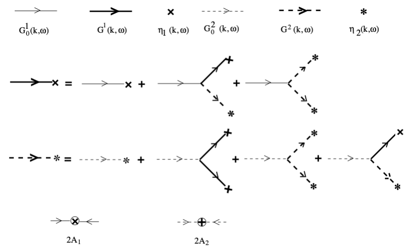
Figure 1: Symbols that are used for DRG calculation. Solid lines correspond to $h_{1}$ field and dashed lines correspond to $h_{2}$ field.

In the comoving frame of $h_{1}$, the dynamical equations (16) and (17) take the form

$$\partial_{t}h_{1}+b_{1}(\partial_{x}h_{1})(\partial_{x}h_{2})+c_{1}(\partial_{x}h_{2})^{2}=D_{1}\partial_{x}^{2}h_{1}+B_{1}\eta_{1}\,$$ (22)

$$\partial_{t}h_{2}+v\partial_{x}h_{2}+a_{2}(\partial_{x}h_{1})^{2}+b_{2}(\partial_{x}h_{1})(\partial_{x}h_{2})\\ +c_{2}(\partial_{x}h_{2})^{2}=D_{2}\partial_{x}^{2}h_{2}+B_{2}\eta_{2}\,$$ (23)

where the relative wave speed $v=v_{2}-v_{1}$ . The noises $\eta_{1}$ and $\eta_{2}$ are assumed to be zero-mean Gaussian distributed with variances

$$\langle\eta_{1}(x,t)\eta_{1}(x^{\prime},t^{\prime})\rangle = 2A_{1}\delta(x-x^{\prime})\delta(t-t^{\prime}),$$ (24)

$$\langle\eta_{2}(x,t)\eta_{2}(x^{\prime},t^{\prime})\rangle = 2A_{2}\delta(x-x^{\prime})\delta(t-t^{\prime})\,.$$ (25)

We need to solve Eqs. (22-23) perturbatively and obtain the fluctuation corrections to the model parameters. Symbols that are used in DRG calculations are shown in Fig. 1 .

From the linear part of the equations (22-23) we calculate $G_{0}^{1}(k,\omega)$ and $G_{0}^{2}(k,\omega)$ , the bare propagators of $h_{1}(k,\omega)$ and $h_{2}(k,\omega)$ respectively. Bare propagators are

$$G_{0}^{1}(k,\omega)=\frac{1}{D_{1}k^{2}+i\omega},$$ (26)

$$G_{0}^{2}(k,\omega)=\frac{1}{D_{2}k^{2}+i(\omega-kv)}.$$ (27)

Now notice that Eq. (22) for the dynamics of $h_{1}$ does not contain the KPZ-like nonlinear term $(\partial_{x}h_{1})^{2}$, although it is not prohibited by any symmetry arguments. In contrast, Eq. (23) contains all possible symmetry permitted bilinear nonlinearities of $\partial_{x}h_{1}$ and $\partial_{x}h_{2}$. Unsurprisingly, in an iterative, bare perturbation theory such KPZ-like nonlinear terms are indeed generated in Eq. (22). These terms are represented graphically in Fig. 2 . Let $a_{1}$ be the effective coefficient of the term $(\partial_{x}h_{1})^{2}$ that is generated in iterative expansions. We are thus obliged to add this term to Eq. (22) for consistency reasons before applications of DRG:

$$\partial_{t}h_{1}+a_{1}(\partial_{x}h_{1})^{2}+b_{1}(\partial_{x}h_{1})(\partial_{x}h_{2})\\ +c_{1}(\partial_{x}h_{2})^{2}=D_{1}\partial_{x}^{2}h_{1}+B_{1}\eta_{1}\,$$ (28)

The form of $a_{1}$ as obtained in the lowest order iterative expansion is given in Appendix.

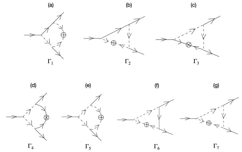
Figure 2: Generation of KPZ-like nonlinear terms with coefficient $a_{1}$ in the iterative expansions. Terms (a)-(c) originate from the vertex $b_{1}$, terms (d)-(g) are generated from the vertex $c_{1}$ .

That a term of the form $(\partial_{x}h_{1})^{2}$ is generated under iterative expansion is not surprising. Equations (22) and (28) have the same symmetries; in other words the absence of $(\partial_{x}h_{1})^{2}$ in (22) is not symmetry-protected, i.e., there is no symmetry that forbids the existence of this term in (22). Since Eqs. (28) and (23) and Eqs. (22) and (23) have exactly the same symmetries, they must belong to the same universality class. Furthermore, from the explicit forms of the one-loop expressions as given in Appendix, it is clear that these are inhomogeneous, which means $a_{1}=0$ is not a fixed point at all of this model. This remains an important technical conclusion from the present study.

The presence of the term $(\partial_{x}h_{1})^{2}$ in Eq. (28) can be further motivated phenomenologically as follows. Consider Eq. (16). Since the hydrodynamic equations are actually written down by expanding around uniform steady states assuming small fluctuations, the phenomenological coefficient $v_{1}$, assumed constant here, can actually depend upon the local fields in ways that respect the overall symmetries of the dynamics, i.e., invariance under constant shifts of $h_{1}$ and $h_{2}$. This consideration allows us to generalize $v_{1}$ and replace it by a field-dependent coefficient $v_{1}^{\prime}\equiv v_{1}+\tilde{a}_{1}\partial_{x}h_{1}$, where $\tilde{a}_{1}$ is a phenomenological constant coefficient. We now use this in Eq. (16); the resulting equation has the same form as Eq. (28). Here, two short technical comments are in order: (i) The coefficient $v_{1}^{\prime}$ can depend not only on $\partial_{x}h_{1}$, but also on $\partial_{x}h_{2}$ and all other terms that involve more fields and/or more derivatives. Inclusion of these terms do not generate any new relevant (in a DRG sense) terms in the resulting final equation. (ii) Secondly, all the other coefficients in Eqs. (16) and (17) too can depend on the local fields, subject to the overall symmetries. Again, inclusion of these contributions do not affect the physics in the long wavelength limit. We, therefore, ignore all these irrelevant contributions.

We work with the following effective equations, which are the most general equations with all possible symmetry-permitted nonlinear terms, written in the comoving frame of $h_{1}$:

$$\partial_{t}h_{1}+a_{1}(\partial_{x}h_{1})^{2}+b_{1}(\partial_{x}h_{1})(\partial_{x}h_{2})\\ +c_{1}(\partial_{x}h_{2})^{2}=D_{1}\partial_{x}^{2}h_{1}+\eta_{1},$$ (29)

$$\partial_{t}h_{2}+v\partial_{x}h_{2}+a_{2}(\partial_{x}h_{1})^{2}+b_{2}(\partial_{x}h_{1})(\partial_{x}h_{2})\\ +c_{2}(\partial_{x}h_{2})^{2}=D_{2}\partial_{x}^{2}h_{2}+\eta_{2},$$ (30)

where the factors of $B_{1}$ and $B_{2}$ have been absorbed in $\eta_{1}$ and $\eta_{2}$, respectively, for convenience, and $v\equiv v_{2}-v_{1}$. Since a term $(\partial_{x}h_{1})^{2}$ is symmetry-permitted and is generated under iterative expansion, and has the same scaling dimension as the existing nonlinear terms ep_pre , any RG analysis must start with an equation that already includes this term, even though the naive hydrodynamic theory may not have it. Thus Eqs. (29) and (30) should be the starting equations for any dynamic RG analysis for this problem. Equations (29) and (30) are identical to those studied in Ref. ep_pre by means of DRG and Monte-Carlo simulations. We do not repeat the calculation which is straightforward and instead refer the reader to Ref. ep_pre for the details, and revisit the conclusions of Ref. ep_pre below. It has been shown in Ref. ep_pre that the model belongs to the 1D KPZ universality class where $\chi_{1}=\chi_{2}=1/2$, together with a single dynamic exponent $z=3/2$. These led us to conclude that case C in the present study belongs to the 1D KPZ universality as well.

Our scheme of calculations follow the scheme outlined in Refs. mustansir ; ep_pre . Under perturbative DRG, no new relevant terms are further generated. We obtain the fluctuation corrections up to the one-loop order. As in Ref. ep_pre , each model parameter receives corrections that either originate from only the KPZ-like nonlinearities result (equivalently, from one-loop diagrams that are identical to those in the DRG for the KPZ equation), or nonlinearities other than the KPZ-type. For reasons identical to those elaborated in Ref. ep_pre , the former class of the diagrams are more relevant than the other diagrams in the long wavelength limit. As in Ref. ep_pre coupling constants do not receive any fluctuation corrections at the one-loop order in the long wavelength limit. We retain only these most dominant corrections. Rescaling space, time and fields as mentioned above the different RG flow equations read

$$\frac{dD_{1}}{dl} = D_{1}[z-2+g]\,,$$

$$\frac{dA_{1}}{dl} = A_{1}[z-1-2\chi_{1}+g]\,,$$

$$\frac{dD_{2}}{dl} = D_{2}[z-2+\frac{1}{2}mnrg]\,,$$

$$\frac{dA_{2}}{dl} = A_{2}[z-1-2\chi_{2}+pn^{2}g]\,,$$ (31)

where the coupling constant $g=\frac{A_{1}a_{1}^{2}}{\pi D_{1}^{3}}$ and dimensionless constants $m=\frac{D_{1}}{D_{2}}$, $p=\frac{A_{1}}{A_{2}}$, $n=\frac{a_{2}}{a_{1}}$, and $r=\frac{b_{1}}{a_{1}}$ . Unsurprisingly, these are identical to those derived in Ref. ep_pre . We therefore conclude $z=3/2,\,\chi_{1}=\chi_{2}=1/2$. Thus, the model belongs to the KPZ universality class.

It remains to be seen how one may arrive at the same conclusion from a OLSC study of case C. In an OLSC treatment, one is required to solve all the correlation and response functions, and also the nonlinear vertices self-consistently that received corrections that are unbounded or diverge in the thermodynamic limit at the one-loop order relative to their bare values in the theory amit-ab-jkb . OLSC further necessitates that at the one-loop order no new term should appear that would change the OLSC scaling if it were already present in the original theory. This consideration yields $z=3/2$ and $\chi=1/2$ for the 1D KPZ equation mustansir . Applying this to case C here, we note that Eq. (22) does not contain any $(\partial_{x}h_{1})^{2}$ term, i.e., the “bare” value of $a_{1}$ is zero. On the other hand, as stated above, a term of the form $(\partial_{x}h_{1})^{2}$ with a finite coupling coefficient $a_{1}$ is generated at the one-loop order. This conclusion remains unchanged even when one uses the self-consistent scaling forms for the correlation functions and the propagators. Since the “bare” value of $a_{1}$ is zero, self-consistent generation of a finite $a_{1}$ at the one-loop order implies a generation of a one-loop correction that, relative to its bare value, is infinitely large, and hence cannot be dropped. In other words, not retaining this correction would result a non self-consistent solution. Since the presence of a “bare” term of the form $(\partial_{x}h_{1})^{2}$ can affect the scaling exponents, we are required to include it before embarking on OLSC calculations. Once included, the OLSC calculations should reproduce  ep_pre directly that give $z=3/2,\chi_{1}=\chi_{2}=1/2$, in agreement with the DRG analysis discussed above.

Finally, we make one technical comment. We have argued above that even if the “bare” value of $a_{1}$ is zero, it is generated due to fluctuation effects. However, in order for it to be effective or relevant, it must be large enough, i.e., ${\cal O}(1)$. The size of the fluctuation-induced $a_{1}$, as shown in Appendix, depends upon all the other parameters and also on the system size. We thus expect that to extract the true asymptotic long wavelength scaling behavior, the system size should be sufficiently large enough. Further numerical investigations should be helpful in this context.

VI Summary and outlook

In summary, we have revisited the universal scaling properties of the density fluctuations in two-species periodic asymmetric exclusion processes. We argue that the continuum hydrodynamic equations of motion that one naively writes down does not include all the symmetry-permitted nonlinear terms. In fact, simple perturbative expansions produce the missing nonlinearity that is as relevant as the existing nonlinear terms. Hence, we argue that it should be included before undertaking any dynamic RG analysis on this model. Once this nonlinearity is considered, the effective equations of motion become identical to those analyzed in Ref. ep_pre . This in fact immediately allows us to conclude that the universal scaling exponents are identical to those for the 1D KPZ equation. That we get 1D KPZ scaling, in spite of having two conservation laws (corresponding to two conserved species) should not be surprising. This happens because, the coupled equations that include the extra nonlinear term, added on symmetry grounds, decouple in the long wavelength limit into two independent 1D KPZ equations. We note in the passing that our conclusions are at variance with Ref. popkov , where OLSC method was employed to calculate the universal scaling exponents. They did not consider the missing symmetry-permitted nonlinear term while applying OLSC, and obtained different values of the scaling exponents. We believe, if the OLSC method is employed after inclusion of this missing nonlinear term, it should yield the same results as here, for reasons similar to Ref. mustansir . Our results can be confirmed by solving the stochastically driven hydrodynamic equations numerically.

The OLSC method used elsewhere intrinsically ignores the vertex corrections, and can work well where the vertex correction is absent due to some symmetry reasons, e.g., the KPZ equation. In the present problem, there are no symmetry reasons that prohibit fluctuation corrections to all the coupling constants. However, due to the presence of the underdamped waves, the vertex corrections turn out to be finite ep_pre , and hence can be ignored so far as the universal scaling is concerned. The DRG framework can handle the vertex corrections, whether relevant (in the RG sense), or not - systematically. The generic question to what degree the universal scaling is affected by a missing coupling constant can occur in a theory with relevant vertex corrections as well. In such cases, applications of DRG methods would in fact be unavoidable.

Our work can be extended in a variety of ways. It will be interesting to extend our analysis to multi component models; see, e.g., Ref. van . It will also be interesting to construct a suitable higher dimensional version of the two-species asymmetric exclusion and obtain the corresponding higher dimensional hydrodynamic equations. One can then ask whether the higher dimensional version of the present model belongs to the higher dimensional KPZ universality class. Secondly, one can introduce “reactions” of various kinds, that will reduce the number of conservation laws from two to one. How that affects the long wavelength universal scaling properties is an interesting question to study in the future. One may additionally introduce lane exchanges by the particles and see whether the conclusions drawn here still remain valid in the presence of exchange. Effects of quenched disorder on the universal scaling properties can also be studied. It has recently been shown that in a single-component periodic TASEP with quenched disordered hopping rates, the disorder is irrelevant (in a RG sense) when the system is away from half-filling, and the scaling properties of the fluctuations in the long wavelength limit belong to the 1D KPZ universality class. In contrast, close to half-filling a new universality class emerges astik-prr . We hope our work will inspire future theoretical work along these directions.

Acknowledgements: One of us (AB) thanks the SERB, DST (India) for partial financial support through the MATRICS scheme [file no.: MTR/2020/000406].

Appendix

Linear stability analysis: Contribution of the pure diffusive terms

We consider Equations (16-17) with cross-diffusive terms. These equations can be written as

$$\partial_{t}h_{1}+v_{1}\partial_{x}h_{1}+b_{1}(\partial_{x}h_{1})(\partial_{x}h_{2})\\ +c_{1}(\partial_{x}h_{2})^{2}=D_{11}\partial_{x}^{2}h_{1}+D_{12}\partial_{x}^{2}h_{2}+B_{1}\eta_{1},$$ (32)

$$\partial_{t}h_{2}+v_{2}\partial_{x}h_{2}+a_{2}(\partial_{x}h_{1})^{2}+b_{2}(\partial_{x}h_{1})(\partial_{x}h_{2})\\ +c_{2}(\partial_{x}h_{2})^{2}=D_{21}\partial_{x}^{2}h_{1}+D_{22}\partial_{x}^{2}h_{2}+B_{2}\eta_{2}\,.$$ (33)

Taking Fourier transform on both sides above equations can be written as

$$\left[\begin{array}[]{c}\partial_{t}\tilde{h}_{1}\\ \partial_{t}\tilde{h}_{2}\end{array}\right]=M^{-1}\left[\begin{array}[]{c}B_{1}\eta_{1}\\ B_{2}\eta_{2}\end{array}\right]$$

where $\tilde{h}_{1}$, $\tilde{h}_{2}$ are the Fourier transforms of $h_{1}$ and $h_{2}$ respectively and

$$M=\left[\begin{array}[]{cc}-ikv_{1}+D_{11}k^{2}&D_{12}k^{2}\\ D_{21}k^{2}&-ikv_{2}+D_{22}k^{2}\\ \end{array}\right]$$

Eigenvalues of matrix $M$ are

$$\lambda_{1,2}=\frac{1}{2}\left[-ik(v_{1}+v_{2})+(D_{11}+D_{22})k^{2}\right]\\ \pm\frac{1}{2}\sqrt{\alpha_{1}k^{2}+2i\alpha_{2}k^{3}+\alpha_{4}k^{4}}$$ (34)

$\alpha_{1}=-(v_{1}-v_{2})^{2}$, $\alpha_{2}=(v_{1}D_{22}+v_{2}D_{11}-v_{1}D_{11}-v_{2}D_{22})$ , $\alpha_{4}=(-4D_{12}D_{21}+(D_{11}-D_{22})^{2})$ . For small $k$ , terms containing $k^{4}$ and $k^{3}$ are negligible compared to that with $k$. For small $k$, eigenvalues will be

$$\lambda_{1}=\frac{1}{2}\left[-2ikv_{2}+(D_{11}+D_{22})k^{2}\right]$$ (35)

$$\lambda_{2}=\frac{1}{2}\left[-2ikv_{1}+(D_{11}+D_{22})k^{2}\right]$$ (36)

This confirms that the pure diffusive terms have more dominant contributions than the cross diffusive terms to the eigenvalues.

Generation of the KPZ-like nonlinear term with coefficient $a_{1}$, that are generated in the one loop expansion

We give below the value of the coefficient $a_{1}$ obtained in the one loop expansions (see Fig. 2).

$$a_{1}=\Gamma_{1}+\Gamma_{2}+\Gamma_{3}+\Gamma_{4}+\Gamma_{5}+\Gamma_{6}+\Gamma_{7},$$ (37)

where

$$\Gamma_{1}=\frac{2A_{2}b_{1}b_{2}}{\pi D_{2}^{2}} \int\frac{(4q^{2}-k_{1}^{2})dq}{\left[k_{1}^{2}+4k_{2}^{2}-4k_{1}q-8k_{2}q+8q^{2}\right]}$$

$$\times\frac{1}{\left[4D_{2}(k_{2}-q)^{2}-2iv(k_{1}+2q)+D_{1}(k_{1}+2q)^{2}\right]}$$

$$\times\frac{\left[-2iv(k_{1}+2q)+D_{1}(k_{1}+2q)^{2}+D_{2}(k_{1}^{2}+8k_{2}^{2}-4k_{1}q-16k_{2}q+12q^{2})\right]}{\left[D_{2}(k_{1}-2q)^{2}+D_{1}(k_{1}+2q)^{2}-2iv(k_{1}+2q)\right]}$$

$$\Gamma_{2}= -\frac{4A_{2}b_{1}b_{2}}{\pi D_{2}^{2}}\int\frac{(k_{2}+q)(k_{1}+2q)dq}{\left[k_{1}^{2}+4k_{2}^{2}-4k_{1}q+8q(k_{2}+q)\right]}$$ (39)

$$\times\frac{1}{\left[D_{2}(k_{1}-2q)^{2}-2iv(k_{1}+2q)+D_{1}(k_{1}+2q)^{2}\right]}$$ (40)

$$\Gamma_{3}= \frac{16A_{1}a_{2}b_{2}}{\pi}\int\frac{(k_{1}-2q)^{2}(k_{2}+q)(k_{1}+2q)}{\left[2v(k_{1}-2q)-i(D_{1}(k_{1}-2q)^{2}-4D_{2}(k_{2}+q)^{2})\right]}$$

$$\times\frac{\left[-4iv(k_{1}-2q)+D_{2}(k_{1}^{2}+4k_{2}^{2}+4k_{1}q+8q(k_{2}+q)\right]}{\left[2v(k_{1}-2q)+i(D_{1}(k_{1}-2q)^{2}+4D_{2}(k_{2}+q)^{2})\right]}$$

$$\times\frac{1}{\left[2v(k_{1}-2q)-i\left[D_{1}(k_{1}-2q)^{2}-D_{2}(k_{1}+2q)^{2}\right]\right]}$$

$$\times\frac{1}{\left[2v(k_{1}-2q)+i\left[D_{1}(k_{1}-2q)^{2}+D_{2}(k_{1}+2q)^{2}\right]\right]}$$

$$\Gamma_{4}= \frac{32A_{1}a_{2}^{2}}{\pi}\int\frac{(k_{1}^{2}-4q^{2})(q-k_{2})^{2}dq}{D_{2}(k_{1}^{2}+4q^{2})\left[4(-iv+D_{1}(k_{2}-q))(k_{2}-q)+D_{2}(k_{1}+2q)^{2}\right]}$$

$$\times\frac{1}{\left[-4(iv+D_{1}(k_{2}-q))(k_{2}-q)+D_{2}(k_{1}+2q)^{2}\right]}$$

$$\Gamma_{5}= \frac{2A_{2}b_{2}^{2}}{\pi}\int\frac{(4q^{2}-k_{1}^{2})dq}{D_{2}^{3}(k_{1}^{2}+4q^{2})\left[k_{1}^{2}+4k_{2}^{2}-4(k_{1}+2k_{2})q+8q^{2}\right]}$$

$$\times\frac{(k_{1}^{2}+4k_{2}^{2}-8k_{2}q+8q^{2})}{\left[k_{1}^{2}+4k_{2}^{2}+4(k_{1}-2k_{2})q+8q^{2}\right]}$$

$$\Gamma_{6}=-\frac{8A_{2}a_{2}b_{1}}{\pi}\int\frac{(k_{2}+q)(k_{1}+2q)dq}{D_{2}^{2}(k_{1}^{2}+4q^{2})\left[D_{2}(k_{1}-2q)^{2}+4(k_{2}+q)(-iv+D_{1}(k_{2}+q))\right]}$$ (44)

$$\Gamma_{7}=-\frac{4A_{2}b_{2}^{2}}{\pi}\int\frac{(k_{2}+q)(k_{1}+2q)dq}{D_{2}^{3}(k_{1}^{2}+4q^{2})\left[k_{1}^{2}+4k_{2}^{2}-4k_{1}q+8q(k_{2}+q)\right]}$$ (45)

References

- (1) Statistical mechanics of driven diffusive systems, B. Schmittmann, R.K.P. Zia, Phase Transitions and Critical Phenomena, Academic Press, Volume 17, 1995.
- (2) M. Kardar, G. Parisi and Yi-Cheng Zhang, Phys. Rev. Lett. 56, 889 (1986).
- (3) A. Basu, J.K. Bhattacharjee and S. Ramaswamy, Euro. Phys. J. B, 9, 725 (1999).
- (4) D. Das, A. Basu, M. Barma and S. Ramaswamy, Phys. Rev. E, 64, 021402 (2001).
- (5) P. Dolai, Abhik Basu and Aditi Simha, Phys. Rev. E, 95, 052115 (2017).
- (6) P. L. Ferrari, T. Sasamoto and H. Spohn, J. Stat. Phys. 153, 377 (2013).
- (7) C. Arita, A. Kuniba, K. Sakai and T. Sawabe, J. Phys. A, 42, 345002 (2009).
- (8) A. Rákos and G. M. Schütz, J. Stat. Phys. 117, 55 (2004).
- (9) Principles of condensed matter physics, P. M. Chaikin and T. C. Lubensky, Cambridge University Press, 1995.
- (10) V. Popkov, J. Schmidt and G. M. Schütz, Phys. Rev. Lett. 112, 200602 (2014).
- (11) H. Spohn and G. Stoltz, J. Stat. Phys. 160, 861 (2015).
- (12) H. Spohn, J. Stat. Phys. 154, 1191 (2014).
- (13) Proceedings of the Les Houches Summer School of Theoretical Physics, H. Spohn, Oxford University Press, 2016.
- (14) J. Schmidt and G. M. Schütz and H. van Beijeren, J. Stat. Phys. 183, 8 (2021).
- (15) V. Popkov and G. M. Schütz, J. Stat. Phys. 112, 523 (2003).
- (16) D. Forster, D. R. Nelson and M. J. Stephen, Phys. Rev. A, 16, 732 (1977).
- (17) Fractal concepts in surface growth, A. L. Barabasi and H. E. Stanley, Cambridge University Press, 1995.
- (18) L. H. Tang, T. Nattermann and B. M. Forrest, Phys. Rev. Lett, 65, 2422 (1990).
- (19) Hydrodynamic Fluctuations, Broken Symmetry, and Correlation Functions, D. Foster, CRC Press 1995.
- (20) C. De Dominicis, J. Phys. (Paris) Colloq. C, 1, 247 (1976).
- (21) H.K. Janssen, Z. Phys. B, 23, 377 (1976).
- (22) P. C. Hohenberg and B. I. Halperin, Rev. Mod. Phys. 49, 435 (1977).
- (23) T. Halpin-Healy and Yi-Cheng Zhang, Phys. Rep. 254, 215 (1995).
- (24) A. K. Chattopadhyay, A. Basu and J. K. Bhattacharjee, Phys. Rev. E, 61, 2086 (2000).
- (25) A. Haldar and A. Basu, Phys. Rev. Res. 2, 043073 (2020).